A spectroscopic model for the low-lying electronic states of NO

Abstract

The rovibronic structure of $\mathrm{A}\,{}^{2}\Sigma^{+}$, $\mathrm{B}\,{}^{2}\Pi$ and $\mathrm{C}\,{}^{2}\Pi$  states of nitric oxide (NO) is studied with the aim of producing comprehensive line lists for its near ultraviolet spectrum. Empirical energy levels for the three electronic states are determined using the a combination of the empirical MARVEL procedure and ab initio calculations, and the available experimental data are critically evaluated. Ab inito methods which deal simultaneously with the Rydberg-like $\mathrm{A}\,{}^{2}\Sigma^{+}$ and $\mathrm{C}\,{}^{2}\Pi$, and the valence $\mathrm{B}\,{}^{2}\Pi$ state are tested. Methods of modeling the sharp avoided crossing between the $\mathrm{B}\,{}^{2}\Pi$ and $\mathrm{C}\,{}^{2}\Pi$ states are tested. A rovibronic Hamiltonian matrix is constructed using variational nuclear motion program Duo whose eigenvalues are fitted to the MARVEL energy levels. The matrix also includes coupling terms obtained from the refinement of the ab initio  potential energy and spin-orbit coupling curves. Calculated and observed energy levels agree well with each other, validating the applicability of our method and providing a useful model for this open shell system.

I Introduction

Nitric oxide (NO) is one of the principle oxides of nitrogen. It plays a significant role in the nitrogen cycle of our atmosphere Canfield, Glazer, and Falkowski (2010); Vitousek et al. (1997) but also causes problems of air pollution and acid rain Chameides et al. (1994); Likens, Driscoll, and Buso (1996); Singh and Agrawal (2007). Therefore, scientists are devoting increasing attention to reducing NO in combustion processes Hu et al. (2000); Li, Lu, and Rudolph (1998). NO is a biological messenger for both animals and plants Bredt and Snyder (1992, 1994); Arasimowicz and Floryszak-Wieczorek (2007) but it may be harmful or even deadly as well Mayer and Hemmens (1997); Estévez and Jordán (2002). Apart from on Earth, NO was also observed in the interstellar environments and atmospheres of other planets Ziurys et al. (1991); Cox et al. (2008); Gérard et al. (2008, 2009).

The importance of NO has aroused the interest of academia and industry since it was prepared by van Helmont in the 17th century Partington (1936) and then studied by Priestley in 1772 Priestley (1772). In numerous theoretical and experimental works, there are large number of spectroscopic investigations, as spectra provide a powerful weapon to reveal the physical and chemical properties of the molecule. For instance, as a stable open shell molecule, the electronically excited Rydberg states of NO have been extensively studies, see the paper of Deller and HoganDeller and Hogan (2020) and references therein. The spectrum of NO was also of great value in many applications, such as temperature measurements by laser induced fluorescenceBessler and Schulz (2004); Van Gessel et al. (2013).

The ExoMol projectTennyson and Yurchenko (2012) computes molecular line lists studies of exoplanet and (other) hot atmospheres. The ExoMol database was formally released in 2016 Tennyson et al. (2016a). The most recent 2020 version Tennyson et al. (2020) covers the line lists of 80 molecules and 190 isotopologues, totaling 700 billion transitions. It includes an accurate infrared (IR) line list of NO, called NOname, which contains the rovibrational transitions within the ground electronic state Wong et al. (2017). The rovibronic transitions of NO in the ultraviolet (UV) region are not included in NOname. These bands are strong, atmospherically important and have been observed in many studies Lagerqvist and Miescher (1958); Danielak et al. (1997); Yoshino et al. (2006). There is no NO UV line list in well-known databases such as HITRAN Gordon et al. (2017) and GEISA Jacquinet-Husson et al. (2016) either.

Luque and Crosley have investigated spectra of diatomic molecules over a long period Luque and Crosley (1995, 1999a, 2000). Based on their works, they developed a spectral simulation program, LIFBASE Luque and Crosley (1999b), providing a database of OH, OD, CH etc., and NO as well. LIFBASE contains the positions and relative probabilities of UV transitions in four spectral systems of NO, i.e., $\upgamma$ ($\mathrm{A}\,{}^{2}\Sigma^{+}$ to $\mathrm{X}\,{}^{2}\Pi$), $\upbeta$ ($\mathrm{B}\,{}^{2}\Pi$ to $\mathrm{X}\,{}^{2}\Pi$), $\updelta$ ($\mathrm{C}\,{}^{2}\Pi$ to $\mathrm{X}\,{}^{2}\Pi$) and $\upvarepsilon$ ($\mathrm{D}\,{}^{2}\Sigma^{+}$ to $\mathrm{X}\,{}^{2}\Pi$) systems. The upper vibrational energy levels for $\mathrm{B}\,{}^{2}\Pi$ and $\mathrm{C}\,{}^{2}\Pi$ of NO in LIFBASE are limited to below $v=7$ and $v=1$, respectively. However, the observed $\upbeta$ and $\updelta$ transitions corresponding to higher upper vibrational energy levels are even stronger Yoshino et al. (1998, 2006). There is a need to develop a comprehensive UV line list for NO to cover these band systems. To do this one first needs to construct a spectroscopic model which requires overcoming a number of theoretical difficulties. The purpose of this paper is to present our model and explain how we resolve these difficulties.

A major issue in generating a UV line list for NO results from the difficulty of modelling the interaction between $\mathrm{B}\,{}^{2}\Pi$ and $\mathrm{C}\,{}^{2}\Pi$ states, which is caused by the particular electronic structure of NO. To understand this fifteen electrons system one must analyse the electron configuration of these states from the perspective of molecular orbitals. On one hand, excitation of inner paired electrons to higher valence orbitals leads to valence states such as $\mathrm{B}\,{}^{2}\Pi$. On the other hand, the outermost unpaired electron may be excited to Rydberg orbitals, yielding a series of Rydberg states such $\mathrm{A}\,{}^{2}\Sigma^{+}$ or $\mathrm{C}\,{}^{2}\Pi$. These Rydberg states lie close in energy to the valence ones. Furthermore, as NO+ has a shorter equilibrium bondlength than NO Albritton, Schmeltekopf, and Zare (1979), Rydberg states tend to be lower in energy at short bondlengths, $r$, while valence states are lower at larger $r$. Thus, in NO, Rydberg-valence interactions are densely distributed in the neighbourhood of the equilibrium bond length of its ground state, where large Franck-Condon factors exist. The $\mathrm{B}\,{}^{2}\Pi$  - $\mathrm{C}\,{}^{2}\Pi$ interaction is the lowest one and has attracted the most attention. As described by Lagerqivst and Miescher Lagerqvist and Miescher (1958), the two states show a strong and extended mutual perturbation. They proposed a ‘deperturbation’ method to explain the vibrational and rotational perturbation of $\mathrm{B}\,{}^{2}\Pi$  - $\mathrm{C}\,{}^{2}\Pi$ interaction. Further analysis was made by Gallusser and Dressler Gallusser and Dressler (1982), who set up a vibronic interaction matrix of five ${}^{2}\Pi$ states and fitted the eigenvalues of the matrix to experimental data in the determination of RKR potential curves and off-diagonal electronic energies. As a consequence, they predicted vibrational states of the $\mathrm{B}\,{}^{2}\Pi$ electronic state up to $v=37$.

In this paper, we propose a method based on directly diagonalizing a rovibronic matrix to resolve the energy structures of $\mathrm{B}\,{}^{2}\Pi$  - $\mathrm{C}\,{}^{2}\Pi$ coupled states. This matrix is based on the use of full variational solution of the rovibronic nuclear motion Hamiltonian rather than perturbation theory. This method is general and can be used to predict spectra, for example at elevated temperatures.

In addition to the vibronic matrix elements (e.g., spin doublets) considered in the previous studies, more fine structure terms, such as $\varLambda$ - doubling and spin-rotational coupling, are used to construct the rovibronic matrix. The eigenvalues of the matrix are fitted to rovibronic energies obtained using a MARVEL (measured active rotation-vibration energy levels) procedure Furtenbacher, Császár, and Tennyson (2007a); Tóbiás et al. (2019) analysis of the observed NO IR/visible/UV transitions to ensure a quantitatively accurate result. Figure 1 summarizes the band systems involved in our MARVEL analysis. The objective functions were constrained with the ab initio curves produced using Molpro Werner et al. (2015) to avoid overfitting problems. The above procedures are also applied to the $\mathrm{A}\,{}^{2}\Sigma^{+}$ state of NO to get a self-consistent description of the doublet electronic states up to and including $\mathrm{C}\,{}^{2}\Pi$.

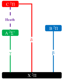
Figure 1: The band systems of NO involved in this work and their names. The $\upgamma$, $\upbeta$ and $\updelta$ systems mainly cover the UV transitions of NO. Jenkins et al. recorded many visible lines from $\mathrm{B}\,{}^{2}\Pi$ state to higher vibrational levels of $\mathrm{X}\,{}^{2}\Pi$, e.g., those of $\upbeta(3,16)$ band Jenkins, Barton, and Mulliken (1927). The high-accuracy IR transitions of $\mathrm{Heath}(0,0)$ band were measured by Amiot and Verges Amiot (1982). For a comprehensive band system diagram, see the work of Cartwright et al. Cartwright et al. (2000)

This work forms the foundation of our future study on the generation of UV line list of NO. The modeling of $\mathrm{B}\,{}^{2}\Pi$  - $\mathrm{C}\,{}^{2}\Pi$ paves the way for the investigations of molecules with similar avoided crossing structures.

II Theoretical study of the low-lying electronic states of NO

Complete active space self-consistent field (CASSCF) and multireference configuration interaction (MRCI) calculations were performed in the quantum chemistry package Molpro 2015 Werner et al. (2012) to get the potential energy and spin-orbit curves of the $\mathrm{X}\,{}^{2}\Pi$, $\mathrm{A}\,{}^{2}\Sigma^{+}$, $\mathrm{B}\,{}^{2}\Pi$ and $\mathrm{C}\,{}^{2}\Pi$ states. A major issue in the calculation is achieving a balance between representations of the Rydberg, A and C, states and the valence, X and B, states. Figure 2 presents an overview of the low-lying PECs and illustrates the importance of the $\mathrm{C}\,{}^{2}\Pi$– $\mathrm{B}\,{}^{2}\Pi$ Rydberg – Valence avoided crossing.

The history of high quality CI calculation for the excited states of NO can be tracked back to 1982, when Grein and Kapur reported their work on the states with the minimum electronic energies lower than $6.58\text{\,}\mathrm{eV}$ Grein and Kapur (1982). Several years later, a comprehensive theoretical study on NO were presented and discussed by de Vivie and Peyerimhoff Devivie and Peyerimhoff (1988). The results of this paper was further improved by Shi and East in 2006 Shi and East (2006). More accurate curves were obtained with extended basis set and active space in the recent works of Cheng et al. Cheng, Zhang, and Cheng (2017); Cheng et al. (2017). Although the previous works Grein and Kapur (1982); Cooper (1982); Langhoff, Bauschlicher, and Partridge (1988); Devivie and Peyerimhoff (1988); Langhoff et al. (1991); Polak and Fiser (2003); Shi and East (2006); Cheng, Zhang, and Cheng (2017) provide us strong inspiration, the task is still challenging due to the interactions between Rydberg and valence states of NO.

II.1 Active space and basis set

For heteronuclear diatomic molecules, Molpro executes calculations in four irreducible representations $a_{1}$, $b_{1}$, $b_{2}$ and $a_{2}$ of the $C_{\mathrm{2v}}$ point group. Here, we use $[(n_{1},n_{2},n_{3},n_{4})-(n^{\prime}_{1},n^{\prime}_{2},n^{\prime}_{3},n^{\prime}_{4})]$ to represent occupied orbitals excluding closed orbitals, i.e. the calculation active space. A typical active space for the lower electronic states calculation of NO is $[(8,3,3,0)-(2,0,0,0)]$, as suggested by Shi and East Shi and East (2006). Although only a few of the PECs are of direct interest here, we had to include extra states to achieve correct calculation. We also adjusted the active space to get smooth curves.

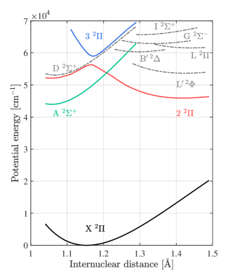
Figure 2: NO PECs calculated by Shi and East Shi and East (2006). The states of interest are plotted by solid curves. Here, $2\,^{2}\Pi$ is the $\mathrm{B}\,{}^{2}\Pi$ to $\mathrm{C}\,{}^{2}\Pi$ PEC while $3\,^{2}\Pi$ is the $\mathrm{C}\,{}^{2}\Pi$ to $\mathrm{B}\,{}^{2}\Pi$ PEC.

A Dunning aug-cc-pV(n)Z basis set Dunning (1989) was used in both CASSCF and MRCI calculation. This basis set has an additional shell of diffuse functions compare to the cc-pV(n)Z basis set, which benefits the calculation of Rydberg states. Too many diffuse functions, e.g., those of the d-aug-cc-pV(n)Z basis set, may have negative effects on the calculation because of the overemphasis of the Rydberg states relative to the valence states.

II.2 CASSCF calculation

Our calculations started with a $[(8,3,3,0)-(2,0,0,0)]$ active space in which the interactions between the Rydberg and valence states are inescapable. However, representing the avoided crossing points caused by $\mathrm{C}\,{}^{2}\Pi$ and the valence ${}^{2}\Pi$ states proved to be a huge obstacle to obtaining satisfactory results. Panel (a) of Fig. 3 shows the terrible behavior of B - C interaction near $1.18\text{\,}\mathrm{\SIUnitSymbolAngstrom}$. The potential energy curve (PEC) of $\mathrm{C}\,{}^{2}\Pi$ suddenly jumps to that of $\mathrm{B}\,{}^{2}\Pi$, producing discontinuity in the PEC of $\mathrm{X}\,{}^{2}\Pi$ too. To get the exited states, we used the state average algorithm but the average energy of the two ${}^{2}\Pi$ states changed when traversing the crossing point of $\mathrm{C}\,{}^{2}\Pi$ and $\mathrm{B}\,{}^{2}\Pi$.

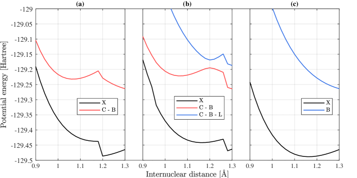
Figure 3: The PECs in the active space of $[(8,3,3,0)-(2,0,0,0)]$ with the basis set of aug-cc-pVTZ. (a) Two ${}^{2}\Pi$ states averaged CASSCF calculation starting from $0.9\text{\,}\mathrm{\SIUnitSymbolAngstrom}$. (b) Three ${}^{2}\Pi$ states averaged CASSCF calculation starting from $0.9\text{\,}\mathrm{\SIUnitSymbolAngstrom}$. (c) Two ${}^{2}\Pi$ states averaged CASSCF calculation starting from $1.3\text{\,}\mathrm{\SIUnitSymbolAngstrom}$.

A valid way to smooth the curves is to increase the number of averaged states. For example, the discontinuities near $1.18\text{\,}\mathrm{\SIUnitSymbolAngstrom}$ disappears when introducing a third ${}^{2}\Pi$ state in CASSCF calculation, as shown in Panel (b) of Fig. 3. Nevertheless, similar phenomenon arises when the third state comes across $\mathrm{L}\,{}^{2}\Pi$. Alternatively, smooth curves can be obtained in limited active space. For example, we can get a continuous curves of $\mathrm{C}\,{}^{2}\Pi$ in the active space $[(6,3,3,0)-(4,1,1,0)]$ from $0.9\text{\,}\mathrm{\SIUnitSymbolAngstrom}$ to $1.28\text{\,}\mathrm{\SIUnitSymbolAngstrom}$.

We always started a new CASSCF iteration from the orbitals of a nearby geometry to stabilize and accelerate the calculation. The PECs in Panels (a) and (b) of Fig. 3, are obtained by increasing the internuclear distance from $0.9\text{\,}\mathrm{\SIUnitSymbolAngstrom}$ to $1.3\text{\,}\mathrm{\SIUnitSymbolAngstrom}$. Interestingly, with a initial geometry at $1.3\text{\,}\mathrm{\SIUnitSymbolAngstrom}$, reversing the calculation direction gives a completely different result in the same active space, i.e., two smooth valence PECs of $\mathrm{X}\,{}^{2}\Pi$ and $\mathrm{B}\,{}^{2}\Pi$ states in Panel (c) of Fig. 3. Due to the limitation of nonlinear programming, CASSCF iterations may fall into local minima. To get the target states, the numerical optimization must be properly initialized. For the NO molecule, the iterations which begin with valence orbitals usually end with valence orbitals but it is uncertain for those begin with Rydberg orbitals. The results imply that there are at least two kinds of local minimums in the ab initio calculation of NO with Molpro: pure valence orbitals (corresponding to Panel (c) of Fig. 3) and Rydberg-valence hybrid orbitals (corresponding to Panels (a) and (b) of Fig. 3). To verify the conjecture: initializing a calculation of two ${}^{2}\Pi$ states average with the CASSCF orbitals of the $\mathrm{X}\,{}^{2}\Pi$ state in the single state calculation, one can get almost the same curves as those in Panel (c) of Fig. 3, starting from $0.9\text{\,}\mathrm{\SIUnitSymbolAngstrom}$.

In Section IV, we use diabatic potentials in modeling interaction between $\mathrm{B}\,{}^{2}\Pi$ and $\mathrm{C}\,{}^{2}\Pi$ states. We describe the curves as ‘adiabatic’ if they contain the B - C avoided crossing feature, e.g., those in Panel (b) of Fig. 3. If not, we call the curves ‘diabatic’, e.g., those in Panel (c) of Fig. 3.

II.3 MRCI calculation

Although consuming many more computational resources, the MRCI calculation in Molpro is straightforward. Molpro automatically takes the CASSCF orbitals as the references and performs an internally contracted configuration interaction calculation based on single or double excitation. The spin-orbit coupling terms were also produced. To compensate the error brought by truncated configuration interaction expansion, the energies were modified by Davision correction, i.e., MRCI + Q calculation. Panel (a) of Fig. 4 demonstrates the results of CASSCF & MRCI + Q calculation of the $\mathrm{X}\,{}^{2}\Pi$, $\mathrm{A}\,{}^{2}\Sigma^{+}$, $\mathrm{B}\,{}^{2}\Pi$, $\mathrm{C}\,{}^{2}\Pi$, $\mathrm{D}\,{}^{2}\Sigma^{+}$ and $\mathrm{L}^{\prime}\,{}^{2}\Phi$ states, in $[(8,3,3,0)-(2,0,0,0)]$ active space with aug-cc-pV5Z basis set.

In the CASSCF routine, the projection of angular momentum of a diatomic molecule on its internuclear axis, $\varLambda$, can be assigned to specify the expected states. However, the MRCI routine does not have the option and always finds the lowest energy states of the same spin. As a result, the PECs of $\mathrm{C}\,{}^{2}\Pi$ and $\mathrm{L}^{\prime}\,{}^{2}\Phi$ exchange with each other at their crossing point although the avoided crossing principle is not applicable for the two states, as shown by the blue curve in Panel (a) of Fig. 4. It is feasible to calculate and output the $\varLambda$ quantum numbers (technically, Lz, which is defined as a non-diagonal matrix element between two degenerate components, e.g. $\matrixelement{\Pi_{x}}{\hat{L}_{z}}{\Pi_{y}}$) in MRCI calculations, which helps to distinguish the $\mathrm{C}\,{}^{2}\Pi$, $\mathrm{L}^{\prime}\,{}^{2}\Phi$ and $\mathrm{L}\,{}^{2}\Pi$ states. The blue and yellow curves on the right of their crossing point were manually switched, as shown in Panel (c) of Fig. 4, according to their $\varLambda$ quantum numbers shown in Panel (b). The $T_{e}$ values of $\mathrm{A}\,{}^{2}\Sigma^{+}$, $\mathrm{B}\,{}^{2}\Pi$ and $\mathrm{C}\,{}^{2}\Pi$ states are compared with those calculated by Shi and East in Table 1.

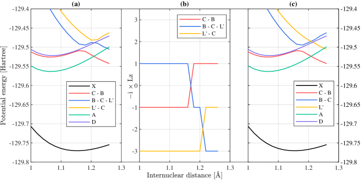
Figure 4: The PECs of the $\mathrm{X}\,{}^{2}\Pi$, $\mathrm{A}\,{}^{2}\Sigma^{+}$, $\mathrm{B}\,{}^{2}\Pi$, $\mathrm{C}\,{}^{2}\Pi$, $\mathrm{D}\,{}^{2}\Sigma^{+}$ and $\mathrm{L}^{\prime}\,{}^{2}\Phi$ states, obtained by CASSCF & MRCI + Q calculation starting from $1.06\text{\,}\mathrm{\SIUnitSymbolAngstrom}$ to both sides in the active space $[(8,3,3,0)-(2,0,0,0)]$ with the aug-cc-pV5Z basis set. The third ${}^{2}\Pi$ curve and the $\mathrm{L}^{\prime}\,{}^{2}\Phi$ curve in Panel (a) were manually switched in Panel (c) on the right of $1.2\text{\,}\mathrm{\SIUnitSymbolAngstrom}$, according to the value of Lz, shown in Panel (b). The phase of Lz, in the Cartesian representation, is random. To distinguish different electronic states, the yellow curve in Panel (b) is smoothed for internuclear distances less than $1.1\text{\,}\mathrm{\SIUnitSymbolAngstrom}$. The $\mathrm{X}\,{}^{2}\Pi$ state is not shown in the Panel as the Lz values obtained are all $-\mathrm{i}$.

Table 1: Comparison of $T_{e}$ values of the MRCI + Q calculation

State	CASSCF & MRCI + Q		Empirical
	Shi and East Shi and East (2006)	This work	Huber and Herzberg Huber and Herzberg (1979)	This work
$\mathrm{A}\,{}^{2}\Sigma^{+}$	$43\,558$	$45\,410.2$	$43\,965.7$	$43\,902.99$
$\mathrm{B}\,{}^{2}\Pi$	$44\,803$	$46\,260.3$	$45\,913.6$	$45\,867.05$
$\mathrm{C}\,{}^{2}\Pi$	$51\,808$	$53\,709.5$	$52\,126$	$52\,081.97$

The PECs in Fig. 4 range from $1.0\text{\,}\mathrm{\SIUnitSymbolAngstrom}1.26\text{\,}\mathrm{\SIUnitSymbolAngstrom}$. The curves were deliberately truncated at the right endpoint because of the $\mathrm{C}\,{}^{2}\Pi$  - $\mathrm{L}\,{}^{2}\Pi$ interaction as shown in Panel (b) of Fig. 3. On the left endpoint, The MRCI program exited with an ‘INSUFFICIENT OVERLAP’ error. The error is triggered by interactions with another ${}^{2}\Pi$ state, $\mathrm{H}^{\prime}\,{}^{2}\Pi$, which lies below $\mathrm{B}\,{}^{2}\Pi$ near the $1.06\text{\,}\mathrm{\SIUnitSymbolAngstrom}$ and which cannot be described by the reference space. A solution to the problem is to perform MRCI calculations using a larger active space such as $[(8,4,4,0)-(2,0,0,0)]$.

It is not quantitatively accurate to generate line lists with the ab initio curves; however, the curves and couplings provide a suitable starting point for work. These curves and couplings need to be refined using experimental data, which is the content of the subsequent two sections.

III MARVEL analysis of the rovibronic energy levels of ^14N^16O

The rovibronic energy levels of $\mathrm{A}\,{}^{2}\Sigma^{+}$, $\mathrm{B}\,{}^{2}\Pi$ and $\mathrm{C}\,{}^{2}\Pi$ states were reconstructed by MARVEL analysis of the experimental transitions of the $\upgamma$, $\upbeta$, $\updelta$, and $\mathrm{Heath}$ systems and those inside the ground state.

In the previous work by Wong et al. Wong et al. (2017), $11\,136$ IR transitions were collected, yielding a spectroscopic network of $4106$ energy levels. To retrieve the energy levels of $\mathrm{A}\,{}^{2}\Sigma^{+}$, $\mathrm{B}\,{}^{2}\Pi$ and $\mathrm{C}\,{}^{2}\Pi$ states, we extracted a further $9861$ transitions (including $3393$ $\upgamma$, $5103$ $\upbeta$, $1004$ $\updelta$ and $361$ Heath transitions) from the data sources listed in Table 2. The vibronic structure of the spectroscopic network is illustrated in Fig. 5.

Although there are studies which report measured transition frequencies for the four band systems of interest, only the most reliable data sets were included in our MARVEL analysis. For example, Lagerqvist and Miescher published the line position data of 20 bands of the $\upbeta$ and $\updelta$ systems ($\upbeta(5,0)$ to $\upbeta(19,0)$ and $\updelta(0,0)$ to $\updelta(4,0)$, respectively) in 1958 (58LaMi Lagerqvist and Miescher (1958)), but half of them were replaced by more accurate line lists measured by Yoshino et al. around 2000 (94MuYoEs Murray et al. (1994), 98YoEsPa Yoshino et al. (1998), 00ImYoEs Imajo et al. (2000), 02ChLoLe Cheung et al. (2002), 02RuYoTh Rufus et al. (2002), 06YoThMu Yoshino et al. (2006)).

Table 2: Data sources used in the final MARVEL analysis

Source	Band	$J_{\textrm{min}}^{\prime\prime}$	$J_{\textrm{max}}^{\prime\prime}$	Uncertainty	Trans.
				[$\mathrm{cm}^{-1}$]	(A)	(V)
97DaDoKe Danielak et al. (1997)	$\upgamma(0,0)$	0.5	41.5	0.04 - 0.15	304	277
97DaDoKe	$\upgamma(0,1)$	0.5	40.5	0.04 - 0.15	277	245
97DaDoKe	$\upgamma(0,2)$	1.5	39.5	0.04 - 0.15	339	317
97DaDoKe	$\upgamma(0,3)$	1.5	38.5	0.04 - 0.1	289	279
97DaDoKe	$\upgamma(0,4)$	1.5	42.5	0.04 - 0.1	294	283
97DaDoKe	$\upgamma(0,5)$	1.5	37.5	0.04 - 0.1	266	249
97DaDoKe	$\upgamma(0,6)$	1.5	31.5	0.04 - 0.15	158	142
97DaDoKe	$\upgamma(1,0)$	0.5	30.5	0.04 - 0.15	302	275
97DaDoKe	$\upgamma(1,4)$	0.5	41.5	0.04 - 0.15	295	277
97DaDoKe	$\upgamma(1,5)$	1.5	39.5	0.04 - 0.15	142	135
97DaDoKe	$\upgamma(2,6)$	1.5	40.5	0.04 - 0.15	277	246
97DaDoKe	$\upgamma(2,7)$	2.5	41.5	0.04 - 0.15	160	155
02ChLoLe Cheung et al. (2002)	$\upgamma(3,0)$	0.5	24.5	0.03 - 0.05	227	205
97DaDoKe	$\upgamma(3,4)$	4.5	32.5	0.04 - 0.2	63	56
27JeBaMu Jenkins, Barton, and Mulliken (1927)	$\upbeta(0,4)$	0.5	24.5	0.2	122	52
27JeBaMu	$\upbeta(0,5)$	0.5	24.5	0.2	152	143
27JeBaMu	$\upbeta(0,6)$	0.5	24.5	0.2	126	124
27JeBaMu	$\upbeta(0,7)$	0.5	29.5	0.2	202	200
27JeBaMu	$\upbeta(0,8)$	0.5	31.5	0.2	206	204
27JeBaMu	$\upbeta(0,9)$	0.5	31.5	0.2	192	188
27JeBaMu	$\upbeta(0,10)$	0.5	31.5	0.2	208	202
27JeBaMu	$\upbeta(0,11)$	0.5	31.5	0.2	184	180
27JeBaMu	$\upbeta(0,12)$	0.5	22.5	0.2	138	138
27JeBaMu	$\upbeta(1,6)$	0.5	19.5	0.2	123	119
27JeBaMu	$\upbeta(1,11)$	0.5	24.5	0.2	148	142
27JeBaMu	$\upbeta(1,13)$	0.5	23.5	0.2	154	150
27JeBaMu	$\upbeta(2,9)$	0.5	22.5	0.2	138	130
27JeBaMu	$\upbeta(2,13)$	0.5	21.5	0.2	128	128
27JeBaMu	$\upbeta(2,14)$	0.5	21.5	0.2	144	139
27JeBaMu	$\upbeta(2,15)$	0.5	24.5	0.2	102	99
92FaCo Faris and Cosby (1992)	$\upbeta(3,0)$	0.5	31.5	0.05 - 0.1	432	426
96DrWo Drabbels and Wodtke (1996)	$\upbeta(4,0)$	0.5	8.5	0.003 - 0.004	66	66
96DrWo	$\upbeta(5,0)$	0.5	7.5	0.003 - 0.005	52	52
58LaMi Lagerqvist and Miescher (1958)	$\upbeta(5,0)$	8.5	14.5	0.2	36	36
02ChLoLe	$\upbeta(6,0)$	0.5	17.5	0.03 - 0.1	138	135
94MuYoEs Murray et al. (1994)	$\upbeta(7,0)$	0.5	7.5	0.03 - 0.1	76	60
58LaMi	$\upbeta(7,0)$	6.5	16.5	0.2 - 0.25	70	64
58LaMi	$\upbeta(8,0)$	0.5	16.5	0.2	124	120
98YoEsPa Yoshino et al. (1998)	$\upbeta(9,0)$	0.5	23.5	0.02 - 0.03	188	178
06YoThMu Yoshino et al. (2006)	$\upbeta(10,0)$	0.5	12.5	0.03 - 0.15	218	193
02RuYoTh Rufus et al. (2002)	$\upbeta(11,0)$	0.5	17.5	0.03 - 0.08	134	125
06YoThMu	$\upbeta(12,0)$	0.5	20.5	0.03 - 0.15	188	173
58LaMi	$\upbeta(13,0)$	11.5	18.5	0.2	97	97
06YoThMu	$\upbeta(14,0)$	0.5	20.5	0.03 - 0.08	196	153
58LaMi	$\upbeta(15,0)$	0.5	17.5	0.2 - 0.5	239	215
58LaMi	$\upbeta(16,0)$	0.5	14.5	0.2 - 0.3	138	133
58LaMi	$\upbeta(17,0)$	0.5	11.5	0.2 - 0.5	42	42
58LaMi	$\upbeta(18,0)$	0.5	12.5	0.2 - 0.5	120	108
58LaMi	$\upbeta(19,0)$	0.5	12.5	0.2 - 0.5	82	80
94MuYoEs	$\updelta(0,0)$	0.5	20.5	0.03 - 0.1	225	217
00ImYoEs Imajo et al. (2000)	$\updelta(1,0)$	0.5	18.5	0.03 - 0.1	261	205
06YoThMu	$\updelta(2,0)$	0.5	21.5	0.03 - 0.15	250	210
06YoThMu	$\updelta(3,0)$	0.5	18.5	0.03 - 0.08	138	109
58LaMi	$\updelta(4,0)$	0.5	11.5	0.2 - 0.6	130	120
82AmVe Amiot and Verges (1982)	$\mathrm{Heath}(0,0)$	0.5	11.5	0.01	361	360

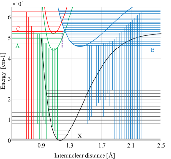
Figure 5: Vibronic structure of the MARVEL analysis. The vertical solid lines in green, blue and red illustrate the bands of $\upgamma$, $\upbeta$ and $\updelta$ systems, respectively. The vertical dash line in purple represents the $\mathrm{Heath}(0,0)$ band.

The spectroscopic network in MARVEL Furtenbacher, Császár, and Tennyson (2007b) is established in accordance with the upper and lower quantum numbers of the transitions. We used five quantum numbers, as shown in Table 3, to uniquely label the rovibronic energy levels. The quantum numbers of some transitions were improperly assigned. New assignments plus some other comments on the sources are given below:

• In some cases (e.g. for the $\mathrm{A}\,{}^{2}\Sigma^{+}$ state, the $Q_{21}$ branch is indeed a copy of $R_{11}$ branch as listed in 97DaDoKe Danielak et al. (1997)) duplicate transition are provided in source data. In 27JeBaMu Jenkins, Barton, and Mulliken (1927), 58LaMi Lagerqvist and Miescher (1958), etc., $\varLambda$ - doubling fine structures of many transitions are not resolved; therefore we simply created two transitions differing in $e/f$ parity with the same frequency in the MARVEL dataset.

• The uncertainties of the transitions of 27JeBaMu Jenkins, Barton, and Mulliken (1927) and 58LaMi Lagerqvist and Miescher (1958) were given by combination difference test, referring to the energies of $\mathrm{X}\,{}^{2}\Pi$ state Wong et al. (2017).

• The uncertainties of most validated transitions are close to the lower bounds listed in Table 2 (see the supplementary material).

• The transitions of $\upgamma(3,0)$, $\upbeta(6,0)$ and $\upbeta(11,0)$ bands extracted from 02ChLoLe Cheung et al. (2002), 02ChLoLe Cheung et al. (2002) and 02RuYoTh Rufus et al. (2002) were increased by $0.083\text{\,}{\mathrm{cm}}^{-1}$, $0.083\text{\,}{\mathrm{cm}}^{-1}$ and $0.067\text{\,}{\mathrm{cm}}^{-1}$, respectively, as suggested in 05ThRuYo Thorne et al. (2005). The uncertainties of these transitions should be $0.1\text{\,}{\mathrm{cm}}^{-1}$ because the absolute frequencies were not calibrated Thorne et al. (2005). However, we used relative accuracy, i.e., $0.03\text{\,}{\mathrm{cm}}^{-1}$, as the lower bound of uncertainty to constrain the MARVEL analysis. The uncertainties should be adjusted to $0.1\text{\,}{\mathrm{cm}}^{-1}$ if data of higher accuracy are included in the future.

• In the $\upbeta(10,0)$ band of 06YoThMu Yoshino et al. (2006), $R_{11}(3.5)$ and $P_{11}(3.5)$ were exchanged; the $R_{21}$ and $P_{21}$ branches were exchanged.

• In the $\updelta(0,0)$ band of 94MuYoEs Murray et al. (1994), $P_{12}(15.5)_{e}$ and $P_{12}(16.5)_{f}$ should be $P_{22}(15.5)_{e}$ and $P_{22}(16.5)_{e}$, respectively.

• In the $\updelta(1,0)$ band of 00ImYoEs Imajo et al. (2000), the frequencies of $R_{12}(15.5)_{e}$ and $R_{12}(15.5)_{f}$ should be exchanged; the frequencies of $P_{11}(5.5)$ and $P_{11}(16.5)_{f}$ should be $54\,668.636\text{\,}{\mathrm{cm}}^{-1}$.

• In the $\updelta(2,0)$ band of 06YoThMu Yoshino et al. (2006), the frequencies of $Q_{22}(5.5)_{e}$ and $Q_{22}(6.5)_{e}$ should be $56\,967.72$ and $56\,966.61\text{\,}{\mathrm{cm}}^{-1}$, respectively.

• The transitions, $R_{22}(0.5)_{ff}$, $Q_{22}(0.5)_{fe}$, $R_{12}(0.5)_{ee}$ of 97DaDoKe Danielak et al. (1997) and $R_{22}(0.5)$ of 02ChLoLe Cheung et al. (2002), are related to unknown lower states ($J=0.5$ and $\varOmega=1.5$). Those transitions were not validated.

The most serious issue we encountered concerned the 2020 measurements of Ventura and Fellows (20VeFeVentura and Fellows (2020)) who published a new line list for the $\upgamma$ system containing $6436$ transitions. The transitions of 20VeFe disagree with those measured by Danielak et al. (97DaDoKe) Danielak et al. (1997). MARVEL and combination difference analysis indicates that their data set is self-consistent within the claimed accuracy, i.e. $0.005\text{\,}{\mathrm{cm}}^{-1}0.06\text{\,}{\mathrm{cm}}^{-1}$. However, it is inconsistent with the ground state MARVEL energies of Wong et al. Wong et al. (2017). Combination difference test shows that the standard deviations of most energy levels calculated by the data set are greater than $0.1\text{\,}{\mathrm{cm}}^{-1}$.

In contrast, the line list of 97DaDoKe Danielak et al. (1997) is consistent with others. The measurements of 20VeFe differ from those of 97DaDoKeby up to $0.7\text{\,}{\mathrm{cm}}^{-1}$, as acknowledged by 20VeFe. The transitions $\upgamma(3,4)$ band measured by 97DaDoKe are consistent with the transitions in $\upgamma(3,0)$ band measured by Cheung et al. (02ChLoLe) Cheung et al. (2002). Furthermore, use of Heath band potential provides a closed loop or cycle by following $\upgamma(0,0)$-$\mathrm{Heath}(0,0)$-$\updelta(0,0)$. The measurements of 97DaDoKe gave consistency in this cycle, within the stated uncertainties of the various measurements, but 20VeFe did not. Analyzing the ground state data and 20VeFe individually, we observed an average $0.43\text{\,}{\mathrm{cm}}^{-1}$ shift for the lower three vibrational levels of the $\mathrm{A}\,{}^{2}\Sigma^{+}$ state; these energy differences are plotted in Fig. 6. We were therefore forced to conclude that the measurements of 20VeFe are not consistent with the other measurements and these data were excluded from our MARVEL analysis.

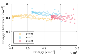
Figure 6: The differences between the $\mathrm{A}\,{}^{2}\Sigma^{+}$ state MARVEL energies corresponding to 20VeFe and those obtained from the sources of Table 2. The average energy shift is $0.43\text{\,}{\mathrm{cm}}^{-1}$.

Table 3: Quantum numbers used in the MARVEL analysis

Quan. No.	Meaning
State	Electronic state label, e.g., X stands for $\mathrm{X}\,{}^{2}\Pi$
$J$	Total angular momentum
parity	+ or -
$v$	Vibration quantum number
$\varOmega$	Projection of the total angular momentum on the internuclear axis

The $20\,293$ validated transitions (including $3141$ $\upgamma$, $4795$ $\upbeta$, $861$ $\updelta$ and $360$ Heath transitions) yielded $327$, $1400$ and $466$ energy levels of the $\mathrm{A}\,{}^{2}\Sigma^{+}$, $\mathrm{B}\,{}^{2}\Pi$ and $\mathrm{C}\,{}^{2}\Pi$ states, respectively. These levels are plotted as a function of total angular momentum $J$ in Fig. 7. The MARVEL transitions (input) file and energies (output) file are given as part of the supplementary data.

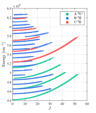
Figure 7: $\mathrm{A}\,{}^{2}\Sigma^{+}$, $\mathrm{B}\,{}^{2}\Pi$ and $\mathrm{C}\,{}^{2}\Pi$ state energy levels generated by MARVEL analysis.

Sulakshina and Borkov compared the ground state energies calculated by their RITZ code Sulakshina and Borkov (2018) with our previous MARVEL result Wong et al. (2017). The MARVEL analysis here updates the energy values of the $\mathrm{X}\,{}^{2}\Pi$ state by including new rovibronic transitions; as shown in Fig.8, the energy gaps between the results of the MARVEL and RITZ analysis are narrowed as a result of this. This is especially true for high $J$ levels belonging to the $\varOmega=\frac{3}{2}$ series (see Fig. 8(b) of Sulakshina and Borkov’s Sulakshina and Borkov (2018)). The majority of levels agree within the uncertainty of their determination.

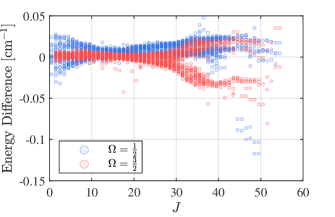
Figure 8: Energy difference of the $\mathrm{X}\,{}^{2}\Pi$ state between MARVEL result in this paper and the RITZ result in the work of Sulakshina and Borkov Sulakshina and Borkov (2018).

IV Refinement of curves for ^14N^16O

IV.1 Calculation setup

The PECs of $\mathrm{A}\,{}^{2}\Sigma^{+}$, $\mathrm{B}\,{}^{2}\Pi$ and $\mathrm{C}\,{}^{2}\Pi$, as well as other coupling curves, were refined based on the empirical energy levels yielded by the MARVEL analysis in Section III; the PEC for the $\mathrm{X}\,{}^{2}\Pi$ state was left unchanged from that of Wong et al. Wong et al. (2017) The refinement was executed in Duo  which is a general variational nuclear-motion program for calculating spectra of diatomic molecules Yurchenko et al. (2016).

Duo solves the diatomic molecular Schrödinger equation in two steps. Firstly the rotation-free radial equation of each electronic state is solved to get the vibrational energy levels, $E_{v}$, and wavefunctions, $\psi_{v}(r)$:

$$-\frac{\hbar^{2}}{2\mu}\frac{\mathrm{d}^{2}}{\mathrm{d}r^{2}}\psi_{v}(r)+V_{\mathrm{state}}(r)\psi_{v}(r)=E_{v}\psi_{v}(r)\,,$$ (1)

where $\mu$ is the reduced mass of the molecule and $V_{\mathrm{state}}(r)$ is the potential energy curve. This step creates vibrational basis functions, $\ket{\mathrm{state},v}$. Secondly, the fully-coupled, rovibronic Hamiltonian is diagonalized under the Hund’s case (a) rovibronic basis set defined by:

$$\ket{\mathrm{state},J,\varOmega,\varLambda,S,\varSigma,v}=\ket{\mathrm{state},\varLambda,S,\varSigma}\ket{J,\varOmega,M}\ket{\mathrm{state},v}\,,$$ (2)

where $\ket{\mathrm{state},\varLambda,S,\varSigma}$ and $\ket{J,\varOmega,M}$ represent the electronic and rotational basis functions, respectively.Tennyson et al. (2016b) The quantum number $M$ is the projection of the total angular momentum along the laboratory $Z$-axis.

Users are asked to set up some super-parameters to get the correct solution. The calculation setup for the refinement of ^14N^16O is summarized below. More details can be found in the Duo input file which is given as supplementary material and includes the PEC parameters.

• Equation (1) was solved by the Sinc-DVR method Colbert and Miller (1992).

• The calculation range was from 0.6 to 4.0 $\mathrm{\SIUnitSymbolAngstrom}$.

• The number of grids points was 701, uniformly spaced.

• The numbers of vibrational basis sets for $\mathrm{X}\,{}^{2}\Pi$, $\mathrm{A}\,{}^{2}\Sigma^{+}$, $\mathrm{B}\,{}^{2}\Pi$ and $\mathrm{C}\,{}^{2}\Pi$ were 10, 10, 30 and 10, respectively.

• The maximum total angular momentum considered here was $52\frac{1}{2}$.

• The upper bound of the total energy was $65\,000$ ${\mathrm{cm}}^{-1}$.

IV.2 Refinement results of the $\mathrm{A}\,{}^{2}\Sigma^{+}$ state

The PEC of $\mathrm{A}\,{}^{2}\Sigma^{+}$ state represented by a fourth-order Extended Morse Oscillator (EMO) function Lee et al. (1999). The EMO is defined as a function of internuclear distance, $r$:

$$V(r)=T_{\mathrm{e}}+\left(D_{\mathrm{e}}-T_{\mathrm{e}}\right)\left[1-\exp\left(-\beta_{\mathrm{EMO}}(r)\left(r-r_{\mathrm{e}}\right)\right)\right]^{2},$$ (3)

where the distance-dependent coefficient $\beta_{\mathrm{EMO}}$ is expressed as

$$\beta_{\mathrm{EMO}}(r)=\sum_{i=0}^{N}b_{i}y_{p}^{\mathrm{eq}}(r)^{i}.$$ (4)

The reduced variable $y_{p}^{\mathrm{eq}}(r)$ has the formula:

$$y_{p}^{\mathrm{eq}}(r)=\frac{r^{p}-(r_{\mathrm{e}})^{p}}{r^{p}+(r_{\mathrm{e}})^{p}}\,,$$ (5)

where $p$ controls the shape of $y_{p}^{\mathrm{eq}}(r)$. The programmed EMO function in Duo is not exactly the same as defined by Eq. 3. A reference point $R_{\mathrm{ref}}$ (usually the equilibrium internuclear distance) divides the curve into left and right parts. The numbers of terms $N$, as well as $p$, for the left and right parts can be assigned different values, i.e., $N_{\mathrm{L}}$, $N_{\mathrm{R}}$, $p_{\mathrm{L}}$ and $p_{\mathrm{R}}$. The unknown dissociation energy of the state is regarded as a dummy parameter in the refinement. The initial guess of $D_{e}$ was given by a pure Morse function and the value was fine-tuned in each iteration. The optimal parameters of the EMO function is listed in Table 4. The ab initio and refined PECs of the $\mathrm{A}\,{}^{2}\Sigma^{+}$ state are compared in Panel (a) of Fig. 9.

Table 4: The optimized EMO parameters of the PECs of $\mathrm{A}\,{}^{2}\Sigma^{+}$, $\mathrm{B}\,{}^{2}\Pi$, $\mathrm{C}\,{}^{2}\Pi$ states and the spin-orbit (SO) coupling within the $\mathrm{B}\,{}^{2}\Pi$ state. The pararmeters are given electronically in the Duo input which is given in the supplementary information.

Parameter	$\mathrm{A}\,{}^{2}\Sigma^{+}$	$\mathrm{B}\,{}^{2}\Pi$	$\mathrm{C}\,{}^{2}\Pi$	$\matrixelement{\mathrm{B}\,^{2}\Pi}{\hat{H}_{\mathrm{SO}}}{\mathrm{B}\,^{2}\Pi}$
$T_{\mathrm{e}}$ [${\mathrm{cm}}^{-1}$]	$4.390\,299\,277\,309\,43\text{\times}{10}^{04}$	$4.586\,704\,506\,760\,95\text{\times}{10}^{04}$	$5.208\,197\,358\,398\,84\text{\times}{10}^{04}$	$8.497\,424\,004\,318\,92\text{\times}{10}^{00}$
$r_{\mathrm{e}},r_{\mathrm{ref}}$ [$\mathrm{\SIUnitSymbolAngstrom}$]	$1.063\,666\,008\,368\,62$	$1.416\,639\,772\,450\,69$	$1.063\,704\,708\,372\,54$	$1.1$
$D_{\mathrm{e}}$ [${\mathrm{cm}}^{-1}$]	$1.292\,051\,390\,303\,94\text{\times}{10}^{05}$	$7.1627\text{\times}{10}^{04}$	$1.271\,773\,188\,884\,36\text{\times}{10}^{05}$	$5.774\,077\,920\,425\,91\text{\times}{10}^{01}$
$p$	$4$	$4$	$4$	$4$
$N_{\mathrm{l}}$	$2$	$4$	$2$	$4$
$N_{\mathrm{r}}$	$4$	$8$	$4$	$4$
$b_{0}$ [${\mathrm{\SIUnitSymbolAngstrom}}^{-1}$]	$2.704\,913\,981\,796\,78\text{\times}{10}^{00}$	$2.150\,144\,139\,754\,52\text{\times}{10}^{00}$	$2.863\,985\,603\,255\,24\text{\times}{10}^{00}$	$2.015\,987\,559\,388\,54\text{\times}{10}^{00}$
$b_{1}$ [${\mathrm{\SIUnitSymbolAngstrom}}^{-1}$]	$2.073\,903\,440\,604\,48\text{\times}{10}^{-02}$	$9.835\,900\,997\,934\,13\text{\times}{10}^{-02}$	$5.525\,275\,335\,431\,32\text{\times}{10}^{-01}$	$0$
$b_{2}$ [${\mathrm{\SIUnitSymbolAngstrom}}^{-1}$]	$8.149\,010\,097\,829\,77\text{\times}{10}^{-02}$	$4.118\,983\,730\,047\,04\text{\times}{10}^{-01}$	$3.452\,639\,965\,214\,17\text{\times}{10}^{00}$	$-3.768\,976\,845\,482\,42\text{\times}{10}^{00}$
$b_{3}$ [${\mathrm{\SIUnitSymbolAngstrom}}^{-1}$]	$-9.539\,702\,892\,896\,83\text{\times}{10}^{-01}$	$0$	$-3.788\,700\,193\,112\,05\text{\times}{10}^{01}$	$0$
$b_{4}$ [${\mathrm{\SIUnitSymbolAngstrom}}^{-1}$]	$2.050\,677\,385\,076\,37\text{\times}{10}^{00}$	$-4.436\,396\,750\,585\,21\text{\times}{10}^{-01}$	$8.286\,317\,439\,495\,08\text{\times}{10}^{01}$	$6.672\,511\,527\,886\,65\text{\times}{10}^{00}$
$b_{5}$ [${\mathrm{\SIUnitSymbolAngstrom}}^{-1}$]		$1.215\,719\,272\,327\,52\text{\times}{10}^{01}$
$b_{6}$ [${\mathrm{\SIUnitSymbolAngstrom}}^{-1}$]		$-1.784\,795\,357\,577\,77\text{\times}{10}^{01}$
$b_{7}$ [${\mathrm{\SIUnitSymbolAngstrom}}^{-1}$]		$3.127\,784\,544\,525\,73\text{\times}{10}^{00}$
$b_{8}$ [${\mathrm{\SIUnitSymbolAngstrom}}^{-1}$]		$5.403\,077\,729\,588\,00\text{\times}{10}^{00}$

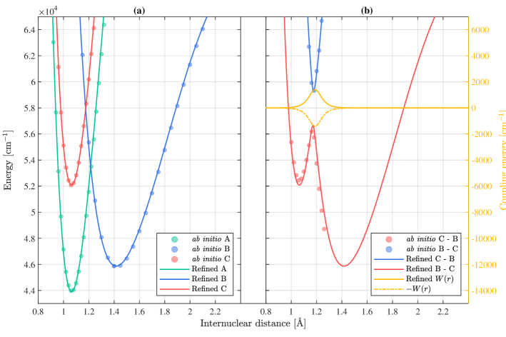
Figure 9: The ab initio and refined PECs of the $\mathrm{A}\,{}^{2}\Sigma^{+}$, $\mathrm{B}\,{}^{2}\Pi$ and $\mathrm{C}\,{}^{2}\Pi$ states as well as the refined B - C interaction term $W(r)$. (a) diabatic and (b) adiabatic representations. The refined potential curves in Panel (b) is calculated using Eqs. (10) and (11). The ab initio curves are shifted using empirical $T_{e}$ values.

In addition, our model of the $\mathrm{A}\,{}^{2}\Sigma^{+}$ state contains a spin-rotational term. In Duo, the nonzero diagonal and off-diagonal matrix elements of spin-rotational operator ${\hat{H}_{\mathrm{SR}}}$Tennyson et al. (2016b) are given by

$$\matrixelement{\varLambda,S,\varSigma}{\hat{H}_{\mathrm{SR}}}{\varLambda,S,\varSigma} \,=\frac{\hbar^{2}}{2\mu r^{2}}\gamma^{\mathrm{SR}}(r)\left[\varSigma^{2}-S(S+1)\right]\,,$$ (6)

$$\matrixelement{\varLambda,S,\varSigma}{\hat{H}_{\mathrm{SR}}}{\varLambda,S,\varSigma\pm 1} \,=\frac{\hbar^{2}}{4\mu r^{2}}\gamma^{\mathrm{SR}}(r)\sqrt{S(S+1)-\varSigma(\varSigma\pm 1)}$$

$$\quad\times\sqrt{J(J+1)-\varOmega(\varOmega\pm 1)}\,.$$ (7)

The dimensionless spin-rotational coefficient $\gamma^{\mathrm{SR}}(r)$ of $\mathrm{A}\,{}^{2}\Sigma^{+}$ state was modeled as a constant whose value is

$$\gamma^{\mathrm{SR}}_{\mathrm{A}}(r)=$-2.080\,430\,044\,787\,81\text{\times}{10}^{-03}$\,.$$ (8)

IV.3 Refinement results of the $\mathrm{B}\,{}^{2}\Pi$  - $\mathrm{C}\,{}^{2}\Pi$ coupled states

IV.3.1 Deperturbation of the $\mathrm{B}\,{}^{2}\Pi$  - $\mathrm{C}\,{}^{2}\Pi$ interaction

For this work we only consider coupling between two electronic states. The interaction between two electronic states belong to the same irreducible representation of the molecular point group directly depends on the avoided crossing of their diabatic PECs. Thus, it is possible to model the coupled states by introducing two adiabatic potentials Karman et al. (2018). This could be accomplished by diagonalizing the matrix:

$$\begin{pmatrix}V_{1}(r)&W(r)\\ W(r)&V_{2}(r)\end{pmatrix}\,,$$ (9)

where $V_{1}(r)$ and $V_{2}(r)$ are two diabatic potentials and $W(r)$ is the coupling curves. The adiabatic PECs, i.e. the eigenvalues of the matrix, are

$$V_{\text{low }}(r) =\frac{V_{1}(r)+V_{2}(r)}{2}-\frac{\sqrt{\left[V_{1}(r)-V_{2}(r)\right]^{2}+4W^{2}(r)}}{2}\,,$$ (10)

$$V_{\text{upp }}(r) =\frac{V_{1}(r)+V_{2}(r)}{2}+\frac{\sqrt{\left[V_{1}(r)-V_{2}(r)\right]^{2}+4W^{2}(r)}}{2}\,.$$ (11)

EMO potential functions are used to model $V_{1}(r)$ and $V_{2}(r)$ in Eqs. (10) and (11) while $W(r)$ is given by:

$$W(r)=\frac{\sum_{i\geq 0}w_{i}\left(r-r_{0}\right)^{i}}{\cosh\left(b\left(r-r_{0}\right)\right)}\,.$$ (12)

The function rapidly decreases to $W_{0}$ when $r$ moves away from $r_{0}$.

The coupled PECs of $\mathrm{X}\,^{1}\Sigma_{\mathrm{g}}^{+}$ and $\mathrm{B}^{\prime}\,{}^{1}\Sigma_{\mathrm{g}}^{+}$ states of C_2 were represented by adiabatic potential in our previous work Yurchenko et al. (2018), producing accurate line list. Nevertheless, this method is not optimal for NO where the avoided crossing between the B and C states is very sharp. Thus, for example, the adiabatic B – X and C – X transition dipole moment curves (TDMCs) change dramatically around the crossing point making them hard to use in any reliable calculation of transition intensities and a slight shift of the crossing point, $r_{0}$, during refinement may significantly change the intensities of nearby lines. We therefore adopt the following procedure for the generating line lists involving these coupled electronic states:

1. Solve the radial equations set up with diabatic PECs of different electronic states to get vibrational basis.

2. Construct rovibronic Hamiltonian matrix with all necessary elements, including the electronic interaction terms.

3. Diagonalize the matrix under rovibronic basis set to get the rovibronic energy levels and the corresponding wavefunctions.

4. Refine the diabatic PECs, electronic interaction terms and other coupling curves by fitting the energies to observed energy levels.

5. Calculate the Einstein A coefficient with the diabatic TDMCs and let the wavefunctions determine the weights of TDMCs for each rovibronic state at different geometries.

The method not only rescues us from the dilemma of constructing adiabatic TDMCs but also improves the flexibility of our program. For instance, it is convenient to model the $\mathrm{B}\,{}^{2}\Pi$  - $\mathrm{C}\,{}^{2}\Pi$  - $\mathrm{L}\,{}^{2}\Pi$ coupled states of NO by adding new definitions of the potential of $\mathrm{L}\,{}^{2}\Pi$ and coupled term between $\mathrm{C}\,{}^{2}\Pi$ and $\mathrm{L}\,{}^{2}\Pi$ in the input file of Duo, without changing its code.

IV.3.2 Refined curves

The diabatic PECs of $\mathrm{B}\,{}^{2}\Pi$ and $\mathrm{C}\,{}^{2}\Pi$ states were modeled using EMO functions whose optimal parameters are listed in Table 4. The ab initio and refined PECs of $\mathrm{B}\,{}^{2}\Pi$ and $\mathrm{C}\,{}^{2}\Pi$ states are compared in Panel (a) Fig. 9. Its optimal parameters of the function are listed in Table 5. Although not used in this work, the adiabatic curves were calculated as defined by Eqs. (10) and (11). They are compared with the ab initio adiabatic PECs in Panel (b) of Fig. 9. The dissociation energy of $\mathrm{C}\,{}^{2}\Pi$ state is also a dummy parameter. The refined PECs of $\mathrm{A}\,{}^{2}\Sigma^{+}$ and $\mathrm{C}\,{}^{2}\Pi$ states are physically meaningless outside the our calculation range (i.e., when energy is greater than $73\,000\text{\,}{\mathrm{cm}}^{-1}$).

Table 5: Optimized Lorentz parameters for the B - C interaction curve.

Parameter	Value
$b$ [${\mathrm{\SIUnitSymbolAngstrom}}^{-1}$]	$2.217\,076\,306\,467\,40\text{\times}{10}^{01}$
$r_{0}$ [$\mathrm{\SIUnitSymbolAngstrom}$]	$1.188\,085\,737\,226\,98$
$w_{0}$ [${\mathrm{cm}}^{-1}$]	$1.401\,731\,787\,542\,00\text{\times}{10}^{03}$

The spin-orbit coupling curve (SOC) of $\mathrm{B}\,{}^{2}\Pi$ state was also fitted to an EMO function whose optimal parameters are listed in the last column of Table 4. Figure 10 compares the ab initio and refined SOCs. The diagonal spin-orbital term of $\mathrm{C}\,{}^{2}\Pi$ state and the off-diagonal term between $\mathrm{B}\,{}^{2}\Pi$ and $\mathrm{C}\,{}^{2}\Pi$ were determined empirically by fitting to constants. The spin-rotational coefficient of $\mathrm{C}\,{}^{2}\Pi$ state was also model on a constant. The values of these terms are listed in Table 6.

Table 6: Optimized values of the spin-orbit (SO) and spin-rotation (SR) coupling terms.

Term	Value
$\matrixelement{\mathrm{C}\,^{2}\Pi}{\hat{H}_{\mathrm{SO}}}{\mathrm{C}\,^{2}\Pi}$ [$\mathrm{c}\mathrm{m}^{-1}$]	$1.817\,667\,722\,287\,87\text{\times}{10}^{00}$
$\matrixelement{\mathrm{C}\,^{2}\Pi}{\hat{H}_{\mathrm{SO}}}{\mathrm{B}\,^{2}\Pi}$ [${\mathrm{cm}}^{-1}$]	$2.282\,063\,757\,469\,38\text{\times}{10}^{00}$
$\quad\gamma_{\mathrm{C}}^{\mathrm{SR}}$	$2.705\,930\,617\,891\,97\text{\times}{10}^{-03}$

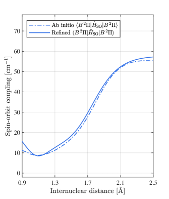
Figure 10: The spin-orbit coupling curves of $\mathrm{B}\,{}^{2}\Pi$ states.

The $\varLambda$ - doubling fine structures of $\upbeta$ and $\updelta$ system bands were observed in most of the work listed in Table 2. Duo calculates the $\varLambda$ - doubling matrix elements, i.e., $\matrixelement{\varLambda^{\prime}\varSigma^{\prime}J^{\prime}\varOmega^{\prime}}{\hat{H}_{\mathrm{LD}}}{\varLambda^{\prime\prime}\varSigma^{\prime\prime}J^{\prime\prime}\varOmega^{\prime\prime}}$, according to the terms given by Brown and Merer, Brown and Merer (1979):

$$\matrixelement{\mp 1,\varSigma\pm 2,J,\varOmega}{\hat{H}_{\mathrm{LD}}}{\pm 1,\varSigma,J,\varOmega}=\frac{1}{2}\left(o_{v}+p_{v}+q_{v}\right)\times$$

$$\quad\sqrt{[S(S+1)-\varSigma(\varSigma\pm 1)][S(S+1)-(\varSigma\pm 1)(\varSigma\pm 2)]}\,,$$ (13)

$$\matrixelement{\mp 1,\varSigma\pm 1,J,\varOmega\mp 1}{\hat{H}_{\mathrm{LD}}}{\pm 1,\varSigma,J,\varOmega}=-\frac{1}{2}\left(p_{v}+2q_{v}\right)\times$$

$$\quad\sqrt{[S(S+1)-\varSigma(\varSigma\pm 1)][J(J+1)-\varOmega(\varOmega\mp 1)]}\,,$$ (14)

$$\matrixelement{\mp 1,\varSigma,J,\varOmega\mp 2}{\hat{H}_{\mathrm{LD}}}{\pm 1,\varSigma,J,\varOmega}=\frac{1}{2}q_{v}\times$$

$$\quad\sqrt{[J(J+1)-\varOmega(\varOmega\mp 1)][J(J+1)-(\varOmega\mp 1)(\varOmega\mp 2)]}\,.$$ (15)

For $\mathrm{B}\,{}^{2}\Pi$ and $\mathrm{C}\,{}^{2}\Pi$, $\varSigma=\pm 1/2$. Therefore, the matrix elements described in Eq. (13) are zero and only the coefficient curves of Eqs. (14) and (15) were fitted to polynomials, i.e.,

$$P(r)=a_{0}+\sum_{i\geq 0}a_{i}(r-r_{0})^{i}.$$ (16)

The optimized parameters of the $\varLambda$ - doubling terms are listed in Table 7.

Table 7: Optimized polynomial parameters of the $\varLambda$ - doubling curves of the $\mathrm{B}\,{}^{2}\Pi$ and $\mathrm{C}\,{}^{2}\Pi$ states

Parameter	$\mathrm{B}\,{}^{2}\Pi$		$\mathrm{C}\,{}^{2}\Pi$
	$p_{v}+2q_{v}$	$q_{v}$	$p_{v}+2q_{v}$	$q_{v}$
$r_{\mathrm{0}}$ [$\mathrm{\SIUnitSymbolAngstrom}$]	$1.416\,504\,703\,523\,37\text{\times}{10}^{00}$	$1.416\,504\,703\,523\,37\text{\times}{10}^{00}$	$0$	$1.064\,436\,059\,412\,32\text{\times}{10}^{00}$
$a_{0}$ [${\mathrm{cm}}^{-1}$]	$1.065\,516\,703\,466\,50\text{\times}{10}^{-02}$	$6.453\,326\,916\,333\,86\text{\times}{10}^{-05}$	$-3.660\,394\,013\,643\,46\text{\times}{10}^{-02}$	$-1.612\,437\,381\,504\,96\text{\times}{10}^{-02}$
$a_{1}$ [${\mathrm{cm}}^{-1}\text{\,}{\mathrm{\SIUnitSymbolAngstrom}}^{-1}$]	$-2.921\,142\,813\,629\,27\text{\times}{10}^{-01}$	$-1.189\,741\,089\,831\,74\text{\times}{10}^{-02}$	$0$	$3.003\,216\,097\,917\,86\text{\times}{10}^{-02}$
$a_{2}$ [$\mathrm{c}\mathrm{m}^{-1}\mathrm{\SIUnitSymbolAngstrom}^{-2}$]	$5.095\,170\,164\,836\,91\text{\times}{10}^{-01}$	$3.040\,771\,809\,152\,39\text{\times}{10}^{-02}$	$0$	$0$

IV.3.3 Fitting residues of the rovibronic energy levels

The fitting residues of the $\mathrm{A}\,{}^{2}\Sigma^{+}$ state are shown in Panel (a) of Fig. 11. The high-$J$ energies of $v=3$ vibrational levels are mainly determined by blended lines of 97DaDoKe.NO Danielak et al. (1997). The fitting residues of the $\mathrm{B}\,{}^{2}\Pi$ and $\mathrm{C}\,{}^{2}\Pi$ states are shown in Panel (b) of Fig. 11, where the cold colors represent the $\mathrm{B}\,{}^{2}\Pi$ state and the warm ones represent the $\mathrm{C}\,{}^{2}\Pi$ state. The $F_{1}$ (i.e., $\varOmega=\frac{1}{2}$) and $F_{2}$ (i.e., $\varOmega=\frac{3}{2}$) levels are also distinguishable. The residue distributions indicate $J$-dependent systematic error of our model, which may result from some off-diagonal couplings, e.g., the coupling between $\mathrm{C}\,{}^{2}\Pi$ and $\mathrm{D}\,{}^{2}\Sigma^{+}$ states Amiot and Verges (1982).

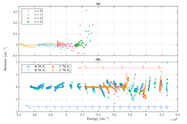
Figure 11: Fitting residues of (a) $\mathrm{A}\,{}^{2}\Sigma^{+}$ state and (b) $\mathrm{B}\,{}^{2}\Pi$  - $\mathrm{C}\,{}^{2}\Pi$ coupled states.

The residues of all rovibronic energy levels are plotted against their corresponding uncertainties. The root-mean-square and average value of uncertainties and residues are compared in Table 8.

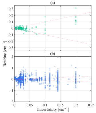
Figure 12: Residues against uncertainties of (a) $\mathrm{A}\,{}^{2}\Sigma^{+}$ state and (b) B - C coupled states with vibrational states given in the bars.

Table 8: Overall comparison of uncertainty and residue.

All in ${\mathrm{cm}}^{-1}$	$\mathrm{A}\,{}^{2}\Sigma^{+}$	$\mathrm{B}\,{}^{2}\Pi$  - $\mathrm{C}\,{}^{2}\Pi$
RMS uncertainty	0.04284	0.07927
RMS residue	0.03390	0.27217
Average uncertainty	0.02453	0.05753
Average absolute residue	0.01599	0.18603

The accuracy of our model is definitely higher than those of Lagerqvist and Miescher Lagerqvist and Miescher (1958), or Gallusser and Dressler Gallusser and Dressler (1982), On one hand, the most recent measurements (e.g., the works of Yoshino et al. Yoshino et al. (2006)) and spectroscopic analysis techniques (MARVEL Furtenbacher, Császár, and Tennyson (2007b)) helped us reconstruct reliable spectroscopic network and energy levels. On the other hand, our model was directly fitted to the observed rovibronic levels. The vibronic residues given by Gallusser and Dressler Gallusser and Dressler (1982) are greater than our rovibronic residues. Unlike Gallusser and Dressler, we did not include higher electronic states, such as $\mathrm{L}\,{}^{2}\Pi$ and $\mathrm{K}\,{}^{2}\Pi$, in our model, which reduces its range of applicability where the state energy is greater than $63\,000\text{\,}{\mathrm{cm}}^{-1}$. However, thanks to diabatic coupling strategy of Duo, the model can easily be updated in a future study.

We note that some of the assignments to B or C electronic states differ between Duo and our MARVEL analysis. Duo uses three good quantum number, namely the total angular momentum $J$, the total parity and the counting number of the levels with the same values of $J$ and parity. The other quantum numbers such as state, $v$, $\varOmega$, are estimated using the contribution of the basis functions to a given wavefunction. It is to be anticipated that in regions of heavily mixed wavefunctions this may lead to differences compared to other assignment methods. The MARVEL and Duo energy levels of B ($v=13$) - C ($v=2$) coupled series are plotted in Fig. 13. Table 9 lists some energy levels in the output .en file of Duo. Both of them demonstrate the differences between the quantum numbers of MARVEL and Duo results.

Figure 13: Calculated and observed energy levels of the $\mathrm{B}(v=13)$ - $\mathrm{C}(v=2)$ coupled series. The right hand panel is a blow up of the avoided crossing between the states which gives a clearer view of the $\varLambda$ - doubling splitting and the difference between the quantum numbers given by MARVEL and Duo.

Table 9: Sample lines extracted from the output .en file of Duo.

Duo	Assigned			MARVEL	Duo			Duo					MARVEL
$N$	$N$	$J$	Parity	Energy	Energy	Residue	Weight	state	$v$	$\varLambda$	$\varSigma$	$\varOmega$	state	$v$	$\varLambda$	$\varSigma$	$\varOmega$
39	39	1.5	+	52349.0418	52349.0274	0.0144	9.50E-05	3	7	1	-0.5	0.5	3	7	1	-0.5	0.5
40	40	1.5	+	52373.2372	52373.3626	-0.1255	1.40E-03	4	0	1	0.5	1.5	3	7	1	0.5	1.5
41	41	1.5	+	52380.1912	52380.1101	0.0810	1.30E-03	4	0	1	-0.5	0.5	4	0	1	-0.5	0.5
42	42	1.5	+	52392.3007	52392.3172	-0.0165	1.30E-03	3	7	1	0.5	1.5	4	0	1	0.5	1.5
64	64	2.5	-	59217.4976	59217.9730	-0.4754	9.50E-05	3	15	-1	0.5	-0.5	4	3	-1	0.5	-0.5
65	65	2.5	-	59250.3720	59250.8248	-0.4528	9.50E-05	4	3	-1	-0.5	-1.5	4	3	-1	-0.5	-1.5
66	66	2.5	-	59654.3005	59654.8551	-0.5546	3.70E-06	4	3	-1	0.5	-0.5	3	15	-1	0.5	-0.5
67	67	2.5	-	59692.2845	59692.6292	-0.3447	4.80E-06	3	15	-1	-0.5	-1.5	3	15	-1	-0.5	-1.5

V Conclusion

In this paper, potential energy curves and coupling for the low-lying electronic state of NO are calculated using quantum chemistry package Molpro. The strong interaction between Rydberg and valence states makes the ab initio calculation challenging. We obtain both adiabatic and diabatic PECs and SOCs for the $\mathrm{A}\,{}^{2}\Sigma^{+}$, $\mathrm{B}\,{}^{2}\Pi$ and $\mathrm{C}\,{}^{2}\Pi$ states. The curves were refined by fitting the rovibronic energy levels calculated by variational nuclear motion program Duo to those reconstructed by MARVEL analysis. The RMS error of the $\mathrm{A}\,{}^{2}\Sigma^{+}$ state fitting and $\mathrm{B}\,{}^{2}\Pi$  - $\mathrm{C}\,{}^{2}\Pi$ coupled states fitting are $0.033\,90\text{\,}{\mathrm{cm}}^{-1}$ and $0.272\,17\text{\,}{\mathrm{cm}}^{-1}$, respectively, which energies were determined by our use of a MARVEL procedure and the best available measurements. The success of $\mathrm{B}\,{}^{2}\Pi$  - $\mathrm{C}\,{}^{2}\Pi$ coupled states fitting validates our deperturbation method for treating the coupled electronic state. This work, when combined with the earlier $\mathrm{X}\,{}^{2}\Pi$ study of Wang et al.,Wong et al. (2017) provides a comprehensive spectroscopic model four the lowest for electronic states of NO and thus a good start point for the generation of a NO UV line list. This line list will be presented elsewhere.

Data Availability

The data that supports the findings of this study are available within the article and its supplementary material.

Supplementary material

Three text files are provided as supplementary material to the article:
MARVEL_Transitions.txt: input transitions file used with MARVEL.
MARVEL_Energies.txt: energy levels file generated by MARVEL using the file MARVEL_Transitions.txt.
NO_XABC.model.txt: a Duo input file which full specifies our spectroscopic model including the associated potential energy and coupling curves.

References

- Canfield, Glazer, and Falkowski (2010) D. E. Canfield, A. N. Glazer, and P. G. Falkowski, Science 330, 192 (2010).
- Vitousek et al. (1997) P. M. Vitousek, J. D. Aber, R. W. Howarth, G. E. Likens, P. A. Matson, D. W. Schindler, W. H. Schlesinger, and D. G. Tilman, Ecol. Appl. 7, 737 (1997).
- Chameides et al. (1994) W. L. Chameides, P. S. Kasibhatla, J. Yienger, and H. Levy, Science 264, 74 (1994).
- Likens, Driscoll, and Buso (1996) G. E. Likens, C. T. Driscoll, and D. C. Buso, Science 272, 244 (1996).
- Singh and Agrawal (2007) A. Singh and M. Agrawal, J. Environ. Biol. 29, 15 (2007).
- Hu et al. (2000) Y. Hu, S. Naito, N. Kobayashi, and M. Hasatani, Fuel 79, 1925 (2000).
- Li, Lu, and Rudolph (1998) Y. Li, G. Lu, and V. Rudolph, Chem. Eng. Sci. 53, 1 (1998).
- Bredt and Snyder (1992) D. S. Bredt and S. H. Snyder, Neuron 8, 3 (1992).
- Bredt and Snyder (1994) D. S. Bredt and S. H. Snyder, Annu. Rev. Biochem. 63, 175 (1994).
- Arasimowicz and Floryszak-Wieczorek (2007) M. Arasimowicz and J. Floryszak-Wieczorek, Plant Sci. 172, 876 (2007).
- Mayer and Hemmens (1997) B. Mayer and B. Hemmens, Trends Biochem. Sci. 22, 477 (1997).
- Estévez and Jordán (2002) A. G. Estévez and J. Jordán, Ann. N.Y. Acad. Sci. 962, 207 (2002).
- Ziurys et al. (1991) L. M. Ziurys, D. McGonagle, Y. Minh, and W. M. Irvine, Astrophys. J. 373, 535 (1991).
- Cox et al. (2008) C. Cox, A. Saglam, J.-C. Gerard, J.-L. Bertaux, F. Gonzalez-Galindo, F. Leblanc, and A. Reberac, J. Geophys. Res.-Planets 113, E08012 (2008).
- Gérard et al. (2008) J.-C. Gérard, C. Cox, A. Saglam, J.-L. Bertaux, E. Villard, and C. Nehmé, J. Geophys. Res. 113, E00B03 (2008).
- Gérard et al. (2009) J.-C. Gérard, C. Cox, L. Soret, A. Saglam, G. Piccioni, J.-L. Bertaux, and P. Drossart, J. Geophys. Res. 114, E00B44 (2009).
- Partington (1936) J. Partington, Ann. Sci. 1, 359 (1936).
- Priestley (1772) J. Priestley, Philos. Trans. R. Soc. Lond. 62, 147 (1772).
- Deller and Hogan (2020) A. Deller and S. D. Hogan, J. Chem. Phys. 152, 144305 (2020).
- Bessler and Schulz (2004) W. G. Bessler and C. Schulz, Appl. Phys. B-Lasers Opt. 78, 519 (2004).
- Van Gessel et al. (2013) A. F. Van Gessel, B. Hrycak, M. Jasiński, J. Mizeraczyk, J. J. Van Der Mullen, and P. J. Bruggeman, J. Phys. D-Appl. Phys. 46, 095201 (2013).
- Tennyson and Yurchenko (2012) J. Tennyson and S. N. Yurchenko, Mon. Not. Roy. Astron. Soc. 425, 21 (2012).
- Tennyson et al. (2016a) J. Tennyson, S. N. Yurchenko, A. F. Al-Refaie, E. J. Barton, K. L. Chubb, P. A. Coles, S. Diamantopoulou, M. N. Gorman, C. Hill, A. Z. Lam, L. Lodi, L. K. McKemmish, Y. Na, A. Owens, O. L. Polyansky, T. Rivlin, C. Sousa-Silva, D. S. Underwood, A. Yachmenev, and E. Zak, J. Mol. Spectrosc. 327, 73 (2016a).
- Tennyson et al. (2020) J. Tennyson, S. N. Yurchenko, A. F. Al-Refaie, V. H. J. Clark, K. L. Chubb, E. K. Conway, A. Dewan, M. N. Gorman, C. Hill, A. E. Lynas-Gray, T. Mellor, L. K. McKemmish, A. Owens, O. L. Polyansky, M. Semenov, W. Somogyi, G. Tinetti, A. Upadhyay, I. Waldmann, Y. Wang, S. Wright, and O. P. Yurchenko, J. Quant. Spectrosc. Radiat. Transf. 255, 107228 (2020).
- Wong et al. (2017) A. Wong, S. N. Yurchenko, P. Bernath, H. S. P. Mueller, S. McConkey, and J. Tennyson, Mon. Not. Roy. Astron. Soc. 470, 882 (2017).
- Lagerqvist and Miescher (1958) A. Lagerqvist and E. Miescher, Helv. Phys. Acta 31, 221 (1958).
- Danielak et al. (1997) J. Danielak, U. Domin, R. Kepa, M. Rytel, and M. Zachwieja, J. Mol. Spectrosc. 181, 394 (1997).
- Yoshino et al. (2006) K. Yoshino, A. P. Thorne, J. E. Murray, A. S.-C. Cheung, A. L. Wong, and T. Imajo, J. Chem. Phys. 124, 054323 (2006).
- Gordon et al. (2017) I. E. Gordon, L. S. Rothman, C. Hill, R. V. Kochanov, Y. Tan, P. F. Bernath, M. Birk, V. Boudon, A. Campargue, K. V. Chance, B. J. Drouin, J.-M. Flaud, R. R. Gamache, J. T. Hodges, D. Jacquemart, V. I. Perevalov, A. Perrin, K. P. Shine, M.-A. H. Smith, J. Tennyson, G. C. Toon, H. Tran, V. G. Tyuterev, A. Barbe, A. G. Császár, V. M. Devi, T. Furtenbacher, J. J. Harrison, J.-M. Hartmann, A. Jolly, T. J. Johnson, T. Karman, I. Kleiner, A. A. Kyuberis, J. Loos, O. M. Lyulin, S. T. Massie, S. N. Mikhailenko, N. Moazzen-Ahmadi, H. S. P. Müller, O. V. Naumenko, A. V. Nikitin, O. L. Polyansky, M. Rey, M. Rotger, S. W. Sharpe, K. Sung, E. Starikova, S. A. Tashkun, J. Vander Auwera, G. Wagner, J. Wilzewski, P. Wcisło, S. Yu, and E. J. Zak, J. Quant. Spectrosc. Radiat. Transf. 203, 3 (2017).
- Jacquinet-Husson et al. (2016) N. Jacquinet-Husson, R. Armante, N. A. Scott, A. Chédin, L. Crépeau, C. Boutammine, A. Bouhdaoui, C. Crevoisier, V. Capelle, C. Boonne, N. Poulet-Crovisier, A. Barbe, D. C. Benner, V. Boudon, L. R. Brown, J. Buldyreva, A. Campargue, L. H. Coudert, V. M. Devi, M. J. Down, B. J. Drouin, A. Fayt, C. Fittschen, J.-M. Flaud, R. R. Gamache, J. J. Harrison, C. Hill, Ø. Hodnebrog, S. M. Hu, D. Jacquemart, A. Jolly, E. Jiménez, N. N. Lavrentieva, A. W. Liu, L. Lodi, O. M. Lyulin, S. T. Massie, S. Mikhailenko, H. S. P. Müller, O. V. Naumenko, A. Nikitin, C. J. Nielsen, J. Orphal, V. I. Perevalov, A. Perrin, E. Polovtseva, A. Predoi-Cross, M. Rotger, A. A. Ruth, S. S. Yu, K. Sung, S. A. Tashkun, J. Tennyson, V. G. Tyuterev, J. Vander Auwera, B. A. Voronin, and A. Makie, J. Mol. Spectrosc. 327, 31 (2016).
- Luque and Crosley (1995) J. Luque and D. R. Crosley, J. Quant. Spectrosc. Radiat. Transf. 53, 189 (1995).
- Luque and Crosley (1999a) J. Luque and D. R. Crosley, J. Chem. Phys. 111, 7405 (1999a).
- Luque and Crosley (2000) J. Luque and D. R. Crosley, J. Chem. Phys. 112, 9411 (2000).
- Luque and Crosley (1999b) J. Luque and D. R. Crosley, SRI international report MP 99 (1999b).
- Yoshino et al. (1998) K. Yoshino, J. R. Esmond, W. H. Parkinson, A. P. Thorne, J. E. Murray, R. C. M. Learner, G. Cox, A. S.-C. Cheung, K. W.-S. Leung, K. Ito, T. Matsui, and T. Imajo, J. Chem. Phys. 109, 1751 (1998).
- Albritton, Schmeltekopf, and Zare (1979) D. L. Albritton, A. L. Schmeltekopf, and R. N. Zare, The Journal of Chemical Physics 71, 3271 (1979).
- Gallusser and Dressler (1982) R. Gallusser and K. Dressler, J. Chem. Phys. 76, 4311 (1982).
- Furtenbacher, Császár, and Tennyson (2007a) T. Furtenbacher, A. G. Császár, and J. Tennyson, J. Mol. Spectrosc. 245, 115 (2007a).
- Tóbiás et al. (2019) R. Tóbiás, T. Furtenbacher, J. Tennyson, and A. G. Császár, Phys. Chem. Chem. Phys. 21, 3473 (2019).
- Werner et al. (2015) H. J. Werner, P. J. Knowles, G. Knizia, F. R. Manby, M. Schütz, P. Celani, W. Győrffy, D. Kats, T. Korona, R. Lindh, A. Mitrushenkov, G. Rauhut, K. R. Shamasundar, T. B. Adler, R. D. Amos, A. Bernhardsson, A. Berning, D. L. Cooper, M. J. O. Deegan, A. J. Dobbyn, F. Eckert, E. Goll, C. Hampel, A. Hesselmann, G. Hetzer, T. Hrenar, G. Jansen, C. Köppl, Y. Liu, A. W. Lloyd, R. A. Mata, A. J. May, S. J. McNicholas, W. Meyer, M. E. Mura, A. Nicklass, D. P. O’Neill, P. Palmieri, D. Peng, K. Pflüger, R. Pitzer, M. Reiher, T. Shiozaki, H. Stoll, A. J. Stone, R. Tarroni, T. Thorsteinsson, and M. Wang, “Molpro, version 2015.1, a package of ab initio programs,” http://www.molpro.net (2015).
- Jenkins, Barton, and Mulliken (1927) F. A. Jenkins, H. A. Barton, and R. S. Mulliken, Phys. Rev. 30, 150 (1927).
- Amiot (1982) C. Amiot, J. Mol. Spectrosc. 94, 150 (1982).
- Cartwright et al. (2000) D. C. Cartwright, M. J. Brunger, L. Campbell, B. Mojarrabi, and P. J. O. Teubner, J. Geophys. Res. 105, 20857 (2000).
- Werner et al. (2012) H.-J. Werner, P. J. Knowles, G. Knizia, F. R. Manby, and M. Schütz, WIREs Comput. Mol. Sci. 2, 242 (2012).
- Grein and Kapur (1982) F. Grein and A. Kapur, J. Chem. Phys. 77, 415 (1982).
- Devivie and Peyerimhoff (1988) R. Devivie and S. D. Peyerimhoff, J. Chem. Phys. 89, 3028 (1988).
- Shi and East (2006) H. Shi and A. L. L. East, J. Chem. Phys. 125, 7 (2006).
- Cheng, Zhang, and Cheng (2017) J. Cheng, H. Zhang, and X. Cheng, Comput. Theor. Chem. 1114, 165 (2017).
- Cheng et al. (2017) J. Cheng, H. Zhang, X. Cheng, and X. Song, Mol. Phys. 115, 2577 (2017).
- Cooper (1982) D. M. Cooper, J. Quant. Spectrosc. Radiat. Transf. 27, 459 (1982).
- Langhoff, Bauschlicher, and Partridge (1988) S. R. Langhoff, C. W. Bauschlicher, and H. Partridge, J. Chem. Phys. 89, 4909 (1988).
- Langhoff et al. (1991) S. R. Langhoff, H. Partridge, C. W. Bauschlicher, and A. Komornicki, J. Chem. Phys. 94, 6638 (1991).
- Polak and Fiser (2003) R. Polak and J. Fiser, Chem. Phys. Lett. 377, 564 (2003).
- Dunning (1989) T. H. Dunning, J. Chem. Phys. 90, 1007 (1989).
- Huber and Herzberg (1979) K. P. Huber and G. Herzberg, Molecular Spectra and Molecular Structure IV. Constants of Diatomic Molecules (Van Nostrand Reinhold Company, New York, 1979).
- Murray et al. (1994) J. E. Murray, K. Yoshino, J. R. Esmond, W. H. Parkinson, Y. Sun, A. Dalgarno, A. P. Thorne, and G. Cox, J. Chem. Phys. 101, 62 (1994).
- Imajo et al. (2000) T. Imajo, K. Yoshino, J. R. Esmond, W. H. Parkinson, A. P. Thorne, J. E. Murray, R. C. M. Learner, G. Cox, A. S.-C. Cheung, K. Ito, and T. Matsui, J. Chem. Phys. 112, 2251 (2000).
- Cheung et al. (2002) A. S.-C. Cheung, D. H.-Y. Lo, K. W.-S. Leung, K. Yoshino, A. P. Thorne, J. E. Murray, K. Ito, T. Matsui, and T. Imajo, J. Chem. Phys. 116, 155 (2002).
- Rufus et al. (2002) J. Rufus, K. Yoshino, A. P. Thorne, J. E. Murray, T. Imajo, K. Ito, and T. Matsui, J. Chem. Phys. 117, 10621 (2002).
- Faris and Cosby (1992) G. W. Faris and P. C. Cosby, J. Chem. Phys. 97, 7073 (1992).
- Drabbels and Wodtke (1996) M. Drabbels and A. M. Wodtke, Chem. Phys. Lett. 256, 8 (1996).
- Amiot and Verges (1982) C. Amiot and J. Verges, Phys. Scr. 25, 302 (1982).
- Furtenbacher, Császár, and Tennyson (2007b) T. Furtenbacher, A. G. Császár, and J. Tennyson, J. Mol. Spectrosc. 245, 115 (2007b).
- Thorne et al. (2005) A. P. Thorne, J. Rufus, K. Yoshino, A. S.-C. Cheung, and T. Imajo, J. Chem. Phys. 122, 179901 (2005).
- Ventura and Fellows (2020) L. R. Ventura and C. E. Fellows, J. Quant. Spectrosc. Radiat. Transf. 246, 2 (2020).
- Sulakshina and Borkov (2018) O. N. Sulakshina and Y. G. Borkov, J. Quant. Spectrosc. Radiat. Transf. 209, 171 (2018).
- Yurchenko et al. (2016) S. N. Yurchenko, L. Lodi, J. Tennyson, and A. V. Stolyarov, Comput. Phys. Commun. 202, 262 (2016).
- Tennyson et al. (2016b) J. Tennyson, L. Lodi, L. K. McKemmish, and S. N. Yurchenko, J. Phys. B-At. Mol. Opt. Phys. 49, 102001 (2016b).
- Colbert and Miller (1992) D. T. Colbert and W. H. Miller, J. Chem. Phys. 96, 1982 (1992).
- Lee et al. (1999) E. G. Lee, J. Y. Seto, T. Hirao, P. F. Bernath, and R. J. Le Roy, J. Mol. Spectrosc. 194, 197 (1999).
- Karman et al. (2018) T. Karman, M. Besemer, A. van der Avoird, and G. C. Groenenboom, J. Chem. Phys. 148, 094105 (2018).
- Yurchenko et al. (2018) S. N. Yurchenko, I. Szabo, E. Pyatenko, and J. Tennyson, Mon. Not. Roy. Astron. Soc. 480, 3397 (2018).
- Brown and Merer (1979) J. M. Brown and A. J. Merer, J. Mol. Spectrosc. 74, 488 (1979).