How Do Hyperedges Overlap in Real-World Hypergraphs? - Patterns, Measures, and Generators

Abstract.

Hypergraphs, a generalization of graphs, naturally represent groupwise relationships among multiple individuals or objects, which are common in many application areas, including web, bioinformatics, and social networks. The flexibility in the number of nodes in each hyperedge, which provides the expressiveness of hypergraphs, brings about structural differences between graphs and hypergraphs. Especially, the overlaps of hyperedges lead to complex high-order relations beyond pairwise relations, raising new questions that have not been considered in graphs: How do hyperedges overlap in real-world hypergraphs? Are there any pervasive characteristics? What underlying process can cause such patterns?

In this work, we closely investigate thirteen real-world hypergraphs from various domains and share interesting observations of the overlaps of hyperedges. To this end, we define principled measures and statistically compare the overlaps of hyperedges in real-world hypergraphs and those in null models. Additionally, based on the observations, we propose , a realistic hypergraph generative model. is (a) Realistic: it accurately reproduces overlapping patterns of real-world hypergraphs, (b) Automatically Fittable: its parameters can be tuned automatically using to generate hypergraphs particularly similar to a given target hypergraph, (c) Scalable: it generates and fits a hypergraph with $0.7$ billion hyperedges within few hours.

1. Introduction

Group interactions among multiple individuals or objects are omnipresent in complex systems: collaborations of co-authors, co-purchases of items, group communications in question-and-answer sites, to name a few. They are naturally modeled as a hypergraph where each hyperedge (i.e., a subset of an arbitrary number of nodes) represents a group interaction. Hypergraphs are a generalization of ordinary graphs, which naturally describe pairwise interactions.

In real-world hypergraphs, hyperedges are overlapped with each other, revealing interesting relations between them. Due to the flexibility in the size of each hyperedge, even a fixed number of hyperedges can overlap in infinitely many different ways. Moreover, these relations are high-order, and decomposing them into pairwise relations loses considerable information. This unique property of hypergraphs poses important questions that have not been considered in graphs: (1) How do hyperedges overlap in real-world hypergraphs? (2) Are there any non-trivial patterns that distinguish real-world hypergraphs from random hypergraphs? (3) How can we reproduce the patterns through simple mechanisms?

These questions are partially answered in recent empirical studies, which reveal structural and dynamical patterns of real-world hypergraphs. The discovered patterns are regarding giant connected components (Do et al., 2020), diameter (Do et al., 2020; Kook et al., 2020), $3$-cliques (Benson et al., 2018a), $3$-hyperedge subhypergraphs (Lee et al., 2020a), simplicial closure (Benson et al., 2018a), similarity between temporally close hyperedges (Benson et al., 2018b), the number of intersecting hyperedges (Kook et al., 2020), etc. These patterns are directly or indirectly affected by the overlaps of hyperedges. Moreover, the overlaps of hyperedges have been considered for hyperedge prediction (Benson et al., 2018b; Benson et al., 2018a; Lee et al., 2020a) and realistic hypergraph generation (Do et al., 2020).

In this work, we complement the previous studies with new findings, measures, and realistic generative models regarding the overlaps of hyperedges. To this end, we closely examine thirteen real-world hypergraphs from six distinct domains. Specifically, we analyze the overlaps of hyperedges in them at three different levels: subsets of nodes, hyperedges, and egonets. Then, we verify our findings using randomized hypergraphs, where we overlap hyperedges randomly while preserving the degrees of nodes and the sizes of hyperedges. Our investigation reveals that the overlaps of hyperedges in real-world hypergraphs show the following properties:

• Substantial: Hyperedges in each egonet tend to overlap more substantially in real-world hypergraphs than in randomized ones.

• Heavy-tailed: The number of hyperedges overlapping at each pair or triple of nodes is more skewed with a heavier tail in real-world hypergraphs than in randomized ones. The number of overlapping hyperedges follows a near power-law distribution.

• Homophilic: Nodes contained in each hyperedge tend to be structurally more similar (i.e., more hyperedges overlap at them) in real-world hypergraphs than in randomized ones.

Table 1. accurately reproduces the overlaps of hyperedges in real-world hypergraphs. Synthetic hypergraphs created by exhibit (Obs. 1) dense egonets, (Obs. 2) highly overlapped egonets, (Obs. 3) heavy-tailed pair-of-nodes degree distribution, (Obs. 4) heavy-tailed triple-of-nodes degree distribution, and (Obs. 5) homogeneous hyperedges. We provide the full results in  (onl, 2021).

	Observation 1	Observation 2	Observation 3	Observation 4	Observation 5
Real (threads-math)
(Proposed)
HyperPA (Competitor)

For the investigation of real-world hypergraphs, we design novel and principled measures. We show that our measure of overlapness of hyperedges satisfies three intuitively clear axioms, while a widely-used density measure does not. We also introduce a measure of overlapness at subsets of nodes, which reveals interesting near power-law behaviors, and a measure of homogeneity of hyperedges, which plays a key role in realistic hypergraph generation.

What underlying process can cause hyperedges to systematically overlap exhibiting the above patterns? We design , a stochastic hypergraph generative model. accurately reproduces realistic overlapping patterns of hyperedges. In addition, we present , which automatically tunes the parameters of to generate synthetic hypergraphs particularly similar to a given target graph (see Table 1). gives intuitions useful in reasoning about and predicting the evolution of the hypergraphs, and it can be used to generate synthetic hypergraphs for simulations and evaluation of algorithms when it is impossible to collect or track real hypergraphs. can be used to anonymize hypergraphs that cannot be publicized to share them.

Our contributions are summarized as follow:

• Observations in Real-world Hypergraphs: We discover three unique characteristics of the overlaps of hyperedges in real-world hypergraphs, and we verify them using randomized hypergraphs.

• Novel Measures: We define novel and principled measures regarding the overlaps of hyperedges at $3$ different levels. They play key roles in investigation and realistic hypergraph generation.

• Realistic Generative Model: We propose , a stochastic hypergraph generator that reproduces realistic overlaps of hyperedges. We also provide , which automatically fits the parameters of to a given hypergraph. Empirically, they scale near linearly with the number of hyperedges.

Reproducibility: The source code and datasets used in this work are available at https://github.com/young917/www21-hyperlap.

In Section 2, we discuss related work. In Section 3, we describe the datasets and the null models used throughout this work. In Section 4, we share our observations of the overlaps of hyperedges in real-world hypergraphs. In Section 5, we propose , a realistic hypergraph generative model, and provide experimental results. Lastly, we offer conclusions in Section 6.

2. Related Work

There have been extensive studies on macroscopic structural patterns (Barabási and Albert, 1999; Watts and Strogatz, 1998; Faloutsos et al., 1999; Shin et al., 2018), microscopic structural patterns (Milo et al., 2004, 2002), and dynamical patterns (Lee et al., 2020b; Hidalgo and Rodríguez-Sickert, 2008; Leskovec et al., 2007) in real-world pairwise graphs, and numerous realistic graph generators (Leskovec et al., 2007; Leskovec and Faloutsos, 2007; You et al., 2018; Goyal et al., 2020; Chakrabarti et al., 2004) for reproducing the discovered patterns have been proposed. In this section, we focus on hypergraphs and review previous studies on empirical patterns in real-world hypergraphs and realistic hypergraph generators. Hypergraphs have been used in a wide range of fields, including computer vision (Yu et al., 2012), bioinformatics (Hwang et al., 2008), circuit design (Karypis et al., 1999), social network analysis (Yang et al., 2019), and recommendation (Mao et al., 2019). They have been used in various analytical and learning tasks, including classification (Jiang et al., 2019; Yadati et al., 2019), clustering (Amburg et al., 2020; Li and Milenkovic, 2017, 2018), and hyperedge prediction (Benson et al., 2018a; Yoon et al., 2020). In addition to the realistic hypergraph generators described below, a number of random hypergraph models (Stasi et al., 2014; Karoński and Łuczak, 2002; C, 2013; Chodrow, 2020) have been used for statistical tests.

Benson et al. (Benson et al., 2018a) focused on simplicial closure events (i.e., the first appearance of a hyperedge containing a set of nodes each of whose pairs co-appear in previous hyperedges) and investigated how their probabilities are affected by local features, such as average degree, in real-world hypergraphs from different domains.

Benson et al. (Benson et al., 2018b) considered sequences (i.e., time-ordered hyperedges that are relevant to each other) in real-world hypergraphs and showed that hypergraphs in a sequence tend to be more similar to recent hyperedges than distant ones. They also discovered that the number of hyperedges overlapping at each pair and triple of nodes tends to be larger in each sequence than in a null model. In addition, the authors proposed to exploit both patterns when predicting the next hyperedge in a sequence. Notably, in Section 4.2, we also examine the number of hyperedges overlapping at each pair and triple of nodes. However, we (a) examine them at the hypergraph level, (b) discover their near power-law distributions, and (3) compare them with those in degree-preserving randomized hypergraphs.

Do et al. (Do et al., 2020) considered projecting a real-world hypergraph into multiple pairwise graphs so that each $k$-th graph describes the interactions between size-$k$ subsets of nodes. They showed that the pairwise graphs exhibit (a) heavy-tailed degree and singular-value distributions, (b) giant connected components, (c) small diameter, and (d) high clustering coefficients. Inspired by the observations, the authors proposed a hypergraph generator called HyperPA (Do et al., 2020). In HyperPA, the subset of nodes that form a hyperedge with a new node is selected with probability proportional to the number of hyperedges containing the subset.

Kook et al. (Kook et al., 2020) revealed that the ratio of intersecting hyperedges and the diameter of real-world hypergraph decreases over time, while the number of hyperedges increases faster than the number of nodes. Additionally, they discovered four structural patterns regarding (a) the number of hyperedges containing each node, (b) the size of hyperedges, (c) the size of intersections between two hyperedges, and (d) singular values of incident matrices. In order to reproduce the patterns, the authors proposed a hypergraph generator called HyperFF. For each new node, HyperFF simulates forest fire spreading over hyperedges, and the new node forms a size-$2$ hyperedge with each burned node. Then, HyperFF simulates forest fire again to expand each size-$2$ hyperedge.

Lee et al. (Lee et al., 2020a) proposed 26 hypergraph motifs (h-motifs), which are connectivity patterns of three connected hyperedges, based on the emptiness of the seven Venn diagram regions. They showed that the relative occurrences of the h-motifs are particularly similar in real-world hypergraphs from the same domain.

All these findings are directly or indirectly related to the overlaps of hyperedges. In this work, we complement the previous studies with new findings, measures, and more realistic and scalable generators, all of which are related to the overlaps of hyperedges.

3. Datasets and Null Models

Table 2. Frequently-used symbols.

Notation	Definition
$G=(V,E)$	hypergraph with nodes $V$ and hyperedges $E$
$E=\{e_{1},...,e_{|E|}\}$	set of hyperedges
$E_{\{v\}}$	set of hyperedges that contain a node $v$
$E_{S}$	set of hyperedges that contain a subset $S$ of nodes
$L$	number of levels in
$w_{1},...,w_{L}$	weight of each level
$S_{g}^{(\ell)}$	set of nodes in a group g of level $\ell$

In this section, we first introduce some notations and preliminaries. Then, we describe the datasets and the null models used throughout this paper. Refer to Table 2 for the frequently-used notations.

3.1. Preliminaries and Notations

We review the concept of hypergraphs and then the Chung-Lu model, which our null model is based on.

Hypergraphs: A hypergraph $G=(V,E)$ consists of a set of nodes $V$ and a set of hyperedges $E\subseteq 2^{V}$. Each hyperedge $e\subseteq V$ is a non-empty subset of $|e|$ nodes. For each node $v$, we denote the set of hyperedges that contain $v$ by $E_{\{v\}}:=\{e\in E:v\in e\}$, and the degree $d_{v}:=|E_{\{v\}}|$ of $v$ is defined as the number of hyperedges that contains $v$. We say two hyperedges $e_{i}$ and $e_{j}$ are overlapped or intersected if they share any node, i.e., $e_{i}\cap e_{j}\neq\varnothing$.

Chung-Lu Models: The Chung-Lu (CL) model (Chung and Lu, 2002) is a random graph model, and it yields graphs where a given degree sequence of nodes is expected to be preserved. Consider a graph $\bar{G}=(\bar{V},\bar{E})$ where $\bar{E}$ is a set of pairwise edges. Given a desired degree distribution $\{d_{1},d_{2},...,d_{|\bar{V}|}\}$, where $d_{i}$ is the degree of the node $i$, the CL model generates a random graph by creating an edge between each pair of nodes with probability proportional to the product of their degrees. That is, for each pair $(i,j)$ of nodes, the edge $e_{ij}$ is created with probability $\frac{d_{i}d_{j}}{2M}$, where $M=\frac{1}{2}\sum_{k=1}^{|\bar{V}|}d_{k}$, assuming $d_{k}<\sqrt{M}$ holds for all $k$. If we let $\tilde{d_{i}}$ be the degree of each node $i$ in the generated graph, its expected value is equal to $d_{i}$, i.e.,

$$\mathbb{E}[\tilde{d_{i}}]=\sum\nolimits_{j=1}^{|\bar{V}|}\frac{d_{i}d_{j}}{2M}=d_{i}\sum\nolimits_{j=1}^{|\bar{V}|}\frac{d_{j}}{2M}=d_{i}.$$

While the CL model flips a coin for all possible $O(|\bar{V}|^{2})$ node pairs, the fast CL (FCL) model (Pinar et al., 2012) samples two nodes independently with probability proportional to the degree of each node. Then, it creates an edge between the sampled pair of nodes. This process is repeated $|\bar{E}|$ times, and the total time complexity is $O(|\bar{E}|)$. Even in graphs generated by the FCL model, the expected degree of each node $i$ is equal to $d_{i}$.

Table 3. Summary statistics of 13 real-world hypergraphs from 6 domains: the number of nodes $|V|$, the number of hyperedges $|E|$, the average hyperedge size $\mathrm{avg}_{e\in E}|e|$, and the maximum hyperedge size $\max_{e\in E}|e|$.

Dataset	$\mathbf{|V|}$	$\mathbf{|E|}$	$\mathbf{\mathrm{avg}_{e\in E}|e|}$	$\mathbf{\max_{e\in E}|e|}$
email-Enron	143	1,459	3.13	37
email-Eu	986	24,520	3.62	40
contact-primary	242	12,704	2.41	5
contact-high	327	7,818	2.32	5
NDC-classes	1,149	1,049	6.16	39
NDC-substances	3,767	6,631	9.70	187
tags-ubuntu	3,021	145,053	3.42	5
tags-math	1,627	169,259	3.49	5
threads-ubuntu	90,054	115,987	2.30	14
threads-math	153,806	535,323	2.61	21
coauth-DBLP	1,836,596	2,170,260	3.43	280
coauth-geology	1,091,979	909,325	3.87	284
coauth-history	503,868	252,706	3.01	925

3.2. Datasets 

We use thirteen real-world hypergraphs from six different domains (Benson et al., 2018a) after removing duplicated or singleton hyperedges. Refer to Table 3 for some statistics of the hypergraphs.

• email (email-Enron (Klimt and Yang, 2004) and email-Eu (Leskovec et al., 2005; Yin et al., 2017)): Each node is an email account and each hyperedge is a set of the sender and receivers of an email.

• contact (contact-primary (Stehlé et al., 2011) and contact-high (Mastrandrea et al., 2015)): Each node is a person, and each hyperedge is a group interaction among individuals.

• drugs (NDC-classes and NDC-substances): Each node is a class label (in NDC-classes) or a substances (in NDC-substances) and each hyperedge is a set of labels/substances of a drug.

• tags (tags-ubuntu and tags-math): Each node is a tag, and each hyperedge is a set of tags attached to a question.

• threads (threads-ubuntu and threads-math): Each node is a user, and each hyperedge is a group of users participating in a thread.

• co-authorship (coauth-DBLP, coauth-geology (Sinha et al., 2015), and coauth-history (Sinha et al., 2015)): Each node is an author and each hyperedge is a set of authors of a publication.

3.3. Null Model: HyperCL (Algorithm 1) 

We introduce HyperCL, a random hypergraph generator that extends the FCL model (see Section 3.1) to hypergraphs. We use random hypergraphs generated by HyperCL as null models throughout this work. As described in Algorithm 1, the degree distribution of nodes and the size distribution of hyperedges in a considered real-world hypergraph are given as inputs. For each $i$-th hyperedge $\tilde{e}_{i}$, its nodes are sampled independently, with probability proportional to the degree of each node (i.e., the probability is $d_{v}/\sum_{j=1}^{|V|}d_{j}$ for each node $v$) until the size of the hyperedge reaches $s_{i}$ (lines 1-1). Note that duplicated nodes are ignored so that each $i$-th hypergraph contains $s_{i}$ distinct nodes.

In hypergraphs generated by HyperCL, the size distribution of hyperedges is exactly the same as the input size distribution, and the degree distribution of nodes is also expected to be similar to the input degree distribution. Specifically, if we assume $\sum_{j=1}^{|V|}d_{j}\gg(\max_{k\in\{1,\cdots,|E|\}}s_{k})\cdot(\max_{k\in\{1,\cdots,|V|\}}d_{k}$) and let $\tilde{d_{v}}$ be the in a generated hypergraph,

$$\mathbb{E}[\tilde{d_{v}}] =\sum\nolimits_{\tilde{e}\in E}P[v\in\tilde{e}]$$

$$\approx\sum\nolimits_{\tilde{e}\in E}\left(|\tilde{e}|\cdot\frac{d_{v}}{\sum_{j=1}^{|V|}d_{j}}\right)=\frac{d_{v}}{\sum_{j=1}^{|V|}d_{j}}\sum\nolimits_{\tilde{e}\in E}|\tilde{e}|=d_{v}.$$

We show experimentally in (onl, 2021) that the degree distributions in hypergraphs generated by HyperCL are closed to the input degree distribution.

4. Observations

Table 4. Hyperedges in real-world hypergraphs overlap distinctly from those in randomized hypergraphs. We examine (Obs. 1) density of each egonet, (Obs. 2) overlapnesses of each egonet, (Obs. 3) the number of hyperedges overlapping at each pair of nodes, (Obs. 4) the number of hyperedges overlapping at each triple of nodes, and (Obs. 5) homogeneity of each hyperedge. Regarding Observation 5, we preprocessed the continuous values of hyperedge homogeneity by binning them into their nearest integers. We provide the full results in  (onl, 2021).

	email-Eu	contact-primary	NDC-substances	tags-math	threads-ubuntu	coauth-DBLP
Observation 1
Observation 2
Observation 3
Observation 4
Observation 5

In this section, we examine overlapping patterns of hyperedges in real-world hypergraphs, and we verify them by comparison with those in randomized hypergraphs obtained by HyperCL. We investigate the overlaps of hyperedges at three different levels, and our observations are summarized as follow.

Input :  (1) distribution of hyperedge sizes $\{s_{1},...,s_{|E|}\}$

(2) distribution of node degrees $\{d_{1},...,d_{|V|}\}$

Output :  random hypergraph $\tilde{G}=(\tilde{V},\tilde{E})$

1 $\tilde{V}\leftarrow V$ and $\tilde{E}\leftarrow\varnothing$

2 for each $i=1,...,|E|$ do

3       $\tilde{e_{i}}\leftarrow\varnothing$

4       while $|\tilde{e_{i}}|<s_{i}$  do

5             $v\leftarrow$ select a node with prob. proportional to the degree

6             $\tilde{e_{i}}\leftarrow\tilde{e_{i}}\cup\{v\}$

7            

8      $\tilde{E}\leftarrow\tilde{E}\cup\{\tilde{e_{i}}\}$

9      

return $\tilde{G}=(\tilde{V},\tilde{E})$

Algorithm 1 HyperCL: Random Hypergraph Generator

• (L1) Egonet Level: The overlaps of hyperedges in the egonet of each node tend to be more substantial in real-world hypergraphs than in randomized ones.

• (L2) Pair/Triple of Nodes Level: The number of hyperedges overlapping at each pair or triple of nodes follows a near (truncated) power-law distribution. Moreover, the number of overlapping hyperedges is more skewed with a heavier tail in real-world hypergraphs than in randomized ones.

• (L3) Hyperedge Level: Hyperedges tend to contain nodes that are structurally more similar (i.e., nodes where more hyperedges overlap) in real-world hypergraphs than in randomized ones.

4.1. L1. Egonet Level

Density of Egonets: We first investigate egonets in real-world hypergraphs. We define the egonet of a node $v$ as the set of hyperedges that contains $v$ (i.e., $E_{\{v\}}:=\{e\in E:v\in e\}$). To quantitatively measure how substantially the hyperedges in an egonet overlap each other, we first consider the density (see Definition 1) of the egonets in real-world and randomized hypergraphs, and this leads to Observation 1. While one might expect the density of a set of hyperedges $\mathcal{E}$ to be defined as the number of hyperedges divided by the size of the powerset of the induced nodes $\mathcal{V}$ (i.e., $\frac{|\mathcal{E}|}{2^{|\mathcal{V}|}-1}$), we follow the definition in (Hu et al., 2017) in this work.

Definition 1 (Density (Hu et al., 2017)).

Given a set of hyperedges $\mathcal{E}$, the density of the set, $\rho(\mathcal{E})$ is defined as:

$$\rho(\mathcal{E}):=\frac{|\mathcal{E}|}{|\bigcup_{e\in\mathcal{E}}e|}.$$

Observation 1.

Egonets in real-world hypergraphs tend to be denser than those in randomized hypergraphs.

Specifically, as seen in the figures in the first row of Table 4, when considering the egonets with the same number of hyperedges, they tend to contain fewer nodes in real-world hypergraphs than in randomized ones. Thus, the density, which is defined as the ratio of the number of hyperedges to the number of nodes tends to be higher in real-world hypergraphs than in randomized ones. In the figures, the slopes of the regression lines, which are close to the average egonet density, are steeper in real-world hypergraphs than in randomized ones.

Principled Measure: Overlapness: However, density does not fully take the overlaps of hyperedges into consideration. Consider two sets of hyperedges: $\mathcal{E}_{1}=\{\{a,b,c\},\{a,b,c,d\},\{a,b,c,d,e\}\}$ and $\mathcal{E}_{2}=\{\{v,w,x\},\{x,y\},\{y,z\}\}$. While, intuitively, $\mathcal{E}_{1}$ are overlapped more substantially than $\mathcal{E}_{2}$, the densities of both sets, which consist of the same numbers of nodes and hyperedges, are the same.

To address this issue, we first present three axioms that any reasonable measure of the hyperedge overlaps should satisfy. Then, we propose overlapness, a new measure that satisfies all the axioms. The three axioms are formalized in Axioms 1, 2, and 3.

Axiom 1 (Number of Hyperedges).

Consider two sets of hyperedges $\mathcal{E}$ and $\mathcal{E}^{\prime}$ that contain hyperedges of the same size, and the same number of distinct nodes. Then, the set with more hyperedges is more overlapped than the other. Formally,

$$\Big{(}(|\mathcal{E}|<|\mathcal{E}^{\prime}|) \wedge(|e|=|e^{\prime}|=n,\forall e\in\mathcal{E},\forall e^{\prime}\in\mathcal{E^{\prime}})$$

$$\wedge(|\bigcup\limits_{e\in\mathcal{E}}e|=|\bigcup\limits_{e^{\prime}\in\mathcal{E^{\prime}}}e^{\prime}|)\Big{)}\Rightarrow f(\mathcal{E})<f(\mathcal{E}^{\prime}).$$

Axiom 2 (Number of Distinct Nodes).

Consider two hyperedges $\mathcal{E}=\{e_{1},\cdots,e_{n}\}$ and $\mathcal{E}^{\prime}=\{e_{1}^{{}^{\prime}},\cdots,e_{n}^{{}^{\prime}}\}$ with the same number of hyperedges and the same size distribution of hyperedges. Then, the set containing less distinct nodes is more overlapped than the other. Formally,

$$\Big{(}(|\mathcal{E}|=|\mathcal{E}^{\prime}|=n) \wedge(|e_{i}|=|e^{\prime}_{i}|,\forall i\in\{1,\cdots,n\})$$

$$\wedge(|\bigcup\limits_{e\in\mathcal{E}}e|>|\bigcup\limits_{e^{\prime}\in\mathcal{E^{\prime}}}e^{\prime}|)\Big{)}\Rightarrow f(\mathcal{E})<f(\mathcal{E}^{\prime}).$$

Axiom 3 (Sizes of Hyperedges).

Consider two sets of hyperedges $\mathcal{E}=\{e_{1},\cdots,e_{n}\}$ and $\mathcal{E}^{\prime}=\{e_{1}^{{}^{\prime}},\cdots,e_{n}^{{}^{\prime}}\}$ with the same number of distinct nodes and the same number of hyperedges. Then, the set with larger hyperedges is more overlapped than the other. Formally,

$$\Big{(}(|\mathcal{E}|=|\mathcal{E}^{\prime}|=n) \wedge(|e_{i}|<|e^{\prime}_{i}|)\wedge(|e_{j}|\leq|e^{\prime}_{j}|,\forall j\in\{1,\cdots,n\}\setminus\{i\})$$

$$\wedge(|\bigcup\limits_{e\in\mathcal{E}}e|=|\bigcup\limits_{e^{\prime}\in\mathcal{E^{\prime}}}e^{\prime}|)\Big{)}\Rightarrow f(\mathcal{E})<f(\mathcal{E}^{\prime}).$$

Table 5. Overlapness measures the degree of hypergraph overlaps reasonably, satisfying all the axioms, while the others do not. See Appendix A for details.

Metric	Axiom 1	Axiom 2	Axiom 3
Intersection	✗	✗	✗
Union Inverse	✗	✓	✗
Jaccard Index	✗	✗	✗
Overlap Coefficient	✗	✗	✗
Density	✓	✓	✗
Overlapness (Proposed)	✓	✓	✓

Note that density and the four additional widely-used measures listed in Table 5 do not satisfy all the axioms. Thus, we propose overlapness (see Definition 2) as a measure of the degree of hyperedge overlaps, and it satisfies all the axioms, as formalized in Theorem 1.

Definition 2 (Overlapness).

Given a set of hyperedges $\mathcal{E}$, the overlapness of the set, $o(\mathcal{E})$ is defined as follow:

$$o(\mathcal{E}):=\frac{\sum_{e\in\mathcal{E}}|e|}{|\bigcup_{e\in\mathcal{E}}e|}.$$

Theorem 1 (Soundness of Overlapness).

Overlapness $o(\cdot)$ satisfies Axioms 1, 2, and 3.

Proof. See Appendix A. $\blacksquare$

In overlapness, the sum of sizes of hyperedges, instead of the number of hyperedges, is considered. Notably, the overlapness of a hyperedge set is equivalent to the average degree of the distinct nodes in the set. In addition, overlapness is equivalent to weighted density if we assign the size of each hyperedge as its weight. Overlapness agrees with our intuition in the previous example. That is, for $\mathcal{E}_{1}=\{\{a,b,c\},\{a,b,c,d\},\{a,b,c,d,e\}\}$ and $\mathcal{E}_{2}=\{\{v,w,x\},\{x,y\},\{y,z\}\}$, $o(\mathcal{E}_{1})=12/5>o(\mathcal{E}_{2})=7/5$.

Overlapness of Egonets: We measure the overlapness of egonets in real-world and randomized hypergraphs, and this leads to Observation 2. As seen in the figures in the second row of Table 4, egonets in real-world hypergraphs tends to have higher overlapness than those in randomized hypergraphs. The slopes of the regression lines, which are close to the average egonet overlapness, are steeper in real-world hypergraphs than in randomized ones.

Observation 2.

Egonets in real-world hypergraphs have higher overlapness than those in randomized hypergraphs.

Comparison across Domains: Furthermore, we compute the significance of density and overlapness of egonets in the hypergraph $G$ which are defined as

$$\mathrm{sig_{\rho}}(G)\coloneqq\frac{\bar{\rho}(G)-\bar{\rho}(G^{\prime})}{\max_{\mathrm{g}\in\omega(G),\ \mathrm{g^{\prime}}\in\omega(G^{\prime})}|\rho(\mathrm{g})-\rho(\mathrm{g^{\prime}})|},$$

$$\mathrm{sig_{o}}(G)\coloneqq\frac{\bar{o}(G)-\bar{o}(G^{\prime})}{\max_{\mathrm{g}\in\omega(G),\ \mathrm{g^{\prime}}\in\omega(G^{\prime})}|o(\mathrm{g})-o(\mathrm{g^{\prime}})|},$$

respectively, where $G^{\prime}$ is a randomized hypergraph of $G$; $\bar{\rho}(\cdot)$ and $\bar{o}(\cdot)$ are the average egonet density and overlapness, respectively; and $\omega(\cdot)$ is the set of egonets. As seen in Figure 1, real-world hypergraphs from the same domain share similar significance of density and overlapness of egonets, indicating that their hyperedges share similar overlapping patterns at the egonet level.

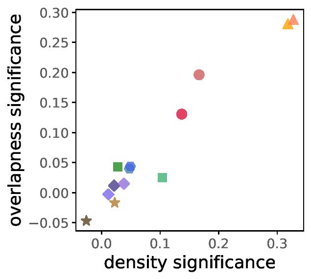
Figure 1. Hypergraphs from the same domain share similar hyperedge overlapping patterns at the egonet level.

4.2. L2. Pair/Triple of Nodes Level

Given a pair or triple of nodes, how many hyperedges do overlap at them? In other words, how many hyperedges do contain the pair or triple? While the degree is generally defined as the number of hyperedges that contains each individual node, here we extend the concept to pairs and triples of nodes. Specifically, if we let $E_{S}:=\{e\in E:S\subseteq e\}$ be the set of hyperedges overlapping at a subset $S\subseteq V$ of nodes, then the degree of each node pair $\{i,j\}$ is defined as $d^{(2)}(\{i,j\}):=|E_{\{i,j\}}|$, and the degree of each node triple $\{i,j,k\}$ is defined as $d^{(3)}(\{i,j,k\}):=|E_{\{i,j,k\}}|$. The degree of a pair or triple can also be interpreted as the structural similarity between the nodes in the pair or triple. Intuitively, nodes are structurally more similar as they are included together in more hyperedges.

Examining the degree distributions of pairs and triples of nodes, instead of that of individual nodes, gives higher-order insights on how nodes as a set form hyperedges. In the third and fourth columns of Table 4, we provide the distributions of $d^{(2)}$ and $d^{(3)}$ in real-world hypergraphs and those in a corresponding randomized hypergraph. Our findings are summarized in Observations 3 and 4.

Observation 3.

The number of hyperedges overlapping at each pair of nodes (i.e., degree of each pair) is more skewed with a heavier tail in real-world hypergraphs than in randomized ones. The distribution is similar to a truncated power law distribution.

Observation 4.

The number of hyperedges overlapping at each triple of nodes (i.e., degree of each triple) is more skewed with a heavier tail in real-world hypergraphs than in randomized ones. The distribution is similar to a truncated power law distribution.

Table 6. The distribution of the number of hyperedges overlapping at each pair or triple of nodes is heavy-tailed and close to a truncated power-law distribution. This claim is supported by the reported log-likelihood ratios when fitting the distributions to each of three heavy-tailed distributions (power-law, truncated power-law, and log normal) against the exponential distribution.

Dataset	Pair of Nodes (Obs. 3)				Triple of Nodes (Obs. 4)
	pw	tpw	logn		pw	tpw	logn
email-Enron	-0.36	4.22	3.50		1.91	3.88	3.47
email-Eu	0.66	1.48	1.29		0.21	0.77	0.63
contact-primary	0.64	1.40	1.35		0.01	0.48	0.48
contact-high	0.75	0.81	0.79		-1.04	-	0.80
NDC-classes	13.49	15.74	14.78		24.37	31.53	29.19
NDC-substances	38.68	43.87	42.55		102.90	116.45	109.77
tags-ubuntu	39.66	41.55	41.25		17.03	17.84	17.79
tags-math	3.82	4.49	4.47		26.97	29.26	29.07
threads-ubuntu	3.79	3.97	3.97		0.34	0.80	0.73
threads-math	14.25	14.78	14.68		-1.04	-0.09	-1.12
coauth-DBLP	19.23	22.47	22.31		5.75	5.84	5.83
coauth-geology	45.20	53.39	52.92		9.69	13.73	13.01
coauth-history	3.74	3.81	3.91		-0.36	1.42	1.27

In addition to the visual inspection, we compute the log-likelihood ratio of three representative heavy-tailed distributions (power-law, truncated power-law, and log normal) against the exponential distribution, as suggested in (Alstott et al., 2014; Clauset et al., 2009). If the ratio is greater than $0$, the given distribution is more similar to the corresponding heavy-tailed distribution than an exponential distribution. As reported in Table 6, except for one case, at least one heavy-tailed distribution has a positive ratio, and in most cases the ratio is highest for truncated power-law distributions. These result support the claim that the degree distributions of pairs and triples of nodes is heavy-tailed and similar to truncated power-law distributions.

In fact, these results are intuitive. The more often a pair or triple of nodes interact together, the more likely they are to interact together again. For example, researchers that have co-authored multiple papers are likely to share common interests, which can lead to more collaborations in the future.

Table 7. The distributions of hyperedge homogeneity in real hypergrpahs and those generated by are heavy-tailed. Log-likelihood ratios are calculated as in Table 6.

Dataset	Real-World Data				Generated
	pw	tpw	logn		pw	tpw	logn
email-Enron	-1.09	-0.26	-0.38		-2.71	-0.43	-4.76
email-Eu	0.90	0.90	0.91		-3.00	3.13	2.08
contact-primary	2.19	2.30	2.22		0.67	2.26	1.90
contact-high	1.55	1.55	1.95		2.50	4.72	3.65
NDC-classes	0.00	0.39	0.18		-0.47	0.87	0.52
NDC-substances	0.64	1.22	1.13		1.87	2.90	2.58
tags-ubuntu	2.25	2.25	2.26		-2.01	7.00	6.19
tags-math	-17.66	-7.93	2.62		3.53	6.56	6.07
threads-ubuntu	4.58	7.70	6.55		3.92	4.25	3.94
threads-math	-0.72	9.00	6.69		4.30	12.10	10.53
coauth-DBLP	4.01	4.31	4.20		10.65	25.23	22.82
coauth-geology	4.29	5.52	5.37		1.75	8.06	7.00
coauth-history	-	-	1.73		3.98	4.31	4.02

4.3. L3. Hyperedge Level

How are nodes that form hyperedges together related to each other? It is unlikely in real-world hypergraphs that each hyperedge is formed by nodes chosen independently at random. It is expected to exist a strong dependency among the nodes forming a hyperedge together. In order to investigate the dependency, we use the homogeneity of hyperedge, defined in Definition 3, to measure how structurally similar such nodes are.

Definition 3 (Homogeneity of a Hyperedge).

The homogeneity of a hyperedge $e\in E$ is defined as follow:

(1) $$homogeneity(e):=\begin{cases}\frac{\sum_{\{u,v\}\in\binom{e}{2}}|E_{\{u,v\}}|}{\binom{|e|}{2}},&\mathrm{if}\ |e|>1\\ 0,&\mathrm{otherwise,}\end{cases}$$

where $\binom{e}{2}$ is the set of node pairs in $e$ and $|E_{\{u,v\}}|$ is the number of hyperedges overlapping at the pair of $u$ and $v$ (i.e., the degree of the pair $\{u,v\}$). Note that, in Eq. (1), the structural similarity between two nodes is measured in terms of the number of hyperedges overlapping at them, which we examine in Section 4.2. Eq. (1) can be easily extended to three or more nodes.

The figures in the last row of Table 4 show the homogeneity of the hyperedges in real-world hypergraphs and corresponding randomized hypergraphs. As summarized in Observation 5, there is a tendency that the homogeneity of each hyperedge in real-world hypergraphs is greater than that in randomized ones. Moreover, we verify that the distribution of homogeneity is heavy-tailed (see Table 7), as in the previous subsection.

Observation 5.

Hyperedges in real-world hypergraphs tend to contain structurally more similar nodes (i.e., nodes where many hyperedges overlap) than those in randomized hypergraphs.

The homogeneity of hyperedges plays a key role in generating realistic hypergraphs, as described in the following section.

5. Hypergraph Generation

We have shown that overlapping patterns of hyperedges in real-world hypergraphs are clearly distinguished from those in randomized hypergraphs. In this section, we propose , a scalable and realistic hypergraph generative model that reproduces the realistic overlapping patterns of hyperedges. After describing , we present , which automatically tunes the parameters of so that hypergraphs similar to a given target hypergraph are generated. Then, we evaluate and experimentally.

5.1. : Multilevel HyperCL 

We propose , a realistic hypergraph generative model whose pseudocode is described in Algorithm 2. The key idea behind is to extend HyperCL to multiple levels. Recall that HyperCL itself cannot accurately reproduce realistic overlapping patterns, as shown in Section 4.

Input :  (1) distribution of hyperedge sizes $\{s_{1},\cdots,s_{|E|}\}$

(2) distribution of node degrees $\{d_{1},\cdots,d_{|V|}\}$

(3) number of levels $L$ ($\leq\log_{2}|V|$)

(4) weights of each level $\{w_{1},\cdots,w_{L}\}$

Output :  synthetic hypergraph $\hat{G}=(\hat{V},\hat{E})$

1

2/* Initialization */

3 $\hat{V}\leftarrow\{1,\cdots,|V|\}$ and $\hat{E}\leftarrow\varnothing$

4

5/* Hierarchical Node Partitioning */ 

6 $S_{1}^{(L)},\cdots,S_{2^{L-1}}^{(L)}\leftarrow$ uniformly partition $\hat{V}$ into $2^{L-1}$ groups

7 for each level $\ell=L-1,\cdots,1$ do

8       for each group $\textsl{g}=1,\cdots,2^{\ell-1}$ do

9             $S_{g}^{(\ell)}=S_{2g-1}^{(\ell+1)}\cup S_{2g}^{(\ell+1)}$

10            

11      

12

13/* Hyperedge Generation */

14 for each $i=1,\cdots,|E|$ do

15       $\ell\leftarrow$ select a level with prob. proportional to the weight

16       $S_{g}^{(\ell)}\leftarrow$ select a group at level $\ell$ uniformly at random

17       $\hat{e_{i}}\leftarrow\varnothing$

18       while $|\hat{e_{i}}|<s_{i}$ do

19             $v\leftarrow$ select a node from $S_{g}^{(\ell)}$ with prob. proportional to the degree

20             $\hat{e_{i}}=\hat{e_{i}}\cup\{v\}$

21            

22      $\hat{E}=\hat{E}\cup\{\hat{e_{i}}\}$

23      

24

return $\hat{G}=(\hat{V},\hat{E})$

Algorithm 2 : Realistic Hypergraph Generator

Description of : , a multilevel extension of HyperCL, requires two additional inputs: (1) number of levels $L$ and (2) weights of each level $\{w_{1},\cdots,w_{L}\}$. For now, we assume that the parameters are given; how to set the parameters is discussed in the next subsection. consists of the hierarchical node partitioning step and the hyperedge generation step.

Step 1. Hierarchical Node Partitioning (lines 2 - 2). first partitions nodes into groups at every level. Specifically, at every level $\ell\in\{1,\cdots,L\}$, it randomly divides nodes $2^{\ell-1}$ groups, denoted by $S_{1}^{(\ell)},\cdots,S_{2^{\ell-1}}^{(\ell)}$ while satisfying the following conditions:

1. $S_{i}^{(\ell)}\cap S_{j}^{(\ell)}=\varnothing$ for all $i\neq j\in\{1,\cdots,2^{\ell-1}\}$,

2. $|\bigcup_{i=1}^{2^{\ell-1}}S_{i}^{(\ell)}|=|V|$,

3. $|S_{i}^{(\ell)}|=\lfloor\frac{|V|\cdot i}{2^{\ell-1}}\rfloor-\lfloor\frac{|V|\cdot(i-1)}{2^{\ell-1}}\rfloor$ for all $i\in\{1,\cdots,2^{\ell-1}\}$,

4. $S_{i}^{(\ell)}=S_{2i-1}^{(\ell+1)}\cup S_{2i}^{(\ell+1)}$ for all $\ell<L$, and $i\in\{1,\cdots,2^{\ell-1}\}$.

The first and second conditions ensure that at each level each node belongs to exactly one group. The third condition states that the size of groups at each level are almost uniform. The last condition states that the groups are hierarchical. That is, if nodes are in the same group at a level, then they are in the same group at all lower levels. Note that nodes are divided more finely into smaller subsets at higher levels. At the lowest level $1$, there exist a single group, which is the same as the entire set of nodes $V$, whereas at the highest level $L$, there exist most groups whose number is $2^{L-1}$.

Step 2. Hyperedge Generation (lines 2 - 2). Once we partition nodes hierarchically in the previous step, for each $i$-th hyperedge $\hat{e_{i}}$, first selects a level with probability proportional to the weight of each level. That is, each level $\ell$ is selected with probability proportional to $w_{\ell}$. At the selected level $\ell$, selects a group $S_{g}^{(\ell)}$ uniformly at random. Then, the nodes forming $\hat{e_{i}}$ are sampled independently, with probability proportional to the degree of each node, until the size of the hyperedge reaches $s_{i}$. That is, instead of taking all nodes into consideration, we divide the nodes into multiple groups and limit the nodes that a hyperedge can contain into those in a group. Note that hyperedges generated within the same group at higher levels are more likely to be overlapped each other, as fewer nodes are in each group at a higher level. Practically, since $\hat{e_{i}}$ cannot be generated from a group whose size is smaller than $s_{i}$, we select level $\ell$ such that $\ell\leq\log_{2}{\frac{|V|}{s_{i}}}+1$.

Degree Preservation of : In hypergraphs generated by , the size distribution of hyperedges is exactly the same as the input size distribution. Specifically, $|\hat{e_{i}}|=s_{i}$ holds for all $i\in\{1,\cdots,|E|\}$. The degree distribution of nodes is also expected to be similar to the input degree distribution. In order to show this, we first provide Lemma 1, which our analysis is based on.

Lemma 1.

For each group $S_{g}^{(\ell)}$ at level $\ell$, the probability for a hyperedge $e$ to be generated from $S_{g}^{(\ell)}$ is

(2) $$~{}P[e\subseteq S_{g}^{(\ell)}]=\frac{w_{\ell}}{W_{e}}\cdot\frac{1}{2^{\ell-1}},$$

where $W_{e}$ is the sum of the weights of suitable levels. That is, $W_{e}=\sum_{k=1}^{L_{e}}w_{k}$ where $L_{e}=\lfloor\log_{2}{\frac{|V|}{s_{i}}+1}\rfloor$.

Proof. Given any hyperedge $e$, first randomly selects a suitable level with probability proportional to the given weight. Thus, the probability for the level $\ell$ to be selected is $w_{\ell}/W_{e}$. Once the level is determined, any of the $2^{\ell-1}$ groups in level $\ell$ is selected uniformly at random, i.e., with probability $1/2^{\ell-1}$. The probability for $e$ to be generated from $S_{g}^{(\ell)}$ is the product of the two probabilities, and thus Eq. (2) holds. $\blacksquare$

For each node $v$, let $\hat{d}_{v}^{(\ell)}$ be the number of hyperedges that contain the node $v$ among those generated at level $\ell$. Then, the degree $\hat{d}_{v}$ of $v$ in an output hypergraph is the sum of $\hat{d}_{v}^{(\ell)}$ over all levels, i.e., $\hat{d}_{v}=\sum_{\ell=1}^{L}\hat{d}_{v}^{(\ell)}$. Let $d_{max}:=\max_{k\in\{1,\cdots,|V|\}}d_{k}$ and $s_{max}=\max_{k\in\{1,\cdots,|E|\}}s_{k}$. Assume $|V|\gg 2^{L-1}\cdot d_{max}$ and $\sum_{j\in S_{g}^{(\ell)}}d_{j}\gg d_{max}\cdot s_{max}$ for all $S_{g}^{(\ell)}$. Then,

$$\mathbb{E}[\hat{d}_{v}] =\sum_{\ell=1}^{L}\mathbb{E}[\hat{d}_{v}^{(\ell)}]=\sum_{\ell=1}^{L}\sum_{e\in E}P[e\subseteq S_{g}^{(\ell)}(v)]\cdot P[v\in e|e\subseteq S_{g}^{(\ell)}(v)]$$

$$\approx\sum_{e\in E}\sum_{\ell=1}^{L_{e}}\left(\frac{w_{\ell}}{W_{e}}\cdot\frac{1}{2^{\ell-1}}\right)\left[|e|\cdot\left(\frac{d_{v}\cdot 2^{\ell-1}}{\sum_{j=1}^{|V|}d_{j}}\right)\right]$$

$$=\frac{d_{v}}{\sum_{j=1}^{|V|}d_{j}}\cdot\sum_{e\in E}\left(|e|\cdot\sum_{\ell=1}^{L_{e}}\frac{w_{\ell}}{W_{e}}\right)={\color[rgb]{0,0,0}d_{v}\cdot\frac{\sum_{e\in E}|e|}{\sum_{j=1}^{|V|}d_{j}}}=d_{v},$$

where $S_{g}^{(\ell)}(v)$ is the group at level $\ell$ containing $v$. That is, $\hat{d}_{v}$ is expected to be close to $d_{v}$, as we confirm empirically in (onl, 2021).

1

Input : (1) input hypergraph $G=(V,E)$

(2) update resolution $p$

Output : synthetic hypergraph $\hat{G}=(\hat{V},\hat{E})$

2 $\hat{G}=(\hat{V},\hat{E})\leftarrow$ run HyperCL using the distributions in $G$

3 for each level $\ell=2,\cdots,L$ do

4       $i^{*}\leftarrow\operatorname*{arg\,min}_{i\in\{1,\cdots,1/p\}}HHD\left(G,\mathtt{update}(\hat{G},p\cdot i,\ell)\right)$

5       $\bar{G}\leftarrow\mathtt{update}(\hat{G},p\cdot i^{*},\ell)$

6       if $HHD(G,\bar{G})<HHD(G,\hat{G})$ then  $\hat{G}\leftarrow\bar{G}$

7       else  break

8      

9return $\hat{G}=(\hat{V},\hat{E})$

1 update($\hat{G}=(\hat{V},\hat{E})$, $q$, $\ell$)

2       $\bar{G}(\bar{V},\bar{E})\leftarrow\hat{G}(\hat{V},\hat{E})$

3       remove $(q\cdot 100)\%$ of the hyperedges created at level $\ell-1$

4       create the same number of hyperedges at level $\ell$

5       return $\bar{G}=(\bar{V},\bar{E})$

Algorithm 3 : Automatic Parameter Selection

Table 8. D-statistics between the distributions of (1) egonet density, (2) egonet overlapness and (3) hyperedge homogeneity in real-world hypergraphs and corresponding hypergraphs generated by five models: HyperCL (H-CL), HyperPA (H-PA), HyperFF (H-FF), (H-LAP), and (H-LAP⁺). reproduces the distributions most accurately.

Dataset	Density of Egonets (Obs. 1)						Overlapness of Egonets (Obs. 2)						Homogeneity of Hyperedges (Obs. 5)
	H-CL	H-PA	H-FF	H-LAP	H-LAP+		H-CL	H-PA	H-FF	H-LAP	H-LAP+		H-CL	H-PA	H-FF	H-LAP	H-LAP+
email-Enron	0.545	0.202	0.391	0.405	0.125		0.517	0.398	0.398	0.391	0.111		0.498	0.241	0.656	0.191	0.136
email-Eu	0.724	-	0.402	0.577	0.310		0.534	-	0.639	0.432	0.197		0.505	-	0.688	0.247	0.168
contact-primary	0.896	0.537	0.975	0.334	0.128		0.867	0.471	0.942	0.285	0.095		0.430	0.236	0.484	0.142	0.188
contact-high	0.948	0.529	0.880	0.522	0.345		0.874	0.431	0.703	0.486	0.296		0.423	0.196	0.336	0.120	0.178
NDC-classes	0.694	0.785	0.731	0.696	0.635		0.302	0.715	0.406	0.231	0.248		0.274	0.410	0.484	0.272	0.225
NDC-substances	0.451	-	0.801	0.426	0.366		0.321	-	0.338	0.243	0.157		0.377	-	0.740	0.262	0.108
tags-ubuntu	0.522	0.162	0.216	0.410	0.300		0.432	0.117	0.398	0.487	0.210		0.245	0.136	0.844	0.105	0.011
tags-math	0.496	0.350	0.561	0.195	0.227		0.460	0.325	0.709	0.151	0.186		0.337	0.217	0.921	0.086	0.015
threads-ubuntu	0.159	0.856	-	0.163	0.159		0.299	0.953	-	0.300	0.297		0.020	0.291	-	0.016	0.011
threads-math	0.137	0.492	-	0.120	0.135		0.232	0.714	-	0.235	0.229		0.060	0.368	-	0.102	0.019
coauth-DBLP	0.228	-	-	0.227	0.132		0.302	-	-	0.267	0.244		0.715	-	-	0.540	0.026
coauth-geology	0.200	-	-	0.202	0.138		0.248	-	-	0.252	0.266		0.624	-	-	0.481	0.044
coauth-history	0.087	-	-	0.090	0.089		0.316	-	-	0.321	0.324		0.154	-	-	0.125	0.020
Average	0.468	0.489	0.619	0.335	0.237		0.439	0.515	0.566	0.313	0.219		0.358	0.261	0.644	0.206	0.088
-: out of time (taking more than 10 hours) or out of memory

Table 9. Distributions of the number of overlapping hyperedges at each pair and each triple of nodes are reproduced accurately by , while HyperCL fails in many cases. They obey heavy-tailed distribution, as in the real ones.

	email-Eu	contact-primary	NDC-substances	tags-math	threads-ubuntu	coauth-DBLP
Observation 3
Observation 4

Intuition Behind : In this section, we provide some reasons why we expect to accurately reproduce the realistic overlapping patterns of hyperedges discovered in Section 4.

• For a pair or triple of nodes belonging to the same small group, the number of hyperedges overlapping at them is expected to be high. Thus, the distribution of the number of overlapping hyperedges at each pair or triple is expected to be skewed.

• As hyperedges can be formed within a small group, which contains structurally similar nodes, the homogeneity of each hyperedge is expected to be high. Moreover, as the size of groups varies, the homogeneity of hyperedges is expected to vary depending on the size of the groups that they are generated from.

• As the hyperedges in the egonet of each node $v$ are likely to contain nodes belonging to the same small group with $v$, their density and overlapness are expected to be high.  
  

5.2. : Parameter Selection

Given an input hypergraph $G$, how can we set the parameters of (i.e., the number of levels $L$ and the weight of each level $\{w_{1},\cdots,w_{L}\}$) so that it generates a synthetic hypergraph $\hat{G}$ especially similar to a target real-world hypergraph? The parameters should be carefully tuned since the structural properties of the generated hypergraphs vary depending on their settings. To this end, we propose , which automatically tunes the parameters.

Hyperedge Homogeneity Objective: As its objective function, uses the hyperedge homogeneity distance $HHD(G,\hat{G})$ between the input hypergraph $G$ and a generated hypergraph $\hat{G}$. It is defined as the Kolmogorov-Smirnov D-statistics between the hyperedge homogeneity distribution of $G$ and that of $\hat{G}$. That is,

(3) $$HHD(G,\hat{G})=\max_{x}\{|F(x)-F^{\prime}(x)|\},$$

where $F$ and $F^{\prime}$ are the cumulative hyperedge homogeneity distribution of hypergraph $G$ and $\hat{G}$, respectively. Then, assuming that the number of levels $L$ is given, aims to find the weights of levels that minimize the hyperedge homogeneity distance. That is, aims to solve the following optimization problem:

$$\min_{w_{1},\cdots,w_{L}}HHD(G,\hat{G}),$$

where we assume $w_{1}+\cdots+w_{L}=1$ since only the ratios between the weights matter.

Table 10. D-statistics between the distributions of the number of overlapping hyperedges at each pair and each triple of nodes in real-world hypergraphs and corresponding hypergraphs generated by five models: HyperCL (H-CL), HyperPA (H-PA), HyperFF (H-FF), (H-LAP), and (H-LAP⁺). reproduces the distributions most accurately, and these distributions follow heavy-tailed distributions.

Dataset	Pair of Nodes (Obs. 3)										Triple of Nodes (Obs. 4)
	Distance from Real (D-statistics)						Heavy-tail Test				Distance from Real (D-statistics)						Heavy-tail Test
	H-CL	H-PA	H-FF	H-LAP	H-LAP+		pw	tpw	logn		H-CL	H-PA	H-FF	H-LAP	H-LAP+		pw	twp	logn
email-Enron	0.143	0.056	0.217	0.075	0.139		-2.37	-0.29	-1.53		0.089	0.295	0.136	0.061	0.072		-0.22	0.38	0.24
email-Eu	0.225	-	0.352	0.162	0.066		0.24	2.75	2.53		0.480	-	0.516	0.337	0.206		0.41	2.11	1.96
contact-primary	0.196	0.062	0.223	0.070	0.051		9.53	15.74	13.92		0.137	0.061	0.110	0.053	0.031		-1.86	-1.27	1.23
contact-high	0.277	0.062	0.141	0.127	0.067		-3.09	-0.95	-0.06		0.210	0.131	0.182	0.182	0.193		-3.95	-	0.50
NDC-classes	0.273	0.197	0.196	0.246	0.172		12.15	14.42	14.04		0.376	0.167	0.405	0.349	0.286		3.22	7.92	7.34
NDC-substances	0.272	-	0.244	0.251	0.202		33.69	40.13	39.66		0.521	-	0.591	0.492	0.453		45.30	55.38	54.99
tags-ubuntu	0.091	0.019	0.182	0.034	0.033		42.33	43.70	43.55		0.148	0.067	0.191	0.020	0.074		14.25	15.57	15.43
tags-math	0.095	0.066	0.278	0.073	0.011		42.75	45.60	45.41		0.209	0.053	0.286	0.113	0.079		21.38	23.12	22.99
threads-ubuntu	0.011	0.137	-	0.008	0.009		1.28	1.75	1.75		0.004	0.130	-	0.004	0.004		-1,346	-1.72	-1.72
threads-math	0.041	0.163	-	0.014	0.033		15.79	16.66	16.52		0.006	0.138	-	0.001	0.005		-1.49	-0.98	0.96
coauth-DBLP	0.224	-	-	0.191	0.032		55.86	74.95	73.45		0.215	-	-	0.214	0.192		2.87	6.73	6.46
coauth-geology	0.178	-	-	0.157	0.040		31.13	45.08	44.06		0.086	-	-	0.085	0.069		-0.10	1.10	0.84
coauth-history	0.033	-	-	0.030	0.009		1.74	1.77	1.63		0.001	-	-	0.001	0.001		-0.86	-	0.57
Average	0.158	0.095	0.229	0.110	0.066						0.193	0.130	0.302	0.147	0.128
-: out of time (taking more than 10 hours) or out of memory

Optimization Scheme: Having defined the objective, we describe how minimizes it. To avoid empty groups, $L\leq\log_{2}|V|$ should hold, and the number of levels $L$ is initialized to $\lfloor\log_{2}|V|\rfloor$.

Since there are infinitely many combinations of level weights $w_{1},\cdots,w_{L}$, we propose an efficient greedy optimization scheme described in Algorithm 3, where some fraction of hyperedges created at a lower level are replaced with those newly created at a higher level, repeatedly, until Eq. (3) converges.

Specifically, first generates a hypergraph by HyperCL, which is equivalent to with $L=1$ (line 3). This is equivalent to set $w_{1}$ to $1$ and set $w_{\ell}$ to $0$ for all $\ell>1$. Then at each level $\ell$ from $2$ to $L$, we search for an optimal fraction of hyperedges created at level $\ell-1$ to be replaced with those newly created at level $\ell$ (line 3). Note that only hyperedges of size $\frac{|V|}{2^{\ell-1}}$ or smaller can be replaced. If the replacement strictly decreases the hyperedge homogeneity distance, then updates the current synthetic hypergraph (line 3). This is equivalent to decrease $w_{\ell-1}$ and increase $w_{\ell}$ by the same amount. Otherwise, we return the current synthetic hypergraph (line 3). We fix the update resolution $p$ to $0.05$ throughout this work. We note that the quality of generated hypergraphs is empirically insensitive to the choices of $p$.

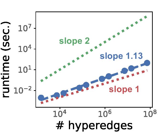
(a) (generation)

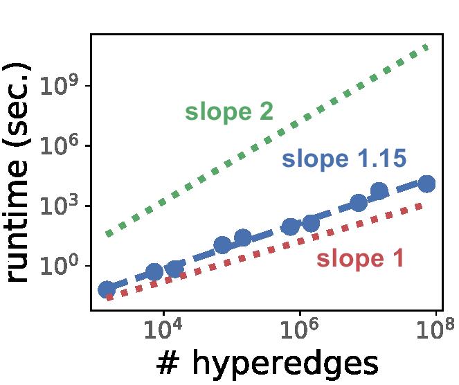
(b) (generation & fitting)

Figure 2. and scale near linearly with the size of the considered hypergraph. 

5.3. Empirical Evaluation of the Quality of Generated Hypergraphs

How well do the hypergraphs generated by reproduce the structural properties of the input hypergraphs? We evaluate its effectiveness by comparing them with four strong baselines: HyperCL, HyperPA (Do et al., 2020), HyperFF (Kook et al., 2020), and naïvely tuned . We describe the detailed experimental settings at Appendix B.

To measure the similarity between the distributions derived from the real-world hypergraph and the generated hypergraph, we use the Kolmogorov-Smirnov D-statistic, defined as $D=\max_{x}\{|F^{\prime}(x)-F(x)|\}$, where $x$ is a value of the considered random variable, and $F^{\prime}$ and $F$ are the cumulative distribution functions of the real and corresponding generated distributions.

Observations 1 and  2: In Table 8, we report the D-statistics between the distributions of egonet density and egonet overlapness in real-world hypergraphs and corresponding synthetic hypergraphs. generates hypergraphs that consist of egonets that are structurally most similar to those in real-world hypergraphs. Specifically, gave $\mathbf{2.06\times}$ more similar egonet density distribution and $\mathbf{2.35\times}$ more similar egonet overlapness distribution than recently proposed HyperPA.

Observations 3 and  4: We visually and statistically test whether the hypergraphs generated by follow observations 3 and 4. In Table 9, we illustrate the distributions of the number of hyperedges overlapping at each pair and each triple of nodes. Compared to HyperCL, better reproduces the degrees of pairs and triples of nodes. This is statistically confirmed in Table 10, where gives the smallest D-statistic. In addition, these distributions are heavy-tailed in most datasets, as seen from the fact that at least one likelihood ratio is positive (see Section 4.2 for the details of the statistical test).

Observation 5: From the results in Table 8, we can see that the D-statistics between the distributions of hyperedge homogeneity in real-world and corresponding hypergraphs generated by are extremely small. Since the objective of is to reduce the $HHD$, it naturally reproduce hyperedge homogeneity better than HyperCL, which surprisingly outperforms when its parameters are naïvely set. This result suggests the effectiveness of the proposed optimization scheme. As seen in Table 7, the distributions of hyperedge homogeneity in hypergraphs generated by are heavy-tailed (see Section 4.2 for the details of the statistical test).

5.4. Scalability of and

In this subsection, we analyze the scalability of and both theoretically and experimentally. Noteworthy, we show empirically that both and scale almost linearly with the size of the considered hypergraph.

In fact, while some baselines are intractable in particular datasets, and are scalable enough to be executed in all considered datasets. The scalability of HyperPA heavily depends on the sizes of hyperedges, and thus does not work in hypergraphs that includes large-sized hyperedges (i.e., email-Eu, NDC-substances, coauth-DBLP, coauth-geology, and coauth-history). HyperFF depends on the number of nodes, and does not work in large datasets with many nodes (i.e., threads-ubuntu, threads-math, coauth-DBLP, coauth-geology, and coauth-history).

Given the number of levels and weights of each level, how much time does it take to run ? Assume that all sets and maps are implemented using hash tables. For each hyperedge $e$, level $\ell$ and group $g$ are selected in $O(1)$ time. In addition, since each node is sampled independently, $|e|$ nodes are selected in $O(|e|\cdot(1+\epsilon))$ time, where $\epsilon$ is due to the possibility of collisions (i.e., nodes selected multiple times for a hyperedge). The term $\epsilon$ depends on the degrees of nodes and the sizes of hyperedges. We note that $\epsilon$ is empirically very small in the considered datasets. Hence, generating $|E|$ hyperedges takes $O(\sum_{e\in E}(|e|\cdot(1+\epsilon)))$ time. In , we consider the replacement step. At each level, at most $\frac{1}{p}\cdot|E|=O(|E|)$ hyperedges are (temporarily) replaced, taking $O(\sum_{e\in E}(|e|\cdot(1+\epsilon)))$ time. Since the maximum number of levels is $\log_{2}|V|$, takes $O(\log_{2}|V|\cdot\sum_{e\in E}(|e|\cdot(1+\epsilon)))$ time in total.

In Figure 2, we measure the runtimes of and with synthetic hypergraphs of different sizes. They are generated by upscaling the smallest hypergraph, email-Enron by $5$ to $50,000$ times, using . Both and scale almost linearly with the size of the considered hypergraph. Specifically, generates and fits a synthetic hypergraph with 0.7 billion hyperedges within few hours. We describe the detailed experimental settings at Appendix B.

6. Conclusions

In this work, we investigate the structural properties regarding the overlaps of hyperedges of thirteen real-world hypergraphs from six domains. To this end, we define several principled measures, and based on the observations, we develop a realistic hypergraph generative model. We summarize our contributions as follows.

• Observations in Real-world Hypergraphs: We discover three unique properties of the overlaps of hyperedges in real-world hypergraphs. We verify these properties using randomized hypergraphs where both the degrees of nodes and the sizes of hyperedges are well preserved.

• Novel Measures: We propose the overlapness and homogeneity of hyperedges. We demonstrate through an axiomatic approach that overlapness is a principled measure. Homogeneity reveals an interesting overlapping pattern, based on which we develop a realistic generative model.

• Realistic Generative Model: We propose , a hypergraph generative model that accurately reproduces the overlapping patterns of hyperedges in real-world hypergraphs. We also provide , which automatically fits the parameters of to a given graph. They generate and fit a hypergraph with $0.7$ billion hyperedges within few hours.

Reproducibility: The source code and datasets used in this work are available at https://github.com/young917/www21-hyperlap.

Acknowledgements We thank Dr. Jisu Kim for fruitful discussions. This work was supported by National Research Foundation of Korea (NRF) grant funded by the Korea government (MSIT) (No. NRF-2020R1C1C1008296) and Institute of Information & Communications Technology Planning & Evaluation (IITP) grant funded by the Korea government (MSIT) (No. 2019-0-00075, Artificial Intelligence Graduate School Program (KAIST)).

Appendix A Appendix: Axioms of Overlapness 

We systematically analyze overlapness defined in Section 4.1 by comparing with possible baselines and proving that the metric satisfies all the proposed axioms.

Baselines: Due to the simplicity and intuitiveness of the aforementioned axioms, one might hypothesize that it is trivial to satisfy them. However, as seen in Table 5, none of the other possible baseline metrics obey all three axioms. We consider five different baseline metrics including two basic set operations:

• Intersection: $|\bigcap_{e\in\mathcal{E}}e|$

• Union Inverse: $1/|\bigcup_{e\in\mathcal{E}}e|$

• Jaccard Index: $|\bigcap_{e\in\mathcal{E}}e|/|\bigcup_{e\in\mathcal{E}}e|$

• Overlap Coefficient: $|\bigcap_{e\in\mathcal{E}}e|/\min_{e\in\mathcal{E}}|e|$

• Density (Hu et al., 2017): $|\mathcal{E}|/|\bigcup_{e\in\mathcal{E}}e|$

Using the intersection of multiple hyperedges as the measure is applicable to only a small number of hyperedges (i.e., small $k$) due to its strict condition that nodes should be included in all the given hyperedges. Accordingly, other possible measures to gauge the overlaps such as the Jaccard index or the overlap coefficient, which use intersection size as a numerator, face the same challenge. The inverse of the union meets Axiom 2, while it does not satisfy Axiom 1 and Axiom 3. The density of the hyperedges satisfies Axiom 1 and Axiom 2, while it does not satisfy Axiom 3, which is clear from the example discussed in Section 4.1. We provide detailed examples and reasons why each baseline measure does not satisfy at least one axiom in the online appendix (onl, 2021).

Proof of Theorem 1: We show that overlapness meets all three axioms discussed in Section 4.1. That is, we prove Theorem 1 by proving Lemmas 2, 3, and 4, which Theorem 1 follows from.

Lemma 2.

Overlapness meets Axiom 1.

Proof. Considering the conditions in Axiom 1, we compare the overlapness of $\mathcal{E}$ and $\mathcal{E}^{\prime}$:

$$o(\mathcal{E}^{\prime})-o(\mathcal{E})=\frac{\sum_{e^{\prime}\in\mathcal{E}^{\prime}}|e^{\prime}|}{|\bigcup\nolimits_{e^{\prime}\in\mathcal{E}^{\prime}}e^{\prime}|}-\frac{\sum_{e\in\mathcal{E}}|e|}{|\bigcup\nolimits_{e\in\mathcal{E}}e|}=\frac{n\cdot(|\mathcal{E}^{\prime}|-|\mathcal{E}|)}{|\bigcup\nolimits_{e\in\mathcal{E}}e|}$$

from the conditions $|\bigcup\nolimits_{e\in\mathcal{E}}e|=|\bigcup\nolimits_{e^{\prime}\in\mathcal{E}^{\prime}}e^{\prime}|$ and $|e|=|e^{\prime}|=n,\ \forall e\in\mathcal{E},\ \forall e^{\prime}\in\mathcal{E}^{\prime}$. Since the number of hyperedges in $\mathcal{E}^{\prime}$ is larger than that in $\mathcal{E}$ (i.e., $|\mathcal{E}^{\prime}|>|\mathcal{E}|$), $o(\mathcal{E}^{\prime})>o(\mathcal{E})$ holds. This implies Axiom 1. $\blacksquare$

Lemma 3.

Overlapness meets Axiom 2.

Proof. Considering the conditions in Axiom 2, we compare the overlapness of $\mathcal{E}$ and $\mathcal{E}^{\prime}$:

$$\frac{o(\mathcal{E}^{\prime})}{o(\mathcal{E})}=\frac{\sum_{e^{\prime}\in\mathcal{E}^{\prime}}|e^{\prime}|}{|\bigcup\nolimits_{e^{\prime}\in\mathcal{E}^{\prime}}e^{\prime}|}\bigg{/}\frac{\sum_{e\in\mathcal{E}}|e|}{|\bigcup\nolimits_{e\in\mathcal{E}}e|}=\frac{|\bigcup\nolimits_{e\in\mathcal{E}}e|}{|\bigcup\nolimits_{e^{\prime}\in\mathcal{E}^{\prime}}e^{\prime}|}$$

from the conditions $|\mathcal{E}|=|\mathcal{E^{\prime}}|=n$ and $|e_{i}|=|e^{\prime}_{i}|,\ \forall i\in\{1,...,n\}$. Since the number of nodes in $\mathcal{E}$ is more than $\mathcal{E}^{\prime}$ (i.e., $|\bigcup\nolimits_{e\in\mathcal{E}}e|>|\bigcup\nolimits_{e^{\prime}\in\mathcal{E}^{\prime}}e^{\prime}|$, $\frac{o(\mathcal{E}^{\prime})}{o(\mathcal{E})}>1$ holds, and thus $o(\mathcal{E}^{\prime})>o(\mathcal{E})$. This implies Axiom 2. $\blacksquare$

Lemma 4.

Overlapness meets Axiom 3.

Proof. Considering the conditions in Axiom 3, we compare the overlapness of $\mathcal{E}$ and $\mathcal{E}^{\prime}$:

$$o(\mathcal{E}^{\prime})-o(\mathcal{E})=\frac{\sum_{e^{\prime}\in\mathcal{E}^{\prime}}|e^{\prime}|}{|\bigcup\nolimits_{e^{\prime}\in\mathcal{E}^{\prime}}e^{\prime}|}-\frac{\sum_{e\in\mathcal{E}}|e|}{|\bigcup\nolimits_{e\in\mathcal{E}}e|}=\frac{\sum\nolimits_{k=1}^{n}(|e^{\prime}_{k}|-|e_{k}|)}{|\bigcup\nolimits_{e\in\mathcal{E}}e|}$$

from the conditions $|\mathcal{E}|=|\mathcal{E}^{\prime}|=n$ and $|\bigcup\nolimits_{e\in\mathcal{E}}e|=|\bigcup\nolimits_{e^{\prime}\in\mathcal{E}^{\prime}}e^{\prime}|$. Since $|e_{i}|<|e^{\prime}_{i}|$, and $|e_{j}|\leq|e^{\prime}_{j}|,\ \forall j\in\{1,...,n\}\setminus\{i\}$, $o(\mathcal{E}^{\prime})>o(\mathcal{E})$ holds. This implies Axiom 3. $\blacksquare$

Appendix B Appendix: Experimental Settings

We describe the environmental settings where we conducted experiments covered in this paper.

Machines: We conducted all the experiments on a machine with an AMD Ryzen 9 3900X CPU and 128GB RAM.

Datasets: We used thirteen real-world hypergraphs from six different domains. See Section 3.2 for details of the datasets.

Baselines: We evaluate and by comparing with following three baseline models:

• HyperCL: This model, which is described in Section 3.3, is a generalization of the FCL model to hypergraphs. It preserves well the degree distribution of the input hypergraph.

• HyperPA (Do et al., 2020): This model, which is described in Section 2, extends the preferential attachment model to hypergraphs so that each new node forms a hyperedge with each subset of nodes, rather than individual nodes, with probability proportional to the number of the hyperedges containing the subset.

• HyperFF (Kook et al., 2020): This model, which is described in Section 2, extends the forest fire model to hypergraphs. The model has two parameters, which are the burning and expanding rates. We set them to $0.51$ and $0.2$, as suggested in the paper.

Implementations: We implemented HyperCL and using C++. For HyperPA and HyperFF, we used their open-source implementations in Python.

References

- (1)
- onl (2021) 2021. Online Appendix. https://github.com/young917/www21-hyperlap.
- Alstott et al. (2014) Jeff Alstott, Ed Bullmore, and Dietmar Plenz. 2014. powerlaw: a Python package for analysis of heavy-tailed distributions. PloS one 9, 1 (2014), e85777.
- Amburg et al. (2020) Ilya Amburg, Nate Veldt, and Austin Benson. 2020. Clustering in graphs and hypergraphs with categorical edge labels. In WWW.
- Barabási and Albert (1999) Albert-László Barabási and Réka Albert. 1999. Emergence of scaling in random networks. Science 286, 5439 (1999), 509–512.
- Benson et al. (2018a) Austin R Benson, Rediet Abebe, Michael T Schaub, Ali Jadbabaie, and Jon Kleinberg. 2018a. Simplicial closure and higher-order link prediction. PNAS 115, 48 (2018), E11221–E11230.
- Benson et al. (2018b) Austin R Benson, Ravi Kumar, and Andrew Tomkins. 2018b. Sequences of sets. In KDD.
- C (2013) Berge C. 2013. Hypergraphs. Vol. 45. North Holland, Amsterdam.
- Chakrabarti et al. (2004) Deepayan Chakrabarti, Yiping Zhan, and Christos Faloutsos. 2004. R-MAT: A recursive model for graph mining. In SDM.
- Chodrow (2020) Philip S Chodrow. 2020. Configuration models of random hypergraphs. Journal of Complex Networks 8, 3 (2020), cnaa018.
- Chung and Lu (2002) Fan Chung and Linyuan Lu. 2002. The average distances in random graphs with given expected degrees. PNAS 99, 25 (2002), 15879–15882.
- Clauset et al. (2009) Aaron Clauset, Cosma Rohilla Shalizi, and Mark EJ Newman. 2009. Power-law distributions in empirical data. SIAM review 51, 4 (2009), 661–703.
- Do et al. (2020) Manh Tuan Do, Se-eun Yoon, Bryan Hooi, and Kijung Shin. 2020. Structural patterns and generative models of real-world hypergraphs. In KDD.
- Faloutsos et al. (1999) Michalis Faloutsos, Petros Faloutsos, and Christos Faloutsos. 1999. On power-law relationships of the internet topology. ACM SIGCOMM computer communication review 29, 4 (1999), 251–262.
- Goyal et al. (2020) Nikhil Goyal, Harsh Vardhan Jain, and Sayan Ranu. 2020. GraphGen: A Scalable Approach to Domain-agnostic Labeled Graph Generation. In WWW.
- Hidalgo and Rodríguez-Sickert (2008) Cesar A Hidalgo and Carlos Rodríguez-Sickert. 2008. The dynamics of a mobile phone network. Physica A: Statistical Mechanics and its Applications 387, 12 (2008), 3017–3024.
- Hu et al. (2017) Shuguang Hu, Xiaowei Wu, and TH Hubert Chan. 2017. Maintaining densest subsets efficiently in evolving hypergraphs. In CIKM.
- Hwang et al. (2008) TaeHyun Hwang, Ze Tian, Rui Kuangy, and Jean-Pierre Kocher. 2008. Learning on weighted hypergraphs to integrate protein interactions and gene expressions for cancer outcome prediction. In ICDM.
- Jiang et al. (2019) Jianwen Jiang, Yuxuan Wei, Yifan Feng, Jingxuan Cao, and Yue Gao. 2019. Dynamic Hypergraph Neural Networks.. In IJCAI.
- Karoński and Łuczak (2002) Michał Karoński and Tomasz Łuczak. 2002. The phase transition in a random hypergraph. J. Comput. Appl. Math. 142, 1 (2002), 125–135.
- Karypis et al. (1999) George Karypis, Rajat Aggarwal, Vipin Kumar, and Shashi Shekhar. 1999. Multilevel hypergraph partitioning: applications in VLSI domain. TVLSI 7, 1 (1999), 69–79.
- Klimt and Yang (2004) Bryan Klimt and Yiming Yang. 2004. The enron corpus: A new dataset for email classification research. In European Conference on Machine Learning. Springer.
- Kook et al. (2020) Yunbum Kook, Jihoon Ko, and Kijung Shin. 2020. Evolution of Real-world Hypergraphs: Patterns and Models without Oracles. ICDM (2020).
- Lee et al. (2020b) Dongjin Lee, Kijung Shin, and Christos Faloutsos. 2020b. Temporal locality-aware sampling for accurate triangle counting in real graph streams. The VLDB Journal 29, 6 (2020), 1501–1525.
- Lee et al. (2020a) Geon Lee, Jihoon Ko, and Kijung Shin. 2020a. Hypergraph Motifs: Concepts, Algorithms, and Discoveries. PVLDB 13 (2020), 2256–2269. Issue 11.
- Leskovec and Faloutsos (2007) Jure Leskovec and Christos Faloutsos. 2007. Scalable modeling of real graphs using kronecker multiplication. In ICML.
- Leskovec et al. (2005) Jure Leskovec, Jon Kleinberg, and Christos Faloutsos. 2005. Graphs over time: densification laws, shrinking diameters and possible explanations. In KDD.
- Leskovec et al. (2007) Jure Leskovec, Jon Kleinberg, and Christos Faloutsos. 2007. Graph evolution: Densification and shrinking diameters. TKDD 1, 1 (2007), 2–es.
- Li and Milenkovic (2017) Pan Li and Olgica Milenkovic. 2017. Inhomogeneous hypergraph clustering with applications. In NeurIPS.
- Li and Milenkovic (2018) Pan Li and Olgica Milenkovic. 2018. Submodular hypergraphs: P-Laplacians, cheeger inequalities and spectral clustering. In ICML.
- Mao et al. (2019) Mingsong Mao, Jie Lu, Jialin Han, and Guangquan Zhang. 2019. Multiobjective e-commerce recommendations based on hypergraph ranking. Information Sciences 471 (2019), 269–287.
- Mastrandrea et al. (2015) Rossana Mastrandrea, Julie Fournet, and Alain Barrat. 2015. Contact patterns in a high school: a comparison between data collected using wearable sensors, contact diaries and friendship surveys. PloS one 10, 9 (2015), e0136497.
- Milo et al. (2004) Ron Milo, Shalev Itzkovitz, Nadav Kashtan, Reuven Levitt, Shai Shen-Orr, Inbal Ayzenshtat, Michal Sheffer, and Uri Alon. 2004. Superfamilies of evolved and designed networks. Science 303, 5663 (2004), 1538–1542.
- Milo et al. (2002) Ron Milo, Shai Shen-Orr, Shalev Itzkovitz, Nadav Kashtan, Dmitri Chklovskii, and Uri Alon. 2002. Network motifs: simple building blocks of complex networks. Science 298, 5594 (2002), 824–827.
- Pinar et al. (2012) Ali Pinar, Comandur Seshadhri, and Tamara G Kolda. 2012. The similarity between stochastic kronecker and chung-lu graph models. In SDM.
- Shin et al. (2018) Kijung Shin, Tina Eliassi-Rad, and Christos Faloutsos. 2018. Patterns and anomalies in k-cores of real-world graphs with applications. Knowledge and Information Systems 54, 3 (2018), 677–710.
- Sinha et al. (2015) Arnab Sinha, Zhihong Shen, Yang Song, Hao Ma, Darrin Eide, Bo-June Hsu, and Kuansan Wang. 2015. An overview of microsoft academic service (mas) and applications. In WWW.
- Stasi et al. (2014) Despina Stasi, Kayvan Sadeghi, Alessandro Rinaldo, Sonja Petrovic, and Stephen Fienberg. 2014. models for random hypergraphs with a given degree sequence. In COMPSTAT.
- Stehlé et al. (2011) Juliette Stehlé, Nicolas Voirin, Alain Barrat, Ciro Cattuto, Lorenzo Isella, Jean-François Pinton, Marco Quaggiotto, Wouter Van den Broeck, Corinne Régis, Bruno Lina, et al. 2011. High-resolution measurements of face-to-face contact patterns in a primary school. PloS one 6, 8 (2011), e23176.
- Watts and Strogatz (1998) Duncan J Watts and Steven H Strogatz. 1998. Collective dynamics of ‘small-world’networks. Nature 393, 6684 (1998), 440–442.
- Yadati et al. (2019) Naganand Yadati, Madhav Nimishakavi, Prateek Yadav, Vikram Nitin, Anand Louis, and Partha Talukdar. 2019. Hypergcn: A new method for training graph convolutional networks on hypergraphs. In NeurIPS.
- Yang et al. (2019) Dingqi Yang, Bingqing Qu, Jie Yang, and Philippe Cudre-Mauroux. 2019. Revisiting user mobility and social relationships in lbsns: a hypergraph embedding approach. In WWW.
- Yin et al. (2017) Hao Yin, Austin R Benson, Jure Leskovec, and David F Gleich. 2017. Local higher-order graph clustering. In KDD.
- Yoon et al. (2020) Se-eun Yoon, Hyungseok Song, Kijung Shin, and Yung Yi. 2020. How Much and When Do We Need Higher-order Informationin Hypergraphs? A Case Study on Hyperedge Prediction. In WWW.
- You et al. (2018) Jiaxuan You, Rex Ying, Xiang Ren, William L Hamilton, and Jure Leskovec. 2018. GraphRNN: Generating Realistic Graphs with Deep Auto-regressive Models. In ICML.
- Yu et al. (2012) Jun Yu, Dacheng Tao, and Meng Wang. 2012. Adaptive hypergraph learning and its application in image classification. TIP 21, 7 (2012), 3262–3272.