Softening and residual loss modulus of jammed grains under oscillatory shear in an absorbing state

Abstract

From a theoretical study of the mechanical response of jammed materials comprising frictionless and overdamped particles under oscillatory shear, we find that the material becomes soft, and the loss modulus remains non-zero even in an absorbing state where any irreversible plastic deformation does not exist. The trajectories of the particles in this region exhibit hysteresis loops. We succeed in clarifying the origin of the softening of the material and the residual loss modulus with the aid of Fourier analysis. We also clarify the roles of the yielding point in the softening to distinguish the plastic deformation from reversible deformation in the absorbing state.

Introduction— The mechanical response of jammed disordered materials, such as granular materials, foams, emulsions, and colloidal suspensions, garners much attention Hecke ; Behringer . For vanishingly small strain, the shear stress $\sigma$ is proportional to the shear strain $\gamma$, which is characterized by the shear modulus satisfying a critical scaling law near the jamming point $\phi_{J}$ OHern02 ; Tighe11 ; Otsuki17 . However, the region of the linear response is quite narrow near $\phi_{J}$ Coulais ; Otsuki14 . Hence, revealing the nonlinear response is essential for understanding the dynamics of disordered materials.

In crystalline materials, the nonlinear response originates from yielding associated with irreversible plastic deformation. Yielding also takes place in disordered materials when the strain is sufficiently large Nagamanasa ; Knowlton ; Kawasaki16 ; Leishangthem ; Clark ; Boschan19 . The yielding transition attracts much attention among researchers as an example of the reversible-irreversible transition Hinrichsen ; Henkel ; Pine ; Corte . When plastic deformation causes rearrangements of contact networks, the mechanical response becomes nonlinear. It had been believed that plastic deformation is always necessary for the nonlinear response. Unlike this expectation, recent studies have revealed that plastic deformation is not always necessary for the nonlinear response Boschan ; Nakayama ; Kawasaki20 ; Bohy ; Ishima . Under steady shear, $\sigma$ becomes hypoelastic before the yielding Boschan ; Kawasaki20 , and the storage modulus in the steady state after applying a sufficient number of cyclic shears decreases as the strain amplitude increases without any irreversible plastic deformation Bohy . The decrease of the storage modulus is called softening.

It is known that plastic deformation causes dissipation characterized by the loss modulus Bohy ; Ishima . It is natural that the loss modulus disappears in quasi-static strains without any plastic deformation. However, we need careful check of this naive picture, because the loss modulus might be related to the softening observed without any plastic deformation.

The mechanical response should be related to the motion of particles constituting the disordered materials. This suggests that the trajectories of particles provide information on the softening of the materials. Several studies have reported that the trajectories of dense particles form closed loops under oscillatory shear below the yielding point associated with reversible contact changes where there are some cyclic open and closed contacts between particles Lundberg ; Schreck ; Keim13 ; Keim14 ; Regev13 ; Regev15 ; Priezjev ; Lavrentovich ; Nagasawa ; Das ; Deen ; Khirallah . The formation of closed loops means that the system is reduced to an absorbing state after some time has passed. A previous study numerically showed that the softening in the absorbing state becomes significant when there are closed loops associated with many contact changes. However, the quantitative relationship remains unclear Bohy .

In this study, we numerically investigate jammed materials comprising $N$ frictionless and overdamped particles under oscillatory shear to clarify the origin of the softening. For this purpose, we focus on the roles of the trajectories to clarify the relationship between the softening in the absorbing state and the softening in the plastic regime. We find that the shear modulus exhibits softening, and the loss modulus remains non-zero even in the absorbing state below the yielding point. The trajectory of a test particle forms a nontrivial loop in this region. With the aid of Fourier analysis, we investigate the geometric structure of the trajectories and reveal the role of Fourier components for the storage and loss moduli. We also present the theoretical expressions for the storage and loss moduli, whose quantitative validities are numerically confirmed.

Setup— Let us consider a jammed two-dimensional system consisting of frictionless particles under oscillatory shear. The particles are driven by the overdamped equation with Stokes’ drag under Lees–Edwards boundary conditions Evans , where the equation of motion is given by

$$\zeta\left\{\frac{d}{dt}{\bm{r}}_{i}-\dot{\gamma}(t)y_{i}\bm{e}_{x}\right\}=-\sum_{j\neq i}\frac{\partial}{\partial\bm{r}_{i}}U(r_{ij})$$ (1)

with the position ${\bm{r}}_{i}=(x_{i},y_{i})$ of particle $i$. Here, $\zeta$ and $\dot{\gamma}(t)$ are the drag coefficient and strain rate, respectively. The interaction potential $U(r_{ij})$ is assumed to be

$$U(r_{ij})=\frac{k}{2}(d_{ij}-r_{ij})^{2}\Theta(d_{ij}-r_{ij}),$$ (2)

where $\Theta(x)$, $k$, $d_{ij}$, and $r_{ij}=|\bm{r}_{ij}|=|\bm{r}_{i}-\bm{r}_{i}|$ are the Heaviside step function satisfying $\Theta(x)=1$ for $x\geq 0$ and $\Theta(x)=0$ otherwise, the spring constant, the average diameter of particles $i$ and $j$, and the distance between particles $i$ and $j$, respectively. The system is bidisperse and consists of an equal number of particles with diameters $d_{0}$ and $d_{0}/1.4$. We have verified that particles with inertia and damping at contact, which corresponds to the model in Ref. Bohy , exhibit almost identical behavior in our system Supple .

We prepare the initial state with a given packing fraction $\phi$ by slowly compressing the system from a state below the jamming point $\phi_{\rm J}\simeq 0.841$ Otsuki17 . The oscillatory shear strain is applied for $n_{c}$ cycles as

$$\gamma(\theta)=\gamma_{0}\sin\theta$$ (3)

with the phase $\theta=\omega t$, where $\gamma_{0}$ and $\omega$ are the strain amplitude and angular frequency, respectively. Note that the shear rate satisfies $\dot{\gamma}(t)=(d\theta/dt)(d/d\theta)\gamma(\theta)$. In the last cycle, we measure the storage and loss moduli $G^{\prime}$ and $G^{\prime\prime}$, respectively, given by Doi

$$G^{\prime} = \frac{1}{\pi}\int_{0}^{2\pi}\ d\theta\ \frac{\left\langle\sigma(\theta)\right\rangle\sin\theta}{\gamma_{0}},$$ (4)

$$G^{\prime\prime} = \frac{1}{\pi}\int_{0}^{2\pi}\ d\theta\ \frac{\left\langle\sigma(\theta)\right\rangle\cos\theta}{\gamma_{0}},$$ (5)

with shear stress

$$\sigma=\frac{1}{L^{2}}\sum_{i}\sum_{j>i}\frac{x_{ij}y_{ij}}{r_{ij}}U^{\prime}(r_{ij}),$$ (6)

where $x_{ij}=x_{i}-x_{j}$, $y_{ij}=y_{i}-y_{j}$, $\langle\cdot\rangle$ represents the ensemble average, and $L$ is the linear system size. See Ref. Supple for the stress-strain curves in our system. We have verified that $G^{\prime}$ and $G^{\prime\prime}$ are independent of $N$ and $n_{c}$ for $N\geq 1000$ and $n_{c}\geq 20$ Supple . We use $N=1000$ and $n_{c}=20$ in our numerical analysis. We adopt the Euler method using the time step $\Delta t=0.05\tau_{0}$ with $\tau_{0}=\zeta/k$.

Closed Trajectories— As the number of cycles increases, the system reaches a statistically steady state through a transient regime as shown in Ref. Supple . Figure 1 displays typical non-affine trajectories of a particle

$$\tilde{\bm{r}}_{i}(\theta)=\bm{r}_{i}(\theta)-\gamma(\theta)y_{i}(\theta)\bm{e}_{x}$$ (7)

in the last two cycles with $\phi=0.87$ and $\omega=10^{-4}\tau_{0}^{-1}$ in the steady state. In Fig.1(a) ($\gamma_{0}=0.02$), the trajectories are closed, and the particle returns to its original position after every cycle. This indicates that irreversible plastic deformation does not occur, at least in the last two cycles. The closed trajectories form nontrivial loops, which differ from ellipses or lines observed for small $\gamma_{0}$ as shown in Ref. Supple . In Fig. 1(b) ($\gamma_{0}=0.1$), the particle moves away from its original positions after a cycle, as a characteristic behavior of plastic deformation. Here, we define the absorbing state where the displacement of each particle after several cycles is smaller than $d_{c}=10^{-4}d_{0}$ in the statistically steady state. We also define the plastic state where the displacement after several cycles exceeds $d_{c}$. It should be noted that some rare samples exhibit trajectories where particles return to their original positions after more than one cycle Regev13 ; Regev15 ; Lavrentovich ; Nagasawa ; Khirallah . However, our theoretical results shown below are unchanged even if such samples exist Supple .

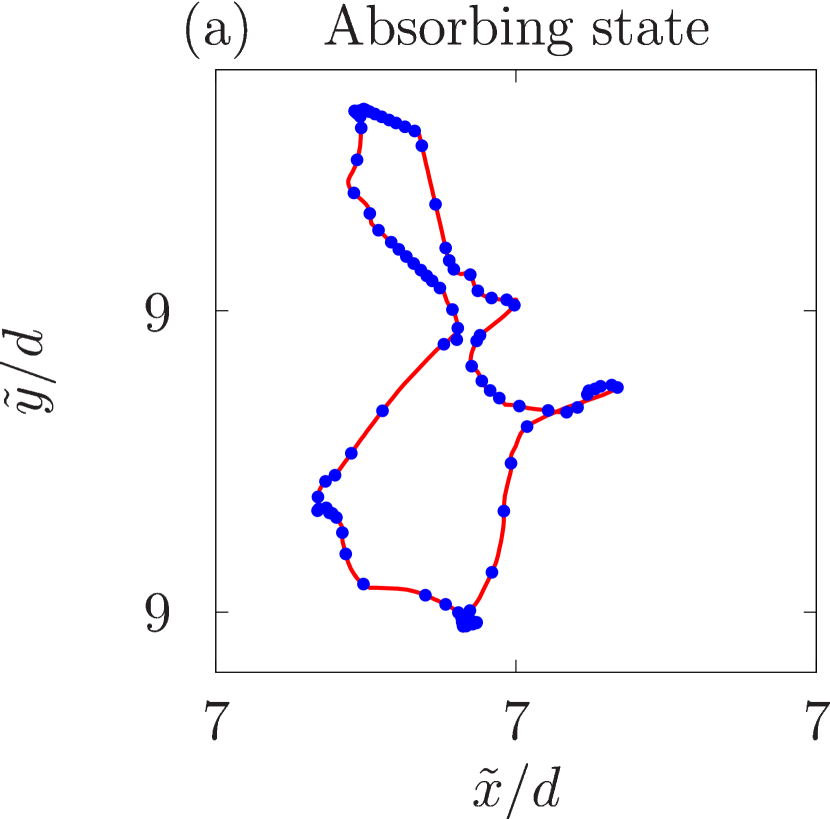
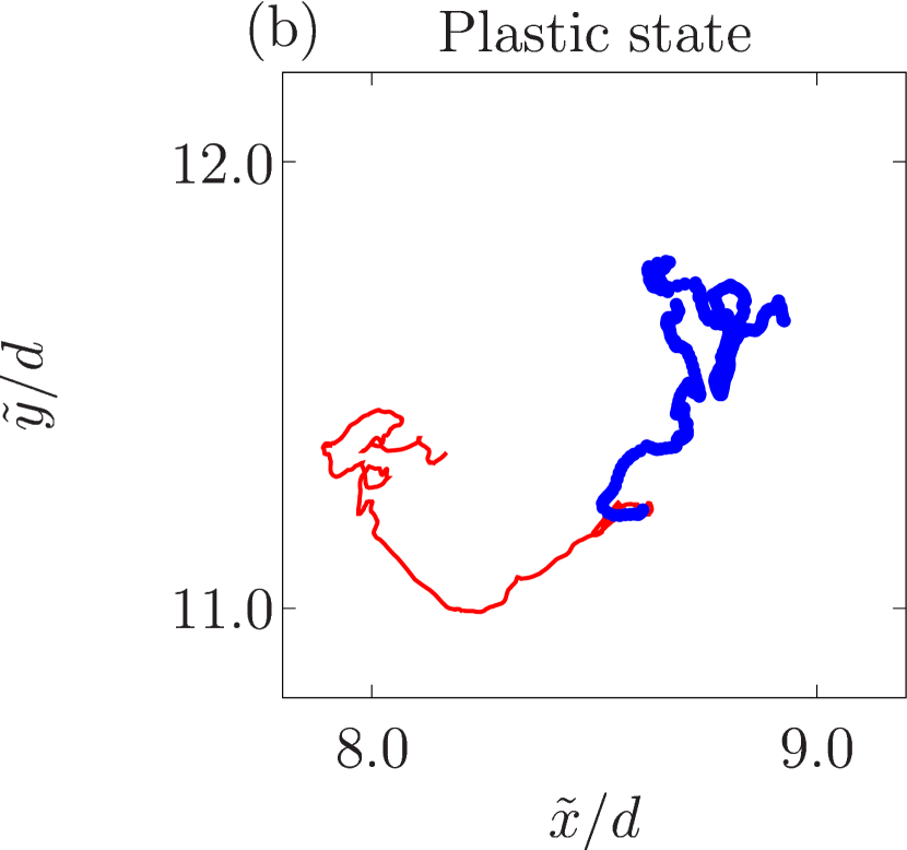
Figure 1: Non-affine particle trajectories in the last two cycles for $\gamma_{0}=0.02$ (a) and $0.1$ (b) with $\omega=10^{-4}\tau_{0}^{-1}$ and $\phi=0.87$, which corresponds to $\phi-\phi_{J}=0.029$. The circles represent the trajectory in the last cycle. The line represents the trajectory in the second to the last cycle.

Shear Modulus— We plot the storage modulus $G^{\prime}$ against the strain amplitude $\gamma_{0}$ for $\omega=10^{-4}\tau_{0}^{-1}$ with $\phi=0.870,0.860,0.850,$ and $0.845$ in Fig. 2. The yielding points to distinguish the absorbing state from the plastic state for various $\phi$ are shown by open pentagons Supple . The storage modulus $G^{\prime}$ decreases as $\gamma_{0}$ increases, but the yielding point is not identical to the point where $G^{\prime}$ starts to decrease. We call the decrease for $\gamma_{0}<\gamma_{c}$, the yielding strain amplitude, the softening in the absorbing state (SAS). We also call the decrease for $\gamma_{0}>\gamma_{c}$ the softening in the plastic state (SPS). It is remarkable that SAS is continuously connected to SPS, while a shoulder in $G^{\prime}$ appears in SPS for $0.04\leq\gamma_{0}\leq 0.1$ with $\phi=0.845$. In the inset of Fig. 2, we demonstrate that $G^{\prime}$ and $\gamma_{0}$ can be scaled by $\sqrt{\phi-\phi_{J}}$ and $\phi-\phi_{J}$, respectively, as indicated in Refs. OHern02 ; Bohy . We have confirmed that $G^{\prime}$ is independent of $\omega$ for $\omega\leq 10^{-3}\tau_{0}^{-1}$.

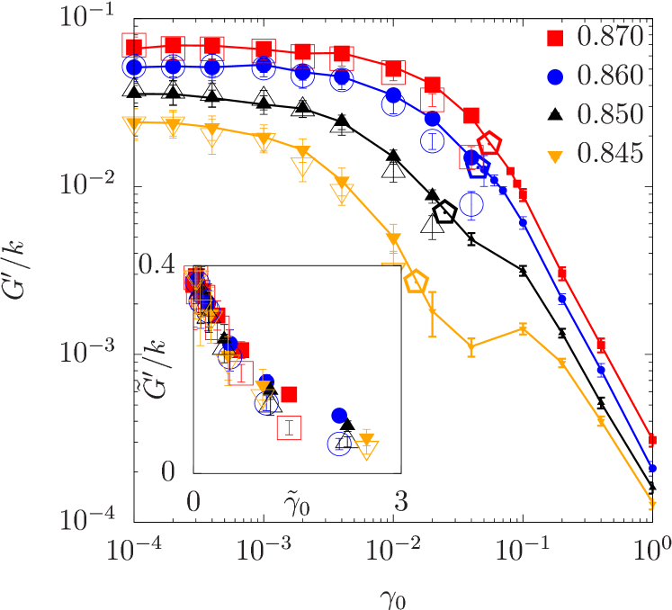
Figure 2: Storage modulus $G^{\prime}$ obtained in our simulation (filled symbols) against $\gamma_{0}$ for $\omega=10^{-4}\tau_{0}^{-1}$ with $\phi=0.870,0.860,0.850,$ and $0.845$, which corresponds to $\phi-\phi_{J}=0.029,0.019,0.009$, and $0.004$, respectively. The legends represent the packing fraction $\phi$. The data in the absorbing (plastic) state obtained in our simulation are shown in larger (smaller) filled symbols. The open pentagons represent the yielding strain amplitude $\gamma_{c}$, while other open symbols represent the theoretical expression using $G^{\prime}_{\rm T}$ in Eq. (14). (Inset) Scaled storage modulus $\tilde{G}^{\prime}=G^{\prime}/\sqrt{\phi-\phi_{J}}$ obtained in our simulation (filled symbols) and its theoretical expression using $G^{\prime}_{\rm T}$ (open symbols) in Eq. (14) against scaled strain amplitude $\tilde{\gamma}_{0}=\gamma_{0}/(\phi-\phi_{J})$ in the absorbing state.

Figure 3(a) displays the loss modulus $G^{\prime\prime}$ in the absorbing state against $\gamma_{0}$ for $\omega=10^{-4}\tau_{0}^{-1}$ with $\phi=0.870,0.860,0.850,$ and $0.845$, in which $G^{\prime\prime}$ does not strongly depend on $\phi$ and $\gamma_{0}$. See Ref. Supple for $G^{\prime\prime}$ in the plastic state. In Fig. 3(b), we plot the loss modulus $G^{\prime\prime}$ in the absorbing state against $\omega$ for $\phi=0.87$ with $\gamma=0.01$. Remarkably, $G^{\prime\prime}$ in Fig. 3(b) seems to converge to a non-zero value in the limit $\omega\to 0$, which contrasts with the behavior of the Kelvin–Voigt model (i.e., $G^{\prime\prime}\propto\omega$ Meyers ). This behavior indicates that dissipation remains even in the quasi-static limit in the absorbing state. Note that $G^{\prime\prime}\propto\omega$ is recovered when we adopt a sufficiently small $\gamma_{0}$ Supple .

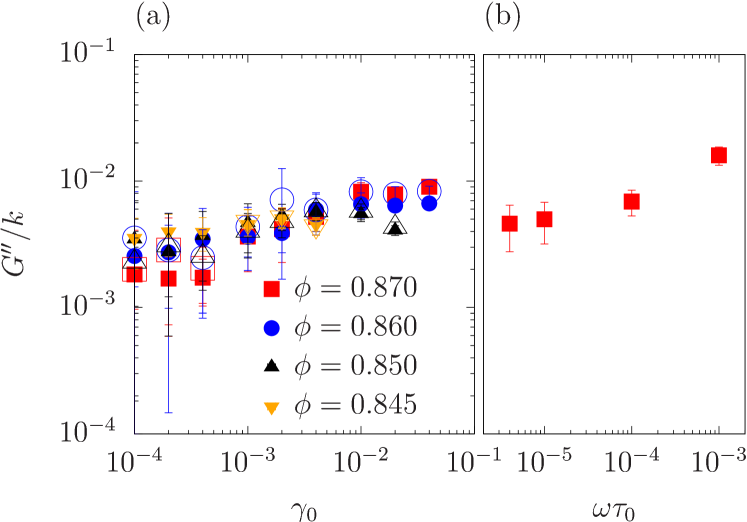
Figure 3: (a) Loss modulus $G^{\prime\prime}$ in the absorbing state obtained in our simulation (filled symbols) and its theoretical expression $G^{\prime\prime}_{\rm T}$ (open symbols) in Eq. (15) against $\gamma_{0}$ for $\omega=10^{-4}\tau_{0}^{-1}$ with $\phi=0.870,0.860,0.850,$ and $0.845$, which corresponds to $\phi-\phi_{J}=0.029,0.019,0.009$, and $0.004$, respectively. (b) Loss modulus $G^{\prime\prime}$ against $\omega\tau_{0}$ for $\phi=0.87$ with $\gamma_{0}=0.01$.

Fourier Analysis— In the absorbing state, the non-affine trajectory $\tilde{\bm{r}}_{i}(\theta)$ of particle $i$ can be expressed in a Fourier series as

$$\tilde{\bm{r}}_{i}(\theta)=\bm{R}_{i}+\sum_{n=1}^{\infty}\left(\bm{a}_{i}^{(n)}\sin n\theta+\bm{b}_{i}^{(n)}\cos n\theta\right)$$ (8)

with the center of the trajectory

$$\bm{R}_{i} = (X_{i},Y_{i})=\frac{1}{2\pi}\int_{0}^{2\pi}\ d\theta\ \tilde{\bm{r}}_{i}(\theta),$$ (9)

and the Fourier coefficients

$$\bm{a}_{i}^{(n)} = \frac{1}{\pi}\int_{0}^{2\pi}\ d\theta\ \sin n\theta\ \tilde{\bm{r}}_{i}(\theta),$$ (10)

$$\bm{b}_{i}^{(n)} = \frac{1}{\pi}\int_{0}^{2\pi}\ d\theta\ \cos n\theta\ \tilde{\bm{r}}_{i}(\theta).$$ (11)

If $\bm{a}_{i}^{(n)}=\bm{b}_{i}^{(n)}=\bm{0}$ for all $n$, the particle motion is affine. When only $\bm{a}_{i}^{(1)}$ is non-zero, the non-affine trajectory is a straight line, as shown in Fig. 4(a). In contrast, the trajectory exhibits an ellipse when $\bm{b}_{i}^{(1)}$ is also non-zero, as shown in Fig. 4(b). A nontrivial trajectory, as shown in Fig. 1(a), contains modes with $n\geq 2$. See Ref. Supple for the relationship between the trajectories and the Fourier coefficients.

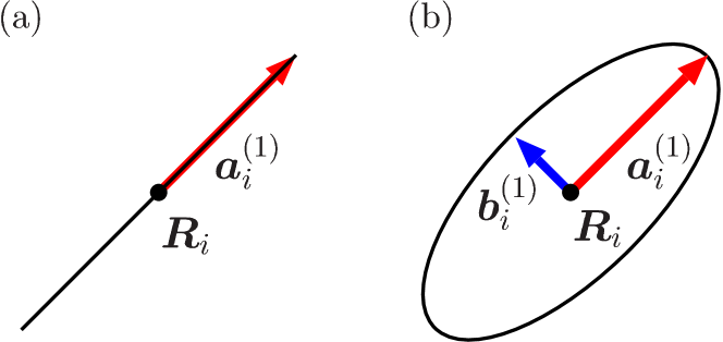
Figure 4: Schematics of the non-affine trajectory when only $\bm{a}_{i}^{(1)}$ is non-zero (a) and only $\bm{a}_{i}^{(1)}$ and $\bm{b}_{i}^{(1)}$ are non-zero (b).

In. Fig. 5(a), we plot the magnitudes of the Fourier components

$$a^{(n)}=\sum_{i}\left\langle\left|\bm{a}_{i}^{(n)}\right|\right\rangle/N,\ \ b^{(n)}=\sum_{i}\left\langle\left|\bm{b}_{i}^{(n)}\right|\right\rangle/N$$ (12)

obtained from our numerical data using Eqs. (10) and (11) against $n$ for $\phi=0.87$ and $\gamma_{0}=0.01$ with $\omega\tau_{0}=10^{-4}$ and $10^{-5}$. The Fourier components do not strongly depend on $\omega$, which indicates that the nontrivial loops do not disappear in the limit $\omega\to 0$. For different $\phi>\phi_{J}$ and $\gamma_{0}\geq 10^{-3}$, we have confirmed that $a^{(1)}$ is always the largest Comment , the other modes are non-zero to make loops with non-zero areas, and the Fourier components are independent of $\omega$. In Fig. 5(b), we plot $a^{(n)}/\gamma_{0}$ and $b^{(n)}/\gamma_{0}$ against $\gamma_{0}$ for $\phi=0.87$ and $\omega\tau_{0}=10^{-4}$ with $n=1$, where $a^{(n)}/\gamma_{0}$ and $b^{(n)}/\gamma_{0}$ are almost independent of $\gamma_{0}$. This behavior is consistent with that for the number of contact changes Supple .

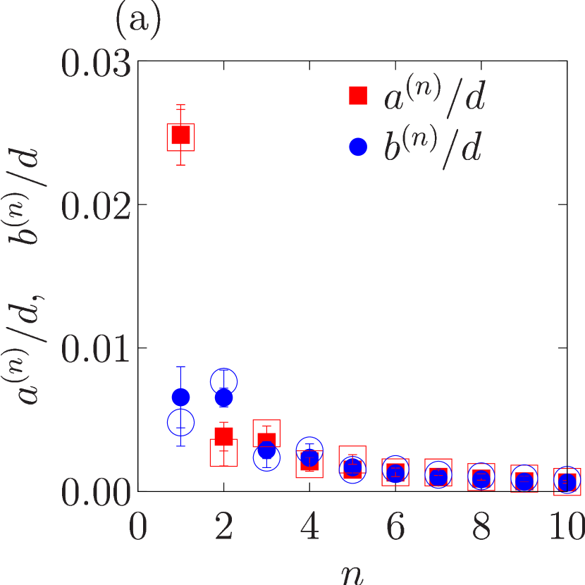
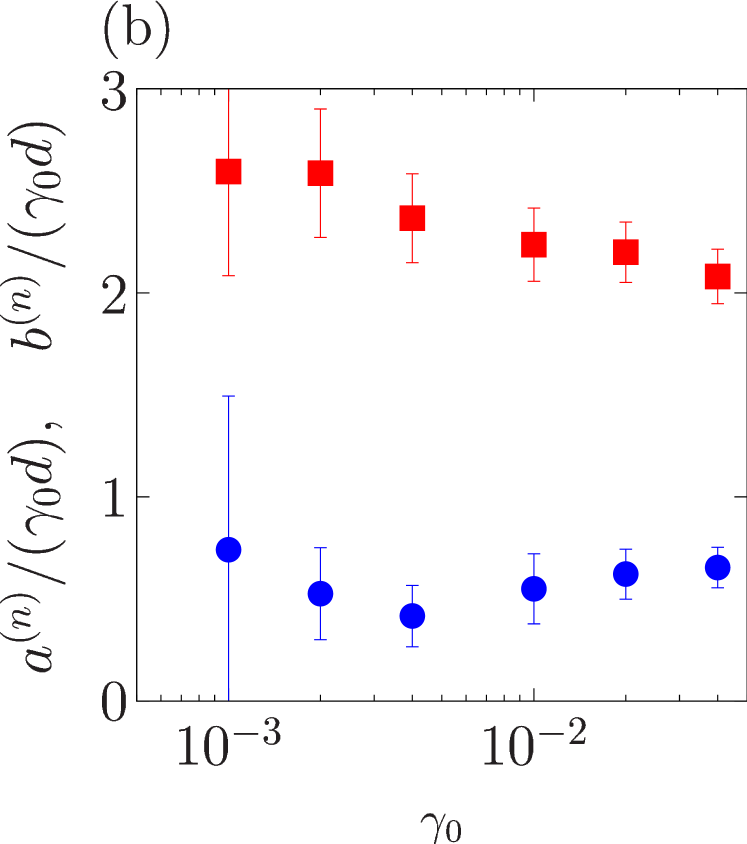
Figure 5: (a) Magnitudes of Fourier coefficients $a^{(n)}$ and $b^{(n)}$ against $n$ for $\phi=0.87$ and $\gamma_{0}=0.02$ with $\omega\tau_{0}=10^{-4}$ (filled symbols) and $10^{-5}$ (open symbols). (b) Magnitudes of the Fourier coefficients $a^{(n)}$ and $b^{(n)}$ normalized by $\gamma_{0}$ against $\gamma_{0}$ for $\phi=0.87$ and $\omega\tau_{0}=10^{-4}$ with $n=1$. $\phi=0.87$ corresponds to $\phi-\phi_{J}=0.029$.

Theoretical Analysis— Now, let us reproduce the numerical results by a simple analytic calculation. Substituting Eq. (8) into Eq. (7), ${\bm{r}}_{ij}(\theta)$ is given by

$${\bm{r}}_{ij}(\theta) = \bm{R}_{ij}+\gamma_{0}Y_{ij}\sin\theta\bm{e}_{x}$$ (13)

$$+\sum_{n=1}^{\infty}\left(\bm{a}_{ij}^{(n)}\sin n\theta+\bm{b}_{ij}^{(n)}\cos n\theta\right)$$

Here, we define $\bm{a}^{(n)}_{ij}=\bm{a}^{(n)}_{i}-\bm{a}^{(n)}_{j}$, $\bm{b}^{(n)}_{ij}=\bm{b}^{(n)}_{i}-\bm{b}^{(n)}_{j}$, and $\bm{R}_{ij}=(X_{ij},Y_{ij})=\bm{R}_{i}-\bm{R}_{j}$. Substituting Eq. (13) into Eq. (4) with Eq. (6) and neglecting the terms of $O(\gamma_{0})$, we obtain the expression $G^{\prime}_{\rm T}$ of the storage modulus in SAS as Supple

$$G^{\prime}_{\rm T} = -\frac{1}{L^{2}}\sum_{i,j}\left\langle\frac{X_{ij}^{2}Y_{ij}^{2}}{R_{ij}}\Psi^{\prime}(R_{ij})\right\rangle$$ (14)

$$-\frac{1}{L^{2}}\sum_{i,j}\left\langle Y_{ij}^{2}\Psi(R_{ij})\right\rangle$$

$$-\frac{1}{L^{2}}\sum_{i,j}\left\langle\left(\frac{a_{ij,x}^{(1)}}{\gamma_{0}}Y_{ij}+X_{ij}\frac{a_{ij,y}^{(1)}}{\gamma_{0}}\right)\Psi(R_{ij})\right\rangle$$

$$-\frac{1}{L^{2}}\sum_{i,j}\left\langle X_{ij}Y_{ij}\Psi^{\prime}(R_{ij})\frac{\bm{R}_{ij}\cdot\bm{a}_{ij}^{(1)}}{\gamma_{0}R_{ij}}\right\rangle,$$

where $\Psi(r)=-U^{\prime}(r)/r$. Here, we have assumed $|a_{i}^{(n)}|\sim|b_{i}^{(n)}|\sim\gamma_{0}$ and $\gamma_{0}\ll 1$. In the expression of Eq. (14), only the first harmonic contribution from $\bm{a}_{i}^{(1)}$ can survive because of Eq. (4). Note that $\bm{R}_{i}$ and $\bm{a}^{(1)}_{i}$ cannot be determined within the theory but are determined by our simulation data. In Fig. 2, we plot the theoretical prediction $G^{\prime}_{\rm T}$ as open symbols. The theoretical prediction quantitatively reproduces the numerical results except for large $\gamma_{0}$, which is out of the scope of our theory. The first and second terms on the right-hand side (RHS) of Eq. (14) represent the contributions from the affine transformation depending only on $\bm{R}_{i}$, while the third and fourth terms including $\bm{a}^{(1)}_{ij}/\gamma_{0}$ indicate the contributions from the non-affine trajectories. As shown in Ref. Supple , the contributions from the non-affine trajectories are almost independent of $\gamma_{0}$, which is consistent with the behavior of $a^{(1)}/\gamma_{0}$ shown in Fig. 5(b). Numerical evaluation in Ref. Supple reveals that SAS is dominated by the first term on RHS of Eq. (14) through the change of $\bm{R}_{i}$. The center of the non-affine trajectories $\bm{R}_{i}$ is changed by the rearrangement of the configuration during the transient to the absorbing state, which is consistent with the memory formation of dense particles during oscillatory shear Fiocco ; Paulsen ; Adhikari .

The theoretical expression $G^{\prime\prime}_{\rm T}$ of the loss modulus in SAS is given by Supple

$$G_{\rm T}^{\prime\prime} = -\frac{1}{L^{2}}\sum_{i,j}\left\langle\left(\frac{b_{ij,x}^{(1)}}{\gamma_{0}}Y_{ij}+X_{ij}\frac{b_{ij,y}^{(1)}}{\gamma_{0}}\right)\Psi(R_{ij})\right\rangle$$ (15)

$$-\frac{1}{L^{2}}\sum_{i,j}\left\langle X_{ij}Y_{ij}\Psi^{\prime}(R_{ij})R_{ij}\frac{\bm{R}_{ij}\cdot\bm{b}_{ij}^{(1)}}{\gamma_{0}R_{ij}^{2}}\right\rangle,$$

where we have used the same assumption to obtain Eq. (14). Similar to the case of $G_{T}^{\prime}$, only the contribution of the first harmonics $\bm{b}_{i}^{(1)}$ in the expression of Eq. (8) can survive because of Eq. (5). Note that $\bm{b}_{i}^{(1)}$ cannot be determined within the theory but is evaluated by the simulation data. The loss modulus depends only on the non-affine contribution including ${\bm{b}}_{i}^{(1)}$. The amplitude $b^{(1)}$ remains non-zero in the limit $\omega\to 0$, which leads to the residual loss modulus as in Fig. 3(b). We plot the theoretical expression $G^{\prime\prime}_{\rm T}$ using the open symbols in Fig. 3(a). $G^{\prime\prime}_{\rm T}$ also reproduces the numerical results except for large $\gamma_{0}$. Thus, our theory reveals the quantitative relationship between the loss modulus and closed trajectories, which was suggested in Ref. Keim14 .

Conclusion— We numerically studied the mechanical response of jammed materials consisting of frictionless and overdamped particles under oscillatory shear. The shear modulus exhibits SAS and the residual loss modulus exists in the quasi-static limit in the absorbing state. Through Fourier analysis of the closed trajectories, the theoretical expressions for the storage and loss moduli quantitatively agree with the numerical results.

Reference Tighe11 reported that the loss modulus vanishes in the absorbing jammed states in the limit $\omega\to 0$, which is inconsistent with our result. It is noteworthy that Ref. Tighe11 did not consider any transient state associated with contact changes before the system reaches the absorbing state. Since the loss modulus is expected to be given by the generalized Green-Kubo formula Chong ; Hayakawa , the origin of the residual loss modulus might be plastic events in the transient dynamics.

Recent studies of large amplitude oscillatory shear (LAOS) reveal that there are contributions from higher harmonics in the mechanical response of nonlinear viscoelastic materials Wagner ; Hyun . We calculate nonlinear viscoelastic moduli $G^{\prime}_{n}$ and $G^{\prime\prime}_{n}$ with $n\geq 2$ and confirm that such higher order moduli are negligible in our system as shown in Ref. Supple .

In this Letter, we focus only on the nonlinear response of disordered frictionless particles. However, even frictional grains and exhibit SAS depending on the friction coefficient Otsuki21 . Therefore, an extension of our theory to these systems will be our future work.

Supplemental Material:

This Supplemental Material provides some details that are not written in the main text. The results for underdamped frictionless granular particles without background friction are presented in Sec. I. In Sec. II, we show the dependence of $G^{\prime}$ and $G^{\prime\prime}$ on the number of particles $N$ and the number of cycles $n_{c}$. In Sec. III, we present the time evolution of the displacements of particles before reaching the absorbing state and the evaluation of the yielding strain amplitude $\gamma_{c}$. In Sec. IV, we illustrates the time evolutions of the stress-strain curves in the absorbing and plastic states. In Sec. V, we show how particle trajectories depend on $\gamma_{0}$ and $\omega$. In Sec. VI, we show that trajectories in the absorbing state with longer periods do not affect our theoretical results based on the absorbing trajectories whose periods are identical to the period of the external oscillation. In Sec. VII, we present the loss modulus in the absorbing and plastic states. In Sec. VIII, we demonstrate how the naive result of the Kelvin–Voigt model can be recovered for sufficiently small strain amplitude. In Sec. IX, we illustrate the relation between the Fourier coefficients and the shape of particle trajectories. In Sec. X, we show the number of contact changes during the last cycle in the absorbing state. In Sec. XI, we derive Eqs. (14) and (15) in the main text. In Sec. XII, we decompose the storage and loss moduli into several components, and clarify what components are dominant contributions for the storage and loss moduli. In Sec. XIII, we show the nonlinear viscoelastic moduli in our system to clarify the roles of higher harmonics.

I Underdamped granular particles

In this section, we show that our results are qualitatively unchanged in underdamped frictionless granular particles without background friction. Here, we use the SLLOD equation given by [34]

$$\frac{d}{dt}{\bm{r}}_{i} = \dot{\gamma}(t)y_{i}\bm{e}_{x}+\bm{p}_{i},$$ (S1)

$$\frac{d}{dt}{\bm{p}}_{i} = -\dot{\gamma}(t)p_{i,y}\bm{e}_{x}+\bm{F}_{i}$$ (S2)

under the Lees–Edwards boundary condition, where $\bm{p}_{i}=m(\dot{\bm{r}}_{i}-\dot{\gamma}(t)y_{i})\bm{e}_{x}$ and

$$\bm{F}_{i}=-\sum_{j\neq i}\frac{\partial}{\partial\bm{r}_{i}}U(r_{ij})-\sum_{j\neq i}\eta v^{\rm(n)}_{ij}\Theta(d_{ij}-r_{ij})\frac{\bm{r}_{ij}}{r_{ij}}$$ (S3)

with mass $m$, the interaction potential $U(r_{ij})$ given by Eq. (2), the viscous constant $\eta$, and the normal velocity

$$v^{\rm(n)}_{ij}=\left\{\frac{d}{dt}\bm{r}_{i}-\frac{d}{dt}\bm{r}_{j}\right\}\cdot\frac{\bm{r}_{ij}}{r_{ij}}.$$ (S4)

We adopt $\eta=\sqrt{mk}$. This model corresponds to frictionless granular particles with the restitution coefficient $e=0.043$. We adopt the leapfrog algorithm using the time step $\Delta t=0.05t_{0}$ with the characteristic time with $t_{0}=\sqrt{m/k}$.

In Fig. S1, we plot non-affine trajectories in the last two cycles for a particle with $\gamma_{0}=0.02$, $\phi=0.87$, and $\omega=10^{-4}\tau_{0}^{-1}$ in the absorbing state. The trajectories are closed, but there is a region where the position of the particle depends on the number of cycles $n_{c}$. The result of Fig. S1 is a typical one from the inertia effect in the underdamped system.

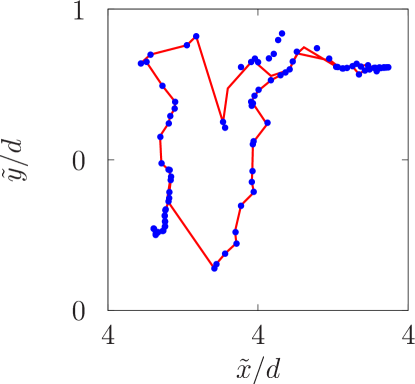
Figure S1: Non-affine trajectories in the last two cycles for underdamped particles with $\gamma_{0}=0.02$, $\phi=0.87$, and $\omega=10^{-4}\tau_{0}^{-1}$ in the absorbing state. The circles represent the trajectory in the last cycle. The line represents the trajectory in the second to the last cycle.

Figure S2 plots the magnitude of the Fourier coefficients $a^{(n)}$ and $b^{(n)}$ against $n$ for $\phi=0.87$ and $\gamma_{0}=0.02$ with $\omega\tau_{0}=10^{-4}$. As in the overdamped system, $a^{(1)}$ takes the largest value, and the other components are non-zero. In the inset of Fig. S2, we show $a^{(1)}$ and $b^{(1)}$ against $\gamma_{0}$ for $\phi=0.87$ and $\gamma_{0}=0.02$ with $\omega\tau_{0}=10^{-4}$, which are proportional to $\gamma_{0}$.

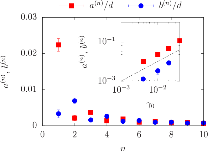
Figure S2: Magnitudes of Fourier coefficients $a^{(n)}$ and $b^{(n)}$ of the underdamped particles against $n$ for $\phi=0.87$ and $\gamma_{0}=0.02$ with $\omega\tau_{0}=10^{-4}$. (Inset) Magnitudes of the Fourier coefficients $a^{(n)}$ and $b^{(n)}$ against $\gamma_{0}$ for $\phi=0.87$ and $\omega\tau_{0}=10^{-4}$ with $n=1$. The dashed line represents $a^{(n)},b^{(n)}\propto\gamma_{0}$.

In Fig. S3, we plot the scaled storage modulus $G^{\prime}$ of the underdamped particles in the absorbing state against the scaled amplitude $\gamma_{0}$ for $\omega=10^{-4}\tau_{0}^{-1}$ with $\phi=0.870$ and $0.860$. The storage modulus exhibits SAS. The corresponding theoretical expression $G^{\prime}_{\rm T}$ in Eq. (14) as open symbols is also presented in Fig. S3, which quantitatively reproduces the numerical results except for the region of quite large $\gamma_{0}$

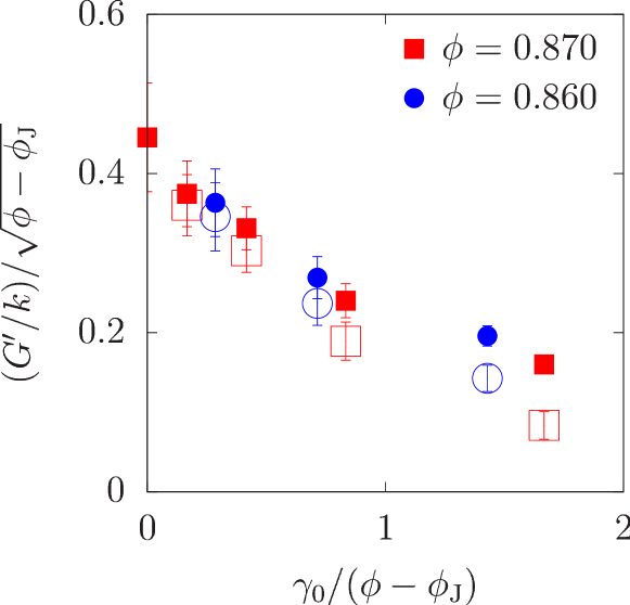
Figure S3: Scaled storage modulus $G^{\prime}/\sqrt{\phi-\phi_{J}}$ of underdamped particles (filled symbols) and its theoretical expression using $G^{\prime}_{\rm T}$ (open symbols) in Eq. (14) against scaled $\gamma_{0}/(\phi-\phi_{J})$ in the absorbing state scaled by the distance $\phi-\phi_{J}$ from the jamming point for $\omega=10^{-4}\tau_{0}^{-1}$ with $\phi=0.870$ and $0.860$.

In Fig. S4(a), we present the loss modulus $G^{\prime\prime}$ obtained in our simulation and its theoretical expression $G^{\prime\prime}_{\rm T}$ in Eq. (15) against $\gamma_{0}$ for $\omega=10^{-4}\tau_{0}^{-1}$ with $\phi=0.870$ and $0.860$ in the underdamped system. The loss modulus $G^{\prime\prime}$ does not strongly depend on $\phi$ and $\gamma_{0}$, and the theoretical expression $G^{\prime\prime}_{\rm T}$ reproduces the numerical results. In Fig. S4(b), we plot the loss modulus $G^{\prime\prime}$ against $\omega$ for $\phi=0.87$ with $\gamma=0.01$. The loss modulus seems to converge to a non-zero value in the limit $\omega\to 0$.

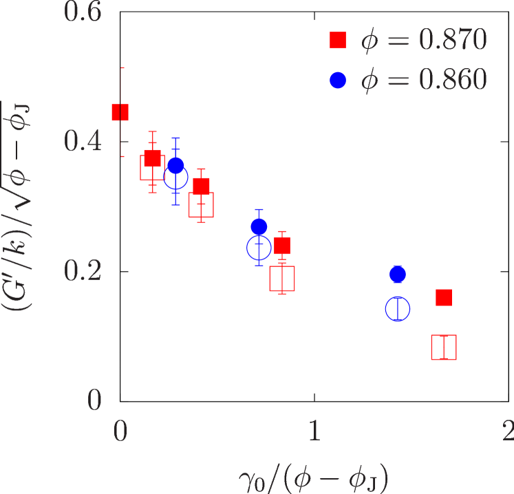
Figure S4: (a) Loss modulus $G^{\prime\prime}$ of underdamped particles obtained in our simulation (filled symbols) and its theoretical expression $G^{\prime\prime}_{\rm T}$ (open symbols) in Eq. (14) against $\gamma_{0}$ for $\omega=10^{-4}\tau_{0}^{-1}$ with $\phi=0.870$ and $0.860$. (b) Loss modulus $G^{\prime\prime}$ against $\omega$ for $\phi=0.87$ with $\gamma_{0}=0.01$.

The results in this section are consistent with those in the main text for the overdamped system. This indicates that the results presented in the main text are universal for jammed disordered materials.

II Dependence of $G^{\prime}$ and $G^{\prime\prime}$ on $N$ and $n_{c}$

In this section, we show the dependence of $G^{\prime}$ and $G^{\prime\prime}$ on the numbers of particles $N$ and cycles $n_{c}$ for the overdamped dynamics discussed in the main text. In Figs. S5(a) and (b), we plot $G^{\prime}$ and $G^{\prime\prime}$ against $\gamma_{0}$ for $\omega=10^{-4}\tau_{0}^{-1}$, $\phi=0.870$, and $n_{c}=20$ with $N=1000$ and $4000$, respectively. The shear moduli $G^{\prime}$ and $G^{\prime\prime}$ for $N=1000$ and $4000$ are consistent within error bars.

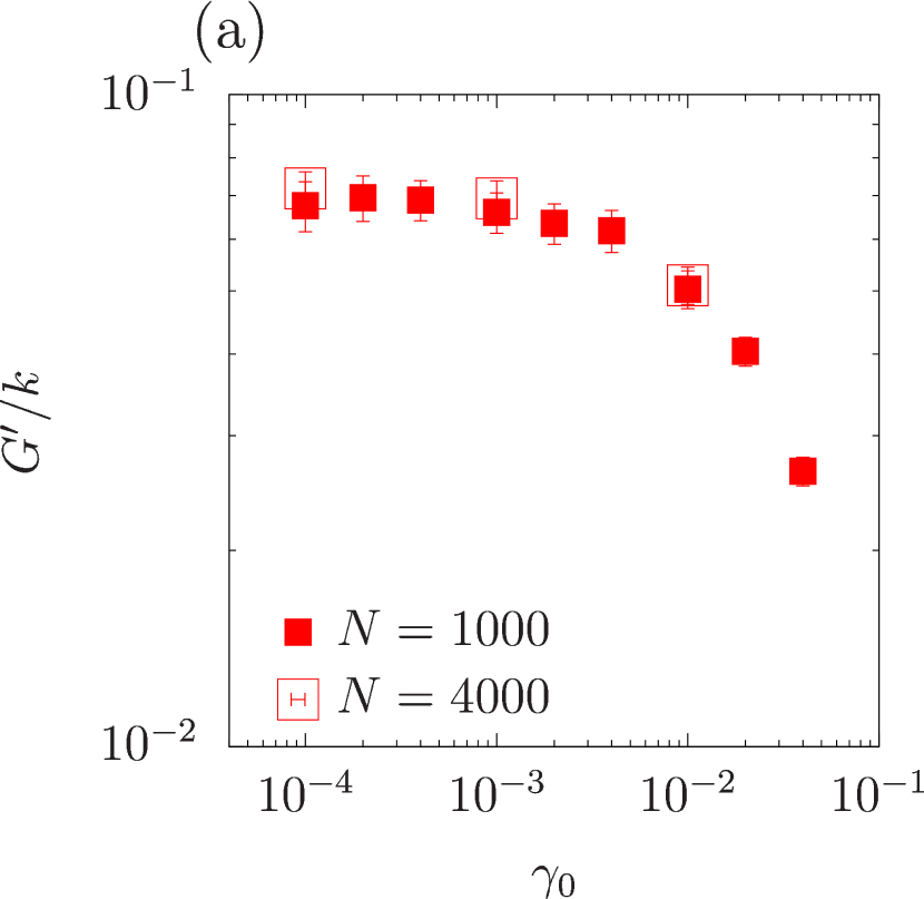
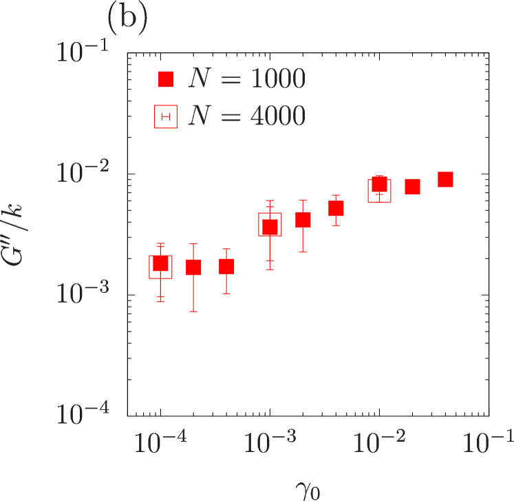
Figure S5: (a) Storage modulus $G^{\prime}$ against $\gamma_{0}$ for $\omega=10^{-4}\tau_{0}^{-1}$, $\phi=0.870$, and $n_{c}=20$ with $N=1000$ and $4000$. (b) Loss modulus $G^{\prime\prime}$ against $\gamma_{0}$ for $\omega=10^{-4}\tau_{0}^{-1}$, $\phi=0.870$, and $n_{c}=20$ with $N=1000$ and $4000$.

Figures S6(a) and (b) show $G^{\prime}$ and $G^{\prime\prime}$ against $n_{c}$ for $\omega=10^{-4}\tau_{0}^{-1}$, $\phi=0.870$, and $N=1000$ with $\gamma_{0}=0.02,0.04$, and $0.08$, respectively. The shear moduli $G^{\prime}$ and $G^{\prime\prime}$ reach statistical steady states for $n_{c}\geq 20$ within error bars.

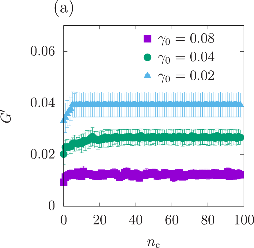
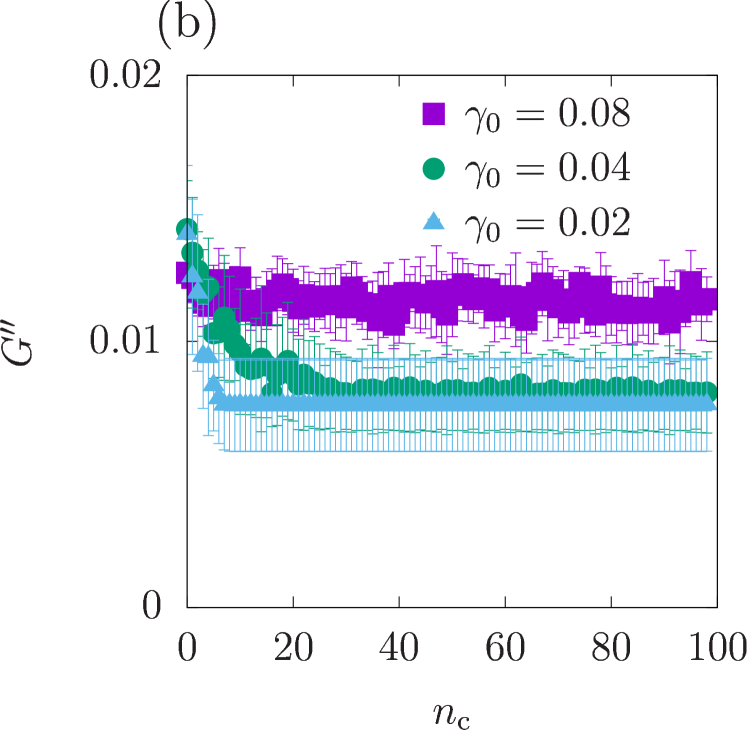
Figure S6: (a) Storage modulus $G^{\prime}$ against $n_{c}$ for $\omega=10^{-4}\tau_{0}^{-1}$, $\phi=0.870$, and $N=1000$ with $\gamma_{0}=0.02,0.04$, and $0.08$. (b) Loss modulus $G^{\prime\prime}$ against $n_{c}$ for $\omega=10^{-4}\tau_{0}^{-1}$, $\phi=0.870$, and $N=1000$ with $\gamma_{0}=0.02,0.04$, and $0.08$.

III Particle displacement and yielding strain amplitude

In this section, we show the time evolution of the displacements of particles before reaching the absorbing state and the evaluation of the yielding strain amplitude $\gamma_{c}$. Here, we introduce the particle displacement between $n_{c}$-th and $(n_{c}-m)$-th cycles as

$$dr_{m}(n_{c})=\sum_{i=1}^{N}\left|\bm{r}_{i}(n_{c}T)-\bm{r}_{i}((n_{c}-m)T)\right|/N$$ (S5)

with the period $T=2\pi/\omega$. We define $dr(n_{c})$ as the minimum value of $dr_{m}(n_{c})$ for $m$. In Fig. S7, we plot $dr(n_{c})$ against $n_{c}$ for $\omega=10^{-4}\tau_{0}^{-1}$ and $\phi=0.860$ with $\gamma_{0}=0.08,0.04$, and $0.02$. For $\gamma_{0}=0.08$, $dr(n_{c})$ remains non-zero, while it approaches $0$ after a transient for $\gamma_{0}=0.04$ and $0.02$. It is noteworthy that $dr(n_{c})$ reaches a steady state for $n_{c}>50$ in the case of $\gamma_{0}=0.04$, which is much larger than the steady $n_{c}$ in Fig. S6.

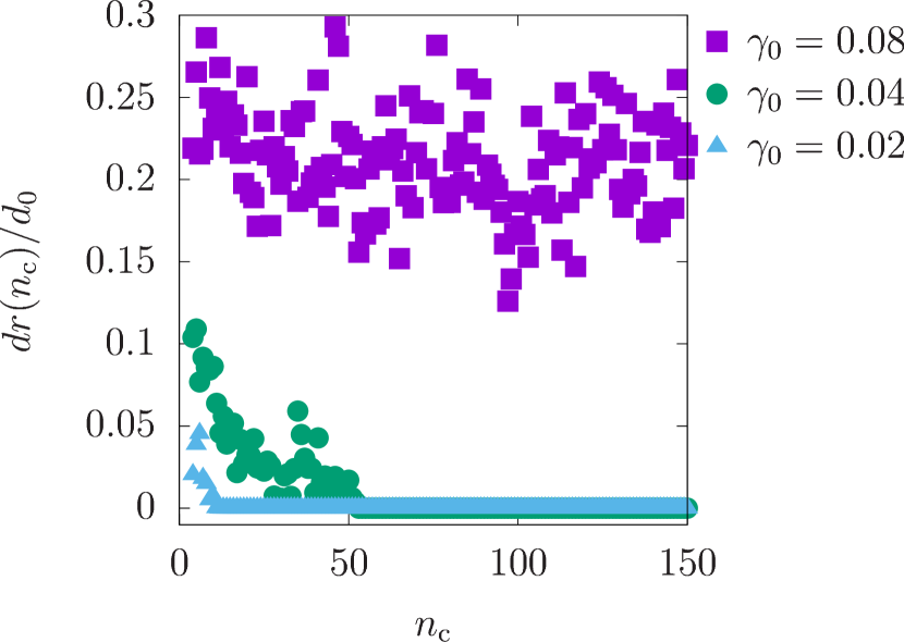
Figure S7: Displacements of particles $dr(n_{c})$ against $n_{c}$ for $\omega=10^{-4}\tau_{0}^{-1}$ and $\phi=0.860$ with $\gamma_{0}=0.08,0.04$, and $0.02$.

In Fig. S8, we plot $dr(n_{c})$ against $\gamma_{0}$ at $n_{c}=100$ for $\omega=10^{-4}\tau_{0}^{-1}$ with $\phi=0.870,0.860,0.850$ and $0.845$. For all $\phi$, $dr(n_{c})$ changes from $0$ to non-zero values as $\gamma_{0}$ increases. We call the absorbing state for $dr(n_{c})<d_{c}$ with smaller $\gamma_{0}$ and the plastic state for $dr(n_{c})>d_{c}$ with larger $\gamma_{0}$. The yielding strain amplitude $\gamma_{c}$ is defined as the boundary between these states. From Fig. S8, we estimate $0.04<\gamma_{c}<0.08$ for $\phi=0.870$, $0.04<\gamma_{c}<0.05$ for $\phi=0.860$, $0.02<\gamma_{c}<0.03$ for $\phi=0.850$, and $0.01<\gamma_{c}<0.02$ for $\phi=0.845$.

Figure S8: Displacement of particles $dr(n_{c})$ against $\gamma_{0}$ at $n_{c}=100$ for $\omega=10^{-4}\tau_{0}^{-1}$ with $\phi=0.870,0.860,0.850$ and $0.845$.

IV Stress-strain curve

In this section, we present typical stress strain curves in the absorbing and plastic states including their time evolution. Figure S9 displays the shear stress $\sigma$ against the strain $\gamma$ with $\gamma_{0}=0.02$ for different $n_{c}$. For $n_{c}\leq 5$, the stress-strain curves are not convergent, which indicate the system is in a transient state. For $n_{c}=6$ and $7$, the stress-strain curves become identical in the absorbing state. We plot the shear stress $\sigma$ against the strain $\gamma$ for $\gamma_{0}=0.1$ in Fig. S10. All the stress-strain curves are different for all $n_{c}$ because the system is in the plastic state.

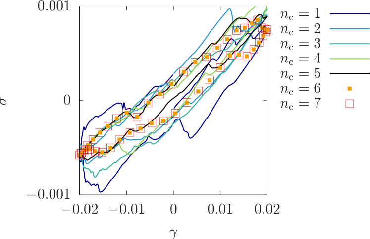
Figure S9: Plots of shear stress $\sigma$ against $\gamma$ for $\gamma_{0}=0.02$, $\omega=10^{-4}\tau_{0}^{-1}$, and $\phi=0.87$ corresponding to $\phi-\phi_{J}=0.029$ with various $n_{c}$.

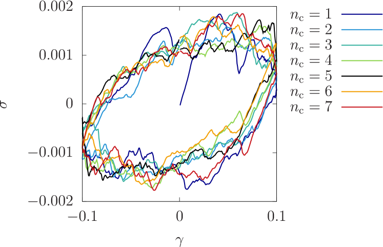
Figure S10: Plots of shear stress $\sigma$ against $\gamma$ for $\gamma_{0}=0.1$, $\omega=10^{-4}\tau_{0}^{-1}$ and $\phi=0.87$ corresponding to $\phi-\phi_{J}=0.029$ with various $n_{c}$.

V Dependence of trajectories on $\gamma_{0}$ and $\omega$

In this section, we present how particle trajectories depend on $\gamma_{0}$ and $\omega$. In Fig. S11, we plot the non-affine particle trajectories in the last cycle for $\omega=10^{-3}\tau_{0}^{-1}$ and $10^{-5}\tau_{0}^{-1}$ with $\phi=0.87$ and $\gamma_{0}=0.01$. Let us introduce

$${\bm{r}}^{\prime}_{i}=(x^{\prime}_{i},y^{\prime}_{i})=\tilde{\bm{r}}_{i}-{\bm{R}}_{i}.$$ (S6)

The trajectories form nontrivial loops, which remain for smaller $\omega$.

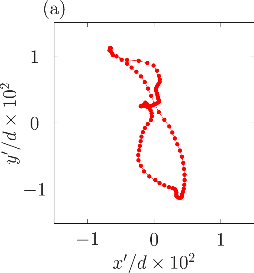
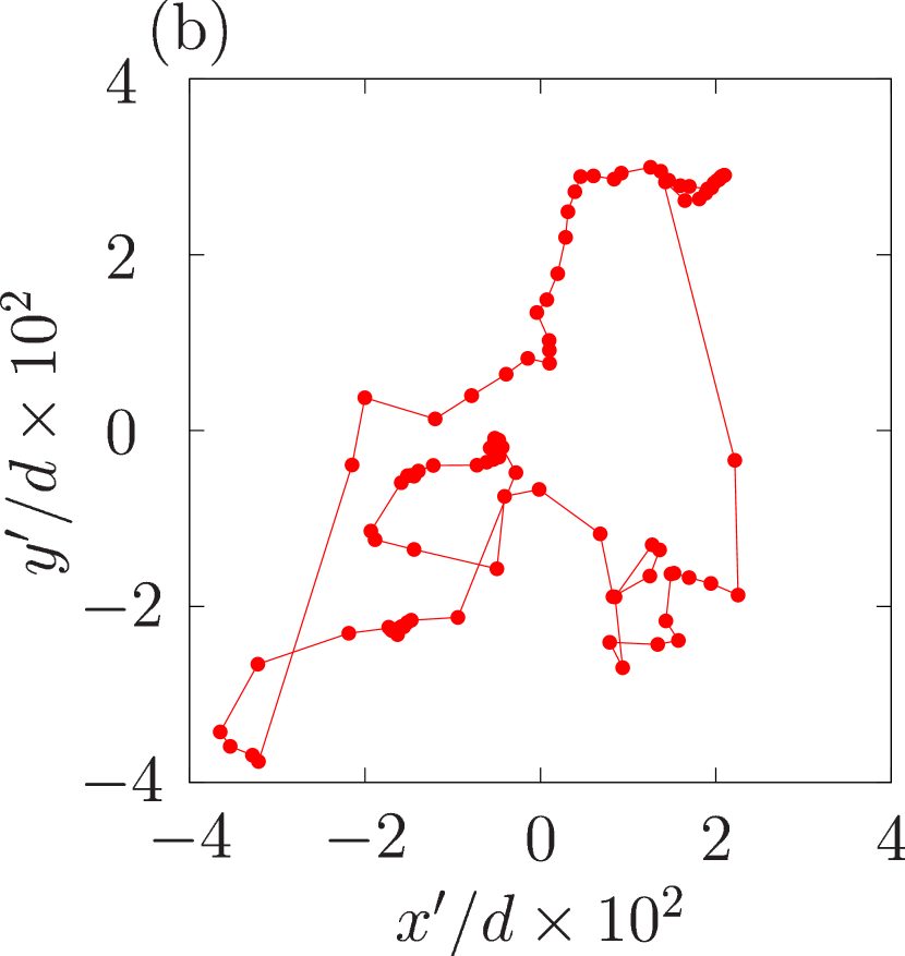
Figure S11: Non-affine particle trajectories in the last cycle for $\omega=10^{-3}\tau_{0}^{-1}$ (a) and $10^{-5}\tau_{0}^{-1}$ (b) with $\phi=0.87$ and $\gamma_{0}=0.01$.

Figure S12 represents the non-affine particle trajectories in the last cycle for $\omega=10^{-3}\tau_{0}^{-1}$ and $10^{-5}\tau_{0}^{-1}$ with $\phi=0.87$ and $\gamma_{0}=1.0\times 10^{-7}$. In Fig. S12 (a), the trajectory with $\omega=10^{-3}\tau_{0}^{-1}$ form an ellipse, but the trajectory becomes a straight line for $\omega=10^{-5}\tau_{0}^{-1}$ in Fig S12 (b).

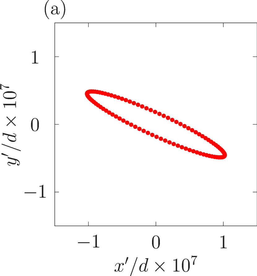
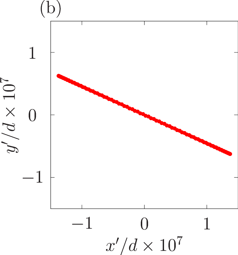
Figure S12: Non-affine particle trajectories in the last cycle for $\omega=10^{-3}\tau_{0}^{-1}$ (a) and $10^{-5}\tau_{0}^{-1}$ (b) with $\phi=0.87$ and $\gamma_{0}=1.0\times 10^{-7}$.

VI Effect of trajectories with longer periods

In this section, we discuss the effect of closed trajectories with periods longer than $2\pi$. As indicated by Refs. [27, 28, 30, 31, 33], some samples exhibit non-trivial absorbing trajectories where particles return to their original positions after more than one cycle of oscillatory shear. In these samples, the non-affine trajectories of a particle $\bm{r}_{i}(\theta)$ satisfy

$$\bm{r}_{i}(\theta)=\bm{r}_{i}(\theta+2M\pi)$$ (S7)

with $M=2,3,4,\cdots$. In this case, $\bm{r}_{i}(\theta)$ for $0<\theta<2M\pi$ is expressed in the Fourier series as

$$\tilde{\bm{r}}_{i}(\theta)=\bm{R}^{\prime}_{i}+\sum_{m=1}^{\infty}\left(\bm{A}_{i}^{(m)}\sin\frac{m\theta}{M}+\bm{B}_{i}^{(m)}\cos\frac{m\theta}{M}\right)$$ (S8)

with

$$\bm{R}^{\prime}_{i} = \frac{1}{2M\pi}\int_{0}^{2M\pi}\ d\theta\ \tilde{\bm{r}}_{i}(\theta),$$ (S9)

and the Fourier coefficients

$$\bm{A}_{i}^{(m)} = \frac{1}{M\pi}\int_{0}^{2M\pi}\ d\theta\ \sin\frac{m\theta}{M}\ \tilde{\bm{r}}_{i}(\theta),$$ (S10)

$$\bm{B}_{i}^{(m)} = \frac{1}{M\pi}\int_{0}^{2M\pi}\ d\theta\ \cos\frac{m\theta}{M}\ \tilde{\bm{r}}_{i}(\theta).$$ (S11)

However, in Eqs. (4) and (5), we need $\bm{r}_{i}(\theta)$ for $0\leq\theta<2\pi$ to calculate $G^{\prime}$ and $G^{\prime\prime}$. When $\bm{r}_{i}(\theta)$ is restricted to $0\leq\theta<2\pi$, we can use Eq. (8) with the Fourier coefficient given by Eqs. (10) and (11) as an expression of the trajectory, and we obtain the theoretical expressions Eqs. (14) and (15) even in this case. It should be noted that samples in the absorbing state with longer periods are rare, and the probability of emerging such a trajectory is smaller than $0.01$ for sufficiently packed systems above the jamming point, as shown in Ref. [30]. Therefore, we can ignore the effect of rare samples.

VII Loss modulus

In Fig. S13, we plot the loss modulus $G^{\prime\prime}$ against $\gamma_{0}$ for $\omega=10^{-4}\tau_{0}^{-1}$ with $\phi=0.870$ and $0.860$ including the data in the absorbing and plastic states. This figure corresponds to Fig. 3(a) in the main text, but Fig. S13 contains the data for a wide range of $\gamma_{0}$. The previous studies [21, 22] reported that the loss modulus has a peak around the yield strain for an underdamped system, but the peak of $G^{\prime\prime}$ is not clearly visible in our overdamped system.

Figure S13: Loss modulus $G^{\prime\prime}$ against $\gamma_{0}$ for $\omega=10^{-4}\tau_{0}^{-1}$ with $\phi=0.870$ and $0.860$. The larger (smaller) filled symbols represent the data in the absorbing (plastic) state. The open pentagons represent the yield strain amplitude $\gamma_{c}$.

VIII Shear modulus for small $\gamma_{0}$

In this section, we demonstrate that $G^{\prime}$ and $G^{\prime\prime}$ obey the Kelvin–Voigt model for a sufficiently small $\gamma_{0}$. Figure S14 is a set of plots of $G^{\prime}$ and $G^{\prime\prime}$ against $\omega\tau_{0}$ for $\phi=0.870$ and $\gamma_{0}=1.0\times 10^{-7}$, where $G^{\prime}$ is almost independent of $\omega$ and $G^{\prime\prime}$ is proportional to $\omega$. This behavior is consistent with that of the Kelvin–Voigt model.

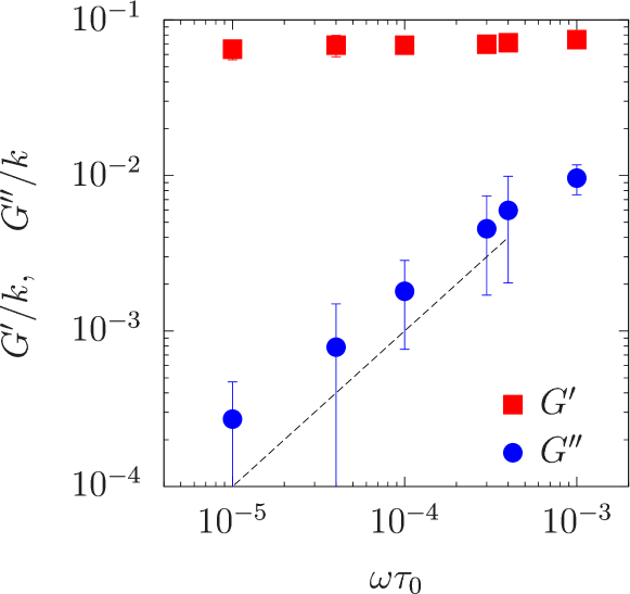
Figure S14: Plots of $G^{\prime}$ and $G^{\prime\prime}$ against $\omega$ for $\phi=0.870$ and $\gamma_{0}=1.0\times 10^{-7}$. The dashed line represents $G^{\prime\prime}\propto\omega$.

IX Relationship between closed trajectories and the Fourier coefficients

In this section, we present how the trajectory of a particle depends on the Fourier coefficients. Figure S15 compares the trajectory of a particle corresponding to Fig. 1(a) with its approximate trajectory using Eq. (8) with some restricted modes, where we estimate the coefficients using the true trajectory. In Fig. S15 (a), we plot the approximate trajectory (blue filled circles) using only $\bm{a}_{i}^{\rm(1)}$, where we set the other coefficients to $0$. The approximate trajectory (blue filled circles) is a straight line. Figure S15 (b) shows the approximate trajectory using $\bm{a}_{i}^{\rm(1)}$ and $\bm{b}_{i}^{\rm(1)}$, where the trajectory becomes an ellipse. As we increase the number of modes, the approximate trajectory approaches the true trajectory, as shown in Figs. S15 (c) and (d).

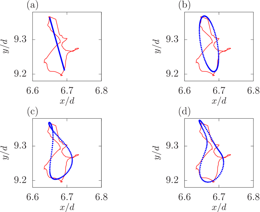
Figure S15: Trajectory shown in Fig. 1(a) of the main text and its approximate trajectories with some restricted modes. The red solid lines represent the original data, and the blue filled circles represent the approximate trajectory using (a) $\bm{a}_{i}^{\rm(1)}$, (b) $\bm{a}_{i}^{\rm(1)}$ and $\bm{b}_{i}^{\rm(1)}$, (c) $\bm{a}_{i}^{\rm(n)}$ and $\bm{b}_{i}^{\rm(n)}$ with $n=1$ and $2$, and (d) $\bm{a}_{i}^{\rm(n)}$ and $\bm{b}_{i}^{\rm(n)}$ with $n=1,2,$ and $3$.

X Cyclic contact changes

In this section, we show the number of contact changes during the last cycle in the absorbing state. References [21, 23, 25, 26] demonstrate that the nontrivial loops originate from cyclic open and close contacts. Here, we define $N_{cc}$ as the number of events where the same contact opens and closes again during the last cycle. In Fig. S16, we present $N_{\rm cc}$ during the last cycle for $\omega=10^{-4}\tau_{0}^{-1}$ with $\phi=0.870$ against $\gamma_{0}$ in the absorbing state. The number of cyclic contact changes $N_{\rm cc}$ is nearly proportional to $\gamma_{0}$. This dependence is consistent with the behaviors of $a^{(n)}$ and $b^{(n)}$ of the Fourier components, which are almost proportional to $\gamma_{0}$.

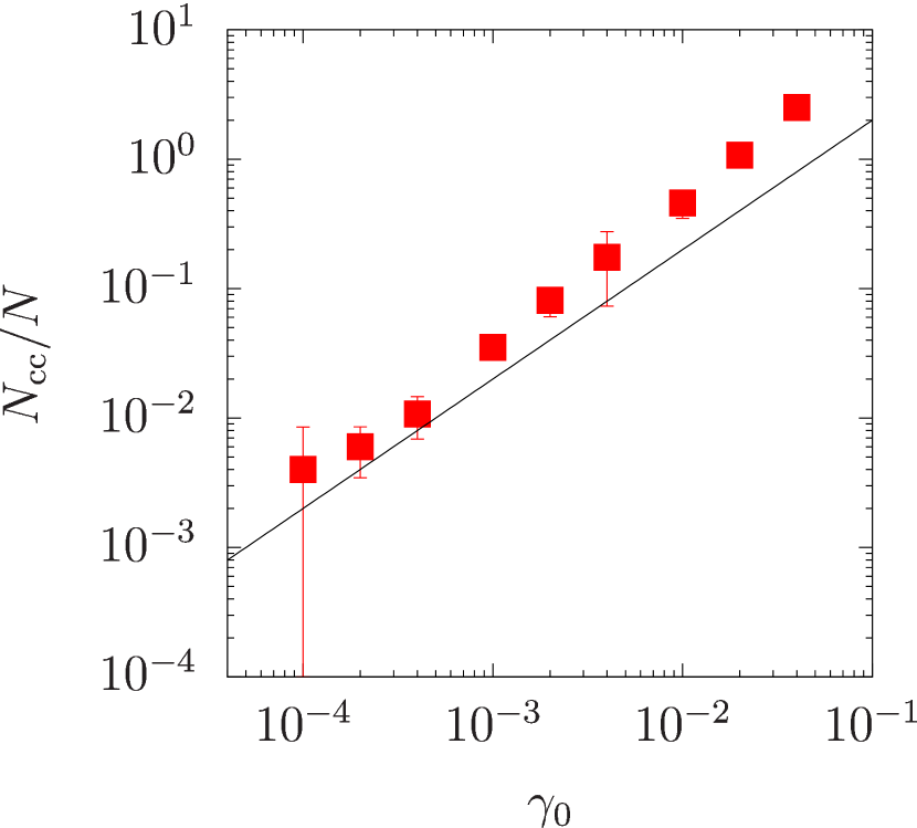
Figure S16: The number of cyclic contact changes $N_{\rm cc}$ during the last cycle for $\omega=10^{-4}\tau_{0}^{-1}$ with $\phi=0.870$ against $\gamma_{0}$. The solid line represents $N_{\rm cc}\sim\gamma_{0}$.

XI Details of the theoretical analysis

In this section, we derive Eqs. (14) and (15) in the main text by assuming $|a_{i}^{(n)}|\sim|b_{i}^{(n)}|\sim\gamma_{0}$ and $\gamma_{0}\ll 1$. From Eq. (13) in the main text, $x_{ij}(\theta)$ and $y_{ij}(\theta)$ are given by

$$x_{ij}=X_{ij}+\gamma_{0}\sin\theta Y_{ij}+\sum_{n=1}^{\infty}\left(a_{ij,x}^{(n)}\sin n\theta+b_{ij,x}^{(n)}\cos n\theta\right),$$ (S12)

$$y_{ij}=Y_{ij}+\sum_{n=1}^{\infty}\left(a_{ij,y}^{(n)}\sin n\theta+b_{ij,y}^{(n)}\cos n\theta\right),$$ (S13)

where $\bm{a}^{(n)}_{ij}=(a_{ij,x}^{(n)},a_{ij,y}^{(n)})=\bm{a}^{(n)}_{i}-\bm{a}^{(n)}_{j}$, $\bm{b}^{(n)}_{ij}=(b_{ij,x}^{(n)},b_{ij,y}^{(n)})=\bm{b}^{(n)}_{i}-\bm{b}^{(n)}_{j}$. Using this equation and neglecting the terms of $O(\gamma_{0}^{2})$, $|\bm{r}_{ij}(\theta)|^{2}=x_{ij}^{2}+y_{ij}^{2}$ is given by

$$|\bm{r}_{ij}(\theta)|^{2}\simeq R_{ij}^{2}\left\{1+2E_{ij}(\theta)\right\}$$ (S14)

with

$$E_{ij}(\theta) = \sum_{n=1}^{\infty}\frac{\bm{R}_{ij}\cdot\bm{a}_{ij}^{(n)}}{R_{ij}^{2}}\sin n\theta+\sum_{n=1}^{\infty}\frac{\bm{R}_{ij}\cdot\bm{b}_{ij}^{(n)}}{R_{ij}^{2}}\cos n\theta$$ (S15)

$$+\gamma_{0}\frac{X_{ij}Y_{ij}}{R_{ij}^{2}}\sin\theta.$$

From Eq. (S14), $r_{ij}(\theta)$ is approximately obtained as

$$r_{ij}(\theta)\simeq R_{ij}\left\{1+E_{ij}(\theta)\right\}$$ (S16)

up to $O(\gamma_{0})$. Using this equation, we obtain $\Psi(r)=-U^{\prime}(r)/r$ up to $O(\gamma_{0})$ as

$$\Psi(r_{ij}(\theta)) \simeq \Psi(R_{ij})+\Psi^{\prime}(R_{ij})R_{ij}E_{ij}(\theta).$$ (S17)

Substituting Eqs. (S12)–(S17) into Eq. (6), we obtain

$$\sigma(\theta) = -\frac{1}{L^{2}}\sum_{(i,j)}\left\{\Psi(R_{ij})+\Psi^{\prime}(R_{ij})R_{ij}E_{ij}(\theta)\right\}$$ (S18)

$$\times\left\{X_{ij}+\gamma_{0}\sin\theta Y_{ij}+\sum_{n=1}^{\infty}\left(a_{ij,x}^{(n)}\sin n\theta+b_{ij,x}^{(n)}\cos n\theta\right)\right\}$$

$$\times\left\{Y_{ij}+\sum_{n=1}^{\infty}\left(a_{ij,y}^{(n)}\sin n\theta+b_{ij,y}^{(n)}\cos n\theta\right)\right\}.$$

Here, we abbreviate $\displaystyle\sum_{i}\sum_{j>i}$ as $\displaystyle\sum_{(i,j)}$. Neglecting the terms of $O(\gamma_{0}^{2})$, $\sigma(\theta)$ is approximated as

$$\sigma(\theta) \simeq -\frac{1}{L^{2}}\sum_{(i,j)}X_{ij}Y_{ij}\Psi(R_{ij})-\frac{1}{L^{2}}\sum_{(i,j)}\gamma_{0}\sin\theta Y_{ij}^{2}\Psi(R_{ij})$$ (S19)

$$-\frac{1}{L^{2}}\sum_{(i,j)}\sum_{n=1}^{\infty}\left(a_{ij,x}^{(n)}\sin n\theta+b_{ij,x}^{(n)}\cos n\theta\right)Y_{ij}\Psi(R_{ij})$$

$$-\frac{1}{L^{2}}\sum_{(i,j)}\sum_{n=1}^{\infty}X_{ij}\left(a_{ij,y}^{(n)}\sin n\theta+b_{ij,y}^{(n)}\cos n\theta\right)\Psi(R_{ij})$$

$$-\frac{1}{L^{2}}\sum_{(i,j)}X_{ij}Y_{ij}\Psi^{\prime}(R_{ij})R_{ij}E_{ij}(\theta).$$

By substituting this equation into Eqs. (4) and (5) and using

$$\frac{1}{\pi}\int_{0}^{2\pi}\ d\theta\ \sin m\theta\sin n\theta=\delta_{mn},$$ (S20)

$$\frac{1}{\pi}\int_{0}^{2\pi}\ d\theta\ \sin m\theta\cos n\theta=0,$$ (S21)

we obtain Eqs. (14) and (15) in the main text.

XII Components of shear moduli

In this section, we clarify what terms of the theoretical expressions $G^{\prime}_{\rm T}$ and $G^{\prime\prime}_{\rm T}$ in the absorbing state in Eqs. (14) and (15) are dominant. Here, $G^{\prime}_{\rm T}$ consists of four terms as

$$G^{\prime}_{\rm T} = G^{\prime}_{{\rm T},1}+G^{\prime}_{{\rm T},2}+G^{\prime}_{{\rm T},3}+G^{\prime}_{{\rm T},4}$$ (S22)

with

$$G^{\prime}_{{\rm T},1} =-\frac{1}{L^{2}}\sum_{i,j}\left\langle\frac{X_{ij}^{2}Y_{ij}^{2}}{R_{ij}}\Psi^{\prime}(R_{ij})\right\rangle,$$ (S23)

$$G^{\prime}_{{\rm T},2} =-\frac{1}{L^{2}}\sum_{i,j}\left\langle Y_{ij}^{2}\Psi(R_{ij})\right\rangle,$$ (S24)

$$G^{\prime}_{{\rm T},3} =-\frac{1}{L^{2}}\sum_{i,j}\left\langle\left(\frac{a_{ij,x}^{(1)}}{\gamma_{0}}Y_{ij}+X_{ij}\frac{a_{ij,y}^{(1)}}{\gamma_{0}}\right)\Psi(R_{ij})\right\rangle,$$ (S25)

$$G^{\prime}_{{\rm T},4} =-\left\langle\frac{1}{L^{2}}\sum_{i,j}X_{ij}Y_{ij}\Psi^{\prime}(R_{ij})\frac{\bm{R}_{ij}\cdot\bm{a}_{ij}^{(1)}}{\gamma_{0}R_{ij}}\right\rangle,$$ (S26)

where $G^{\prime}_{{\rm T},1}$ and $G^{\prime}_{{\rm T},2}$ represent the contributions from the affine motion, respectively, while $G^{\prime}_{{\rm T},1}$ and $G^{\prime}_{{\rm T},2}$ are the contributions from the non-affine motion, respectively. In Fig. S17, we show $G^{\prime}_{{\rm T},n}$ in the absorbing state for $\omega=10^{-4}\tau_{0}^{-1}$ with $\phi=0.870$. We find that $G^{\prime}_{{\rm T},1}$ and $G^{\prime}_{{\rm T},4}$ are dominant. $G^{\prime}_{{\rm T},1}$ decreases with $\gamma_{0}$, while the other $G_{{\rm T},n}^{\prime}$ with $n=2,3,4$ are almost independent of $\gamma_{0}$. This indicates that SAS results from the behavior of $G^{\prime}_{{\rm T},1}$.

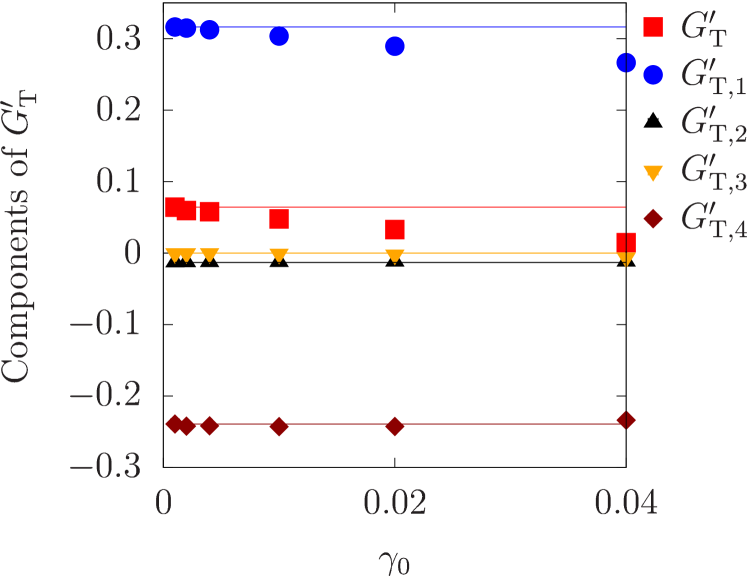
Figure S17: $G^{\prime}_{{\rm T},n}$ with $n=1,2,3$ and $4$ against $\gamma_{0}$ in the absorbing state for $\omega=10^{-4}\tau_{0}^{-1}$ with $\phi=0.870$. The horizontal lines represent $G^{\prime}_{{\rm T},n}$ in the limit $\gamma_{0}\to 0$, which is estimated at $\gamma_{0}=0.001$.

On the other hand, the loss modulus $G^{\prime\prime}_{\rm T}$ consists of two terms as

$$G_{\rm T}^{\prime\prime} = G_{{\rm T},1}^{\prime\prime}+G_{{\rm T},2}^{\prime\prime}$$ (S27)

with

$$G_{{\rm T},1}^{\prime\prime} =-\frac{1}{L^{2}}\sum_{i,j}\left\langle\left(\frac{b_{ij,x}^{(1)}}{\gamma_{0}}Y_{ij}+X_{ij}\frac{b_{ij,y}^{(1)}}{\gamma_{0}}\right)\Psi(R_{ij})\right\rangle,$$ (S28)

$$G_{{\rm T},2}^{\prime\prime} =-\frac{1}{L^{2}}\sum_{i,j}\left\langle X_{ij}Y_{ij}\Psi^{\prime}(R_{ij})R_{ij}\frac{\bm{R}_{ij}\cdot\bm{b}_{ij}^{(1)}}{\gamma_{0}R_{ij}^{2}}\right\rangle.$$ (S29)

In Fig. S17, we show $G^{\prime\prime}_{{\rm T},n}$ with $n=1$ and $2$ in the absorbing state for $\omega=10^{-4}\tau_{0}^{-1}$ with $\phi=0.870$. The result shows that $G^{\prime\prime}_{{\rm T},1}$ is dominant and almost independent of $\gamma_{0}$. $G^{\prime\prime}_{{\rm T},2}$ depends on $\gamma_{0}$, but it is much smaller than $G^{\prime\prime}_{{\rm T},1}$ for $\gamma_{0}<0.1$.

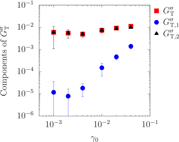
Figure S18: $G^{\prime}_{{\rm T},n}$ with $n=1$ and $2$ against $\gamma_{0}$ in the absorbing state for $\omega=10^{-4}\tau_{0}^{-1}$ with $\phi=0.870$.

XIII Non-linear viscoelastic moduli

In this section, we examine the non-liner viscoelastic moduli in our system. The nonlinear elastic response is generally characterized by nonlinear viscoelastic moduli $G^{\prime}_{n}$ and $G^{\prime\prime}_{n}$ satisfying [41, 42]

$$\sigma(t)=\gamma_{0}\sum_{n=1}\{G^{\prime}_{n}\sin(n\omega t)+G^{\prime\prime}_{n}\cos(n\omega t)\}.$$ (S30)

The storage and loss moduli are, respectively, given by $G^{\prime}=G^{\prime}_{1}$ and $G^{\prime\prime}=G^{\prime\prime}_{1}$. $G^{\prime}_{n}$ and $G^{\prime\prime}_{n}$ for $n\geq 2$ represent higher harmonics. In Figs. S19 and S20, we plot $G^{\prime}_{n}$ and $G^{\prime\prime}_{n}$ in the absorbing state for $\omega=10^{-4}\tau_{0}^{-1}$ and $\phi=0.870$ with $n=1,2$, and $3$, respectively. These figures indicate that the higher harmonics are negligible in our system.

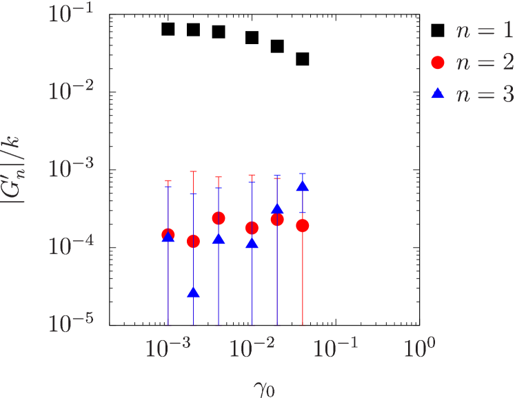
Figure S19: $G_{n}^{\prime}$ against $\gamma_{0}$ in the absorbing state for $\omega=10^{-4}\tau_{0}^{-1}$ and $\phi=0.870$ with $n=1,2$, and $3$.

Figure S20: $G_{n}^{\prime\prime}$ against $\gamma_{0}$ in the absorbing state for $\omega=10^{-4}\tau_{0}^{-1}$ and $\phi=0.870$ with $n=1,2$, and $3$.

References

(1) M. van Hecke, J. Phys. Condens. Matter 22, 033101 (2009)
(2) R. P. Behringer and B. Chakraborty, Rep. Prog. Phys. 82 012601 (2019)
(3) C. S. O’Hern, S. A. Langer, A. J. Liu, and S. R. Nagel, Phys. Rev. Lett. 88, 075507 (2002).
(4) B. P. Tighe, Phys. Rev. Lett. 107, 158303 (2011).
(5) M. Otsuki and H. Hayakawa, Phys. Rev. E 95, 062902 (2017).
(6) C. Coulais, A. Seguin, and O. Dauchot, Phys. Rev. Lett. 113, 198001 (2014).
(7) M. Otsuki and H. Hayakawa, Phys. Rev. E 90, 042202 (2014).
(8) K. Hima Nagamanasa, S. Gokhale, A. K. Sood, and R. Ganapathy, Phys. Rev. E 89, 062308 (2014).
(9) E. D. Knowlton, D. J. Pine, and L. Cipelletti, Soft Matter 10, 6931 (2014).
(10) T. Kawasaki and L. Berthier, Phys. Rev. E 94, 022615 (2016).
(11) P. Leishangthem, A. D. S. Parmar, and S. Sastry, Nat. Commun. 8, 14653 (2017).
(12) A. H. Clark, J. D. Thompson, M. D. Shattuck, N. T. Ouellette, and C. S. O’Hern, Phys. Rev. E 97, 062901 (2018).
(13) J. Boschan, S. Luding, and B. P. Tighe, Granul. Matter 21, 58 (2019).
(14) H. Hinrichsen, Adv. Phys. 49, 815 (2000).
(15) M. Henkel, H. Hinrichsen, and S. Lubeck, Non-equilibrium Phase Transition I: Absorbing Phase Transitions (Springer, Heidelberg, 2008).
(16) D. J. Pine, J. P. Collub, J. F. Brady, and A. M. Leshansky, Nature (London) 438, 997 (2005).
(17) L. Corté, P. M. Chaikin, J. P. Gollub, and D. J. Pine, Nature Phys. 4, 420 (2008).
(18) J. Boschan, D. Vågberg, E. Somfai, and B. P. Tighe, Soft Matter 12, 5450 (2016).
(19) D. Nakayama, H. Yoshino, and F. Zamponi,J. Stat. Mech. 2016 104001 (2016).
(20) T. Kawasaki and K. Miyazaki, arXiv:2003.10716.
(21) S. Dagois-Bohy, E. Somfai, B. P. Tighe, and M. van Hecke, Soft Matter 13, 9036 (2017).
(22) D. Ishima and H. Hayakawa, Phys. Rev. E 101, 042902 (2020).
(23) M. Lundberg, K. Krishan, N. Xu, C. S. O’Hern, and M. Dennin, Phys. Rev. E 77, 041505 (2008).
(24) C. F. Schreck, R. S. Hoy, M. D. Shattuck, and C. S. O’Hern, Phys. Rev. E 88, 052205 (2013).
(25) N. C. Keim and P. E. Arratia, Soft Matter 9, 6222 (2013).
(26) N. C. Keim and P. E. Arratia, Phys. Rev. Lett. 112, 028302 (2014).
(27) I. Regev, T. Lookman, and C. Reichhardt Phys. Rev. E 88, 062401 (2013).
(28) I. Regev, J. Weber, C. Reichhardt, K. A. Dahmen, and T. Lookman, Nat. Commun. 6, 8805 (2015).
(29) N. V. Priezjev, Phys. Rev. E 93, 013001 (2016).
(30) M. O. Lavrentovich, A. J. Liu, and S. R. Nagel, Phys. Rev. E 96, 020101(R) (2017).
(31) K. Nagasawa, K. Miyazaki and T. Kawasaki, Soft Matter 15, 7557 (2019).
(32) P. Das, H. A. Vinutha, and S. Sastry, Proc. Natl. Acad. Sci. USA 117, 10203 (2020).
(33) K. Khirallah, B. Tyukodi, D. Vandembroucq, and C. E. Maloney, Phys. Rev. Lett. 126, 218005 (2021).
(34) M. S. van Deen, J. Simon, Z. Zeravcic, S. Dagois-Bohy, B. P. Tighe, and M. van Hecke, Phys. Rev. E 90, 020202(R) (2014).
(35)
D. J. Evans and G. P. Morriss, Statistical Mechanics of Nonequilibrium Liquids 2nd ed. (Cambridge University Press, Cambridge, 2008).
(36) See Supplemental Material.
(37) M. Doi and S. F. Edwards, The Theory of Polymer Dynamics
(Oxford University Press, Oxford, 1986).
(38) M. Meyers and K. Chawla, Mechanical Behavior of Materials (Cambridge University Press, Cambridge, 2008).
(39) We suppose is the largest because the mode proportional to is synchronized with the external oscillation .
(40) D. Fiocco, G. Foffi, and S. Sastry, Phys. Rev. Lett. 112, 025702 (2014).
(41) J. D. Paulsen, N. C. Keim, and S. R. Nagel, Phys. Rev. Lett. 113, 068301 (2014).
(42) M. Adhikari and S. Sastry, Eur. Phys. J. E 41, 105 (2018).
(43) S-H. Chong, M. Otsuki, and H. Hayakawa, Phys. Rev. E 81, 041130 (2010).
(44) H. Hayakawa and M. Otsuki, Phys. Rev. E 88, 032117 (2013).
(45) M. H. Wagner , V. H. Rolón-Garrido, K. Hyun, and M. Wilhelm, J. Rheol. 55, 495 (2011).
(46) K. Hyun, M. Wilhelm, C. O. Klein, K. S. Cho, J. G. Nam, K. H. Ahn, S. J. Lee, R. H. Ewoldt, and G. H. McKinley, Prog. Polym. Sci. 36, 1697 (2011).
(47) M. Otsuki and H. Hayakawa, Eur. Phys. J. E 44, 70 (2021).