Surfactant-dependent contact line dynamics and droplet spreading on textured substrates: derivations and computations

Abstract.

We study spreading of a droplet, with insoluble surfactant covering its capillary surface, on a textured substrate. In this process, the surfactant-dependent surface tension dominates the behaviors of the whole dynamics, particularly the moving contact lines. This allows us to derive the full dynamics of the droplets laid by the insoluble surfactant: (i) the moving contact lines, (ii) the evolution of the capillary surface, (iii) the surfactant dynamics on this moving surface with a boundary condition at the contact lines and (iv) the incompressible viscous fluids inside the droplet. Our derivations base on Onsager’s principle with Rayleigh dissipation functionals for either the viscous flow inside droplets or the motion by mean curvature of the capillary surface. We also prove the Rayleigh dissipation functional for viscous flow case is stronger than the one for the motion by mean curvature. After incorporating the textured substrate profile, we design a numerical scheme based on unconditionally stable explicit boundary updates and moving grids, which enable efficient computations for many challenging examples showing significant impacts of the surfactant to the deformation of droplets.

1. Introduction

Dynamics of droplets spreading on an impermeable substrate is not only a fundamental mathematical problem but also has a wide range of practical applications such as droplet-based microfluidics in drug discovery, sensor design, enhanced oil recovery, surfactant replacement therapy and other dispersion technology [4, 28, 3, 26]. Among those applications, surfactant, as one of the main material forms in soft matter, plays an essential role during whole spreading processes. Other mesoscopic constituents in soft matter include polymers, colloids and liquid crystals; see book [8] by Doi. Surfactant (i.e. surface-active agent) molecules are made of two parts, hydrophilic part and hydrophobic part. These help surfactant to form different types of micelles, depending on environment, so that they can either dissolve in a solvent or cover on the surface of a liquid droplet. We focus on insoluble surfactant (known as Langmuir monolayer) in this paper. Surface energy, or in general interfacial energy, is very important for flows and deformation of small liquid droplets, where the ratio between the surface area and the bulk volume is large. The addition of surfactant will decrease the effective surface tension of the capillary surface of a droplet if the surface energy density is convex w.r.t. the surfactant concentration, which will be explained in the next paragraph. As the insoluble surfactant spreads on the evolving capillary surface, the change of surfactant-dependent surface tension will lead to the surfactant-driven flow, such as the Marangoni flow and fingering phenomena. Most of these surfactant-driven flows are lack of mathematical validations and analysis. Particularly, when the droplet laid by insoluble surfactant is placed on an impermeable substrate, the dynamics of the capillary surface, the moving contact lines and the concentration of surfactant are all coupled together. Therefore, mathematical derivations, validations and numerical simulations for dynamics of a droplet coupled with moving contact lines are important and demanding topics; see review article [5] by de Gennes.

First, the spreading process of a small droplet placed on an impermeable textured substrate is mainly driven by the capillary effect. That is to say, the droplet tends to minimize the surface energy $\mathcal{F}$, which consists of the surface energy of three interfaces among solid, liquid and gas. Here the surface energy density for solid-liquid interfaces (solid-gas resp.) is denoted as $\gamma_{\scriptscriptstyle{\text{SL}}}$ ($\gamma_{\scriptscriptstyle{\text{SG}}}$ resp.) and the surface energy density for the liquid-gas interface without surfactant is denoted as $\gamma_{0}$. The variation of the total surface energy will provide the force that dominates the dynamics of small droplets. Now we suppose there are insoluble surfactant concentrating on the evolutionary capillary surface, i.e., the interface between the liquid inside the droplet and the gas surrounding it. With the surfactant, the surface energy density on the capillary surface will depend on the surface concentration of surfactant $c$ and will be denoted as $e(c)$. During the spreading process, change of the surface concentration of surfactant $c(\cdot,t)$ is induced by stretching and evolution of the capillary surface and the surfactant also has its own convention and diffusion on the capillary surface. More importantly, the surfactant-dependent surface tension $\gamma(c)$, with the unit force/length, has the same unit with the energy density $e(c)$ (energy/area) but no longer equals $e(c)$. The relation between the surfactant-dependent surface tension $\gamma(c)$ and the free energy density $e(c)$ of the surfactant-covered capillary surface is given by $\gamma(c)=e(c)-e^{\prime}(c)c;$ see [8, 15] and derivations in Section 2.1.4. Thus if the surface energy density $e(c)$ is convex, then $\gamma^{\prime}(c)=-e^{\prime\prime}(c)c\leq 0$. Therefore, as the surfactant disperses along the evolving capillary surface, the surfactant-dependent surface tension $\gamma(c)$ will in turn significantly alter the motion of the capillary surface and moving contact lines, i.e., the lines where three phases (liquid, gas and solid) meet. This fundamental question on surfactant effect for the contact line dynamics of droplets was discussed in the review article [5] by de Gennes.

As mentioned above, the surfactant-dependent capillary effect dominates the whole spreading process, so the evolution of the geometric shape of the droplet coupled with the dynamics of the concentration of the insoluble surfactant on the capillary surface are the main focus of this paper. We regard the geometric states, including wetting domain $\Omega_{t}$ and capillary surface $h(x,y,t)$, as the configuration for the droplet dynamics. We will first derive dynamics of the surfactant moving with the capillary surface represented by a graph function $h(x,y,t)$ with some proper boundary conditions at the contact lines. Then combining the total energy $\mathcal{F}$ defined in (2.54), a Rayleigh dissipation functional defined in (2.56) and Onsager’s principle [8, 10], we derive the governing equations for the whole system. As explained below, we focus on how the surfactant-dependent surface tension $\gamma(c)$ naturally appears and dominates in the whole system. Explicitly, we will see the surfactant-dependent Laplace pressure $\gamma(c)H$ and the gradient of surfactant-dependent surface tension $\nabla_{s}\gamma(\mathcal{C})$ drive the motion of the capillary surface while the surfactant-dependent unbalance Young force $F_{s}$ drives the motion of contact lines.

In the first special case that the viscosity of the fluids inside the droplets are neglected, we consider the surfactant move with the evolving capillary surface, i.e., there is no additional tangential convection w.r.t. the capillary surface for the surfactant, called “no free-slip” case. In Section 2, we first observe the motion of the capillary surface is driven by the surfactant-dependent force $\gamma(c)H$ per unit area (known as the Laplace pressure), where $H$ is the mean curvature of the capillary surface. This observation mainly relies on the energy law (2.36) for the capillary surface. In this paper, we choose the convention for the mean curvature notation $H$ so that a sphere with radius $R$ in 3D has the mean curvature $H=\frac{2}{R}$. Second, the most complicated competition, relaxation and balance happen at the contact lines, so we need to derive a surfactant-dependent unbalanced Young force at the contact lines. Without the surfactant, the unbalanced Young force [5] at the contact lines is

$$F_{Y}=\gamma_{\scriptscriptstyle{\text{SG}}}-\gamma_{\scriptscriptstyle{\text{SL}}}-\gamma_{0}\cos\theta_{\scriptscriptstyle{\text{CL}}}=\gamma_{0}\left(\cos\theta_{Y}-\cos\theta_{\scriptscriptstyle{\text{CL}}}\right),\quad\cos\theta_{Y}:=\frac{\gamma_{\scriptscriptstyle{\text{SG}}}-\gamma_{\scriptscriptstyle{\text{SL}}}}{\gamma_{0}},$$

where $\theta_{\scriptscriptstyle{\text{CL}}}$ is the dynamic contact angle, i.e., the angle (inside the droplet) between capillary surface and the solid substrate; see Fig. 1. Then with a dissipation mechanism, Onsager’s linear response theory with friction coefficient $\xi$, one can obtain the relation between the contact line speed $v_{\scriptscriptstyle{\text{CL}}}$ and this driven force, and thus obtain the dynamics of the moving contact lines $\xi v_{\scriptscriptstyle{\text{CL}}}=F$. However, with the presence of the surfactant, how does the surfactant transport and how does the energy exchanges at the moving contact lines are challenging questions. We will first derive a Robin-type boundary condition (2.47) of the surfactant dynamics at the moving contact lines, which is consistent with both the mass conservation law and the energy conservation law; see Section 2.1.5. Then we adapt this boundary condition to derive the surfactant-dependent unbalanced Young force at the contact lines

(1.1) $$F_{s}=\gamma_{\scriptscriptstyle{\text{SG}}}-\gamma_{\scriptscriptstyle{\text{SL}}}-\gamma(c)\cos\theta_{\scriptscriptstyle{\text{CL}}},$$

in which the surfactant-dependent surface tension is exactly the one $\gamma(c)=e(c)-e^{\prime}(c)c$. Hence the dynamics of the moving contact line with the surfactant effect is

(1.2) $$\xi v_{\scriptscriptstyle{\text{CL}}}=F_{s}.$$

We refer to (4.16) for the corresponding effective Young force after including a textured substrate.

In summary, in the special “no free-slip” case, the full spreading process of the droplets can be described by (i) the continuity equation of the surfactant, (ii) the moving contact lines and (iii) the evolution of the capillary surface via curvature flow; see (2.59) for 3D droplets with a volume constraint and see (4.16) for 2D droplets placed on a textured substrate including the gravitational effect. Our derivations for the geometric motion of droplets, basing on a graph representation $h(x,y,t)$ of the capillary surface, also enable us to design an unconditionally stable and efficient numerical scheme; see Section 4.

If we further consider the general case that there are viscous bulk fluids inside the droplet and surfactant is not only move with the capillary surface but also has “free-slip” with the additional tangential speed $v_{s}$, then we will derive the surfactant-induced Marangoni flow inside the droplets in Section 3. The derivations for the purely geometric motion in Section 2 can be easily adapted to the bulk viscous flow based on Onsager’s principle with a new Rayleigh dissipation functional. In this case, there is an additional tangential convention of the surfactant on the capillary surface contributed from the bulk fluid velocity. This convention, together with the surface gradient of the surfactant-dependent surface tension $\nabla_{s}\gamma(\mathcal{C})$, leads to the Marangoni flow. Here $\mathcal{C}$ is the surface concentration in (2.2). Notice this additional force $\nabla_{s}\gamma(\mathcal{C})$ in the variation of the total surface energy exerted at the capillary surface $S_{t}$ is induced by the spatial-changes of the surfactant-dependent surface tension; see detailed explanations in (3.19) and (3.20). Therefore, this surface gradient is called Marangoni stress, and this phenomena is called Marangoni effect. Then the Robin-type boundary condition (2.47) for $c$ at the contact lines becomes no-flux boundary condition (3.2). With the additional Marangoni stress, after incorporating the transport equation for the surfactant, Onsager’s principle immediately yields the corresponding governing equations (3.29) for the surfactant-induced Marangoni flow model for droplets on a substrate; see details in Section 3. We also show the Onsager reciprocal relations for both geometric motion case and the viscous flow case and in Proposition 3.1, we prove the dissipation functional for the viscous flow case is stronger than the one in the geometric motion model. This lower bound of the dissipation functional also helps us characterize the steady profile of the whole dynamics as a spherical cap profile with constant mean curvature while the contact angle being Young’s angle; see (3.47).

In Section 4, we propose a numerical scheme for the full dynamics of 2D droplets laid by the surfactant and placed on a textured substrate. This unconditionally stable scheme relies on the combination of the surfactant updates, which constantly change the effective surface tension $\gamma(c)$, and the splitting method with the 1st/2nd order accuracy that developed in [14] for the purely geometric motion of a single droplet without surfactant. Specifically, at each step, we first use unconditionally stable explicit updates for the moving contact lines, which efficiently decouple the computations for the motion of the capillary surface and the contact line dynamics. Then we adapt the arbitrary Lagrangian-Eulerian (ALE) method to handle the moving grids to update the profile of the capillary surface and the concentration of surfactant with Robin-type boundary condition (4.10) at the contact lines. Based on this, some challenging examples showing significant effects of surfactant to the droplets dynamics will be conducted in Section 5. These include (i) a surface tension decreasing phenomena and asymmetric capillary surfaces due to presence of surfactant; (ii) an enhanced rolling down for droplets placed on an inclined substrate; (iii) droplets on a textured substrate or a container with different surfactant concentrations.

We incompletely list some recent theoretical and numerical studies on this subject, including droplets with insoluble or soluble surfactant. The lubrication approximation for the thin film covered by insoluble surfactant are investigated by Garcke and Wieland in [15]. They also proved the global existence and positivity for the solution to the resulting thin film equation coupled with transport of insoluble surfactant. However, the contact line dynamics was not considered in [15]. Some numerical methods for computing the droplet dynamics coupled with moving contact lines and insoluble surfactant are developed; see [23, 22] for the immersed boundary method, see [32, 34] for the level set method and see [11] for an arbitrary Lagrangian–Eulerian finite element method. There are many other studies on the modeling and measurement of the surfactant enhancement for spreading and evaporation of droplets in various physical situations; c.f. [20, 21]. We refer to [2, 12, 31] for droplets or thin film involved dynamics coupled with soluble surfactant. Finally, for general derivation methods for complex fluids via Onsager’s principle, we refer to Wang, Qian and Sheng [27] and a recent review article by Doi [10].

The organization of this paper is as follows. In Section 2, we derive the geometric motion of 3D droplets, i.e., the moving contact lines, the evolution of the capillary surface and the surfactant dynamics on it, in which we incorporate the surfactant-dependent surface tension $\gamma(c)$. In Section 3, we derive the full dynamics of a 3D droplet with the surfactant-induced Marangoni flow inside it. In Section 4, we present the numerical scheme for 2D droplets placed on an inclined textured substrate based on the splitting method. In Section 5, we conduct some challenging examples showing the significant contributions of the surfactant to the whole spreading process.

2. Derivation for 3D contact line dynamics with surfactant

We study the motion of a 3D droplet placed on a substrate, which is identified by the region $A_{t}:=\{(x,y,z);~{}(x,y)\in\Omega_{t},\,0\leq z\leq h(x,y,t)\}$ with a sharp interface. The motion of this droplet is described by a moving capillary surface $S_{t}$, and a partially wetting domain $\Omega_{t}$ with a free boundary $\partial\Omega_{t}$ (physically known as the contact lines); see Fig. 1(a). To clarify notations, let $\Omega_{t}$ be a wetting domain, which is a simply connected 2D open set. Let $h(x,y,t),(x,y)\in\Omega_{t}$ be the graph representation for the moving capillary surface. Then the capillary surface can be represented as

(2.1) $$S_{t}:=\{(x,y,h(x,y,t),\quad(x,y)\in\Omega_{t}\}.$$

Denote $\gamma_{\scriptscriptstyle{\text{SL}}}$ ($\gamma_{\scriptscriptstyle{\text{SG}}}$ resp.) as the interfacial surface energy density between solid-liquid phases (solid-gas resp.). $\gamma_{\scriptscriptstyle{\text{SL}}}$, $\gamma_{\scriptscriptstyle{\text{SG}}}$ are constants but the interfacial surface energy on the capillary surface, i.e., the interface between liquid and gas, will depend on the insoluble surfactant on it. Denote $\mathcal{C}(x,y,z,t)$ as the surface concentration of the surfactant on the capillary surface, i.e., the number of the surfactant molecules per unit area. Denote

(2.2) $$c(x,y,t):=\mathcal{C}(x,y,h(x,y,t),t)$$

as the “concentration” in terms of measure $\sqrt{1+|\nabla h|^{2}}\,\,\mathrm{d}x\,\,\mathrm{d}y$ on $\Omega_{t}$, hence the concentration in surface element satisfies

(2.3) $$\mathcal{C}\,\mathcal{H}^{2}(S_{t})=c\sqrt{1+|\nabla h|^{2}}\,\,\mathrm{d}x\,\,\mathrm{d}y.$$

Here $\mathcal{H}^{2}(S_{t})$ is the Hausdorff measure of $S_{t}$. We will compute the transport of surfactant by using this “concentration” $c(x,y,t)$. This derivation in terms of $(x,y)\in\Omega_{t}$ is much simpler and is equivalent to the transport of $\mathcal{C}(x,y,z,t)$ on the moving surface $S_{t}$; see Proposition 2.1 below.

Let $e(c)$ be the surface energy density on the capillary surface. Then the total surface energy of the droplet is

(2.4) $$\mathcal{F}(h(x,y,t),\Omega_{t},c(x,y,t)):=\int_{\Omega_{t}}e(c)\sqrt{1+|\nabla h|^{2}}\,\,\mathrm{d}x\,\,\mathrm{d}y+(\gamma_{\scriptscriptstyle{\text{SL}}}-\gamma_{\scriptscriptstyle{\text{SG}}})\int_{\Omega_{t}}\,\,\mathrm{d}x\,\,\mathrm{d}y.$$

We assume the following two constraints: the volume constraint $V$ for the droplet and the total mass constraint $M_{0}$ for the surfactant, i.e.

(2.5) $$\int_{\Omega_{t}}h\,\,\mathrm{d}x\,\,\mathrm{d}y=V,\qquad\int_{\Omega_{t}}c\sqrt{1+|\nabla h|^{2}}\,\,\mathrm{d}x=M_{0}.$$

Define the contact angles (the angle inside the droplet $A$ between the capillary surface and the solid substrate) at contact lines $\partial\Omega$ as $\theta_{\scriptscriptstyle{\text{CL}}}$ such that

(2.6) $$\tan\theta_{\scriptscriptstyle{\text{CL}}}=|\nabla h|.$$

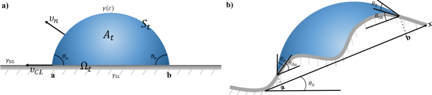
Figure 1. Illustration of surface tensions $\gamma_{\scriptscriptstyle{\text{SG}}},\gamma_{\scriptscriptstyle{\text{SL}}},\gamma(c)$ on three interfaces, contact angle $\theta_{\scriptscriptstyle{\text{CL}}}$, capillary surface $S_{t}$ and wetting domain $\Omega_{t}$ for droplets on a plane (left) or on an inclined substrate with an effective inclined angle $\theta_{0}$ (right).)

We regard the geometric states, i.e., the wetting domain $\Omega_{t}$ and the capillary surface $h(x,y,t)$ as a configuration of droplets. We assume the surfactant concentrates on the capillary surface, move with the evolutionary surface and may also has its own convention and diffusion on the surface. In the following subsections, we will first give some kinematic descriptions for the moving surface and the surfactant concentration on the capillary surface. Then we impose a boundary condition for the concentration of the surfactant $c$ on a prescribed moving capillary surface $h$ to preserve total mass and based on it we compute the rate of change of total surface energy; see Section 2.1. The rate of change of total energy $\dot{\mathcal{F}}$ in (3.26) quantifies the work done by the open system (capillary surface laid by surfactant and its contact line) against friction [16]. Then we only need to determine the velocity fields, including normal velocity of the capillary surface $v_{n}$ and contact line speed $v_{\scriptscriptstyle{\text{CL}}}$, via Onsager’s principle. In Section 2.2, from the energetic considerations, we introduce a specific Rayleigh dissipation functional and using Onsager’s principle to derive the contact line motion driven by the surfactant-dependent unbalanced Young force and finally the governing equations for the full dynamics of 3D droplets laid by the surfactant.

2.1. Kinematic descriptions for the moving surface, the surfactant concentration and energy

Surfactant dynamics on an evolutionary surface with the mass conservation law is a well-known model, c.f. [29]. For the case the surface has a graph representation $h(x,y,t),(x,y)\in\Omega_{t}$, we will provide a simple kinematic descriptions for the moving capillary surface, and the continuity equation for the concentration of the surfactant $c(x,y,t),(x,y)\in\Omega_{t}$ on the capillary surface. Based on this, the rate of change of the free energy $\mathcal{F}$ will then be calculated.

2.1.1. The continuity equation for the surfactant represented in the $xy$-plane

First, we describe the motion of the capillary surface $S_{t}$. Given a capillary surface with a graph representation $h(x,y,t),(x,y)\in\Omega_{t}$, any point on this moving capillary surface can be represented as

(2.7) $$X(t)=(x(t),y(t),h(x(t),y(t),t)).$$

Then the observed velocity of this point is

(2.8) $$\dot{X}=(\dot{x},\dot{y},h_{x}\dot{x}+h_{y}\dot{y}+h_{t}).$$

We assume there is an underlying velocity field $v\in\mathbb{R}^{3}$ driving the motion of the capillary surface, i.e.,

(2.9) $$\dot{X}(t)=v(X(t),t).$$

To clarify notations for functions of $(x,y)$ and functions of $(x,y,z)$, we introduce notations

(2.10) $$v(x,y,z,t)=:(v_{x},v_{y},v_{z})(x,y,z,t),$$

$$v(x,y,z,t)\big{|}_{z=h(x,y,t)}=:(v_{1},v_{2},v_{3})(x,y,t).$$

Using these notations, (2.9) implies the evolution of the surface in terms of $(x,y)\in\Omega_{t}$

(2.11) $$h_{t}+v_{1}h_{x}+v_{2}h_{y}=v_{3}.$$

Denote the normal vector as $n:=\frac{1}{\sqrt{1+|\nabla h|^{2}}}(-h_{x},-h_{y},1)$ and the tangential vectors as $\tau_{1}:=(1,0,h_{x}),\,\,\tau_{2}:=(0,1,h_{y})$. Then (2.11) becomes

(2.12) $$v_{n}:=v\cdot n=\frac{h_{t}}{\sqrt{1+|\nabla h|^{2}}}.$$

Now we express the velocity in the directions of the normal vector $n$ and the tangential vectors $\tau_{1},\,\tau_{2}$ as

(2.13) $$(v_{1},v_{2},v_{3})(x,y,t)=(v_{n}n+f\tau_{1}+g\tau_{2})(x,y,t),$$

where $\displaystyle f(x,y,t):=\frac{v\cdot\tau_{1}}{|\tau_{1}|^{2}},\,\,g(x,y,t):=\frac{v\cdot\tau_{2}}{|\tau_{2}|^{2}}$.

Second, we describe the dynamics of the concentration of the insoluble surfactant on the moving surface. Recall $\mathcal{C}(x,y,z,t),(x,y,z)\in S_{t}$ is the surface concentration of surfactant on the capillary surface and (2.2). Then using (2.11), we have

(2.14) $$\frac{\,\,\mathrm{d}}{\,\,\mathrm{d}t}\mathcal{C}(x(t),y(t),h(x(t),y(t),t),t)=(\partial_{t}+v\cdot\nabla)\mathcal{C}=(\partial_{t}+v_{1}\partial_{x}+v_{2}\partial_{y})c=\frac{\,\,\mathrm{d}}{\,\,\mathrm{d}t}c(x(t),y(t),t).$$

Therefore, the dynamics of the surfactant can be fully described by $c(x,y,t)$ on the $xy$-plane, as explained below.

We derive the continuity equation for $c(x,y,t),(x,y)\in\Omega_{t}.$ To do so, we use the $xy$-component of velocity $v$ to define a flow map on the $xy$-plane

(2.17) $$\left\{\begin{array}[]{cc}\dot{x}=v_{1}=v_{n}n_{1}+f=\frac{-h_{x}v_{n}}{\sqrt{1+|\nabla h|^{2}}}+f,\\ \dot{y}=v_{2}=v_{n}n_{2}+g=\frac{-h_{y}v_{n}}{\sqrt{1+|\nabla h|^{2}}}+g.\end{array}\right.$$

This flow map defines a 2D moving surface element $\omega_{t}\subset\Omega_{t}$ via $\omega_{t}=\{(x(t),y(t));(x_{0},y_{0})\in\omega_{0}\}$ with any given initial surface element $\omega_{0}$. In the absence of diffusion, $\omega_{t}$ can be regarded as a material element. That is to say, the mass in the material element $\omega_{t}$ is conserved

(2.18) $$\frac{\,\,\mathrm{d}}{\,\,\mathrm{d}t}\int_{\omega_{t}}c\sqrt{1+|\nabla h|^{2}}\,\,\mathrm{d}x\,\,\mathrm{d}y=0.$$

By (2.18) and the Reynolds transport theorem

(2.19) $$0=\frac{\,\,\mathrm{d}}{\,\,\mathrm{d}t}\int_{\omega_{t}}c\sqrt{1+|\nabla h|^{2}}\,\,\mathrm{d}x\,\,\mathrm{d}y=\int_{\omega_{t}}\partial_{t}\left(c\sqrt{1+|\nabla h|^{2}}\right)+\nabla\cdot\left(c\sqrt{1+|\nabla h|^{2}}\left(\begin{array}[]{c}v_{1}\\ v_{2}\end{array}\right)\right)\,\,\mathrm{d}x\,\,\mathrm{d}y.$$

Then by the arbitrary of $\omega_{t}$, the continuity equation for $c(x,y,t)$ is

(2.20) $$\partial_{t}\left(c\sqrt{1+|\nabla h|^{2}}\right)+\nabla\cdot\left(c\sqrt{1+|\nabla h|^{2}}\left(\begin{array}[]{c}v_{1}\\ v_{2}\end{array}\right)\right)=0\quad\text{ in }\Omega_{t}.$$

Plugging $v_{1},v_{2}$ defined in (2.17), we obtain the continuity equation for $c$

(2.21) $$0= (\partial_{t}c)\,{\sqrt{1+|\nabla h|^{2}}}+\frac{c}{\sqrt{1+|\nabla h|^{2}}}\nabla h\cdot\nabla h_{t}-\nabla\cdot\left(\frac{ch_{t}}{\sqrt{1+|\nabla h|^{2}}}\nabla h\right)+\nabla\cdot\left(c\sqrt{1+|\nabla h|^{2}}\left(\begin{array}[]{c}f\\ g\end{array}\right)\right)$$

$$= (\partial_{t}c)\,{\sqrt{1+|\nabla h|^{2}}}-h_{t}\nabla\cdot\left(\frac{c}{\sqrt{1+|\nabla h|^{2}}}\nabla h\right)+\nabla\cdot\left(c\sqrt{1+|\nabla h|^{2}}\left(\begin{array}[]{c}f\\ g\end{array}\right)\right)$$

After simplification, the continuity equation for $c$ is

(2.22) $$\partial_{t}c-v_{n}\nabla c\cdot\frac{\nabla h}{\sqrt{1+|\nabla h|^{2}}}+v_{n}cH+\frac{1}{{\sqrt{1+|\nabla h|^{2}}}}\nabla\cdot\left(c\sqrt{1+|\nabla h|^{2}}\left(\begin{array}[]{c}f\\ g\end{array}\right)\right)=0$$

for $(x,y)\in\Omega_{t}$, where $H:=-\nabla\cdot\left(\frac{\nabla h}{\sqrt{1+|\nabla h|^{2}}}\right)$ is the mean curvature.

2.1.2. Comparison with the lift-up dynamics of $\mathcal{C}$ on the capillary surface

We now compare the continuity equation (2.20) for $c(x,y,t)$ on $\Omega_{t}$ with the original 3D concentration $\mathcal{C}(x,y,z,t)$ on $S_{t}$. We have the following proposition on the equivalent formulation of the continuity equation in terms of $\mathcal{C}$ defined on the moving surface $S_{t}$. The proof of this proposition will be given in Appendix A.

Proposition 2.1.

The continuity equation (2.20) can be recast as

(2.23) $$(\partial_{t}+v\cdot\nabla)\mathcal{C}+\mathcal{C}\nabla_{s}\cdot v_{s}+v_{n}\mathcal{C}H=0\quad\text{ on }S_{t},$$

where $H=\nabla_{s}\cdot n$, $\nabla_{s}$ is the surface divergence and $v_{s}$ is the tangent velocity $v_{s}=v-(v\cdot n)n.$

Remark 1.

By some elementary calculations, we remark (2.23) is equivalent to [15, (2.13)] and also equivalent to [22, (2.10)]. Indeed, the tangential convection can be combined with the last two terms in (2.23) in a conservative form, i.e.,

(2.24) $$0= \partial_{t}\mathcal{C}+v_{n}n\cdot\nabla\mathcal{C}+v_{s}\cdot\nabla\mathcal{C}+\mathcal{C}\nabla_{s}\cdot v_{s}+v_{n}\mathcal{C}H$$

$$= \partial_{t}\mathcal{C}+v_{n}n\cdot\nabla\mathcal{C}+\nabla_{s}\cdot(\mathcal{C}v_{s})+v_{n}\mathcal{C}H$$

$$= \partial_{t}\mathcal{C}+v_{n}n\cdot\nabla\mathcal{C}+\nabla_{s}\cdot(\mathcal{C}v),\qquad\text{\cite[cite]{[\@@bibref{}{Garcke_Wieland_2006}{}{}, (2.13)]}}.$$

Notice also the last two terms can be combined together, so (2.23) is also equivalent to

(2.25) $$0= \partial_{t}\mathcal{C}+v\cdot\nabla\mathcal{C}+\mathcal{C}\nabla_{s}\cdot v_{s}+v_{n}\mathcal{C}H$$

$$= (\partial_{t}+v\cdot\nabla)\mathcal{C}+\mathcal{C}\nabla_{s}\cdot v,\qquad\text{\cite[cite]{[\@@bibref{}{Lai_2010}{}{}, (2.10)]}}.$$

We point out all these equivalent equations differ from ones presented in Stone [29, (6)], i.e.,

(2.26) $$\partial_{t}\mathcal{C}+\text{\sout{$v_{n}n\cdot\nabla\mathcal{C}$}}+\nabla_{s}\cdot(\mathcal{C}v_{s})+v_{n}\mathcal{C}H=0.$$

The second term above $v_{n}n\cdot\nabla\mathcal{C}$ vanishes only if concentration $\mathcal{C}$ has a constant normal extension outside the moving surface [1]. However, from Gurtin [19], $(\partial_{t}+v\cdot\nabla)$ is a tangential derivative of the space-time surface $\displaystyle\cup_{t\geq 0}S_{t}\times\{t\}$, so there is no need to extend $\mathcal{C}$ outside the space-time surface.

To describe the evolution of the capillary surface, we only need the normal velocity $v_{n}$ of the fluids. In the first special case, we consider the surfactant move with the evolving capillary surface, i.e., there is no additional tangential convection w.r.t. the capillary surface for the surfactant. We will call this special case, as “no free-slip” case. In this case, the continuity equation (2.22) can be completely described via $v_{n}$ and becomes

(2.27) $$\partial_{t}c-v_{n}\nabla\cdot\left(\frac{c}{\sqrt{1+|\nabla h|^{2}}}\nabla h\right)= \partial_{t}c-v_{n}\nabla c\cdot\frac{\nabla h}{\sqrt{1+|\nabla h|^{2}}}+v_{n}cH=0.$$

This formula is particularly efficient for simulating the purely geometric motion of the droplet and the surfactant is pinned to move with the capillary surface. For the general case that the continuity equation is completely described via $v$, one needs to consider the fluids inside the droplets instead of the purely geometric motion; see Section 3.

2.1.3. Diffusion of surfactant on the evolutionary surface

Furthermore, from some elementary calculations, the Dirichlet energy for the surfactant on the capillary surface is

(2.28) $$\frac{1}{2}\int_{S_{t}}|\nabla_{s}\mathcal{C}|^{2}\,\,\mathrm{d}s=\frac{1}{2}\int_{\Omega_{t}}\frac{1}{\sqrt{1+|\nabla h|^{2}}}\nabla c\cdot(M\nabla c)\,\,\mathrm{d}x\,\,\mathrm{d}y,$$

where $M:=I+\left(\begin{array}[]{c}-h_{y}\\ h_{x}\end{array}\right)\left(-h_{y},h_{x}\right)$. Then the variation of the Dirichlet energy gives the Laplace–Beltrami operator in the graph representation,

$$\Delta_{s}c:=\frac{1}{\sqrt{1+|\nabla h|^{2}}}\nabla\cdot\left(\frac{1}{\sqrt{1+|\nabla h|^{2}}}M\nabla c\right).$$

Thus in the “no free-slip” case, the continuity equation (2.27) for the surfactant with additional diffusion becomes

(2.29) $$c_{t}-\frac{h_{t}}{\sqrt{1+|\nabla h|^{2}}}\nabla\cdot\left(\frac{c\nabla h}{\sqrt{1+|\nabla h|^{2}}}\right)=D\Delta_{s}c,$$

which is equivalent to

(2.30) $$\partial_{t}c-v_{n}\nabla c\cdot\frac{\nabla h}{\sqrt{1+|\nabla h|^{2}}}+v_{n}cH=D\Delta_{s}c.$$

Here $D>0$ is a diffusion constant. This is the continuity equation with diffusion for the surfactant dynamics on the moving surface and we will impose the no-flux boundary condition for (2.29) below. Another equivalent form of (2.29) in the conservative form is

(2.31) $$\partial_{t}\left(c{\sqrt{1+|\nabla h|^{2}}}\right)-\nabla\cdot\left(\frac{ch_{t}}{\sqrt{1+|\nabla h|^{2}}}\nabla h\right)=D\nabla\cdot\left(\frac{1}{\sqrt{1+|\nabla h|^{2}}}M\nabla c\right).$$

2.1.4. The rate of change of the energy on the capillary surface

In this section, given an evolutionary capillary surface $h(x,y,t)$ and the associated surfactant dynamics (2.29) with (2.47), we calculate the rate of change of the energy for the capillary surface.

Consider the free energy on the capillary surface

(2.32) $$\mathcal{F}_{0}=\int_{\Omega_{t}}e(c)\sqrt{1+|\nabla h|^{2}}\,\,\mathrm{d}x\,\,\mathrm{d}y,$$

where $e(c)$ is the energy density on the capillary surface and $c(x,y,t)$ satisfies (2.29).

However, in calculations of the rate of change of the energy, the work done by the surface tension per unit time shall be a surfactant-dependent one, given by $\gamma(c)Hv_{n}$, where $\gamma(c)$ is the effective surface tension and $H=-\nabla\cdot\left(\frac{\nabla h}{\sqrt{1+|\nabla h|^{2}}}\right)$ is the mean curvature. We will derive this energy conservation law below.

First, the relation between the surfactant-dependent surface tension $\gamma(c)$ with the free energy density $e(c)$ is given by [8, 15]

(2.33) $$\gamma(c)=e(c)-e^{\prime}(c)c.$$

Indeed, from [8, (4.32)], $\gamma(c)=\gamma_{0}-\Pi_{A}(c)$. Here $\gamma_{0}=e(0)$ and $\Pi_{A}$ is the surface pressure which can be calculated by the osmotic pressure inside the interfacial layer due to the inhomogeneous surface concentration of surfactant. From the same derivations as [8, (2.23)],

$$\Pi_{A}(c)=-e(c)+e^{\prime}(c)c+e(0).$$

Thus we have (2.33).

Second, multiplying (2.30) by $e^{\prime}(c)\sqrt{1+|\nabla h|^{2}}$, we have

$$\left(\partial_{t}e(c)\right)\sqrt{1+|\nabla h|^{2}}-\nabla e(c)\cdot\frac{h_{t}\nabla h}{\sqrt{1+|\nabla h|^{2}}}+h_{t}He^{\prime}(c)c=D\sqrt{1+|\nabla h|^{2}}e^{\prime}(c)\Delta_{s}c.$$

We can recast this in the conservative form

(2.34) $$\partial_{t}\left(e(c)\sqrt{1+|\nabla h|^{2}}\right)-\nabla\cdot\left(e(c)\cdot\frac{h_{t}\nabla h}{\sqrt{1+|\nabla h|^{2}}}\right)+h_{t}He^{\prime}(c)c$$

$$\qquad\qquad-e(c)\partial_{t}\left(\sqrt{1+|\nabla h|^{2}}\right)+e(c)\nabla\cdot\left(\frac{h_{t}\nabla h}{\sqrt{1+|\nabla h|^{2}}}\right)=D\sqrt{1+|\nabla h|^{2}}e^{\prime}(c)\Delta_{s}c.$$

Then using the identity

(2.35) $$-\partial_{t}\left(\sqrt{1+|\nabla h|^{2}}\right)+\nabla\cdot\left(\frac{h_{t}\nabla h}{\sqrt{1+|\nabla h|^{2}}}\right)=-h_{t}H$$

and relation (2.33), we simplify (2.34) as

(2.36) $$\partial_{t}\left(e(c)\sqrt{1+|\nabla h|^{2}}\right)-\nabla\cdot\left(e(c)\cdot\frac{h_{t}\nabla h}{\sqrt{1+|\nabla h|^{2}}}\right)-\gamma(c)Hh_{t}=D\sqrt{1+|\nabla h|^{2}}e^{\prime}(c)\Delta_{s}c.$$

The first term in (2.36) is the rate of change of the energy density per unit time per unit area in the $xy$-plane. The second term in (2.36) is the flux of energy density. The third term in (2.36), i.e., $-\gamma(c)Hh_{t}=-\gamma(c)Hv_{n}\sqrt{1+|\nabla h|^{2}}$ is the rate of work done by the surface tension per unit area in the $xy$-plane. The last term in (2.36) is the energy density dissipation due to the diffusion of the surfactant.

Now we focus on our goal to derive the contact line dynamics which is driven by the effective surface tension $\gamma(c)$. However, notice the boundary condition can not be derived by taking trace of the interior velocity, so we will apply the Reynolds transport theorem using the boundary velocity of the moving domain. In the next subsection, we will discuss the correct boundary condition for the concentration of the surfactant.

The fundamental relation (2.33) implies the decreasing of $\gamma(c)$ from the convexity of energy density $e(c)$. Many interesting physical phenomena can be explained by the gradient of effective surface tension $\gamma(c)$ due to the gradient of surfactant concentration. For instance, the gradient of surface tension will drive the spreading of the droplet and the surfactant rapidly aggregates to the direction of lower concentration, which forms Marangoni flow on the surface. Particularly, when the concentration of surfactant is above a critical micelle value, the surfactant-driven spreading will lead to fingering phenomenon, an unstable structure on surfactant-laden droplets [4]. We remark a typical $\gamma$, derived from the Langmuir equation, is given by

(2.37) $$\gamma(c)=\gamma_{0}+c_{s}kT\ln(1-\frac{c}{c_{s}}),\quad e(c)=\gamma_{0}+kT\left((c_{s}-c)\ln(c_{s}-c)+c\ln c-c_{s}\ln c_{s}\right),$$

where $\gamma_{0}$ is the surface tension without the surfactant and $c_{s}$ is the saturated concentration [8]. We will demonstrate numerical examples using this typical $\gamma$.

2.1.5. Impose a boundary condition at the contact line for the surfactant to preserve total mass

To derive a boundary condition for the surfactant equation at the contact lines, we now apply the Reynolds transport theorem for the whole wetting domain $\Omega_{t}$ up to its boundary. We shall be careful when using the boundary velocity in the Reynolds transport theorem because the boundary condition of a PDE can not be derived by taking trace of the interior equation.

Denote $n_{\ell}$ as the outer normal of the contact line $\partial\Omega_{t}$ in the $xy$-plane and $v_{\ell}$ as the velocity of the contact line. We have $n_{\ell}=-\frac{\nabla h}{|\nabla h|}$ on the contact line $\partial\Omega_{t}$. Denote the normal speed of the contact line as $v_{\scriptscriptstyle{\text{CL}}}:=v_{\ell}\cdot n_{\ell}$. By the Reynolds transport theorem we have

(2.38) $$\frac{\,\,\mathrm{d}}{\,\,\mathrm{d}t}\int_{\Omega_{t}}c\sqrt{1+|\nabla h|^{2}}\,\,\mathrm{d}x\,\,\mathrm{d}y=\int_{\Omega_{t}}\partial_{t}\left(c\sqrt{1+|\nabla h|^{2}}\right)\,\,\mathrm{d}x\,\,\mathrm{d}y+\int_{\partial\Omega_{t}}c\sqrt{1+|\nabla h|^{2}}v_{\ell}\cdot n_{\ell}\,\,\mathrm{d}s.$$

Then by (2.31) and integration by parts, we obtain

(2.39) $$\int_{\Omega_{t}}\partial_{t}\left(c\sqrt{1+|\nabla h|^{2}}\right)\,\,\mathrm{d}x\,\,\mathrm{d}y=D\int_{\partial\Omega_{t}}\frac{1}{\sqrt{1+|\nabla h|^{2}}}M\nabla c\cdot n_{\ell}\,\,\mathrm{d}s+\int_{\partial\Omega_{t}}\frac{ch_{t}}{\sqrt{1+|\nabla h|^{2}}}\nabla h\cdot n_{\ell}\,\,\mathrm{d}s$$

Notice the definition of $M$ gives

(2.40) $$M\nabla c\cdot n_{\ell}=n_{\ell}\cdot\nabla c+n_{\ell}\cdot(-h_{y},h_{x})~{}(-h_{y},h_{x})\cdot\nabla c=n_{\ell}\cdot\nabla c\quad\text{ on }\partial\Omega_{t}.$$

Notice also the compatibility condition $\frac{\,\,\mathrm{d}h(x(t),y(t),t)}{\,\,\mathrm{d}t}=0$ on the contact line gives

(2.41) $$h_{t}=-\nabla h\cdot v_{\ell}.$$

Then from $n_{\ell}=-\frac{\nabla h}{|\nabla h|}$ on $\partial\Omega_{t}$, (2.41) becomes

(2.42) $$h_{t}=|\nabla h|n_{\ell}\cdot v_{\ell}=|\nabla h|v_{\scriptscriptstyle{\text{CL}}},$$

which implies

(2.43) $$\frac{h_{t}}{\sqrt{1+|\nabla h|^{2}}}\nabla h\cdot n_{\ell}=-\frac{|\nabla h|^{2}}{\sqrt{1+|\nabla h|^{2}}}v_{\scriptscriptstyle{\text{CL}}}.$$

Thus (2.39) can be further simplified as

(2.44) $$\int_{\Omega_{t}}\partial_{t}\left(c\sqrt{1+|\nabla h|^{2}}\right)\,\,\mathrm{d}x\,\,\mathrm{d}y=\int_{\partial\Omega_{t}}D\frac{n_{\ell}\cdot\nabla c}{\sqrt{1+|\nabla h|^{2}}}-c\frac{|\nabla h|^{2}}{\sqrt{1+|\nabla h|^{2}}}v_{\scriptscriptstyle{\text{CL}}}\,\,\mathrm{d}s.$$

Plugging this into (2.38), we have

(2.45) $$\frac{\,\,\mathrm{d}}{\,\,\mathrm{d}t}\int_{\Omega_{t}}c\sqrt{1+|\nabla h|^{2}}\,\,\mathrm{d}x\,\,\mathrm{d}y$$

$$= \int_{\partial\Omega_{t}}\frac{D}{\sqrt{1+|\nabla h|^{2}}}n_{\ell}\cdot\nabla c-\int_{\partial\Omega_{t}}c\frac{|\nabla h|^{2}}{\sqrt{1+|\nabla h|^{2}}}v_{\scriptscriptstyle{\text{CL}}}-c\sqrt{1+|\nabla h|^{2}}v_{\scriptscriptstyle{\text{CL}}}\,\,\mathrm{d}s$$

$$= \int_{\partial\Omega_{t}}\frac{D}{\sqrt{1+|\nabla h|^{2}}}n_{\ell}\cdot\nabla c+\int_{\partial\Omega_{t}}c\frac{1}{\sqrt{1+|\nabla h|^{2}}}v_{\scriptscriptstyle{\text{CL}}}\,\,\mathrm{d}s.$$

Therefore, in order to maintain the mass conservation law

(2.46) $$0=\frac{\,\,\mathrm{d}}{\,\,\mathrm{d}t}\int_{\Omega_{t}}c\sqrt{1+|\nabla h|^{2}}\,\,\mathrm{d}x\,\,\mathrm{d}y=\int_{\partial\Omega_{t}}\frac{1}{\sqrt{1+|\nabla h|^{2}}}\left(D\,n_{\ell}\cdot\nabla c+c\,v_{\scriptscriptstyle{\text{CL}}}\right)\,\,\mathrm{d}s,$$

we impose the following Robin boundary condition for (2.29)

(2.47) $$D\,n_{\ell}\cdot\nabla c+c\,v_{\scriptscriptstyle{\text{CL}}}=0\quad\text{ on }\partial\Omega_{t}.$$

2.1.6. Rate of change of the total surface energy

Using the Reynolds transport theorem for the surface energy

(2.48) $$\frac{\,\,\mathrm{d}}{\,\,\mathrm{d}t}\int_{\Omega_{t}}e(c)\sqrt{1+|\nabla h|^{2}}\,\,\mathrm{d}x\,\,\mathrm{d}y$$

$$= \int_{\Omega_{t}}\partial_{t}\left(e(c)\sqrt{1+|\nabla h|^{2}}\right)\,\,\mathrm{d}x\,\,\mathrm{d}y+\int_{\partial\Omega_{t}}e(c)\sqrt{1+|\nabla h|^{2}}v_{\scriptscriptstyle{\text{CL}}}\,\,\mathrm{d}s$$

$$= \int_{\Omega_{t}}\nabla\cdot\left(e(c)\cdot\frac{h_{t}\nabla h}{\sqrt{1+|\nabla h|^{2}}}\right)+\gamma(c)Hh_{t}+De^{\prime}(c)\nabla\cdot\left(\frac{1}{\sqrt{1+|\nabla h|^{2}}}M\nabla c\right)\,\,\mathrm{d}x\,\,\mathrm{d}y$$

$$+\int_{\partial\Omega_{t}}e(c)\sqrt{1+|\nabla h|^{2}}v_{\scriptscriptstyle{\text{CL}}}\,\,\mathrm{d}s,$$

where we used (2.36) in the last equality. Then using the integration by parts, (2.48) becomes

(2.49) $$\frac{\,\,\mathrm{d}}{\,\,\mathrm{d}t}\int_{\Omega_{t}}e(c)\sqrt{1+|\nabla h|^{2}}\,\,\mathrm{d}x\,\,\mathrm{d}y$$

$$= \int_{\Omega_{t}}h_{t}H\gamma(c)-D\frac{e^{\prime\prime}(c)}{\sqrt{1+|\nabla h|^{2}}}\nabla c\cdot M\nabla c\,\,\mathrm{d}x\,\,\mathrm{d}y$$

$$+\int_{\partial\Omega_{t}}e(c)\frac{h_{t}}{\sqrt{1+|\nabla h|^{2}}}\nabla h\cdot n_{\ell}+De^{\prime}(c)\frac{M\nabla c\cdot n_{\ell}}{\sqrt{1+|\nabla h|^{2}}}\,\,\mathrm{d}s +\int_{\partial\Omega_{t}}e(c)\sqrt{1+|\nabla h|^{2}}v_{\scriptscriptstyle{\text{CL}}}\,\,\mathrm{d}s.$$

Then using (2.43) and (2.40), by the same calculations as (2.45), we have

(2.50) $$\frac{\,\,\mathrm{d}}{\,\,\mathrm{d}t}\int_{\Omega_{t}}e(c)\sqrt{1+|\nabla h|^{2}}\,\,\mathrm{d}x\,\,\mathrm{d}y$$

$$= \int_{\Omega_{t}}h_{t}\gamma(c)H-D\frac{e^{\prime\prime}(c)}{\sqrt{1+|\nabla h|^{2}}}\nabla c\cdot M\nabla c\,\,\mathrm{d}x\,\,\mathrm{d}y +\int_{\partial\Omega_{t}}\frac{1}{\sqrt{1+|\nabla h|^{2}}}[De^{\prime}(c)\,n_{\ell}\cdot\nabla c+e(c)v_{\scriptscriptstyle{\text{CL}}}]\,\,\mathrm{d}s,$$

From the boundary condition (2.47), we have

(2.51) $$De^{\prime}(c)\,n_{\ell}\cdot\nabla c+e(c)v_{\scriptscriptstyle{\text{CL}}}=-e^{\prime}(c)c\,v_{\scriptscriptstyle{\text{CL}}}+e(c)v_{\scriptscriptstyle{\text{CL}}}=\gamma(c)v_{\scriptscriptstyle{\text{CL}}}.$$

Thus, this, together with (2.50), implies the rate of change of the surface energy $\mathcal{F}_{0}$

(2.52) $$\frac{\,\,\mathrm{d}}{\,\,\mathrm{d}t}\int_{\Omega_{t}}e(c)\sqrt{1+|\nabla h|^{2}}\,\,\mathrm{d}x\,\,\mathrm{d}y$$

$$= \int_{\Omega_{t}}\gamma(c)h_{t}H-D\frac{e^{\prime\prime}(c)}{\sqrt{1+|\nabla h|^{2}}}\nabla c\cdot M\nabla c\,\,\mathrm{d}x\,\,\mathrm{d}y+\int_{\partial\Omega_{t}}\gamma(c)\cos\theta_{\scriptscriptstyle{\text{CL}}}\,v_{\scriptscriptstyle{\text{CL}}}\,\,\mathrm{d}s,$$

where we used $\cos\theta_{\scriptscriptstyle{\text{CL}}}=\frac{1}{\sqrt{1+|\nabla h|^{2}}}$ on $\partial\Omega_{t}$.

From (2.52) and the rate of change of the surface energy for the bottom part

$$\frac{\,\,\mathrm{d}}{\,\,\mathrm{d}t}(\gamma_{\scriptscriptstyle{\text{SL}}}-\gamma_{\scriptscriptstyle{\text{SG}}})\int_{\Omega_{t}}\,\,\mathrm{d}x\,\,\mathrm{d}y=(\gamma_{\scriptscriptstyle{\text{SL}}}-\gamma_{\scriptscriptstyle{\text{SG}}})\int_{\partial\Omega_{t}}v_{\scriptscriptstyle{\text{CL}}}\,\,\mathrm{d}s,$$

we finally obtain the rate of change of the total surface energy

(2.53) $$\frac{\,\,\mathrm{d}}{\,\,\mathrm{d}t}\left(\int_{\Omega_{t}}e(c)\sqrt{1+|\nabla h|^{2}}\,\,\mathrm{d}x\,\,\mathrm{d}y+(\gamma_{\scriptscriptstyle{\text{SL}}}-\gamma_{\scriptscriptstyle{\text{SG}}})\int_{\Omega_{t}}\,\,\mathrm{d}x\,\,\mathrm{d}y\right)$$

$$= \int_{\Omega_{t}}\gamma(c)h_{t}H-D\frac{e^{\prime\prime}(c)}{\sqrt{1+|\nabla h|^{2}}}\nabla c\cdot M\nabla c\,\,\mathrm{d}x\,\,\mathrm{d}y+\int_{\partial\Omega_{t}}\left(\gamma(c)\cos\theta_{\scriptscriptstyle{\text{CL}}}+\gamma_{\scriptscriptstyle{\text{SL}}}-\gamma_{\scriptscriptstyle{\text{SG}}}\right)v_{\scriptscriptstyle{\text{CL}}}\,\,\mathrm{d}s.$$

With the volume constraint $V$, we take the total free energy of the droplet as

(2.54) $$\mathcal{F}(h(t),\Omega_{t},\lambda(t))=\int_{\Omega_{t}}e(c)\sqrt{1+|\nabla u|^{2}}\,\,\mathrm{d}x\,\,\mathrm{d}y+(\gamma_{\scriptscriptstyle{\text{SL}}}-\gamma_{\scriptscriptstyle{\text{SG}}})\int_{\Omega_{t}}\,\,\mathrm{d}x\,\,\mathrm{d}y-\lambda(t)\left(\int_{\Omega_{t}}h\,\,\mathrm{d}x\,\,\mathrm{d}y-V\right),$$

where $\lambda(t)$ is a Lagrangian multiplier. Thus, given $h(x,y,t)$ and $c(c,y,t)$, the rate of change of the total free energy can be regarded as a functional of $h_{t},v_{\scriptscriptstyle{\text{CL}}}$. Denote

(2.55) $$\frac{\,\,\mathrm{d}}{\,\,\mathrm{d}t}\mathcal{F}(h_{t},v_{\scriptscriptstyle{\text{CL}}};h,c):=\frac{\,\,\mathrm{d}}{\,\,\mathrm{d}t}\mathcal{F}= -\int_{\Omega_{t}}\left(-\gamma(c)H+\lambda\right)h_{t}\,\,\mathrm{d}x\,\,\mathrm{d}y-D\int_{\Omega_{t}}\frac{e^{\prime\prime}(c)}{\sqrt{1+|\nabla h|^{2}}}\nabla c\cdot M\nabla c\,\,\mathrm{d}x\,\,\mathrm{d}y$$

$$+\int_{\partial\Omega_{t}}\left(\gamma(c)\cos\theta_{\scriptscriptstyle{\text{CL}}}+(\gamma_{\scriptscriptstyle{\text{SL}}}-\gamma_{\scriptscriptstyle{\text{SG}}})\right)v_{\scriptscriptstyle{\text{CL}}}\,\,\mathrm{d}s.$$

The derivation with some additional potential forces is standard and will not be included here.

2.2. The Onsager principle and the governing equations in 3D

In Section 2.1, we used the normal velocity $v_{n}$ and the contact line speed $v_{\scriptscriptstyle{\text{CL}}}$ to give kinematic descriptions including (i) the motion of the capilary surface (2.12), (ii) the continuity equation of the surfactant (2.30) and (iii) the rate of change of total energy (2.55). Now we determine these velocities $v_{n},v_{\scriptscriptstyle{\text{CL}}}$ from energetic considerations via Onsager’s principle.

From energetic considerations, we choose the following Rayleigh dissipation functional

(2.56) $$Q(h_{t},v_{\scriptscriptstyle{\text{CL}}};h,c):=\frac{\beta}{2}\int_{\Omega_{t}}\frac{h_{t}^{2}}{\sqrt{1+|\nabla h|^{2}}}\,\,\mathrm{d}x\,\,\mathrm{d}y+\frac{\xi}{2}\int_{\partial\Omega_{t}}|v_{\scriptscriptstyle{\text{CL}}}|^{2}\,\,\mathrm{d}s+\frac{D}{2}\int_{\Omega_{t}}\frac{e^{\prime\prime}(c)}{\sqrt{1+|\nabla h|^{2}}}\nabla c\cdot M\nabla c\,\,\mathrm{d}x\,\,\mathrm{d}y,$$

where $\beta$ represents the friction coefficient for the normal motion of the capillary surface, $\xi$ represents the friction coefficient for the moving contact lines and the last term represents the dissipation due to the diffusion of the surfactant. We will see the first term in (2.56) leads to the motion by mean curvature of the capillary surface [17]. Then minimizing the Rayleighian [8]

(2.57) $$\mathcal{R}(h_{t},v_{\scriptscriptstyle{\text{CL}}};h,c):=Q(h_{t},v_{\scriptscriptstyle{\text{CL}}};h,c)+\frac{\,\,\mathrm{d}}{\,\,\mathrm{d}t}\mathcal{F}(h_{t},v_{\scriptscriptstyle{\text{CL}}};h,c)$$

with respect to $(h_{t},v_{\scriptscriptstyle{\text{CL}}})$ gives the governing equation

(2.58) $$\frac{\beta}{\sqrt{1+|\nabla h|^{2}}}h_{t}=-\gamma(c)H+\lambda,$$

$$\xi v_{\scriptscriptstyle{\text{CL}}}=-\gamma(c)\cos\theta_{\scriptscriptstyle{\text{CL}}}-(\gamma_{\scriptscriptstyle{\text{SL}}}-\gamma_{\scriptscriptstyle{\text{SG}}}),$$

where the right hand side $F_{s}=-\gamma(c)\cos\theta_{\scriptscriptstyle{\text{CL}}}-(\gamma_{\scriptscriptstyle{\text{SL}}}-\gamma_{\scriptscriptstyle{\text{SG}}})$ is exactly the surfactant-dependent unbalanced Young force.

Combining this with (2.29), the full system is

(2.59) $$\left\{\begin{aligned} &\frac{\beta}{\sqrt{1+|\nabla h|^{2}}}h_{t}=-\gamma(c)H+\lambda,\quad h(x,y)|_{\partial\Omega_{t}}=0,\\ &c_{t}-\frac{h_{t}}{\sqrt{1+|\nabla h|^{2}}}\nabla\cdot\left(\frac{c\nabla h}{\sqrt{1+|\nabla h|^{2}}}\right)=D\Delta_{s}c,\quad cv_{\scriptscriptstyle{\text{CL}}}+D\,n_{\ell}\cdot\nabla c\big{|}_{\partial\Omega_{t}}=0,\\ &\xi v_{\scriptscriptstyle{\text{CL}}}=-\gamma(c)\cos\theta_{\scriptscriptstyle{\text{CL}}}-(\gamma_{\scriptscriptstyle{\text{SL}}}-\gamma_{\scriptscriptstyle{\text{SG}}}),\quad\text{ on }\partial\Omega_{t},\\ &\int_{\Omega_{t}}h\,\,\mathrm{d}x\,\,\mathrm{d}y=V.\end{aligned}\right.$$

This system can be regarded as (i) the linear response relation of $v_{n}$ to the Laplace pressure $\gamma(c)H$, (ii) the linear response relation of $v_{\scriptscriptstyle{\text{CL}}}$ to the surfactant-dependent unbalanced Young force $F_{s}$, and (iii) the transport of the insoluble surfactant on the capillary surface.

As a consequence, the energy dissipation relation is

(2.60) $$\frac{\,\,\mathrm{d}}{\,\,\mathrm{d}t}\mathcal{F}= -\int_{\Omega_{t}}\frac{\beta h_{t}^{2}}{\sqrt{1+|\nabla h|^{2}}}\,\,\mathrm{d}x\,\,\mathrm{d}y-D\int_{\Omega_{t}}\frac{e^{\prime\prime}(c)}{\sqrt{1+|\nabla h|^{2}}}\nabla c\cdot M\nabla c\,\,\mathrm{d}x\,\,\mathrm{d}y-\int_{\partial\Omega_{t}}\xi|v_{\scriptscriptstyle{\text{CL}}}|^{2}\,\,\mathrm{d}s$$

$$= -2Q.$$

In physics, $\frac{2Q}{T}$ is denoted as $\dot{S}$, the entropy production rate.

We point out that the first dissipation term in Rayleigh dissipation functional (2.56) is not a standard one. Instead, the standard dissipation functional includes the dissipation due to the viscosity of fluids inside the droplet, for which we will also give a simple derivation using Onsager’s principle in Section 3. However, our choice of the Rayleigh dissipation functional (2.56) allows us to study the purely geometric motion of the droplets and has the following advantages. (i) For small droplets, it captures the essential physics and the leading behaviors of the droplet dynamics; (ii) it satisfies the Onsager principle in physics and thus has a gradient flow structure so that this simplified model is friendly for theoretical studies; (iii) this model is also computationally efficient because it does not need to compute the fluids inside the droplets and the numerical schemes can be easily adapt to more complicated physical examples such as inclined textured substrates, the electrowetting and the surfactant dynamics considered here.

3. Surfactant-induced Marangoni stress and viscous flow

In this section, we derive the surfactant-induced Marangoni flow for droplets on a substrate by including the viscous bulk fluids inside the droplets. Including the fluid viscosity dissipation in the Rayleigh dissipation functional, instead of the first term in (2.56), will lead to the Stokes equations for fluids inside droplets [20, 34, 21] or the thin film equation in the lubrication approximation [21, 33]. Although different forms of viscous flow models coupled with moving contact lines and surfactant transport were derived previously, we adapt the energy law on the capillary surface (2.36) to the general case, i.e., the surfactant moves on the capillary surface along with both the normal velocity $v_{n}$ and tangential velocity $v_{s}$ of the fluids, and then use Onsager’s principle to give a simple derivation for the viscous bulk fluids inside the droplet coupled with the Marangoni flow induced by the surfactant. We will see in (3.21) and (3.29) that the variation of the total surface energy with a surfactant-dependent surface tension will exerts an additional force $\nabla_{s}\gamma(c)$ for the bulk fluids at the capillary surface $S_{t}$. This surface gradient of the effective surface tension induces a Marangoni flow, and thus this phenomena is called Marangoni effect. At the end of this section, we also point out the two cases with or without bulk fluids inside the droplet are indeed quite similar in terms of the linear response relation $u=\mathcal{K}F$; see (3.39). In Proposition 3.1, we will prove the Rayleigh dissipation functional for the viscous flow case is indeed stronger than the one for the motion by mean curvature of the capillary surface. However, the bulk fluids cases with both the hydrodynamic effect of the viscous bulk fluids inside the droplet and the surfactant effect on the moving surface, i.e., the case that the dynamics of the bulk fluids is described by the Stokes equation coupled with the advection-diffusion of the surfactant on the moving capillary surface (see (3.29)), require additional computations for bulk fluids. Thus the computational strategies presented in Section 4 shall be modified and will be left as a future research.

Now let us first state the idea of derivations for the governing equations (3.29) for the general “free-slip” case, i.e., the surfactant moves on the capillary surface along with both the normal velocity $v_{n}$ and tangential velocity $v_{s}$ of the fluids inside the droplet. For this general case, given an underlying velocity $v$, the kinematic description for the capillary surface is still (2.11), i.e., $h_{t}+v_{1}h_{x}+v_{2}h_{y}=v_{3}$, and the continuity equation for the surfactant becomes (3.1). Below, we will follow the procedures in Section 2 to first give the kinematic descriptions for the rate of change of total energy in Section 3.1. After the calculations for the rate of change of total energy $\dot{\mathcal{F}}$ in (3.26), it quantifies the work done by the open system (capillary surface laid by surfactant and its contact line) against friction [16]. Then we determine the velocity fields, including fluid velocity $v$ and contact line speed $v_{\scriptscriptstyle{\text{CL}}}$, via energy considerations in Section 3.2, i.e., via Onsager’s principle by introducing a new Rayleigh dissipation functional $Q$. These immediately yield the governing equations and the energy dissipation law for the bulk fluids coupled with transport of surfactant on the evolutionary surface; see (3.29). In the end of this section, we give a proof of Onsager’s reciprocal relation and obtain a lower bound estimate for energy dissipation in Proposition 3.1, which helps us to characterize the steady solution as a spherical cap laid by constant-concentrated surfactant.

3.1. Kinematic descriptions for the rate of change of total energy

In the following subsections, we will adapt the same kinematic descriptions as in Section 2 to the general “free-slip” case for surfactant with $v_{s}$, derive the corresponding boundary conditions of the surfactant at the contact line and compute the rate of change of the total surface energy. With the convection contribution, transport equation (2.31) for $c$ becomes

(3.1) $$\partial_{t}\left(c{\sqrt{1+|\nabla h|^{2}}}\right)-\nabla\cdot\left(\frac{ch_{t}}{\sqrt{1+|\nabla h|^{2}}}\nabla h\right)+\nabla\cdot\left(c\sqrt{1+|\nabla h|^{2}}\left(\begin{array}[]{c}f\\ g\end{array}\right)\right)=D\nabla\cdot\left(\frac{1}{\sqrt{1+|\nabla h|^{2}}}M\nabla c\right).$$

We impose a non-flux boundary condition

(3.2) $$n_{\ell}\cdot\nabla c\big{|}_{\partial\Omega_{t}}=0$$

for $c$ to preserve the total mass of the surfactant.

3.1.1. Conservation of the total mass of the surfactant

Using (3.1) and the same calculus derivations as (2.45) except for adding $(f,g)$, we have

(3.3) $$\frac{\,\,\mathrm{d}}{\,\,\mathrm{d}t}\int_{\Omega_{t}}c\sqrt{1+|\nabla h|^{2}}\,\,\mathrm{d}x\,\,\mathrm{d}y$$

$$= \int_{\partial\Omega_{t}}\frac{D}{\sqrt{1+|\nabla h|^{2}}}n_{\ell}\cdot\nabla c+\int_{\partial\Omega_{t}}c\frac{1}{\sqrt{1+|\nabla h|^{2}}}v_{\scriptscriptstyle{\text{CL}}}-c\sqrt{1+|\nabla h|^{2}}\left(\begin{array}[]{c}f\\ g\end{array}\right)\cdot n_{\ell}\,\,\mathrm{d}s.$$

The first term on the right-hand-side vanishes due to the no-flux boundary condition (3.2). Recall (2.13). Suppose we impose the non-penetration boundary condition for the bulk fluid velocity $v\cdot e_{z}|_{\partial\Omega_{t}}=0$. Then

(3.4) $$v\cdot e_{z}=\frac{v_{n}}{\sqrt{1+|\nabla h|^{2}}}+h_{x}f+h_{y}g=0\quad\text{ on }\partial\Omega_{t}.$$

Then by $n_{\ell}=-\frac{\nabla h}{|\nabla h|}$, we have

(3.5) $$\frac{v_{n}}{\sqrt{1+|\nabla h|^{2}}}=|\nabla h|\left(\begin{array}[]{c}f\\ g\end{array}\right)\cdot n_{\ell}.$$

From this and the continuity condition (2.42), we know the last two terms in (3.3) also vanish

(3.6) $$\frac{1}{\sqrt{1+|\nabla h|^{2}}}v_{\scriptscriptstyle{\text{CL}}}-\sqrt{1+|\nabla h|^{2}}\left(\begin{array}[]{c}f\\ g\end{array}\right)\cdot n_{\ell}=0.$$

Hence (3.3) yields $\frac{\,\,\mathrm{d}}{\,\,\mathrm{d}t}\int_{\Omega_{t}}c\sqrt{1+|\nabla h|^{2}}\,\,\mathrm{d}x\,\,\mathrm{d}y=0.$

3.1.2. Calculations of Marangoni stress induced by the tangential convection of surfactant

Recall $(v_{1},v_{2})(x,y,t)$ is the $xy$-component of the velocity of the moving capillary surface. Then (3.1) is recast as

(3.7) $$\partial_{t}\left(c{\sqrt{1+|\nabla h|^{2}}}\right)+\nabla\cdot\left(c\sqrt{1+|\nabla h|^{2}}\left(\begin{array}[]{c}v_{1}\\ v_{2}\end{array}\right)\right)=D\nabla\cdot\left(\frac{1}{\sqrt{1+|\nabla h|^{2}}}M\nabla c\right).$$

Then by same calculations as (2.36), we obtain the change of the surface energy

(3.8) $$\partial_{t}\left(e(c){\sqrt{1+|\nabla h|^{2}}}\right)+\nabla\cdot\left(e(c)\sqrt{1+|\nabla h|^{2}}\left(\begin{array}[]{c}v_{1}\\ v_{2}\end{array}\right)\right)$$

$$= \gamma(c)\left(\partial_{t}{\sqrt{1+|\nabla h|^{2}}}+\nabla\cdot\left(\sqrt{1+|\nabla h|^{2}}\left(\begin{array}[]{c}v_{1}\\ v_{2}\end{array}\right)\right)\right)+D\sqrt{1+|\nabla h|^{2}}e^{\prime}(c)\Delta_{s}c$$

$$=: \gamma(c)I+D\sqrt{1+|\nabla h|^{2}}e^{\prime}(c)\Delta_{s}c.$$

Here using the identity (2.35), $\gamma(c)I$ can be further simplified as

(3.13) $$\gamma(c)I= \gamma(c)h_{t}H-\nabla\gamma(c)\cdot\left(\sqrt{1+|\nabla h|^{2}}\left(\begin{array}[]{c}f\\ g\end{array}\right)\right)+\nabla\cdot\left(\gamma(c)\sqrt{1+|\nabla h|^{2}}\left(\begin{array}[]{c}f\\ g\end{array}\right)\right)$$

(3.18) $$= -\sqrt{1+|\nabla h|^{2}}\left(-\gamma(c)v_{n}H+\left(\begin{array}[]{c}f\\ g\end{array}\right)\cdot\nabla\gamma(c)\right)+\nabla\cdot\left(\gamma(c)\sqrt{1+|\nabla h|^{2}}\left(\begin{array}[]{c}f\\ g\end{array}\right)\right).$$

Now we simplify the first term in $\gamma(c)I$ to see that besides the Laplace pressure, there is an additional force, brought by the surface gradient of $\gamma(\mathcal{C})$. Recall $v=v_{n}n+v_{s}.$ Denote

(3.19) $$F:=-\gamma(c)Hn+\nabla_{s}\gamma(\mathcal{C}).$$

Here the additional force term, surface gradient $\nabla_{s}\gamma(\mathcal{C})$, is called the Marangoni stress, so the total capillary force density $F$ exerting to the environment consists of both the negative Laplace pressure done by the capillary surface and the Marangoni stress caused by the surface gradient of surfactant-dependent surface tension. We now prove the first term in $\gamma(c)I$ satisfies

(3.20) $$-\gamma(c)v_{n}H+\left(\begin{array}[]{c}f\\ g\end{array}\right)\cdot\nabla_{xy}\gamma(c)=v\cdot F.$$

In other words, the first term in (3.18) can be recast as the work done by the capillary surface per unit time $v\cdot F$. Indeed, from the orthogonality and definition of $F$ in (3.19), we have

(3.21) $$v\cdot F=-v_{n}\gamma(c)H+v_{s}\cdot\nabla_{s}\gamma(\mathcal{C})\quad\text{ on }z=h(x,y,t).$$

By the definition of $v_{s}$ and surface gradient, the last term is

$$v_{s}\cdot\nabla_{s}\gamma(\mathcal{C})= (f\tau_{1}+g\tau_{2})\cdot[(I-n\otimes n)\nabla\gamma(\mathcal{C})]$$

$$= (f\tau_{1}+g\tau_{2})\cdot\nabla\gamma(\mathcal{C})=\left(\begin{array}[]{c}f\\ g\end{array}\right)\cdot\nabla_{xy}\gamma(c).$$

3.1.3. Rate of change of total surface energy

Recall the calculations for energy change (3.8) and its relation with the Marangoni stress $F$ in (3.20). Using the same calculations as (2.49), we can simplify the second term in (3.18)

(3.22) $$\frac{\,\,\mathrm{d}}{\,\,\mathrm{d}t}\int_{\Omega_{t}}e(c)\sqrt{1+|\nabla h|^{2}}\,\,\mathrm{d}x\,\,\mathrm{d}y$$

$$= -\int_{\Omega_{t}}v\cdot F\sqrt{1+|\nabla h|^{2}}\,\,\mathrm{d}x\,\,\mathrm{d}y-\int_{\Omega_{t}}D\frac{e^{\prime\prime}(c)}{\sqrt{1+|\nabla h|^{2}}}\nabla c\cdot M\nabla c\,\,\mathrm{d}x\,\,\mathrm{d}y$$

$$+\int_{\partial\Omega_{t}}e(c)\frac{h_{t}}{\sqrt{1+|\nabla h|^{2}}}\nabla h\cdot n_{\ell}-ce^{\prime}(c)\sqrt{1+|\nabla h|^{2}}\left(\begin{array}[]{c}f\\ g\end{array}\right)\cdot n_{\ell}\,\,\mathrm{d}s+\int_{\partial\Omega_{t}}e(c)\sqrt{1+|\nabla h|^{2}}v_{\scriptscriptstyle{\text{CL}}}\,\,\mathrm{d}s,$$

where we used the no-flux boundary condition (3.2). Using (3.6) and (2.43),

(3.23) $$\frac{\,\,\mathrm{d}}{\,\,\mathrm{d}t}\int_{\Omega_{t}}e(c)\sqrt{1+|\nabla h|^{2}}\,\,\mathrm{d}x\,\,\mathrm{d}y$$

$$= -\int_{\Omega_{t}}v\cdot F\sqrt{1+|\nabla h|^{2}}\,\,\mathrm{d}x\,\,\mathrm{d}y-\int_{\Omega_{t}}D\frac{e^{\prime\prime}(c)}{\sqrt{1+|\nabla h|^{2}}}\nabla c\cdot M\nabla c\,\,\mathrm{d}x\,\,\mathrm{d}y$$

$$+\int_{\partial\Omega_{t}}-e(c)\frac{|\nabla h|^{2}}{\sqrt{1+|\nabla h|^{2}}}v_{\scriptscriptstyle{\text{CL}}}-ce^{\prime}(c)\frac{1}{\sqrt{1+|\nabla h|^{2}}}v_{\scriptscriptstyle{\text{CL}}}\,\,\mathrm{d}s+\int_{\partial\Omega_{t}}e(c)\sqrt{1+|\nabla h|^{2}}v_{\scriptscriptstyle{\text{CL}}}\,\,\mathrm{d}s$$

$$= -\int_{\Omega_{t}}v\cdot F\sqrt{1+|\nabla h|^{2}}\,\,\mathrm{d}x\,\,\mathrm{d}y-\int_{\Omega_{t}}D\frac{e^{\prime\prime}(c)}{\sqrt{1+|\nabla h|^{2}}}\nabla c\cdot M\nabla c\,\,\mathrm{d}x\,\,\mathrm{d}y+\int_{\partial\Omega_{t}}\gamma(c)v_{\scriptscriptstyle{\text{CL}}}\frac{1}{\sqrt{1+|\nabla h|^{2}}}\,\,\mathrm{d}s.$$

Therefore in the presence of convention contribution of surfactant, the rate of change of the total surface energy becomes

(3.24) $$\frac{\,\,\mathrm{d}}{\,\,\mathrm{d}t}\Big{[}\int_{\Omega_{t}}e(c)\sqrt{1+|\nabla h|^{2}}\,\,\mathrm{d}x\,\,\mathrm{d}y+(\gamma_{\scriptscriptstyle{\text{SL}}}-\gamma_{\scriptscriptstyle{\text{SG}}})\int_{\Omega_{t}}\,\,\mathrm{d}x\,\,\mathrm{d}y\Big{]}$$

$$= -\int_{\Omega_{t}}v\cdot F\sqrt{1+|\nabla h|^{2}}\,\,\mathrm{d}x\,\,\mathrm{d}y-\int_{\Omega_{t}}D\frac{e^{\prime\prime}(c)}{\sqrt{1+|\nabla h|^{2}}}\nabla c\cdot M\nabla c\,\,\mathrm{d}x\,\,\mathrm{d}y-\int_{\partial\Omega_{t}}F_{s}v_{\scriptscriptstyle{\text{CL}}}\,\,\mathrm{d}s,$$

where $F_{s}=-\gamma(c)\cos\theta_{\scriptscriptstyle{\text{CL}}}+\gamma_{\scriptscriptstyle{\text{SG}}}-\gamma_{\scriptscriptstyle{\text{SL}}}$ is the surfactant-dependent unbalanced Young force.

3.2. Energetic descriptions: Stokes flow for bulk fluids and governing equations derived by Onsager’s principle

As we used the fluid velocity $v$ and the contact line speed $v_{\scriptscriptstyle{\text{CL}}}$ to give kinematic descriptions including motion of the capilary surface, the continuity equation of the surfactant and the rate of change of total energy (3.24), it remains to determine these velocities $v,v_{\scriptscriptstyle{\text{CL}}}$ from energetic considerations. Using Onsager’s principle and a new Rayleigh dissipation functional, we give derivations for the governing equations of the surfactant induced Marangoni flow coupled with moving contact lines.

Let $u(x,y,z,t)$ be the velocity of the bulk fluids. Assume the velocity $v$ of the capillary surface coincides with the velocity $u$ of the bulk fluids restricted on the capillary surface, i.e., $v(x,y,t)=u(x,y,z,t)\big{|}_{z=h(x,y,t)}$.

First, we impose the non-penetration boundary condition for the bottom of the droplet

(3.25) $$u\cdot n=0\quad\text{ on }\Omega_{t}$$

and consider an incompressible fluid satisfying $\nabla\cdot u=0$ inside the droplet $A_{t}$.

Given $h(x,y,t)$ and $c(x,y,t)$, then the rate of change of the total surface energy (3.24) can be regarded as a linear functional of $u,v_{\scriptscriptstyle{\text{CL}}}$ and we denote it as

(3.26) $$\dot{\mathcal{F}}(u,v_{\scriptscriptstyle{\text{CL}}};h,c):=-\int_{\Omega_{t}}u\cdot F\sqrt{1+|\nabla h|^{2}}\,\,\mathrm{d}x\,\,\mathrm{d}y-\int_{\Omega_{t}}D\frac{e^{\prime\prime}(c)}{\sqrt{1+|\nabla h|^{2}}}\nabla c\cdot M\nabla c\,\,\mathrm{d}x\,\,\mathrm{d}y-\int_{\partial\Omega_{t}}F_{s}v_{\scriptscriptstyle{\text{CL}}}\,\,\mathrm{d}s.$$

We remark the rate of change of total energy $\dot{\mathcal{F}}$ in (3.26) quantifies the work done by the open system (capillary surface laid by surfactant and its contact line) against friction [16]. Then all we need to do is to determine the the fluid velocity $u$ and the contact line speed $v_{\scriptscriptstyle{\text{CL}}}$ via Onsager’s principle by introducing a proper Rayleigh dissipation functional $Q$. In general, the choice of the Rayleigh dissipation functional in Onsager’s principle is just from phenomenological modeling instead of from physical principle. Therefore, Onsager’s principle is valid only for certain class of problems. However, many specific problems in soft matter including diffusion, viscous fluids and surfactant belong to this class. The resulting governing equations determined by the choice of Rayleighian are consistent with some well-accepted or experimentally tested models, for instance, the Navier-Stokes equations and the stokes equations in the current section; see more worked out examples in Doi’s book [9].

Second, given $h(x,y,t)$ and $c(x,y,t)$, introduce the Rayleigh dissipation functional $Q$

(3.27) $$Q(u,v_{\scriptscriptstyle{\text{CL}}};h,c):=\frac{\mu}{4}\int_{A_{t}}(\nabla u+\nabla u^{\top}):(\nabla u+\nabla u^{\top})\,\,\mathrm{d}V +\frac{D}{2}\int_{\Omega_{t}}\frac{e^{\prime\prime}(c)}{\sqrt{1+|\nabla h|^{2}}}\nabla c\cdot M\nabla c\,\,\mathrm{d}x\,\,\mathrm{d}y$$

$$+\frac{\mu}{2\alpha}\int_{\Omega_{t}}u^{2}\,\,\mathrm{d}x\,\,\mathrm{d}y+\frac{\xi}{2}\int_{\partial\Omega_{t}}|v_{\scriptscriptstyle{\text{CL}}}|^{2}\,\,\mathrm{d}s,$$

where $\mu$ is the dynamics viscosity for the bulk fluids and $\alpha$ is the slip length.

Given $h(x,y,t)$ and $c(x,y,t)$, define Rayleighnian as

(3.28) $$\mathcal{R}(u,v_{\scriptscriptstyle{\text{CL}}};h,c):=Q(u,v_{\scriptscriptstyle{\text{CL}}};h,c)+\dot{\mathcal{F}}(u,v_{\scriptscriptstyle{\text{CL}}};h,c).$$

Then based on Onsager’s principle, we minimize $\mathcal{R}(u,v_{\scriptscriptstyle{\text{CL}}};h,c)$ w.r.t the velocity $u,v_{\scriptscriptstyle{\text{CL}}}$. This yields the following governing equations, whose derivations are given in three steps below.

After incorporating the transport equation (3.1) for surfactant $c$ and the no-flux boundary condition (3.2), the minimization of $\mathcal{R}(u,v_{\scriptscriptstyle{\text{CL}}};h,c)$ gives the governing equations

(3.29) $$\left\{\begin{array}[]{cc}\nabla p=\mu\Delta u&\text{ in }A_{t},\\ \nabla\cdot u=0&\text{ in }A_{t},\\ \sigma n=F&\text{ on }S_{t},\\ \frac{\alpha}{\mu}\tau\cdot\sigma n+\tau\cdot u=0,\quad u\cdot n=0&\text{ on }\Omega_{t},\end{array}\right.$$

$$\left\{\begin{array}[]{cc}\partial_{t}h+u_{1}\partial_{x}h+u_{2}\partial_{y}h=u_{3}&\text{ on }\Omega_{t},\\ h=0&\text{ on }\partial\Omega_{t}\\ \xi v_{\scriptscriptstyle{\text{CL}}}=F_{s}&\text{ on }\partial\Omega_{t},\end{array}\right.$$

$$\left\{\begin{array}[]{cc}\partial_{t}\left(c\sqrt{1+|\nabla_{xy}h|^{2}}\right)+\nabla_{xy}\cdot\left(c\sqrt{1+|\nabla_{xy}h|^{2}}\left(\begin{array}[]{c}u_{1}\\ u_{2}\end{array}\right)\right)=D\nabla_{xy}\cdot\left(\frac{1}{\sqrt{1+|\nabla_{xy}h|^{2}}}M\nabla_{xy}c\right)&\text{ on }\Omega_{t},\\ \nabla_{xy}c\cdot n_{\ell}=0&\text{on }\partial\Omega_{t},\end{array}\right.$$

where $u_{1}(x,y,t)=u_{x}(x,y,h(x,y,t),t),\ u_{2}(x,y,t)=u_{y}(x,y,h(x,y,t),t)$, $u_{3}(x,y,t)=u_{z}(x,y,h(x,y,t),t)$ and

(3.30) $$\sigma=-pI+\mu(\nabla u+\nabla u^{\top}),\quad F=-\gamma(c)Hn+\nabla_{s}\gamma(\mathcal{C}),\quad F_{s}=-\gamma(c)\cos\theta_{\scriptscriptstyle{\text{CL}}}+\gamma_{\scriptscriptstyle{\text{SG}}}-\gamma_{\scriptscriptstyle{\text{SL}}}.$$

The first group of (3.29) is the stationary Stokes equation inside the droplet coupled with the traction boundary condition balanced with the total capillary force density $F$ and Navier slip boundary condition at the bottom. The second group of (3.29) is the evolution of the capillary surface induced by the fluid velocity and the moving contact line as a linear response to the surfactant-dependent unbalanced Young force $F_{s}$. The third group of (3.29) is the transport equation for the insoluble surfactant with the no-flux boundary condition on the contact line $\partial\Omega_{t}.$ We particularly point out that the Dirichlet boundary condition $h=0$ on $\partial\Omega_{t}$ is necessary [25] because “the projection of the capillary forces onto the vertical axis is balanced out by a force of reaction exerted by the solid” [6, p.18]. We refer to [30] for the wellposedness of this model for the 2D single droplet without surfactant. We remark in the case $\alpha\to 0$, the Navier slip boundary condition in the first group of (3.29) is reduced to the nonslip boundary condition $u=0$ on $\Omega_{t}.$ In this case, the Rayleigh dissipation functional becomes

(3.31) $$Q=\frac{\mu}{4}\int_{A_{t}}(\nabla u+\nabla u^{\top}):(\nabla u+\nabla u^{\top})\,\,\mathrm{d}V+\frac{D}{2}\int_{\Omega_{t}}\frac{e^{\prime\prime}(c)}{\sqrt{1+|\nabla h|^{2}}}\nabla c\cdot M\nabla c\,\,\mathrm{d}x\,\,\mathrm{d}y+\frac{\xi}{2}\int_{\partial\Omega_{t}}|v_{\scriptscriptstyle{\text{CL}}}|^{2}\,\,\mathrm{d}s.$$

The derivations of the governing equations (3.29) can be summarized as the following three steps.

Step 1. To impose the incompressible condition, introduce the Lagrangian multiplier $p$. Then we take the first variation of $\mathcal{R}$ with perturbations $u+\varepsilon\tilde{u},p+\varepsilon\tilde{p}$ such that $(\tilde{u},\tilde{p})$ are compact supported in the open set $A_{t}$,

(3.32) $$0=\frac{\,\,\mathrm{d}}{\,\,\mathrm{d}\varepsilon}\Big{|}_{\varepsilon=0}\left(\mathcal{R}(u+\varepsilon\tilde{u},v_{\scriptscriptstyle{\text{CL}}};h,c)-\int_{A_{t}}(p+\varepsilon\tilde{p})\nabla\cdot(u+\tilde{u})\right).$$

This implies the static Stokes equation inside $A_{t}$

(3.33) $$\nabla\cdot\sigma=0,\quad\nabla\cdot u=0,$$

$$\sigma=-pI+\mu(\nabla u+\nabla u^{\top}).$$

Step 2. From the non-penetration boundary condition (3.25), we take the first variation of $\mathcal{R}$ with perturbations $u+\varepsilon\tilde{u}$ satisfying $\tilde{u}\cdot n\big{|}_{z=0}=0$. Using (3.33),

(3.34) $$0= \frac{\,\,\mathrm{d}}{\,\,\mathrm{d}\varepsilon}\Big{|}_{\varepsilon=0}\mathcal{R}(u+\varepsilon\tilde{u},v_{\scriptscriptstyle{\text{CL}}};h,c)$$

$$= \frac{\mu}{2}\int_{A_{t}}(\nabla u+\nabla u^{\top}):(\nabla\tilde{u}+\nabla\tilde{u}^{\top})\,\,\mathrm{d}V+\frac{\mu}{\alpha}\int_{\Omega_{t}}u\cdot\tilde{u}\,\,\mathrm{d}x\,\,\mathrm{d}y-\int_{S_{t}}\tilde{u}\cdot F\,\,\mathrm{d}s$$

$$= \int_{A_{t}}\sigma:\nabla\tilde{u}\,\,\mathrm{d}V+\frac{\mu}{\alpha}\int_{\Omega_{t}}u\cdot\tilde{u}\,\,\mathrm{d}x\,\,\mathrm{d}y-\int_{S_{t}}\tilde{u}\cdot F\,\,\mathrm{d}s$$

$$= \int_{\Omega_{t}}\tilde{u}\cdot(\sigma n+\frac{\mu}{\alpha}u)\,\,\mathrm{d}x\,\,\mathrm{d}y+\int_{S_{t}}\tilde{u}\cdot\left(\sigma n-F\right)\,\,\mathrm{d}s.$$

By the arbitrary of $\tilde{u}$, this implies the Navier slip boundary condition for the bottom part

(3.35) $$\frac{\alpha}{\mu}\tau\cdot\sigma n+\tau\cdot u=0\quad\text{ on }\Omega_{t}$$

and the traction boundary condition on the capillary surface

(3.36) $$\sigma n=F\quad\text{ on }S_{t}.$$

Step 3. Taking first variation of $R$ w.r.t $v_{\scriptscriptstyle{\text{CL}}}+\varepsilon\tilde{v}_{\scriptscriptstyle{\text{CL}}}$, we obtain the contact line speed

(3.37) $$\xi v_{\scriptscriptstyle{\text{CL}}}=F_{s}\quad\text{ on }\partial\Omega_{t}.$$

Thus after incorporating the transport of the surfactant, we obtain the governing equations (3.29) of the surfactant induced Marangoni flow for droplets on a substrate. As a consequence, the energy dissipation law is

(3.38) $$\dot{\mathcal{F}}=-2Q.$$

Now we explain Onsager’s reciprocal relation for the linear response of $u,v_{\scriptscriptstyle{\text{CL}}}$ to the two unbalanced forces $F,F_{s}$. Given $c(x,y,t)$ and $h(x,y,t)$, define an operator

$$\mathcal{K}:L^{2}(S_{t};\mathbb{R}^{3})\to L^{2}(S_{t};\mathbb{R}^{3}),\quad F\mapsto u|_{S_{t}}$$

such that $u$ solves the Stokes equations with traction force $F$ (first group in (3.29)). Then the velocity fields $u,v_{\scriptscriptstyle{\text{CL}}}$ solved from the governing equation (3.29) satisfy the following linear response relations

(3.39) $$\begin{array}[]{cc}u=\mathcal{K}F&\text{ on }S_{t},\\ v_{\scriptscriptstyle{\text{CL}}}=\frac{1}{\xi}F_{s}&\text{ on }\partial\Omega_{t}.\end{array}$$

Proposition 3.1.

$\mathcal{K}$ is a bijective and self-adjoint operator from $L^{2}(S_{t};\mathbb{R}^{3})$ onto $L^{2}(S_{t};\mathbb{R}^{3})$. $\mathcal{K}$ is a positive operator in $L^{2}(S_{t};\mathbb{R}^{3})$. Furthermore, for the no-slip boundary condition case, i.e., $\alpha=0$, then $\mathcal{K}$ is a bounded operator in $L^{2}(S_{t};\mathbb{R}^{3})$ satisfying

(3.40) $$\int_{S_{t}}F\cdot\mathcal{K}F\,\,\mathrm{d}s\geq C\int_{S_{t}}|\mathcal{K}F|^{2}\,\,\mathrm{d}s\quad\text{ for any }F\in L^{2}(S_{t};\mathbb{R}^{3}).$$

Proof.

First, given any $f\in L^{2}(S_{t};\mathbb{R}^{3})$, the solution to

(3.41) $$\left\{\begin{array}[]{cc}\nabla p=\mu\Delta u&\text{ in }A_{t},\\ \nabla\cdot u=0&\text{ in }A_{t},\\ u=f&\text{ on }S_{t},\\ \frac{\alpha}{\mu}\tau\cdot\sigma n+\tau\cdot u=0,\quad u\cdot n=0&\text{ on }\Omega_{t},\end{array}\right.$$

exists uniquely. This gives a unique $F=\sigma n$ and thus $\mathcal{K}$ is bijective operator from $L^{2}(S_{t};\mathbb{R}^{3})$ onto $L^{2}(S_{t};\mathbb{R}^{3})$.

Second, for any $F_{1},F_{2}\in L^{2}(S_{t};\mathbb{R}^{3})$, let $u_{1}=\mathcal{K}F_{1}$ and $u_{2}=\mathcal{K}F_{2}$. Then we have

(3.42) $$\int_{S_{t}}F_{1}\cdot\mathcal{K}F_{2}\,\,\mathrm{d}s= \int_{S_{t}}\sigma_{1}n\cdot u_{2}\,\,\mathrm{d}s$$

$$= \frac{\mu}{2}\int_{A_{t}}(\nabla u_{1}+\nabla u_{1}^{\top}):(\nabla u_{2}+\nabla u_{2}^{\top})\,\,\mathrm{d}V+\frac{\mu}{\alpha}\int_{\Omega_{t}}u_{1}\cdot u_{2}\,\,\mathrm{d}x\,\,\mathrm{d}y=\int_{S_{t}}\mathcal{K}F_{1}\cdot F_{2}\,\,\mathrm{d}s,$$

which, together with $D(\mathcal{K})=L^{2}(S_{t})$, shows $\mathcal{K}$ is self-adjoint. The symmetry (3.42) is known as Lorentz’s reciprocal theorem for the Stokes flow.

Third, the positivity of $\mathcal{K}$ is directly from

(3.43) $$\int_{S_{t}}F\cdot\mathcal{K}F\,\,\mathrm{d}s\geq 0.$$

This equality holds if and only if $F\equiv 0$ because $u|_{\Omega_{t}}=0$ implies the Korn’s inequality [7, (3)]

(3.44) $$\int_{A_{t}}|\nabla u|^{2}\,\,\mathrm{d}V\leq C\int_{A_{t}}|\nabla u+\nabla u^{\top}|^{2}\,\,\mathrm{d}V,$$

where $C$ is a generic constant.

Fourth, in the case $\alpha=0$. Combining the trace theorem, the standard Poincare’s inequality and Korn’s inequality (3.44), we know

(3.45) $$\int_{S_{t}}|u|^{2}\,\,\mathrm{d}s\leq C\int_{A_{t}}\left(|u^{2}|+|\nabla u|^{2}\right)\,\,\mathrm{d}V\leq C\int_{A_{t}}|\nabla u+\nabla u^{\top}|^{2}\,\,\mathrm{d}V.$$

This concludes (3.40). ∎

The first statement in Proposition 3.1 proves the linear response operator $\mathcal{K}$ is positive self-adjoint in $L^{2}(S_{t};\mathbb{R}^{3})$. The symmetry (3.42) of $\mathcal{K}$ is exactly the original statement in Lorentz’s reciprocal theorem for the Stokes flow, while we interpret it as a positive self-adjoint operator in a functional space.

The second advantage of Proposition 3.1 is we proved the lower bound of the inverse operator $\mathcal{K}^{-1}$, which means the dissipation term $Q$ in (3.38) and (3.31) has a lower bound. That gives further the energy estimate

(3.46) $$\dot{\mathcal{F}}=-2Q\leq-C\int_{S_{t}}|u|^{2}\,\,\mathrm{d}s-D\int_{\Omega_{t}}\frac{e^{\prime\prime}(c)}{\sqrt{1+|\nabla h|^{2}}}\nabla c\cdot M\nabla c\,\,\mathrm{d}x\,\,\mathrm{d}y-{\xi}\int_{\partial\Omega_{t}}|v_{\scriptscriptstyle{\text{CL}}}|^{2}\,\,\mathrm{d}s.$$

We remark in the geometric motion case, the first equation in (2.59) is the linear response relation $u=\mathcal{K}F=\frac{1}{\beta}F.$ Thus Proposition 3.1 also tells us the Rayleigh dissipation functional $Q$ in (3.27) for the viscous flow is stronger than the one defined in (2.56) for the geometric motion case. As a consequence of (3.46), we know $\int_{0}^{+\infty}\int_{S_{t}}|u|^{2}\,\,\mathrm{d}s\,\,\mathrm{d}t<+\infty$.

The third advantage of Proposition 3.1 is the characterization for the steady solution to (3.29). Rigorous proof for the uniform convergence of the dynamic solutions to its steady state is challenging; see [18] for small data convergence without surfactant. However, if the limiting solution (the capillary surface) remains a smooth surface, i.e., assume no fattening phenomenon, we will show below the steady solution $u\equiv 0$ in $\bar{A_{t}}$, $c\equiv\text{const}$ on $S_{t}$ and the steady shape $S_{t}$ is characterized by a spherical cap with constant mean curvature while the contact angle being Young’s angle. Specifically:
(i) For the steady solution to (3.29) with $Q=0$, we know $\int_{\Omega_{t}}\frac{e^{\prime\prime}(c)}{\sqrt{1+|\nabla h|^{2}}}\nabla c\cdot M\nabla c\,\,\mathrm{d}x\,\,\mathrm{d}y=0$ and thus $c\equiv c^{*}$ is constant on $S_{t}$;
(ii) As a consequence of (3.46), we know $Q=0$ implies $\int_{S_{t}}|u|^{2}\,\,\mathrm{d}s=0$ and thus $u=0$ on $S_{t}$. From $u=0$ on $S_{t}\cap\Omega_{t}$, the bulk fluids described by the stokes equation satisfy $u\equiv 0$ in $\bar{A_{t}}$. This uniquely determines $\sigma=-pI$ with a constant pressure $p=\text{const}$ and thus $F=-pn=-\gamma(c^{*})Hn$ due to (3.30) and $c\equiv c^{*}$;
(iii) Therefore the characterization problem is reduced to solve a spherical cap profile with constant mean curvature $H=\frac{p}{\gamma(c^{*})}=\text{const}$. Denote $R$ as the radius of the spherical cap. Given volume $V$ and total mass $M_{0}$ of surfactant in (2.5), we solve unknowns $\{\theta,R,c^{*}\}$ such that

(3.47) $$\cos\theta=\frac{\gamma_{\scriptscriptstyle{\text{SG}}}-\gamma_{\scriptscriptstyle{\text{SL}}}}{\gamma(c^{*})},\quad V=\frac{\pi R^{3}}{3}(2+\cos\theta)(1-\cos\theta)^{2},\quad\frac{M_{0}}{c^{*}}={2\pi R^{2}}(1-\cos\theta),$$

where we used the volume and area formula for a spherical cap with radius $R$. Notice $\gamma(c)$ is strictly decreasing w.r.t. $c$. The solvability of these algebraic equations, the uniqueness of the spherical cap solution and the convergence to this steady solution will be left for a future study.

Remark 2.

We also remark under the non-penetration boundary condition $u\cdot n=0$ on the bottom of the droplet, the Navier slip boundary condition on a textured substrate $w(x,y)$ becomes

(3.48) $$\frac{\alpha}{\mu}\tau\cdot\sigma n+\tau\cdot u=0\quad\text{ on }\partial A_{t}\cap\{z=w\},$$

which is equivalent to

(3.49) $$\alpha\,(n\cdot\nabla)(\tau\cdot u)+\tau\cdot u=\alpha u\cdot(n\cdot\nabla\tau+n\cdot\nabla\tau)\quad\text{ on }\partial A_{t}\cap\{z=w\}.$$

In the case $w=0$, then the Navier slip boundary condition is simplified as

(3.50) $$\tau\cdot u=\alpha\partial_{z}(\tau\cdot u)\quad\text{ on }\Omega_{t}.$$

4. Algorithms based on unconditionally stable explicit boundary updates

In this section, we propose a numerical scheme for the droplet dynamics with the surfactant on the moving capillary surface. These mainly rely on decoupling the motion of the contact lines, the motion of the capillary surface, and the dynamics of the surfactant on the surface. Therefore, we will adapt the 1st/2nd order schemes developed in [14] for the pure geometric motion of single droplets and then incorporate the constantly changed dynamic surface tension $\gamma(c)$ due to the dynamics of the surfactant.

To give a clear presentation, we describe the numerical scheme for 2D droplets. For the 3D droplets, the construction of the arbitrary Lagrangian-Eulerian method for the moving grids need to be developed and will be left for a future study. Before this, we first derive the governing equations for 2D droplets laid by surfactant but placed on an inclined textured substrate. This is described by the motion of the capillary surface, the moving contact lines and the transport of the surfactant.

4.1. Contact line dynamics and surfactant effect for 2D droplets on an inclined textured substrate

Given an inclined textured solid substrate, we follow the convention for studying droplets on an inclined substrate and choose the Cartesian coordinate system built on an inclined plane with effective inclined angle $\theta_{0}$ such that $-\frac{\pi}{2}<\theta_{0}<\frac{\pi}{2}$, i.e., $(\tan\theta_{0})x$ is the new $x$-axis we choose; see Fig 1 (b). With this Cartesian coordinate system, the textured substrate is described by a graph function $w(x)$ and the droplet is then described by

(4.1) $$A_{t}:=\{(x,y);a(t)\leq x\leq b(t),w(x)\leq y\leq u(x,t)+w(x)\}.$$

The motion of this droplet is described by the relative height function of the capillary surface $u(x,t)\geq 0$ and the partially wetting domain $a(t)\leq x\leq b(t)$ with free boundaries $a(t),b(t).$

With the new Cartesian coordinate system, the substrate $w(x)$ and the total height $h(x,t):=u(x,t)+w(x)$, one can use the same lift-up method in Section 2.1.2 to derive the continuity equation for $c(x,t),x\in(a(t),b(t))$, i.e.

(4.2) $$c_{t}-v_{n}\partial_{x}\left(c\frac{h_{x}}{\sqrt{1+h_{x}^{2}}}\right)=D\partial_{ss}c,\quad\partial_{s}=\frac{1}{\sqrt{1+h_{x}^{2}}}\partial_{x}.$$

This is equivalent to

(4.3) $$\partial_{t}c-v_{n}c_{x}\frac{h_{x}}{\sqrt{1+h_{x}^{2}}}+v_{n}cH=D\partial_{ss}c,\quad H=-\partial_{x}\left(\frac{h_{x}}{\sqrt{1+h_{x}^{2}}}\right)=-\frac{h_{xx}}{(1+h_{x}^{2})^{\frac{3}{2}}}$$

Notice the compatibility condition (2.42) on the contact line now changes to

(4.4) $$h_{t}|_{b}=-\partial_{x}u|_{b}b^{\prime},\quad h_{t}|_{a}=-\partial_{x}u|_{a}a^{\prime}$$

due to $u(x(t),t)=0$ at $x=a,b$. We will compute the rate of change of total energy and derive the governing equations for droplets placed an inclined textured surface below.

4.2. The rate of change of the total surface energy with a textured substrate

First, we compute the rate of change of the surface energy for the capillary surface.

Multiplying (4.2) by $e^{\prime}(c)\sqrt{1+h_{x}^{2}}$, same derivations as (2.36) gives

(4.5) $$\partial_{t}\left(e(c)\sqrt{1+h_{x}^{2}}\right)-\gamma(c)Hh_{t}-\partial_{x}\left(e(c)\frac{h_{t}h_{x}}{\sqrt{1+h_{x}^{2}}}\right)=De^{\prime}(c)\partial_{ss}c\,\sqrt{1+h_{x}^{2}}.$$

On one hand, integration of the left-hand-side of (4.5) gives

$$\int_{a(t)}^{b(t)}\partial_{t}\left(e(c)\sqrt{1+h_{x}^{2}}\right)-\gamma(c)Hh_{t}\,\,\mathrm{d}x-e(c)\frac{h_{x}h_{t}}{\sqrt{1+h_{x}^{2}}}\Big{|}_{a}^{b}$$

$$= \frac{\,\,\mathrm{d}}{\,\,\mathrm{d}t}\int_{a(t)}^{b(t)}e(c)\sqrt{1+h_{x}^{2}}\,\,\mathrm{d}x+\int_{a(t)}^{b(t)}-\gamma(c)Hh_{t}\,\,\mathrm{d}x-e(c)\frac{h_{x}h_{t}}{\sqrt{1+h_{x}^{2}}}\Big{|}_{a}^{b}-b^{\prime}e(c)\sqrt{1+h_{x}^{2}}\big{|}_{b}+a^{\prime}e(c)\sqrt{1+h_{x}^{2}}\big{|}_{a}$$

$$= \frac{\,\,\mathrm{d}}{\,\,\mathrm{d}t}\int_{a(t)}^{b(t)}\left(e(c)\sqrt{1+h_{x}^{2}}\right)\,\,\mathrm{d}x-\int_{a(t)}^{b(t)}\gamma(c)Hh_{t}\,\,\mathrm{d}x-e(c)I_{b}+e(c)I_{a},$$

where we used the Reynolds transport theorem and

(4.6) $$I_{b}:=b^{\prime}\sqrt{1+h_{x}^{2}}\big{|}_{b}+\frac{h_{x}h_{t}}{\sqrt{1+h_{x}^{2}}}\Big{|}_{b},\quad I_{a}:=a^{\prime}\sqrt{1+h_{x}^{2}}\big{|}_{a}+\frac{h_{x}h_{t}}{\sqrt{1+h_{x}^{2}}}\Big{|}_{a}.$$

Then by compatibility condition (4.4),

(4.7) $$I_{b}=b^{\prime}\left(\sqrt{1+h_{x}^{2}}-\frac{h_{x}u_{x}}{\sqrt{1+h_{x}^{2}}}\right)=\frac{b^{\prime}(1+h_{x}w_{x})}{\sqrt{1+h_{x}^{2}}}\Big{|}_{b},\quad I_{a}=\frac{a^{\prime}(1+h_{x}w_{x})}{\sqrt{1+h_{x}^{2}}}\Big{|}_{a}.$$

On the other hand, the right-hand-side of (4.5) becomes

$$\int_{a}^{b}De^{\prime}(c)\partial_{x}\left(\frac{c_{x}}{\sqrt{1+h_{x}^{2}}}\right)\,\,\mathrm{d}x=-D\int_{a}^{b}e^{\prime\prime}(c)\frac{c_{x}^{2}}{\sqrt{1+h_{x}^{2}}}\,\,\mathrm{d}x+D\frac{\partial_{x}e(c)}{\sqrt{1+h_{x}^{2}}}\Big{|}_{a}^{b}.$$

Therefore,

(4.8) $$\frac{\,\,\mathrm{d}}{\,\,\mathrm{d}t}\int_{a(t)}^{b(t)}\left(e(c)\sqrt{1+h_{x}^{2}}\right)\,\,\mathrm{d}x-\int_{a(t)}^{b(t)}\gamma(c)h_{t}H\,\,\mathrm{d}x+D\int_{a}^{b}e^{\prime\prime}(c)\frac{c_{x}^{2}}{\sqrt{1+h_{x}^{2}}}\,\,\mathrm{d}x$$

$$= e(c(b))I_{b}-e(c(a))I_{a}+D\frac{\partial_{x}e(c)}{\sqrt{1+h_{x}^{2}}}\Big{|}_{a}^{b}.$$

Particularly for $e(c)=c$, we have

(4.9) $$0=\frac{\,\,\mathrm{d}}{\,\,\mathrm{d}t}\int_{a(t)}^{b(t)}\left(c\sqrt{1+h_{x}^{2}}\right)\,\,\mathrm{d}x=\cos\theta_{b}[Dc_{x}|_{b}+c(b)(1+h_{x}w_{x})b^{\prime}]-\cos\theta_{a}[Dc_{x}|_{a}+c(a)(1+h_{x}w_{x})a^{\prime}],$$

where $\cos\theta_{a}=\frac{1}{\sqrt{1+h_{x}^{2}}}\Big{|}_{a},\cos\theta_{b}=\frac{1}{\sqrt{1+h_{x}^{2}}}\Big{|}_{b}$ and $\theta_{a},\theta_{b}$ are the dynamic contact angle at $a,b$ respectively. Same as (2.47), to maintain the mass conservation law, we impose the Robin boundary condition for surfactant concentration (4.2)

(4.10) $$Dc_{x}|_{b}+c(b)(1+h_{x}w_{x})|_{b}~{}b^{\prime}=0,\quad Dc_{x}|_{a}+c(a)(1+h_{x}w_{x})|_{a}~{}a^{\prime}=0.$$

Using boundary condition (4.10), we further simplify (4.8) as

(4.11) $$\frac{\,\,\mathrm{d}}{\,\,\mathrm{d}t}\int_{a(t)}^{b(t)}\left(e(c)\sqrt{1+h_{x}^{2}}\right)\,\,\mathrm{d}x-\int_{a(t)}^{b(t)}\gamma(c)h_{t}H\,\,\mathrm{d}x+D\int_{a}^{b}e^{\prime\prime}(c)\frac{c_{x}^{2}}{\sqrt{1+h_{x}^{2}}}\,\,\mathrm{d}x$$

$$= \cos\theta_{b}\left(e(c(b))(1+h_{x}w_{x})|_{b}b^{\prime}+De^{\prime}c_{x}|_{b}\right)-\cos\theta_{a}\left(e(c(a))(1+h_{x}w_{x})|_{a}a^{\prime}+De^{\prime}c_{x}|_{a}\right)$$

$$= \cos\theta_{b}\gamma(c(b))b^{\prime}(1+h_{x}w_{x})|_{b}-\cos\theta_{a}\gamma(c(a))a^{\prime}(1+h_{x}w_{x})|_{a}.$$

Second, we compute the rate of change of the total free energy including the total surface energy and the gravitational potential energy.

For a 2D droplet placed on an inclined textured surface, with the gravitational effect and the volume constraint $V$, we take the total free energy of the droplet as

(4.12) $$\mathcal{F}(h(t),a(t),b(t),\lambda(t))= \int_{a(t)}^{b(t)}e(c)\sqrt{1+(\partial_{x}h)^{2}}\,\,\mathrm{d}x+(\gamma_{\scriptscriptstyle{\text{SL}}}-\gamma_{\scriptscriptstyle{\text{SG}}})\int_{a(t)}^{b(t)}\sqrt{1+(\partial_{x}w)^{2}}\,\,\mathrm{d}x$$

$$+\rho g\int_{a(t)}^{b(t)}\int_{w}^{u+w}(y\cos\theta_{0}+x\sin\theta_{0})\,\,\mathrm{d}y\,\,\mathrm{d}x-\lambda(t)\left(\int_{a(t)}^{b(t)}u\,\,\mathrm{d}x-V\right),$$

where $h=u+w$, $e(c)$ is the energy density on the capillary surface, $\rho$ is the density of the liquid, and $g$ is the gravitational acceleration. Denote $\kappa:=\rho g.$

Notice the time derivative of the second term in $\mathcal{F}$ is

$$\frac{\,\,\mathrm{d}}{\,\,\mathrm{d}t}(\gamma_{\scriptscriptstyle{\text{SL}}}-\gamma_{\scriptscriptstyle{\text{SG}}})\int_{a(t)}^{b(t)}\sqrt{1+(\partial_{x}w)^{2}}\,\,\mathrm{d}x=(\gamma_{\scriptscriptstyle{\text{SL}}}-\gamma_{\scriptscriptstyle{\text{SG}}})\left(b^{\prime}\sqrt{1+(\partial_{x}w)^{2}}|_{b}-a^{\prime}\sqrt{1+(\partial_{x}w)^{2}}|_{a}\right),$$

and from $u|_{a,b}=0$, the time derivative of the third term in $\mathcal{F}$ is

(4.13) $$\frac{\,\,\mathrm{d}}{\,\,\mathrm{d}t}\kappa\int_{a(t)}^{b(t)}\int_{w}^{u+w}(y\cos\theta_{0}+x\sin\theta_{0})\,\,\mathrm{d}y\,\,\mathrm{d}x=\kappa\int_{a(t)}^{b(t)}h_{t}(h\cos\theta_{0}+x\sin\theta_{0})\,\,\mathrm{d}x.$$

This, together with the energy dissipation (4.11), gives

(4.14) $$\frac{\,\,\mathrm{d}}{\,\,\mathrm{d}t}\mathcal{F}= -\int_{a(t)}^{b(t)}\left(-\gamma(c)H+\lambda-\kappa(h\cos\theta_{0}+x\sin\theta_{0}\right)h_{t}\,\,\mathrm{d}x-D\int_{a(t)}^{b(t)}e^{\prime\prime}(c)\frac{c_{x}^{2}}{\sqrt{1+h_{x}^{2}}}\,\,\mathrm{d}x$$

$$+b^{\prime}[\cos\theta_{b}\gamma(c(b))(1+h_{x}w_{x})|_{b}+(\gamma_{\scriptscriptstyle{\text{SL}}}-\gamma_{\scriptscriptstyle{\text{SG}}})\sqrt{1+(\partial_{x}w)^{2}}|_{b}]$$

$$-a^{\prime}[\cos\theta_{a}\gamma(c(a))(1+h_{x}w_{x})|_{a}+(\gamma_{\scriptscriptstyle{\text{SL}}}-\gamma_{\scriptscriptstyle{\text{SG}}})\sqrt{1+(\partial_{x}w)^{2}}|_{a}].$$

4.3. Energetic considerations: the Onsager principle and the governing equations

Same as Section 2, we choose the Rayleigh dissipation functional as

(4.15) $$Q:=\frac{\beta}{2}\int_{a(t)}^{b(t)}\frac{h_{t}^{2}}{\sqrt{1+h_{x}^{2}}}\,\,\mathrm{d}x+\frac{\xi}{2}(|b^{\prime}|^{2}+|a^{\prime}|^{2})+\frac{D}{2}\int_{a(t)}^{b(t)}e^{\prime\prime}(c)\frac{c_{x}^{2}}{\sqrt{1+h_{x}^{2}}}\,\,\mathrm{d}x.$$

Then by the same derivations as (2.57)-(2.59) for the 3D case, we conclude the governing equations for the full dynamics of a 2D single droplet on a textured substrate

(4.16) $$\left\{\begin{aligned} &\frac{\beta}{\sqrt{1+h_{x}^{2}}}h_{t}=-\gamma(c)H-\kappa(h\cos\theta_{0}+x\sin\theta_{0})+\lambda,\quad\text{ in }(a(t),b(t))\\ &\qquad\qquad\qquad(h-w)|_{a}=0,\quad(h-w)|_{b}=0,\\ &c_{t}-v_{n}\partial_{x}\left(c\frac{h_{x}}{\sqrt{1+h_{x}^{2}}}\right)=D\partial_{ss}c,\quad\text{ in }(a(t),b(t))\\ &\quad\quad\qquad Dc_{x}|_{b}+c(b)b^{\prime}(1+h_{x}w_{x})|_{b}=0,\quad Dc_{x}|_{a}+c(b)a^{\prime}(1+h_{x}w_{x})|_{a}=0,\\ &\xi b^{\prime}=-\cos\theta_{b}\gamma(c(b))(1+h_{x}w_{x})|_{b}-(\gamma_{\scriptscriptstyle{\text{SL}}}-\gamma_{\scriptscriptstyle{\text{SG}}})\sqrt{1+(\partial_{x}w)^{2}}|_{b},\\ &\xi a^{\prime}=\cos\theta_{a}\gamma(c(a))(1+h_{x}w_{x})|_{a}+(\gamma_{\scriptscriptstyle{\text{SL}}}-\gamma_{\scriptscriptstyle{\text{SG}}})\sqrt{1+(\partial_{x}w)^{2}}|_{a},\\ &\int_{a(t)}^{b(t)}h\,\,\mathrm{d}x=V,\end{aligned}\right.$$

where $\partial_{s}=\frac{1}{\sqrt{1+h_{x}^{2}}}\partial_{x}$ and $H=-\partial_{x}\left(\frac{h_{x}}{\sqrt{1+h_{x}^{2}}}\right)=-\frac{h_{xx}}{(1+h_{x}^{2})^{\frac{3}{2}}}$ is the mean curvature. After taking into account the textured substrate, we remark that the unbalanced Young force becomes

(4.17) $$F_{b}=-\cos\theta_{b}\gamma(c(b))(1+h_{x}w_{x})|_{b}-(\gamma_{\scriptscriptstyle{\text{SL}}}-\gamma_{\scriptscriptstyle{\text{SG}}})\sqrt{1+(\partial_{x}w)^{2}}|_{b},$$

(4.18) $$F_{a}=\cos\theta_{a}\gamma(c(a))(1+h_{x}w_{x})|_{a}+(\gamma_{\scriptscriptstyle{\text{SL}}}-\gamma_{\scriptscriptstyle{\text{SG}}})\sqrt{1+(\partial_{x}w)^{2}}|_{a}.$$

As a consequence, the energy dissipation relation (2.60) becomes

$$\frac{\,\,\mathrm{d}}{\,\,\mathrm{d}t}\mathcal{F}=-\beta\int_{a(t)}^{b(t)}\frac{h_{t}^{2}}{\sqrt{1+h_{x}^{2}}}\,\,\mathrm{d}x-D\int_{a}^{b}e^{\prime\prime}(c)\frac{c_{x}^{2}}{\sqrt{1+h_{x}^{2}}}\,\,\mathrm{d}x-\xi(|b^{\prime}|^{2}+|a^{\prime}|^{2})=-2Q.$$

Before proceeding to the computations for the full dynamics (4.16), we recast the equation (4.3) for the dynamics of surfactant concertration $c$ as

(4.19) $$c_{t}-\frac{h_{t}h_{x}}{1+h_{x}^{2}}c_{x}-\frac{h_{t}h_{xx}}{(1+h_{x}^{2})^{2}}c=D\frac{c_{xx}}{1+h_{x}^{2}}-\frac{Dh_{x}h_{xx}}{(1+h_{x}^{2})^{2}}c_{x},$$

which is a computationally friendly form.

4.4. Proposed numerical scheme

We will split the PDE solver for the full dynamics of droplets with surfactant into the following three steps: (i) explicit boundary updates; (ii) semi-implicit capillary surface updates and (iii) implicit surfactant updates. The unconditional stability for the explicit 1D boundary updates is proved in [14], which efficiently decouples the computations of the boundary evolution and the capillary surface updates. The semi-implicit capillary surface updates with the volume constraint and the implicit surfactant updates can be convert to standard elliptic solvers at each step.

Let $t^{n}=n\Delta t$, $n=0,1,\cdots$ with time step $\Delta t$. We approximate $a(t^{n}),b(t^{n}),h(t^{n})$ by $a^{n},b^{n},h^{n}$ respectively. We present the first order scheme as follows. For completeness, we also provide a pseudo-code in Appendix B.
First order scheme:

Step 1. Explicit boundary updates. Compute the one-side approximated derivative of $h^{n}$ at $b^{n}$ and $a^{n}$, denoted as $(\partial_{x}h^{n})_{N}$ and $(\partial_{x}h^{n})_{0}$. Then by the moving contact line boundary conditions in (4.16), we update $a^{n+1},b^{n+1}$ using

(4.20) $$\xi\frac{a^{n+1}-a^{n}}{\Delta t} =\cos\theta^{n}_{a}\gamma(c^{n}_{0})(1+(h^{n}_{x})_{0}(w_{x})_{0})+(\gamma_{\scriptscriptstyle{\text{SL}}}-\gamma_{\scriptscriptstyle{\text{SG}}})\sqrt{1+(\partial_{x}w)_{0}^{2}},\quad\cos\theta^{n}_{a}=\frac{1}{\sqrt{1+(h_{x}^{n})_{0}^{2}}},$$

$$\xi\frac{b^{n+1}-b^{n}}{\Delta t} =-\cos\theta^{n}_{b}\gamma(c^{n}_{N})(1+(h^{n}_{x})_{N}(w_{x})_{N})-(\gamma_{\scriptscriptstyle{\text{SL}}}-\gamma_{\scriptscriptstyle{\text{SG}}})\sqrt{1+(\partial_{x}w)_{N}^{2}},\quad\cos\theta^{n}_{b}=\frac{1}{\sqrt{1+(h_{x}^{n})_{N}^{2}}}.$$

Step 2. Rescale $h^{n}$ from $[a^{n},b^{n}]$ to $[a^{n+1},b^{n+1}]$ with $O(\Delta t^{2})$ accuracy using an ALE discretization. For $x^{n+1}\in[a^{n+1},b^{n+1}]$, denote the map from moving grids at $t^{n+1}$ to $t^{n}$ as

(4.21) $$x^{n}:=a^{n}+\frac{b^{n}-a^{n}}{b^{n+1}-a^{n+1}}(x^{n+1}-a^{n+1})\in[a^{n},b^{n}].$$

Define the rescaled solution for $h^{n}$ as

(4.22) $$h^{n*}(x^{n+1}):=h^{n}(x^{n})+\partial_{x}h^{n}(x^{n})(x^{n+1}-x^{n}).$$

By the Taylor expansion, it is easy to verify that $h^{n*}(x^{n+1})=h^{n}(x^{n+1})+O(|x^{n}-x^{n+1}|^{2}).$ From [14, (B.11)], we have the first order accuracy of

(4.23) $$\partial_{t}h(x^{n+1},t^{n+1})=\frac{h(x^{n+1},t^{n+1})-h^{n*}(x^{n+1},t^{n})}{\Delta t}+O(\Delta t).$$

Step 3. Capillary surface updates with the volume constraint. Update $h^{n+1}$ and $\lambda^{n+1}$ semi-implicitly.

(4.24) $$\frac{\beta}{\sqrt{1+(\partial_{x}h^{n*})^{2}}}\frac{h^{n+1}-h^{n*}}{\Delta t}=\frac{\gamma(c^{n})}{(1+(\partial_{x}h^{n*})^{2})^{\frac{3}{2}}}\partial_{xx}h^{n+1}-\kappa(h^{n+1}\cos\theta_{0}+x^{n+1}\sin\theta_{0})+\lambda^{n+1},$$

$$h^{n+1}(a^{n+1})=w(a^{n+1}),\quad h^{n+1}(b^{n+1})=w(b^{n+1})$$ ,

$$\int_{a^{n+1}}^{b^{n+1}}{u}^{n+1}(x^{n+1})\,\,\mathrm{d}x^{n+1}=\int_{a^{0}}^{b^{0}}u^{0}(x^{0})\,\,\mathrm{d}x^{0},$$

where the independent variable is $x^{n+1}\in(a^{n+1},b^{n+1})$.

Step 4. Update the concentration of surfactant.

(4.25) $$(h_{t})^{n+1}:=\frac{h^{n+1}-h^{n*}}{\Delta t},$$

$$(1+(h_{x}^{n+1})^{2})\frac{c^{n+1}-c^{n}}{\Delta t}=D\partial_{xx}c^{n+1}-\frac{Dh_{x}^{n+1}h_{xx}^{n+1}}{1+(h_{x}^{n+1})^{2}}\partial_{x}c^{n}+h_{t}^{n+1}h_{x}^{n+1}\partial_{x}c^{n}+\frac{h_{t}^{n+1}h_{xx}^{n+1}}{1+(h_{x}^{n+1})^{2}}c^{n}$$

with boundary conditions

(4.26) $$D(c_{x})^{n+1}_{0}+c^{n+1}_{0}(1+(h_{x})_{0}(w_{x})_{0})\frac{a^{n+1}-a^{n}}{\Delta t}=0,$$

$$D(c_{x})^{n+1}_{N}+c^{n+1}_{N}(1+(h_{x})_{N}(w_{x})_{N})\frac{b^{n+1}-b^{n}}{\Delta t}=0.$$

We remark that the second order numerical scheme developed in [14] can be adapted here. When there are topological changes of droplets such as splitting and merging due to an impermeable textured substrate, the projection method for solving variational inequalities developed in [13] can also be adapted.

5. Computations for droplets with dynamic surface tension

We now use the numerical scheme in Section 4.4 to demonstrate several challenging examples: (i) the surface tension decreasing phenomena and asymmetric capillary surfaces due to the presence of the surfactant; (ii) the enhanced contact angle hysteresis or resistance with gravity for droplets placed on an inclined substrate; (iii) droplets on a textured substrate or in a container with different surfactant concentrations.

5.1. Surface tension decreasing phenomena and asymmetric capillary surface due to the presence of surfactant

In the first example, we compute the spreading of a droplet placed on a flat plane to observe the surface tension decreasing phenomena due to the presence of different concentrations of surfactant.

First, we set the initial droplet as a spherical cap profile

(5.1) $$h(x,0)=\sqrt{R^{2}-x^{2}}-R\cos(\theta_{\text{in}})\quad\text{ with }\,\,R=\frac{b_{0}}{\theta_{\text{in}}},\quad b_{0}=3.7,\quad\theta_{\text{in}}=\frac{3\pi}{16}$$

and the computational parameters as follows

(5.2) $$\beta=0.1,\quad\kappa=0.5,\quad\gamma_{\scriptscriptstyle{\text{SL}}}-\gamma_{\scriptscriptstyle{\text{SG}}}=-0.7,\quad\xi=1;\quad D=0.1;\quad T=1.5;\quad\Delta t=0.015,\quad N=800.$$

Following (2.37), the surfactant-dependent surface tension $\gamma(c)$ is taken to be

(5.3) $$\gamma(c)=\gamma_{0}+\ln(1-c)\quad\text{ with }\gamma_{0}=2.$$

This means $\gamma(c)$ is decreasing w.r.t $c$ and if $c=0$, the equilibrium Young’s angle is given by $\cos\theta_{Y}=-\frac{\gamma_{\scriptscriptstyle{\text{SL}}}-\gamma_{\scriptscriptstyle{\text{SG}}}}{\gamma_{0}}=0.35.$

In Fig. 2 (1st), we first take $c=0$ and compute the spreading process without the surfactant starting from the initial droplet (5.1) to time $T=1.5$. We observe the initial symmetric droplet (marked with black pentagrams) tends to shrink to it’s equilibrium symmetrically; see the symmetric droplet profile at $T=1.5$ (marked with black circles). Notice the dynamics of the concentration of surfactant $c$ is shown on the capillary surface using different color; see color bar on the right side of the figures. The evolution of the capillary surface is drawn at equal time intervals with solid thin lines and patched with color showing the surfactant concentration.

Then in Fig. 2 (2nd), we take a uniform initial concentration of surfactant $c(x,0)=0.8$ and start from the same initial symmetric droplet, which is marked with black pentagrams and is patched with a uniform color. We observe that, as time increases to $T=1.5$, the droplet tends to spread out like a thin film due to the lower effective surface tension $\gamma(c)$; see the flatten droplet profile at $T=1.5$ (marked with black circles). During the spreading process, the concentration of the surfactant at two contact endpoints decreases, so we observe the droplet still holds a pancake shape instead of completely spreading out; see similar droplet profiles in the lubrication model [33, 24].

To see the significant contribution of different surfactant concentrations to the droplet profile, we use the same initial capillary surface (marked with black pentagrams) but take an asymmetric initial concentration of the surfactant in Fig. 2 (3rd). Explicitly, we take initial concentration as

(5.4) $$c(x,0)=0.5+\frac{0.6}{\pi}\arctan(100x),$$

which increases from $0.2$ to $0.8$ with a sharp transition; see the patched curve marked with black pentagrams. Then as time increases, the surfactant ’drags’ the droplet to the right and induces an asymmetric motion. We can observe an advancing contact angle and a receding contact angle in the droplet profile at $T=1.5$ (marked with black circles). To further observe the long time behaviors of the droplets, with the same initial asymmetric concentration of surfactant (5.4), we compute the dynamics of the droplet profile up to $T=25$. We use same computational parameters as in (5.2) except $T=25,\,\Delta t=0.125,\,N=1600.$ The asymmetric droplet profile dragged by surfactant becomes symmetric again with approximated constant-concentration of surfactant at $T=20$. This is a numerical justification for the convergence of dynamic solution to the steady spherical cap solution given in (3.47).

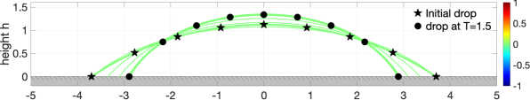
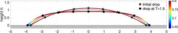
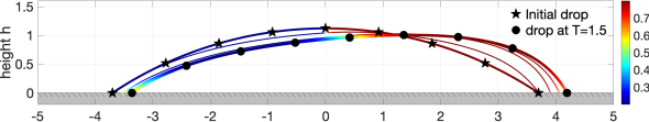
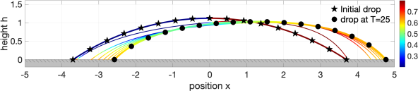
Figure 2. Spreading of droplets on a plane with lower surface tension due to the surfactant effect. 1st: Time evolution of the capillary surface without the surfactant starting from an initial profile (5.1) marked with black pentagrams to a doplet profile marked with black circles at the final time $T=1.5$. 2nd: With initial concentration $c=0.8$, the flatten droplet with a pancake shape is shown with a density-patched surface at $T=1.5$. 3rd: With an asymmetric initial concentration (5.4), an asymmetric evolution with the surfactant ’drag’ effect is shown at equal time intervals and at $T=1.5$. 4th: The asymmetric profile dragged by surfactant with initial concentration (5.4) turns out to be symmetric with approximated constant-concentration of surfactant at $T=25$.

5.2. Droplet on an inclined surface

In the second example, we compute the spreading of a droplet placed on an inclined substrate to observe the competition between the gravitational effect and the surfactant-dependent capillary effect due to the presence of different concentration of the surfactant.

We use the same initial droplet profile (5.1) and take the inclined angle $\theta_{0}=0.3$ for the substrate. We use the following computational parameters in Fig. 3

(5.5) $$\beta=0.1,\quad\kappa=0.5,\quad\gamma_{\scriptscriptstyle{\text{SL}}}-\gamma_{\scriptscriptstyle{\text{SG}}}=-0.75,\quad\xi=1,\quad D=0.1,\quad\Delta t=0.02,\quad N=800.$$

Same as Fig. 2, the evolution of the capillary surface is drawn at equal time intervals with solid thin lines and patched with color showing surfactant concentration.

In Fig. 3 (upper one), we take $c=0$ and compute the evolution of a droplet without surfactant as a comparison. We can observe the contact angle hysteresis (CAH) in the droplet profile at $T=2$ (marked with black circles) with an advancing contact angle and a receding contact angle due to the gravity, which is unapparent.

However, in Fig. 3 (middle one), to see the enhanced CAH due to the surfactant effect, we take an asymmetric initial concentration

(5.6) $$c(x,0)=0.45-\frac{0.5}{\pi}\arctan(100x),$$

which decreases from $0.7$ to $0.2$ with a sharp transition; see the patched curve marked with black pentagrams in Fig. 3 (middle one). As time increases, we see the gravity and the asymmetric concentration of the surfactant (left part higher than the right part of the capillary surface) accelerate the rolling down of the droplet. Then droplet profile at $T=2$ is marked with black circles and patched with the surfactant concentration, in which we observe a significant enhancement of CAH phenomena with very different advancing contact angles and receding contact angles. On the other hand, if we switch the initial concentration of the surfactant to

(5.7) $$c(x,0)=0.45+\frac{0.5}{\pi}\arctan(100x)$$

so that the right part has higher concentration than the left part of the capillary surface. Then in Fig. 3 (lower one), we observe the surfactant effect wins the competition with the gravity and the droplet even rises up instead of rolling down; see the droplet profile at $T=2$ (marked with black circles).

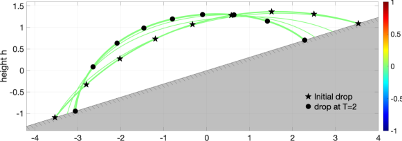
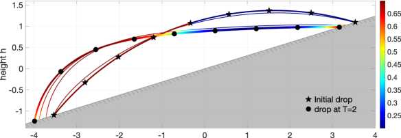
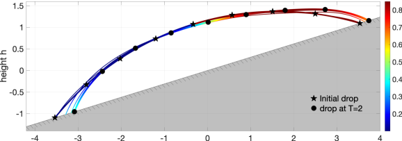
Figure 3. Enhanced CAH and resistance with the gravity due to asymmetric concentration of surfactant for a droplet placed on an inclined substrate with $\theta_{0}=0.3$. (upper) Time evolution of the capillary surface without the surfactant starting from an initial profile (5.1) marked with black pentagrams to a droplet profile marked with black circles at a final time $T=2$. (middle) With the initial concentration (5.6), the significant enhancement of rolling down and the CAH phenomena are shown with density-patched surfaces at equal time intervals and at $T=2$. (lower) With the initial concentration (5.7), the droplet rises up instead of rolling down because the surfactant effect wins the competition with the gravity.

5.3. Droplets on a textured substrate and in a cocktail glass

In the third example, we compute the spreading of a droplet on some typical textured substrates such as a cocktail glass and a substrate with constantly changed effective slope. The common computational parameters are

(5.8) $$\beta=0.1,\quad\kappa=0.5,\quad\xi=1;\quad D=0.5;\quad\Delta t=0.02.$$

In Fig. 4 (upper), we take the initial droplet profile (marked with black pentagrams) as

(5.9) $$h(x,0)=\sqrt{R^{2}-x^{2}}-R\cos(\theta_{\text{in}})+w(b_{0})+\frac{[w(b_{0})-w(-b_{0})](x+b_{0})}{2b_{0}},\quad\,\,R=\frac{b_{0}}{\theta_{\text{in}}},\quad b_{0}=3.7$$

with $\theta_{\text{in}}=\frac{3\pi}{16}$ and a cocktail glass substrate

(5.10) $$w(x)=0.5\sqrt{x^{2}+0.1}.$$

Then taking $\gamma_{\scriptscriptstyle{\text{SL}}}-\gamma_{\scriptscriptstyle{\text{SG}}}=-0.9,\,N=1600$ and the initial concentration of the surfactant as $c(x,0)=0.2$, time evolution of the density-patched capillary surfaces is shown at equal time intervals and at the final time $T=4$ (marked with black circles). We observe the capillary rise near the contact lines and the surfactant tends to push themselves and concentrate near the contact lines.

In Fig. 4 (lower), we take the initial droplet profile (marked with black pentagrams) as (5.9) with $\theta_{\text{in}}=\frac{1.3\pi}{8}$, an effective inclined angle $\theta_{0}=0.2$ and a textured substrate

(5.11) $$w(x)=0.1\left(\sin(2x)+\cos(4x)\right)^{2}.$$

Then taking $\gamma_{\scriptscriptstyle{\text{SL}}}-\gamma_{\scriptscriptstyle{\text{SG}}}=-0.5,\,N=800$ and the initial asymmetric concentration of the surfactant as

(5.12) $$c(x,0)=0.45+\frac{0.7}{\pi}\arctan(100x),$$

time evolution of the density-patched capillary surfaces is shown at equal time intervals and at final time $T=2$ (marked with black circles). We observe an asymmetric rising up of the droplet due to the asymmetric initial concentration and the constantly changed effective slope of the textured substrate.

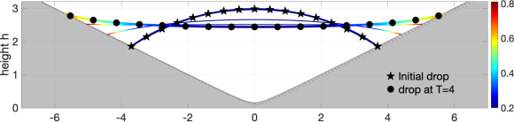
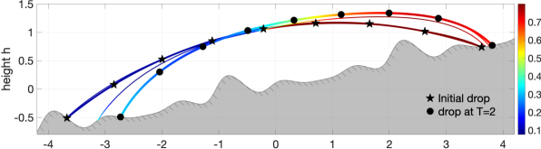
Figure 4. The upper figure is the time evolution of a droplet in a cocktail glass with a uniform initial concentration of surfactant. The initial profile (5.9) is marked with black pentagrams while the density-patched capillary surface at the final time $T=4$ is marked with black circles. The lower figure is the time evolution of a droplet on a inclined textured substrate (5.11). An asymmetric rising up starting from (5.12) is shown with the density-patched capillary surfaces at equal time intervals and at $T=2$.

Appendix A Proof of Proposition 2.1

Proof of Proposition 2.1.

Recall the continuity equation (2.20) on wetting domain $\Omega_{t}$ and the relation (2.14) between $c$ and $\mathcal{C}$. We then have

(A.1) $$0= \partial_{t}\left(c\sqrt{1+|\nabla h|^{2}}\right)+\nabla\cdot\left(c\sqrt{1+|\nabla h|^{2}}v_{xy}\right)$$

$$= \sqrt{1+|\nabla h|^{2}}\left((\partial_{t}+v_{xy}\cdot\nabla_{xy})c\right)+c\left(\partial_{t}\sqrt{1+|\nabla h|^{2}}+\nabla_{xy}\cdot\left(\sqrt{1+|\nabla h|^{2}}v_{xy}\right)\right)$$

$$= \sqrt{1+|\nabla h|^{2}}\left((\partial_{t}+v\cdot\nabla)\mathcal{C}\right)+\mathcal{C}\left(\partial_{t}\sqrt{1+|\nabla h|^{2}}+\nabla_{xy}\cdot\left(\sqrt{1+|\nabla h|^{2}}v_{xy}\right)\right)$$

where $v_{xy}:=\left(\begin{array}[]{c}v_{1}\\ v_{2}\end{array}\right)=\left(\begin{array}[]{c}\frac{-h_{t}h_{x}}{1+|\nabla h|^{2}}\\ \frac{-h_{t}h_{y}}{1+|\nabla h|^{2}}\end{array}\right)+\left(\begin{array}[]{c}f\\ g\end{array}\right)$ due to (2.17).

First, for the last term in (A.1), using the identity (2.35), we have

(A.2) $$\partial_{t}\sqrt{1+|\nabla h|^{2}}+\nabla_{xy}\cdot\left(\sqrt{1+|\nabla h|^{2}}v_{xy}\right)=h_{t}H+\nabla_{xy}\cdot\left(\sqrt{1+|\nabla h|^{2}}\left(\begin{array}[]{c}f\\ g\end{array}\right)\right)$$

This, together with (A.1), gives the equation for $\mathcal{C}$

(A.3) $$\left((\partial_{t}+v\cdot\nabla)\mathcal{C}\right)+\mathcal{C}v_{n}H+\frac{1}{\sqrt{1+|\nabla h|^{2}}}\nabla_{xy}\cdot\left(\sqrt{1+|\nabla h|^{2}}\left(\begin{array}[]{c}f\\ g\end{array}\right)\right)=0.$$

Second, we prove the following claim

(A.4) $$\nabla_{s}\cdot v_{s}=\frac{1}{\sqrt{1+|\nabla h|^{2}}}\nabla_{xy}\cdot\left(\sqrt{1+|\nabla h|^{2}}\left(\begin{array}[]{c}f\\ g\end{array}\right)\right)=\partial_{x}f+\partial_{y}g+\frac{1}{2}\left(\begin{array}[]{c}f\\ g\end{array}\right)\cdot\frac{\nabla_{xy}(|\nabla h|^{2})}{1+|\nabla h|^{2}}.$$

Denote

$$\tilde{f}(x,y,h(x,y,t))=f(x,y,t),\quad\tilde{g}(x,y,h(x,y,t)).$$

Then for the tangential velocity

(A.5) $$v_{s}=f\tau_{1}+g\tau_{2}=\left(\begin{array}[]{c}\tilde{f}\\ \tilde{g}\\ h_{x}\tilde{f}+h_{y}\tilde{g}\end{array}\right),$$

by the chain rule, we have

(A.6) $$\nabla\cdot v_{s}=\partial_{x}f+\partial_{y}g.$$

On the other hand,

(A.7) $$-n(n\cdot\nabla)v_{s}= -\frac{1}{1+|\nabla h|^{2}}\left(\begin{array}[]{c}-h_{x}\\ -h_{y}\\ 1\end{array}\right)\cdot(-h_{x}\partial_{x}-h_{y}\partial_{y}+\partial_{z})\left(\begin{array}[]{c}\tilde{f}\\ \tilde{g}\\ h_{x}\tilde{f}+h_{y}\tilde{g}\end{array}\right)$$

$$= \frac{1}{1+|\nabla h|^{2}}\left(f(h_{xx}+h_{xy})+g(h_{xy}+h_{yy})\right)=\frac{1}{2}\left(\begin{array}[]{c}f\\ g\end{array}\right)\cdot\frac{\nabla_{xy}(|\nabla h|^{2})}{1+|\nabla h|^{2}}.$$

Combining (A.6) and (A.7) yields (A.4). ∎

Appendix B Pseudo-code for first order scheme

Below, we present a pseudo-code for the first order scheme in Section 4.4.
1. Grid for time: $t^{n}=n\Delta t$, $n=0,1,\cdots,$ where $\Delta t$ is time step.
2. Fix $N$ and set moving grids for space: $x_{j}^{n}=a^{n}+{j}{\tau^{n}},\,\,\tau^{n}=\frac{b^{n}-a^{n}}{N}$, $j=-1,0,1,\cdots,N+1.$
3. Calculate volume $V:=\sum_{j=1}^{N-1}(h^{0}-w)(x^{0}_{j})\tau^{0}$.
4. Denote the finite difference operators

(B.1) $$(\partial_{x}h)_{0}^{n}=\frac{4h_{1}^{n}-h_{2}^{n}-3h_{0}^{n}}{2\tau^{n}},\quad(\partial_{x}h)_{N}^{n}=\frac{-4h_{N-1}^{n}+h_{N-2}^{n}+3h_{N}^{n}}{2\tau^{n}},$$

$$(\partial_{x}h)_{j}^{n}=\frac{h_{j+1}^{n}-h^{n}_{j-1}}{2\tau^{n}},\quad(\partial_{xx}h)_{j}^{n}=\frac{h^{n}_{j+1}-2h^{n}_{j}+h_{j-1}^{n}}{(\tau^{n})^{2}},\,\,j=1,\cdots,N-1.$$

Denote

$$(\partial_{x}w)_{0}:=\partial_{x}w(x^{n}_{0}),\quad(\partial_{x}w)_{N}:=\partial_{x}w(x^{n}_{N}),\quad\gamma_{i}^{n}:=\gamma(c_{i}^{n}),\quad i=0,\cdots,N.$$

5. Update $a^{n+1},b^{n+1}$, $j=0,1,\cdots,N$,

$$\xi\frac{a^{n+1}-a^{n}}{\Delta t} =\gamma_{0}^{n}\frac{1+(\partial_{x}h^{n})_{0}(\partial_{x}w)_{0}}{\sqrt{1+(\partial_{x}h^{n})_{0}^{2}}}+(\gamma_{\scriptscriptstyle{\text{SL}}}-\gamma_{\scriptscriptstyle{\text{SG}}})\sqrt{1+(\partial_{x}w)_{0}^{2}},$$

$$\xi\frac{b^{n+1}-b^{n}}{\Delta t} =-\gamma_{N}^{n}\frac{1+(\partial_{x}h^{n})_{N}(\partial_{x}w)_{N}}{\sqrt{1+(\partial_{x}h^{n})_{N}^{2}}}-(\gamma_{\scriptscriptstyle{\text{SL}}}-\gamma_{\scriptscriptstyle{\text{SG}}})\sqrt{1+(\partial_{x}w)_{N}^{2}}.$$

6. Update the moving grids $\,x_{j}^{n+1}=a^{n+1}+{j}{\tau^{n+1}},\,\,\tau^{n+1}=\frac{b^{n+1}-a^{n+1}}{N},\quad j=0,1,\cdots,N.$
7. From (4.22), $\,h_{j}^{n*}=h_{j}^{n}+(\partial_{x}h^{n})_{j}(a^{n+1}-a^{n}+j(\tau^{n+1}-\tau^{n})),\quad j=0,\cdots,N.$
8. Solve $h^{n+1}$ semi-implicitly
For $j=1,\cdots,N-1$, denote $\alpha_{j}=1+(h_{x}^{2})_{j}^{n}$ and solve

(B.2) $$\beta\alpha_{j}\frac{h_{j}^{n+1}-h^{n*}_{j}}{\Delta t}=\gamma_{j}^{n}\frac{h^{n+1}_{j+1}-2h^{n+1}_{j}+h^{n+1}_{j-1}}{(\tau^{n+1})^{2}}-\kappa\alpha_{j}^{3/2}(h_{j}^{n+1}\cos\theta_{0}+x^{n+1}_{j}\sin\theta_{0})+\lambda^{n+1}\alpha_{j}^{3/2},$$

$$\sum_{j=1}^{N-1}(h^{n+1}_{j}-w(x_{j}^{n+1}))\tau^{n+1}=V,$$

with the Dirichlet boundary condition $h^{n+1}_{0}=w(x^{n+1}_{0}),\,\,h^{n+1}_{N}=w(x_{N}^{n+1})$.

Denote a positive-definite matrix $A_{(N-1)\times(N-1)}=(a_{ij})$ with

(B.3) $$\begin{array}[]{c}a_{j,j-1}:=-\gamma_{j}^{n},\,\,a_{j,j+1}:=-\gamma_{j}^{n},\quad a_{j,j}:=2\gamma_{j}^{n}+\frac{\beta(\tau^{n+1})^{2}}{\Delta t}\alpha_{j}+\kappa\cos\theta_{0}(\tau^{n+1})^{2}\alpha_{j}^{\frac{3}{2}}\end{array}$$

and a vector of length $N-1$

$$\tilde{f}_{j}:=\frac{\beta(\tau^{n+1})^{2}}{\Delta t}h_{j}^{n*}\alpha_{j}-\kappa\sin\theta_{0}x_{j}^{n+1}(\tau^{n+1})^{2}\alpha_{j}^{\frac{3}{2}},\quad j=1,\cdots,N-1$$

and (B.2) becomes for $j=1,\cdots,N-1$,

(B.4) $$a_{j,j-1}h^{n+1}_{j-1}+a_{j,j}h^{n+1}_{j}+a_{j,j+1}h^{n+1}_{j+1}-\alpha_{j}^{\frac{3}{2}}(\tau^{n+1})^{2}\lambda^{n+1}=\tilde{f}_{j}.$$

Denote

(B.5) $$f_{1}=\tilde{f}_{1}+\gamma_{1}^{n}w(x_{0}^{n+1}),\,\,\{f_{j}=\tilde{f}_{j}\}_{j=2}^{N-2},\,\,f_{N-1}=\tilde{f}_{N-1}+\gamma_{N-1}^{n}w(x_{N}^{n+1}),\,\,f_{N}:=\sum_{j=1}^{N-1}w(x_{j}^{n+1})+\frac{V}{\tau^{n+1}}.$$

The resulting linear system $\bar{A}y=f$ has a non-singular matrix $\bar{A}=\left(\begin{array}[]{cc}A&\alpha^{\frac{3}{2}}\\ e^{\top}&0\end{array}\right)_{N\times N},$ where $y^{\top}=(h^{n+1}_{1},\cdots,h^{n+1}_{N-1},-(\tau^{n+1})^{2}\lambda^{n+1})$ and $e^{\top}=(1,\cdots,1)\in\mathbb{R}^{N-1}$.
9. Solve $c^{n+1}$ from (4.25) implicitly.

Denote

$$(h_{t})_{j}^{n+1}:=\frac{h_{j}^{n+1}-h_{j}^{n*}}{\Delta t},\quad j=1,\cdots,N-1,$$

$$\tilde{f}_{j}:=-D\frac{(h_{x})_{j}^{n+1}(h_{xx})_{j}^{n+1}}{1+(h_{x}^{2})_{j}^{n+1}}(c_{x})_{j}^{n}+(h_{t})_{j}^{n+1}(h_{x})_{j}^{n+1}(c_{x})_{j}^{n}+\frac{(h_{t})_{j}^{n+1}(h_{xx})_{j}^{n+1}}{1+(h_{x}^{2})_{j}^{n+1}}c_{j}^{n}.$$

Then (4.25) becomes

(B.6) ,

$$(1+(h_{x}^{2})_{j}^{n+1})\frac{c^{n+1}_{j}-c^{n}_{j}}{\Delta t}=D\frac{c^{n+1}_{j+1}-2c^{n+1}_{j}+c^{n+1}_{j-1}}{(\tau^{n+1})^{2}}+\tilde{f}_{j},\quad j=1,\cdots,N-1$$

with boundary conditions

(B.7) $$D(c_{x})^{n+1}_{0}+c^{n+1}_{0}(1+(h_{x})_{0}(w_{x})_{0})\frac{a^{n+1}-a^{n}}{\Delta t}=0,$$

$$D(c_{x})^{n+1}_{N}+c^{n+1}_{N}(1+(h_{x})_{N}(w_{x})_{N})\frac{b^{n+1}-b^{n}}{\Delta t}=0,$$

where

$$(\partial_{x}c)_{0}^{n+1}=\frac{4c_{1}^{n+1}-c_{2}^{n+1}-3c_{0}^{n+1}}{2\tau^{n+1}},\quad(\partial_{x}c)_{N}^{n+1}=\frac{-4c_{N-1}^{n+1}+c_{N-2}^{n+1}+3c_{N}^{n+1}}{2\tau^{n+1}}.$$

Let

$$\iota_{0}:=\frac{2\tau^{n+1}}{D}(1+(h_{x})_{0}(w_{x})_{0})\frac{a^{n+1}-a^{n}}{\Delta t},\quad\iota_{N}:=\frac{2\tau^{n+1}}{D}(1+(h_{x})_{N}(w_{x})_{N})\frac{b^{n+1}-b^{n}}{\Delta t},$$

then boundary condition (B.7) becomes

$$(\iota_{0}-3)c_{0}^{n+1}+4c_{1}^{n+1}-c_{2}^{n+1}=0,\quad c_{N-2}^{n+1}-4c_{N-1}^{n+1}+(\iota_{N}+3)c_{N}^{n+1}=0.$$

Now we recast (B.6) in a $N+1$ order matrix form

$$Bc^{n+1}=f,\quad B=(b_{ij})_{i,j=0,\cdots,N}$$

where, for $i=0$, $b_{00}=\iota_{0}-3,\quad b_{01}=4,\quad b_{02}=-1;$ for $i=1,\cdots,N-1$, $b_{i,i-1}=-1,\quad b_{i,i}=2+\frac{(\tau^{n+1})^{2}}{D\Delta t}(1+(h_{x}^{2})_{i}^{n+1}),\quad b_{i,i+1}=-1;$ for $i=N$, $b_{N,N-2}=1,b_{N,N-1}=-4,b_{N,N}=\iota_{N}+3,$ and $f_{0}=0,f_{N}=0,f_{i}=\frac{(\tau^{n+1})^{2}}{D}\left(\tilde{f}_{i}+\frac{1+(h_{x}^{2})_{i}^{n+1}}{\Delta t}c^{n}_{j}\right),\,\,i=1,\cdots,N-1.$

References

- [1] P. Cermelli, E. Fried, and M. Gurtin. Transport relations for surface integrals arising in the formulation of balance laws for evolving fluid interfaces. Journal of Fluid Mechanics, 544:339–351, 2005.
- [2] K.-Y. Chen and M.-C. Lai. A conservative scheme for solving coupled surface-bulk convection–diffusion equations with an application to interfacial flows with soluble surfactant. Journal of Computational Physics, 257:1–18, 2014.
- [3] W.-L. Chou, P.-Y. Lee, C.-L. Yang, W.-Y. Huang, and Y.-S. Lin. Recent advances in applications of droplet microfluidics. Micromachines, 6(9):1249–1271, 2015.
- [4] R. V. Craster and O. K. Matar. Dynamics and stability of thin liquid films. Reviews of Modern Physics, 81(3):1131–1198, Aug 2009.
- [5] P. G. de Gennes. Wetting: statics and dynamics. Reviews of Modern Physics, 57(3):827–863, Jul 1985.
- [6] P.-G. De Gennes, F. Brochard-Wyart, and D. Quéré. Capillarity and wetting phenomena: drops, bubbles, pearls, waves. Springer Science & Business Media, 2013.
- [7] L. Desvillettes and C. Villani. On a variant of korn’s inequality arising in statistical mechanics. ESAIM: Control, Optimisation and Calculus of Variations, 8:603–619, 2002.
- [8] M. Doi. Soft matter physics. Oxford University Press, first edition edition, 2013.
- [9] M. Doi. Soft matter physics. Oxford University Press, 2013.
- [10] M. Doi. Onsager principle in polymer dynamics. Progress in Polymer Science, 112:101339, Jan 2021.
- [11] S. Ganesan. Simulations of impinging droplets with surfactant-dependent dynamic contact angle. Journal of Computational Physics, 301:178–200, Nov 2015.
- [12] Y. Gao, H. Ji, J.-G. Liu, and T. P. Witelski. Global existence of solutions to a tear film model with locally elevated evaporation rates. Physica D: Nonlinear Phenomena, 350:13–25, 2017.
- [13] Y. Gao and J.-G. Liu. Projection method for droplet dynamics on groove-textured surface with merging and splitting. arXiv preprint arXiv:2005.07851, 2020.
- [14] Y. Gao and J.-G. Liu. Gradient flow formulation and second order numerical method for motion by mean curvature and contact line dynamics on rough surface. Interfaces and Free boundaries, 23(1):130–158, 2021.
- [15] H. Garcke and S. Wieland. Surfactant spreading on thin viscous films: Nonnegative solutions of a coupled degenerate system. SIAM Journal on Mathematical Analysis, 37(6):2025–2048, Jan 2006.
- [16] H. Goldstein, C. Poole, and J. Safko. Classical mechanics. 3rd, 2002.
- [17] N. Grunewald and I. Kim. A variational approach to a quasi-static droplet model. Calculus of Variations and Partial Differential Equations, 41(1–2):1–19, May 2011.
- [18] Y. Guo and I. Tice. Stability of contact lines in fluids: 2d stokes flow. Archive for Rational Mechanics and Analysis, 227(2):767–854, Feb 2018.
- [19] M. E. Gurtin. Configurational forces as basic concepts of continuum physics, volume 137. Springer Science & Business Media, 1999.
- [20] G. Karapetsas, R. V. Craster, and O. K. Matar. On surfactant-enhanced spreading and superspreading of liquid drops on solid surfaces. Journal of Fluid Mechanics, 670:5–37, Mar 2011.
- [21] G. Karapetsas, K. C. Sahu, and O. K. Matar. Evaporation of sessile droplets laden with particles and insoluble surfactants. Langmuir, 32(27):6871–6881, Jul 2016.
- [22] M.-C. Lai. Numerical simulation of moving contact lines with surfactant by immersed boundary method. Communications in Computational Physics, 8(4):735–757, Jun 2010.
- [23] M.-C. Lai, Y.-H. Tseng, and H. Huang. An immersed boundary method for interfacial flows with insoluble surfactant. Journal of Computational Physics, 227(15):7279–7293, 2008.
- [24] L. Limat and H. Stone. Three-dimensional lubrication model of a contact line corner singularity. EPL (Europhysics Letters), 65(3):365, 2004.
- [25] A. Marchand, J. H. Weijs, J. H. Snoeijer, and B. Andreotti. Why is surface tension a force parallel to the interface? American Journal of Physics, 79(10):999–1008, 2011.
- [26] A. A. Olajire. Review of asp eor (alkaline surfactant polymer enhanced oil recovery) technology in the petroleum industry: Prospects and challenges. Energy, 77:963–982, 2014.
- [27] T. Qian, X.-P. Wang, and P. Sheng. A variational approach to moving contact line hydrodynamics. Journal of Fluid Mechanics, 564:333, Oct 2006.
- [28] N. Shembekar, C. Chaipan, R. Utharala, and C. A. Merten. Droplet-based microfluidics in drug discovery, transcriptomics and high-throughput molecular genetics. Lab on a Chip, 16(8):1314–1331, 2016.
- [29] H. A. Stone. A simple derivation of the time‐dependent convective‐diffusion equation for surfactant transport along a deforming interface. Physics of Fluids A: Fluid Dynamics, 2(1):111–112, Jan 1990.
- [30] I. Tice and L. Wu. Dynamics and stability of sessile drops with contact points. Journal of Differential Equations, 272:648 – 731, 2021.
- [31] M. Wu, Y. Di, X. Man, and M. Doi. Drying droplets with soluble surfactants. Langmuir, 35(45):14734–14741, 2019.
- [32] J.-J. Xu and W. Ren. A level-set method for two-phase flows with moving contact line and insoluble surfactant. Journal of Computational Physics, 263:71–90, 2014.
- [33] X. Xu, Y. Di, and M. Doi. Variational method for contact line problems in sliding liquids. Phys. Fluids, 28:087101, 2016.
- [34] Z. Zhang, S. Xu, and W. Ren. Derivation of a continuum model and the energy law for moving contact lines with insoluble surfactants. Physics of Fluids, 26(6):062103, Jun 2014.