Dissipative dynamics of a particle coupled to field via internal degrees of freedom

Abstract

We study the non-equilibrium dissipative dynamics of the center of mass of a particle coupled to a field via its internal degrees of freedom. We model the internal and external degrees of freedom of the particle as quantum harmonic oscillators in 1+1 D, with the internal oscillator coupled to a scalar quantum field at the center of mass position. Such a coupling results in a nonlinear interaction between the three pertinent degrees of freedom – the center of mass, internal degree of freedom, and the field. It is typically assumed that the internal dynamics is decoupled from that of the center of mass owing to their disparate characteristic time scales. Here we use an influence functional approach that allows one to account for the self-consistent backaction of the different degrees of freedom on each other, including the coupled non-equilibrium dynamics of the internal degree of freedom and the field, and their influence on the dissipation and noise of the center of mass. Considering a weak nonlinear interaction term, we employ a perturbative generating functional approach to derive a second order effective action and a corresponding quantum Langevin equation describing the non-equilibrium dynamics of the center of mass. We analyze the resulting dissipation and noise arising from the field and the internal degree of freedom as a composite environment. Furthermore, we establish a generalized fluctuation-dissipation relation for the late-time dissipation and noise kernels. Our results are pertinent to open quantum systems that possess intermediary degrees of freedom between system and environment, such as in the case of optomechanical interactions.

I Introduction

Dissipative non-equilibrium dynamics of complex quantum systems comprising different degrees of freedom is a subject of significant interest from the perspective of theory of open quantum systems, as well as, emerging quantum information applications and devices BPBook ; Weiss ; Clerk20 . While the dissipative dynamics of a reduced quantum system coupled linearly to its environment has been studied extensively, the case of a nonlinear coupling between a system and its environment via an intermediate degree of freedom and its effect on the resulting dynamics is seldom discussed HPZ93 ; Maghrebi16 ; Lampo16 . A commonly employed assumption is that the time-scales associated with the different degrees of freedom are sufficiently disparate so that their dynamics can be treated as being effectively decoupled from each other Stenholm86 ; Lan08 ; Haake . Such an assumption precludes the possibility of studying the rich interplay between the different degrees of freedom, and its effect on the non-equilibrium dynamics of the system of interest. Moreover, an adiabatic elimination of fast variables does not allow one to see the effects of the non-equilibrium dynamics and quantum fluctuations of the fast degrees of freedom on the system dissipation and noise.

A canonical example of such a complex open quantum system is the optomechanical interaction between a neutral polarizable particle and a field, for instance, a moving atom, nanoparticle, or molecule interacting with the electromagnetic (EM) field Wieman ; Yin ; Molecules . As an essential feature these systems possess internal electronic degrees of freedom that interact with the EM field and are located at the center of mass position represented by the mechanical degree of freedom (MDF). While the MDF of the particle does not couple to the EM field directly, its internal degrees of freedom (IDF) interact with the EM field at the center of mass position, thus mediating an effective coupling between the MDF and the field. Considering the MDF as the system of interest, with the EM field and the IDF acting as an environment, such an effective interaction leads to dissipation and noise in system dynamics. There is an interesting interplay between the three degrees of freedom (the MDF, the IDF, and the EM field) that takes place in such a scenario as has been previously explored in KSthesis ; MOF1 ; MOF2 ; Wang14 . Considering the dynamics from an approach that includes the self-consistent backaction of all the degrees of freedom on each other allows one to examine the role of IDF in the center of mass dynamics. For example, it has been shown that the IDF can facilitate a transfer of correlations between the field and center of mass in the case of optomechanical interactions KSthesis ; MOF2 and affect the center of mass decoherence Brun16 . On the other hand, it has also been demonstrated that including the quantized center of mass motion can affect the radiation reaction and thermalization of the IDF AERL19 .

We study here a minimal model that captures the interplay between different degrees of freedom in a composite system and the nonequilibrium dissipative center of mass dynamics. Such a model forms the basis for optomechanical interactions between neutral particles and fields, and more generally applies to open quantum systems that couple to an environment via internal degrees of freedom. The remainder of this paper is organized as follows. In Section II we describe the model in consideration, in Section III we describe the derivation of a second order effective action for the center of mass by integrating out the IDF and the field using a perturbative influence functional approach HPZ93 . In Section IV we write an effective Langevin equation for the center of mass, discuss the resulting dynamics and present a generalized fluctuation-dissipation relation. We summarize our findings and present an outlook of the work in Section V.

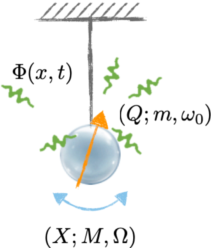
Figure 1: Schematic representation of a mechanical oscillator of mass $M$ and frequency $\Omega$ coupled to a massless scalar field $\Phi$ via an IDF. The internal oscillator with position coordinate $Q$ is described as a harmonic oscillator of mass $m$ and frequency $\omega_{0}$ and couples to the scalar field $\Phi\left({x},t\right)$ at the center of mass position ${X}$ of the mechanical oscillator.

II Model

Let us consider a particle with its center of mass described by a mechanical oscillator of mass $M$ and frequency $\Omega$, and its polarization described by an IDF as a harmonic oscillator of mass $m$ and resonance frequency $\omega_{0}$. The composite system is assumed to be interacting with a quantum field, which we consider to be a scalar field $\Phi(x,t)$ in $1+1$ D. The total action of the system can be written as

$$S=S_{M}+S_{I}+S_{F}+S_{\mathrm{int},}$$ (1)

where

$$S_{M} =\int\mathrm{d}\tau\left(\frac{1}{2}M\dot{X}^{2}-\frac{1}{2}M\Omega^{2}X^{2}\right)$$ (2)

refers to the free action for the mechanical oscillator with $\left\{X,\dot{X}\right\}$ referring to the center of mass position and velocity, while

$$S_{I} =\int\mathrm{d}\tau\left(\frac{1}{2}m\dot{Q}^{2}-\frac{1}{2}m\omega_{0}^{2}Q^{2}\right)$$ (3)

corresponds to the free action for the internal degree of freedom with amplitude $Q$, and

$$S_{F} =\int\mathrm{d}\tau\int\mathrm{d}{x}\frac{\epsilon_{0}}{2}\left[\left(\partial_{t}\Phi(x,\tau)\right)^{2}-\left({\mathbf{\partial}_{x}}\Phi(x,\tau)\right)^{2}\right]$$ (4)

is the free action for the scalar field $\Phi\left(x,t\right)$, $\epsilon_{0}$ being the vacuum permittivity. We consider $\hbar=c=1$ throughout this paper. The correspondence with the EM field is established by identifying the scalar field $\Phi\left({x},t\right)$ as the vector potential.

Considering that the particle interacts with the field via its IDF, at the position determined by the MDF, the interaction action is given as

$$S_{\mathrm{int}} =\int\mathrm{d}\tau\int\mathrm{d}{x}\lambda Q\Phi({x},\tau)\delta\left({x}-X(\tau)\right)$$ (5)

with the strength of the interaction defined by $\lambda$. We note that the above interaction action is nonlinear, with the two degrees of freedom and the field interacting together. Such a model, previously referred to as the mirror-oscillator-field model has been studied in the context of describing optomechanical interactions from a microscopic perspective MOF1 ; MOF2 ; KSthesis . It provides a self-consistent treatment of the different degrees of freedom involved, in that one does not need to impose the boundary conditions on the field by hand, and the mechanical effects of the field are consistently described upon tracing over the IDF.

In typical experimental systems of relevance, such as those of atoms and nanoparticles confined in traps, the center of mass motion is restricted to a region of the space smaller than the wavelengths of the field that interact resonantly with the internal degrees. Thus motivated by practical considerations, we assume that the motion of the MDF is restricted to small displacements about the average equilibrium position $X_{0}$, such that we can expand the interaction action to first order in displacements from the equilibrium as follows

$$S_{\mathrm{int}} \approx\int\mathrm{d}\tau\left[\lambda Q\Phi(X_{0},\tau)+\lambda Q\partial_{x}\Phi(X_{0},\tau)\left(X-X_{0}\right)\right].$$ (6)

The first term in the above action represents the linear interaction between the IDF and the field, similar to the $\sim{\mathbf{p}}\cdot{\mathbf{A}}$ coupling in atom-field interactions. The second term stands for the tripartite interaction between the IDF, the MDF and the field. Thus, as we show in the following, the effective coupling of the center of mass to the field via the IDF leads to its dissipative dynamics. From now on, for simplicity and without loss of generality, we assume $X_{0}=0$.

II.1 Scalar field as bath of harmonic oscillators

The above separation of the total interaction action (Eq.(6)) suggests splitting the field into two separate oscillator baths such that one of the baths interacts with the IDF, while the other is coupled to both the internal and mechanical degrees. We thus make an eigenmode decomposition of the field to rewrite it in terms of a bath of oscillators as follows QBM3

$$\Phi({x},\tau)=\sum_{n}\sqrt{\frac{1}{\epsilon_{0}{L}}}\left[q_{n}^{(-)}\cos({\omega}_{n}{x})+q_{n}^{(+)}\sin({\omega}_{n}{x})\right],$$ (7)

where $L$ is the mode volume of the field, $\omega_{n}$ refers to the mode frequency, and $q_{n}^{(+)}$ and $q_{n}^{(-)}$ refer to two independent set of eigenmodes of the field, assuming periodic boundary conditions. One can thus rewrite the free field action as as a sum $S_{F}=S_{F}^{(+)}+S_{F}^{(-)}$, where

$$S_{F}^{(\pm)}=\int\mathrm{d}\tau\sum_{n}\frac{1}{2}\left[\left.\dot{q}_{n}^{(\pm)}\right.^{2}-\omega_{n}^{2}\left.{q}_{n}^{(\pm)}\right.^{2}\right]$$ (8)

with $S_{F}^{(\pm)}$ corresponding to two separate baths of $(+)$ and $(-)$ oscillators. Thus, for $X_{0}=0$ the interaction action in Eq.(6) can be written as a sum of two separate interaction terms $S_{\mathrm{int}}=S_{\mathrm{int}}^{(-)}+S_{\mathrm{int}}^{(+)}$, with

$$S_{\mathrm{int}}^{(-)} =\int\mathrm{d}\tau\lambda Q\sum_{n}q_{n}^{(-)}$$ (9)

$$S_{\mathrm{int}}^{(+)} =\int\mathrm{d}\tau\lambda Q\sum_{n}\omega_{n}Xq_{n}^{(+)}.$$ (10)

Thus the interaction action $S_{\mathrm{int}}^{(-)}$ linearly couples the $(-)$ bath of oscillators of the scalar field to the IDF, leading to the dissipative dynamics of the IDF. The interaction action $S_{\mathrm{int}}^{(+)}$ couples the center of mass to the $(+)$ bath of oscillators via the IDF. We note that $S_{\mathrm{int}}^{(+)}$ is essentially responsible for all the mechanical effects of the field, such as radiation pressure due to optical fields and vacuum-induced forces PierreBook ; PeterQOBook . For instance, one can see that eliminating the IDF from the interaction action $S_{\mathrm{int}}^{(+)}$ yields an effective nonlinear interaction between the MDF and the field, similar to the intensity-position coupling in optomechanical interactions KSthesis . We also remark here that the above separation of the field into two uncorrelated baths is akin to the Einstein-Hopf theorem that establishes the statistical independence of the blackbody radiation field and its derivative EinHopf1 ; EinHopf3 .

III Effective action derivation from perturbative influence functional approach

The nonlinearity of the interaction action $S_{\mathrm{int}}^{(+)}$ limits the possibility of obtaining an exact analytical solution for the center of mass dynamics. We therefore follow a perturbative generating functional approach as prescribed in HPZ93 , assuming that the characteristic nonlinear coupling strength $\left(\sim\lambda\omega_{n}\right)$ can be treated perturbatively to write the resulting dynamics of the center of mass.

Let us consider the evolution of the system density matrix $\hat{\rho}_{M}$ as follows

$$\hat{\rho}_{M}\left(t\right)=\mathrm{Tr}_{I}\mathrm{Tr}_{F^{+}}\mathrm{Tr}_{F^{-}}\left[\hat{\mathcal{U}}(t,0)\left(\hat{\rho}_{M}(0)\otimes\hat{\rho}_{I}(0)\otimes\hat{\rho}_{F}^{(+)}(0)\otimes\hat{\rho}_{F}^{(-)}(0)\right)\hat{\mathcal{U}}^{\dagger}(t,0)\right],$$ (11)

where we have assumed that the density operators for the different degrees of freedom are initially uncorrelated with each other, with $\hat{\rho}_{I}$ and $\hat{\rho}_{F}^{(\pm)}$ referring to the density matrices for the IDF and the $(\pm)$ bath, and $\hat{\mathcal{U}}(t,0)$ corresponding to the time evolution operator. We write the density matrices in a coordinate representation such that

$$\hat{\rho}_{M}(\tau)= \int\mathrm{d}X\mathrm{d}X^{\prime}\rho_{M}\left(X,X^{\prime};\tau\right)\left|X\right\rangle\left\langle X^{\prime}\right|,$$ (12)

$$\hat{\rho}_{I}(\tau)= \int\mathrm{d}Q\mathrm{d}Q^{\prime}\rho_{I}\left(Q,Q^{\prime};\tau\right)\left|Q\right\rangle\left\langle Q^{\prime}\right|,$$ (13)

$$\hat{\rho}_{F}^{(\pm)}(\tau)= \prod_{n}\int\mathrm{d}q_{n}^{(\pm)}\mathrm{d}{q^{(\pm)}_{n}}^{\prime}\rho_{F}^{(\pm)}\left(\left\{q_{n}^{(\pm)},{q^{(\pm)}_{n}}^{\prime}\right\};\tau\right)\left|q_{n}^{(\pm)}\right\rangle\left\langle{q^{(\pm)}_{n}}^{\prime}\right|,$$ (14)

such that the system evolution in Eq. (11) can be rewritten as

$$\rho_{M}\left({X}_{f},{X}_{f}^{\prime};t\right)= \prod_{m,n}\int\mathrm{d}Q_{f}\mathrm{d}q^{(+)}_{nf}\mathrm{d}q^{(-)}_{mf}\int\mathrm{d}{X}_{i}\mathrm{d}Q_{i}\mathrm{d}q^{(+)}_{ni}\mathrm{d}q^{(-)}_{mi}\int\mathrm{d}{X}_{i}^{\prime}\mathrm{d}Q_{i}^{\prime}\mathrm{d}{q^{(+)}_{ni}}^{\prime}\mathrm{d}{q^{(-)}_{mi}}^{\prime}$$

$$\left[\rho_{M}\left({X}_{i},{X}_{i}^{\prime};0\right)\otimes\rho_{I}\left(Q_{i},Q_{i}^{\prime};0\right)\otimes\rho_{F}\left(\left\{q^{(+)}_{ni},{q^{(+)}_{ni}}^{\prime}\right\};0\right)\otimes\rho_{F}\left(\left\{q^{(-)}_{mi},{q^{(-)}_{mi}}^{\prime}\right\};0\right)\right.$$

$$\left.\mathcal{J}\left(X_{f},Q_{f},\left\{{q_{nf}^{(+)}},{q_{mf}^{(-)}}\right\};t\big{|}X_{i},Q_{i},\left\{{q_{ni}^{(+)}},{q_{mi}^{(-)}}\right\};0\right)\mathcal{J}^{\dagger}\left(X^{\prime}_{f},Q_{f},\left\{{q_{nf}^{(+)}},{q_{mf}^{(-)}}\right\};t\big{|}X^{\prime}_{i},Q^{\prime}_{i},\left\{{q_{ni}^{(+)}}^{\prime},{q_{mi}^{(-)}}^{\prime}\right\};0\right)\right],$$ (15)

where $\left\{{X}_{i},{X}_{i}^{\prime}\right\}$ and $\left\{{X}_{f},{X}_{f}^{\prime}\right\}$ refer to the initial and final coordinates corresponding to the center of mass variables respectively, $\left\{Q_{i},Q_{i}^{\prime};Q_{f},Q_{f}^{\prime}\right\}$ are those for the internal oscillator, and $\left\{q_{ni}^{(\pm)},{q_{ni}^{(\pm)}}^{\prime};q_{nf}^{(\pm)},{q_{nf}^{(\pm)}}^{\prime}\right\}$ are the initial and final coordinates for the $n^{\mathrm{th}}$ oscillator of the $(\pm)$ bath. We assume that the initial states $\rho_{F}^{(\pm)}\left(\left\{q^{(\pm)}_{ni},{q^{(\pm)}_{ni}}^{\prime}\right\};0\right)$ of the field and $\rho_{I}\left(Q_{i},Q_{i}^{\prime};0\right)$ of the IDF are thermal with a temperature $T_{F}$ and $T_{I}$ respectively. The forward propagator is defined as $\mathcal{J}\left(X_{f},Q_{f},\left\{q_{nf}^{(+)},q_{mf}^{(-)}\right\};t\big{|}X_{i},Q_{i},\left\{q_{ni}^{(+)},q_{mi}^{(-)}\right\};0\right)\equiv\prod_{m,n}\left\langle{X}_{f}\right|\left\langle Q_{f}\right|\left\langle q^{(+)}_{nf}\right|\left\langle q^{(-)}_{mf}\right|\hat{\mathcal{U}}\left(t,0\right)\left|q^{(-)}_{mi}\right\rangle\left|q^{(+)}_{ni}\right\rangle\left|Q_{i}\right\rangle\left|{X}_{i}\right\rangle$. Thus the first and last terms in the integral refer to the forward and backward propagators that can be expressed in path integral representation to write the evolution as

$$\rho_{M}\left({X}_{f},{X}_{f}^{\prime};t\right)=\int\mathrm{d}{X}_{i}\int\mathrm{d}{X}_{i}^{\prime}\,\rho_{M}\left({X}_{i},{X}_{i}^{\prime};0\right)\int_{{X}(0)={X}_{i}}^{{X}(t)={X}_{f}}\mathcal{D}{X}\int_{{X}^{\prime}(0)={X}^{\prime}_{i}}^{{X}^{\prime}(t)=X^{\prime}_{f}}\mathcal{D}{X}^{\prime}e^{i\left(S_{M}[{X}]-S_{M}[{X}^{\prime}]\right)}\mathcal{F}\left[{X},{X}^{\prime}\right],$$ (16)

where $\mathcal{F}\left[{X},{X}^{\prime}\right]$ refers to the influence functional of the field and the internal oscillator acting on the MDF FeynmanTrick , which can be written explicitly as

$$\mathcal{F}\left[{X},{X}^{\prime}\right]\equiv$$

$$\prod_{m,n}\int\mathrm{d}Q_{f}\mathrm{d}q^{(+)}_{nf}\mathrm{d}q^{(-)}_{mf}\int\mathrm{d}Q_{i}\mathrm{d}q^{(+)}_{ni}\mathrm{d}q^{(-)}_{mi}\int\mathrm{d}Q_{i}^{\prime}\mathrm{d}{q^{(+)}_{ni}}^{\prime}\mathrm{d}{q^{(-)}_{mi}}^{\prime}\rho_{I}\left(Q_{i},Q_{i}^{\prime};0\right)\otimes\rho_{F}^{(+)}\left(\left\{q^{(+)}_{ni},{q^{(+)}_{ni}}^{\prime}\right\};0\right)\otimes\rho_{F}^{(-)}\left(\left\{q^{(-)}_{mi},{q^{(-)}_{mi}}^{\prime}\right\};0\right)$$

$$\int_{Q(0)=Q_{i}}^{Q(t)=Q_{f}}\mathcal{D}Q\int_{Q^{\prime}(0)=Q^{\prime}_{i}}^{Q^{\prime}(t)=Q_{f}}\mathcal{D}Q^{\prime}e^{i\left(S_{I}[Q]-S_{I}[Q^{\prime}]\right)}\int_{q^{(+)}_{n}(0)=q^{(+)}_{ni}}^{q^{(+)}_{n}(t)=q^{(+)}_{nf}}\mathcal{D}q_{n}^{(+)}\int_{{q^{(+)}_{n}}^{\prime}(0)={q^{(+)}_{ni}}^{\prime}}^{{q^{(+)}_{n}}^{\prime}(t)=q^{(+)}_{nf}}\mathcal{D}{q^{(+)}_{n}}^{\prime}e^{i\left(S_{F}^{(+)}\left[\left\{q_{n}^{(+)}\right\}\right]-S_{F}^{(+)}\left[\left\{{q_{n}^{(+)}}^{\prime}\right\}\right]\right)}$$

$$\int_{q^{(-)}_{m}(0)=q^{(-)}_{mi}}^{q^{(-)}_{m}(t)=q^{(-)}_{mf}}\mathcal{D}q_{m}^{(-)}\int_{{q^{(-)}_{m}}^{\prime}(0)={q^{(-)}_{mi}}^{\prime}}^{{q^{(-)}_{m}}^{\prime}(t)=q^{(-)}_{mf}}\mathcal{D}{q^{(-)}_{m}}^{\prime}e^{i\left(S_{F}^{(-)}\left[\left\{q_{m}^{(-)}\right\}\right]-S_{F}^{(-)}\left[\left\{{q_{m}^{(-)}}^{\prime}\right\}\right]\right)}e^{i\left(S_{\mathrm{int}}^{(-)}\left[Q,\left\{q_{m}^{(-)}\right\}\right]-S_{\mathrm{int}}^{(-)}\left[Q^{\prime},\left\{{q_{m}^{(-)}}^{\prime}\right\}\right]\right)}$$

$$e^{i\left(S_{\mathrm{int}}^{(+)}\left[{X},Q,\left\{q_{n}^{(+)}\right\}\right]-S_{\mathrm{int}}^{(+)}\left[{X}^{\prime},Q^{\prime},\left\{{q_{n}^{(+)}}^{\prime}\right\}\right]\right)}.$$ (17)

Thus we have treated here the MDF as the system and the IDF and the field as the bath, with the influence functional capturing the influence of the bath on the evolution of the MDF. We will now evaluate the influence functional in a perturbative manner, by first tracing out the $(-)$ bath modes that couple only to the IDF, and then the $(+)$ bath modes and the IDF that couple to the center of mass.

III.1 Tracing over the $(-)$ bath

Let us define ${\mathcal{F}^{(-)}\left[Q,Q^{\prime}\right]}$ as the influence functional that accounts for the influence of the $(-)$ bath on the IDF as follows

$$\mathcal{F}^{(-)}\left[Q,Q^{\prime}\right]\equiv\prod_{m}\int\mathrm{d}q^{(-)}_{mf}\int\mathrm{d}q^{(-)}_{mi}\mathrm{d}{q^{(-)}_{mi}}^{\prime}\rho_{F}^{(-)}\left(\left\{q^{(-)}_{mi},{q^{(-)}_{mi}}^{\prime}\right\};0\right)\int_{q^{(-)}_{m}(0)=q^{(-)}_{mi}}^{q^{(-)}_{m}(t)=q^{(-)}_{mf}}\mathcal{D}q_{m}^{(-)}\int_{{q^{(-)}_{m}}^{\prime}(0)={q^{(-)}_{mi}}^{\prime}}^{{q^{(-)}_{m}}^{\prime}(t)={q^{(-)}_{mf}}^{\prime}}\mathcal{D}{q^{(-)}_{m}}^{\prime}$$

$$e^{i\left(S_{F}^{(-)}\left[\left\{q_{m}^{(-)}\right\}\right]-S_{F}^{(-)}\left[\left\{{q_{m}^{(-)}}^{\prime}\right\}\right]\right)}e^{i\left(S_{\mathrm{int}}^{(-)}\left[Q,\left\{q_{m}^{(-)}\right\}\right]-S_{\mathrm{int}}^{(-)}\left[Q^{\prime},\left\{{q_{m}^{(-)}}^{\prime}\right\}\right]\right)}.$$ (18)

Performing the path integrals by considering an initial thermal state of the $(-)$ bath oscillators with temperature $T_{F}$ corresponding to the temperature of the field, one obtains CalzettaHu

$$\mathcal{F}^{(-)}\left[Q,Q^{\prime}\right]=e^{{i}S^{(-)}_{\mathrm{I,IF}}\left[Q,Q^{\prime}\right]},$$ (19)

where the influence action due to the $(-)$ bath is given as

$$S^{(-)}_{\mathrm{I,IF}}\left[Q,Q^{\prime}\right]\equiv-\int_{0}^{t}\mathrm{d}\tau_{1}\int_{0}^{\tau_{1}}\mathrm{d}\tau_{2}\left[Q\left(\tau_{1}\right)-Q^{\prime}\left(\tau_{1}\right)\right]\eta^{(-)}\left(\tau_{1}-\tau_{2}\right)\left[Q\left(\tau_{2}\right)+Q^{\prime}\left(\tau_{2}\right)\right]$$

$$+i\int_{0}^{t}\mathrm{d}\tau_{1}\int_{0}^{\tau_{1}}\mathrm{d}\tau_{2}\left[Q\left(\tau_{1}\right)-Q^{\prime}\left(\tau_{1}\right)\right]\nu^{(-)}\left(\tau_{1}-\tau_{2}\right)\left[Q\left(\tau_{2}\right)-Q^{\prime}\left(\tau_{2}\right)\right].$$ (20)

The above influence action corresponds to the case of quantum Brownian motion (QBM) model with a linear system-bath coupling HPZ92 . The dissipation and noise kernels, $\eta^{(-)}(\tau)$ and $\nu^{(-)}(\tau)$ respectively, are

$$\eta^{(-)}(\tau)= -\sum_{n}\frac{\lambda^{2}}{2\omega_{n}}\sin\left(\omega_{n}\tau\right){\Theta(\tau)}$$ (21)

$$\nu^{(-)}(\tau)= \sum_{n}\frac{\lambda^{2}}{2\omega_{n}}\coth\left(\frac{\omega_{n}}{2k_{B}T_{F}}\right)\cos\left(\omega_{n}\tau\right).$$ (22)

The spectral density associated with the $(-)$ bath is thus

$$J^{(-)}\left(\omega\right)=\sum_{n}\frac{\lambda^{2}}{2\omega_{n}}\delta\left(\omega-\omega_{n}\right).$$ (23)

We note from the above that the influence of the $(-)$ bath on the IDF leads to its QBM dynamics, with a sub-Ohmic spectral density, which necessitates a non-Markovian treatmeant of the resulting dynamics Weiss .

We now consider the effect of the IDF in turn on the dynamics of the center of mass. Using Eq. (III.1) and (19), we can rewrite the total influence functional in Eq. (III) as

$$\mathcal{F}\left[{X},{X}^{\prime}\right]=\prod_{n} \int\mathrm{d}Q_{f}\mathrm{d}q^{(+)}_{nf}\int\mathrm{d}Q_{i}\mathrm{d}q^{(+)}_{ni}\int\mathrm{d}Q_{i}^{\prime}\mathrm{d}{q^{(+)}_{ni}}^{\prime}\,\rho_{I}\left(Q_{i},Q_{i}^{\prime};0\right)\otimes\rho_{F}^{(+)}\left(\left\{q^{(+)}_{ni},{q^{(+)}_{ni}}^{\prime}\right\};0\right)$$

$$\int_{Q(0)=Q_{i}}^{Q(t)=Q_{f}}\mathcal{D}Q\int_{Q^{\prime}(0)=Q^{\prime}_{i}}^{Q^{\prime}(t)=Q^{\prime}_{f}}\mathcal{D}Q^{\prime}e^{i\left(S_{I}[Q]-S_{I}[Q^{\prime}]\right)}\int_{q_{n}^{(+)}(0)=q_{ni}^{(+)}}^{q_{n}^{(+)}(t)=q_{nf}^{(+)}}\mathcal{D}q_{n}\int_{{q^{(+)}_{n}}^{\prime}(0)={q^{(+)}_{ni}}^{\prime}}^{{q^{(+)}_{n}}^{\prime}(t)=q^{(+)}_{nf}}\mathcal{D}{q^{(+)}_{n}}^{\prime}$$

$$e^{i\left(S_{F}\left[\left\{q_{n}^{(+)}\right\}\right]-S_{F}\left[\left\{{q_{n}^{(+)}}^{\prime}\right\}\right]\right)}e^{i\left(S_{\mathrm{int}}^{(+)}\left[{X},Q,\left\{q_{n}^{(+)}\right\}\right]-S^{(+)}_{\mathrm{int}}\left[{X}^{\prime},Q^{\prime},\left\{{q_{n}^{(+)}}^{\prime}\right\}\right]\right)}e^{iS_{\mathrm{I,IF}}^{(-)}\left[Q,Q^{\prime}\right]},$$ (24)

where the integrations over the IDF and the $(+)$ bath of oscillators remain. Thus far the above influence functional is exact in that we have not made any additional approximations with regard to the strength of coupling when tracing over the $(-)$ bath.

III.2 Tracing over the $(+)$ bath and the internal degree of freedom

Next we would like to integrate out the (+) bath and the IDF, which are nonlinearly coupled to the system, using a perturbative generating functional approach. The generating functional is simply the influence functional of the environment where the bath oscillators are linearly coupled to the system. We define the influence action $S_{\mathrm{M,IF}}\left[X,X^{\prime}\right]$ corresponding to the influence functional $\mathcal{F}\left[{X},{X}^{\prime}\right]$ in Eq.(III.1) such that $\mathcal{F}\left[{X},{X}^{\prime}\right]\equiv e^{iS_{\mathrm{M,IF}}}$. The influence action up to second order in the coupling strength $\lambda$ can be obtained as (see appendix B for a detailed derivation) HPZ93 :

$$S_{\mathrm{M,IF}}^{(2)}[{X},{X}^{\prime}]\approx \left\langle S_{\mathrm{int}}^{(+)}\left[{X},\frac{1}{i}\frac{\delta}{\delta{\bf J}}\right]\right\rangle_{0}-\left\langle S_{\mathrm{int}}^{(+)}\left[{X}^{\prime},-\frac{1}{i}\frac{\delta}{\delta{\bf J^{\prime}}}\right]\right\rangle_{0}$$

$$+\frac{i}{2}\left(\left\langle\left\{S_{\mathrm{int}}^{(+)}\left[{X},\frac{1}{i}\frac{\delta}{\delta{\bf J}}\right]\right\}^{2}\right\rangle_{0}-\left\{\left\langle S_{\mathrm{int}}^{(+)}\left[{X},\frac{1}{i}\frac{\delta}{\delta{\bf J}}\right]\right\rangle_{0}\right\}^{2}\right)$$

$$+\frac{i}{2}\left(\left\langle\left\{S_{\mathrm{int}}^{(+)}\left[{X}^{\prime},-\frac{1}{i}\frac{\delta}{\delta{\bf J^{\prime}}}\right]\right\}^{2}\right\rangle_{0}-\left\{\left\langle S_{\mathrm{int}}^{(+)}\left[{X}^{\prime},-\frac{1}{i}\frac{\delta}{\delta{\bf J^{\prime}}}\right]\right\rangle_{0}\right\}^{2}\right)$$

$$-i\left(\left\langle S_{\mathrm{int}}^{(+)}\left[{X},\frac{1}{i}\frac{\delta}{\delta{\bf J}}\right]S_{\mathrm{int}}^{(+)}\left[{X}^{\prime},-\frac{1}{i}\frac{\delta}{\delta{\bf J^{\prime}}}\right]\right\rangle_{0}-\left\langle S_{\mathrm{int}}^{(+)}\left[{X},\frac{1}{i}\frac{\delta}{\delta{\bf J}}\right]\right\rangle_{0}\left\langle S_{\mathrm{int}}^{(+)}\left[{X}^{\prime},-\frac{1}{i}\frac{\delta}{\delta{\bf J^{\prime}}}\right]\right\rangle_{0}\right),$$ (25)

where we have defined ${\bf J}\equiv\left(J,\left\{J_{n}\right\}\right)$, ${\bf J^{\prime}}\equiv\left(J^{\prime},\left\{J^{\prime}_{n}\right\}\right)$, and the expectation values $\left\langle\mathcal{O}[{J},{J^{\prime}}]\right\rangle_{0}\equiv\left.\mathcal{O}[{J},{J^{\prime}}]\mathcal{G}^{(1)}[{J},{J^{\prime}}]\right|_{{J}={J^{\prime}}=0}$. The generating functional $\mathcal{G}^{(1)}[{J},{J^{\prime}}]$ for the $(+)$ bath and the IDF is defined as

$$\mathcal{G}^{(1)}[J,J^{\prime},\left\{J_{n},J^{\prime}_{n}\right\}]\equiv\prod_{n}\mathcal{F}^{(1)}_{n}\left[J_{n},J^{\prime}_{n}\right]\mathcal{F}^{(1)}_{I}\left[J,J^{\prime}\right]$$ (26)

with $\mathcal{F}^{(1)}_{I}\left[J,J^{\prime}\right]$ and $\mathcal{F}^{(1)}_{n}\left[J_{n},J^{\prime}_{n}\right]$ as the influence functionals for the internal oscillator and the $n^{\mathrm{th}}$ oscillator of the $(+)$ bath respectively, with a linear coupling to the corresponding source current terms $\left\{J,J^{\prime}\right\}$ and $\left\{J_{n},J^{\prime}_{n}\right\}$. An explicit derivation of the generating functional is given in Appendix A.

We can calculate the second order influence action in Eq. (III.2) as shown in Appendix C to obtain a form similar to that of linear QBM dynamics HPZ92 :

$$S_{\mathrm{M,IF}}^{(2)}\left[X,X^{\prime}\right]= -\int_{0}^{t}\mathrm{d}t_{1}\int_{0}^{t_{1}}\mathrm{d}t_{2}\,\left[X(t_{1})-X^{\prime}(t_{1})\right]\eta^{(2)}(t_{1},t_{2})\left[X(t_{2})+X^{\prime}(t_{2})\right]$$

$$+i\int_{0}^{t}\mathrm{d}t_{1}\int_{0}^{t_{1}}\mathrm{d}t_{2}\,\left[X(t_{1})-X^{\prime}(t_{1})\right]\nu^{(2)}(t_{1},t_{2})\left[X(t_{2})-X^{\prime}(t_{2})\right],$$ (27)

where dissipation and noise kernels are defined as

$$\eta^{(2)}(t_{1},t_{2})= \frac{1}{2}\eta^{(+)}\left(t_{1}-t_{2}\right)\left\{\nu_{GG}\left(t_{1},t_{2}\right)+\left\llangle Q_{h}\left(t_{1}\right)Q_{h}\left(t_{2}\right)\right\rrangle\right\}+\frac{1}{4}\nu^{(+)}\left(t_{1}-t_{2}\right){g}\left(t_{1}-t_{2}\right)\Theta\left(t_{1}-t_{2}\right),$$ (28)

$$\nu^{(2)}(t_{1},t_{2})= \frac{1}{2}\nu^{(+)}\left(t_{1}-t_{2}\right)\left\{\nu_{GG}\left(t_{1},t_{2}\right)+\left\llangle Q_{h}\left(t_{1}\right)Q_{h}\left(t_{2}\right)\right\rrangle\right\}-\frac{1}{4}\eta^{(+)}\left(t_{1}-t_{2}\right){g}\left(t_{1}-t_{2}\right),$$ (29)

with ${G}(t)=g(t)\Theta(t)$ the propagator for the IDF defined as in Eq.(67). The noise correlation of the IDF is given by

$$\nu_{GG}(t_{1},t_{2})\equiv\int_{0}^{t}\mathrm{d}\tau_{1}\int_{0}^{t}\mathrm{d}\tau_{2}{G}\left(t_{1}-\tau_{1}\right)\nu^{(-)}\left(\tau_{1}-\tau_{2}\right){G}\left(t_{2}-\tau_{2}\right).$$ (30)

The noise arising from the dispersion in the initial conditions of the IDF is captured in the term $\sim\left\llangle Q_{h}\left(t_{1}\right)Q_{h}\left(t_{2}\right)\right\rrangle$, where $Q_{h}\left(t\right)$ is the classical solution to the homogeneous Langevin equation (Eq. (66)) corresponding to the dissipative dyanmics of IDF in the presence of the $(-)$ bath. The average $\left\llangle\dots\right\rrangle$ is taken over initial position and momentum distribution of the IDF, as defined in Eq. (65).

The dissipation and noise kernels associated with the $(+)$ bath, defined based on a bilinear system-bath coupling are

$$\eta^{(+)}\left(\tau\right)\equiv -\frac{1}{2}\sum_{n}\lambda^{2}\omega_{n}\sin\left(\omega_{n}\tau\right){\Theta(\tau)}$$ (31)

$$\nu^{(+)}\left(\tau\right)\equiv \frac{1}{2}\sum_{n}\lambda^{2}\omega_{n}\coth\left(\frac{\omega_{n}}{2k_{B}T_{F}}\right)\cos\left(\omega_{n}\tau\right),$$ (32)

similar to those of the $(-)$ bath (Eq. (21) and Eq. (22)) with a coupling $\lambda\rightarrow\lambda\omega_{n}$. The spectral density associated with the $(+)$ bath is thus

$$J^{(+)}\left(\omega\right)=\sum_{n}\frac{\lambda^{2}\omega_{n}}{2}\delta\left(\omega-\omega_{n}\right),$$ (33)

corresponding to an Ohmic case CalzettaHu . We note that while the two baths $(+)$ and $(-)$ correspond to the same field, due to a gradient coupling of the center of mass to the field the $(+)$ bath has an Ohmic spectral density while the $(-)$ bath is sub-Ohmic (see Eq. (23)).

One can note a few important features from the influence action (Eq. (27)) and the dissipation and noise kernels therein (Eq. (28) and Eq. (29)):

• The overall structural similarity of the second order influence action to that of the linear QBM extends to structure of the dissipation and noise kernels as well. Meaning that writing the interaction Hamiltonian as $H\sim\hat{X}\hat{\mathcal{B}}$, where $\hat{\mathcal{B}}$ is the total bath operator (possibly nonlinear), one can write an effective action of the same form as linear QBM with dissipation and noise kernels given in terms of the expectation values of the commutator and anticommutator of the two-time bath correlation functions $\eta\left(\tau\right)=\left\langle\left[\hat{\mathcal{B}}\left(\tau\right),\hat{\mathcal{B}}\left(0\right)\right]\right\rangle$ and $\nu\left(\tau\right)=\left\langle\left\{\hat{\mathcal{B}}\left(\tau\right),\hat{\mathcal{B}}\left(0\right)\right\}\right\rangle$. This is a more general property of bilinear system-bath couplings. The influence functional of Eq.(III.1) for $X=0=X^{\prime}$ results in a Gaussian path integral, so it is reasonable to obtain that the second order results with a linear QBM form. One can further verify as a check that the unitarity of the evolution implies $S_{\mathrm{M,IF}}^{(2)}\left[X,X\right]=0$.

• The dissipation kernel contains two parts that can be interpreted as: (1) coming from the dissipation kernel of the $(+)$ bath $(\eta^{(+)}(t_{1}-t_{2}))$ combined with the noise from the IDF $(\nu_{GG}\left(t_{1},t_{2}\right)+\left\llangle Q_{h}\left(t_{1}\right)Q_{h}\left(t_{2}\right)\right\rrangle$, and (2) linear propagator of the IDF $(G\left(t_{1}-t_{2}\right))$ combined with the noise from the $(+)$ bath $(\nu^{(+)}\left(t_{1}-t_{2}\right))$. Notice that the quantity $\nu_{GG}\left(t_{1},t_{2}\right)+\left\llangle Q_{h}\left(t_{1}\right)Q_{h}\left(t_{2}\right)\right\rrangle$ stands for the full quantum correlations of the IDF under the influence of the $(-)$ bath alone. The term $\left\llangle Q_{h}\left(t_{1}\right)Q_{h}\left(t_{2}\right)\right\rrangle$ accounts for the relaxation of the initial conditions’ contribution, thus carrying the information about the initial state of the IDF and determined only by the dissipation caused by the $(-)$ bath. On the other hand, the term $\nu_{GG}\left(t_{1},t_{2}\right)$ stands for the fluctuations on the IDF generated by the fluctuations of the $(-)$ bath.

• The noise kernel has the combined noise from both the IDF $(\nu_{GG}\left(t_{1},t_{2}\right)+\left\llangle Q_{h}\left(t_{1}\right)Q_{h}\left(t_{2}\right)\right\rrangle$ and that from the $(+)$ bath $(\nu^{(+)}\left(t_{1}-t_{2}\right))$. In addition to that the noise term also contains the two dissipation kernels from the IDF and the $(+)$ bath.

IV Langevin equation and fluctuation-dissipation relation

Having determined the influence action for the center of mass, we can now turn to studying its dynamics. This section is devoted to the deduction of an effective Langevin equation of motion for the center of mass and a corresponding generalized fluctuation-dissipation relation in the long-time limit.

IV.1 Effective equation of motion for the center of mass

Considering the influence action obtained as a result of tracing out the IDF and the field (Eq.(27)), the total effective action for the center of mass variables up to second order reads:

$$S_{\mathrm{M,eff}}\left[X,X^{\prime}\right]=S_{M}\left[X\right]-S_{M}\left[X^{\prime}\right]+S_{\mathrm{M,IF}}^{(2)}\left[X,X^{\prime}\right].$$ (34)

The above action is quadratic and has the same form as in the case of linear QBM CalzettaHu . One can thus deduce an equation of motion for the center of mass by extremizing the above action to obtain

$$\ddot{X}\left(t\right)+\Omega^{2}X\left(t\right)+\frac{2}{M}\int_{0}^{t}d\tau~{}\eta^{(2)}(t,\tau)~{}X(\tau)=0.$$ (35)

A Langevin equation can be worked out by implementing the Feynman and Vernon procedure for Gaussian path integrals FeynmanTrick ; Behunin1 . First, we notice that $iS_{\mathrm{M,IF}}^{(2)}=i{\rm Re}[S_{\mathrm{M,IF}}^{(2)}]-{\rm Im}[S_{\mathrm{M,IF}}^{(2)}]$, and that both, the real and imaginary parts of the effective action are quadratic functionals of $\{X,X^{\prime}\}$. Thus, ${\rm exp}(-{\rm Im}[S_{\mathrm{M,IF}}^{(2)}])$ is a Gaussian functional since the kernel owing to the quadratic nature of the action. Considering that a Gaussian functional can be written in terms of its functional Fourier transform (which is also a Gaussian functional), we can write ${\rm exp}(-{\rm Im}[S_{\mathrm{M,IF}}^{(2)}])$ as an influence functional over a new variable $\xi(t)$

$$e^{iS_{\mathrm{M,IF}}^{(2)}\left[X,X^{\prime}\right]}=\int\mathcal{D}\xi~{}\mathcal{P}\left[\xi\right]e^{i\int_{0}^{t}dt_{1}\left[X(t_{1})-X^{\prime}(t_{1})\right]\left[\xi(t_{1})-\int_{0}^{t_{1}}dt_{2}\eta^{(2)}(t_{1},t_{2})\left[X(t_{2})+X^{\prime}(t_{2})\right]\right]},$$ (36)

where the distribution of the new functional variable is given by

$$\mathcal{P}\left[\xi\right]=e^{-\int_{0}^{t}dt_{1}\int_{0}^{t_{1}}dt_{2}\xi(t_{1})\left[4\nu^{(2)}(t_{1},t_{2})\right]^{-1}\xi(t_{2})}.$$ (37)

It is worth noting that the new variable $\xi\left(t\right)$ comes to replace the kernel describing the quantum and thermal fluctuations of the composite environment and drive the dynamics as an external stochastic force. To recover the influence action as in Eq. (36), one needs to integrate over $\xi$ given the functional distribution $\mathcal{P}[\xi]$, which is positive definite since the noise kernel $\nu^{(2)}\left(t_{1},t_{2}\right)$ is symmetric and positive. Thus, the stochastic variable $\xi\left(t\right)$ acts as a classical fluctuating force, which can be interpreted as a noise with a probability distribution $\mathcal{P}[\xi]$. Furthermore, due to the Gaussianity of $\mathcal{P}\left[\xi\left(t\right)\right]$ the noise is completely characterized by its first and second moments:

$$\left\langle\xi\left(t\right)\right\rangle_{\xi}=0,$$

$$\left\langle\xi(t_{1})\xi(t_{2})\right\rangle_{\xi}=4\nu^{(2)}(t_{1},t_{2}),$$ (38)

where $\left\langle...\right\rangle_{\xi}=\int\mathcal{D}\xi\mathcal{P}\left[\xi\right](...)$. Now, we can re-define an effective action for the center of mass including this new variable as:

$$\tilde{S}_{\mathrm{M,eff}}\left[X,X^{\prime},\xi\right]=S_{M}\left[X\right]-S_{M}\left[X^{\prime}\right]+{\mathrm{Re}}\left[S_{\mathrm{M,IF}}^{(2)}\left[X,X^{\prime}\right]\right]+\int_{0}^{t}dt_{1}\left[X(t_{1})-X^{\prime}(t_{1})\right]\xi(t_{1}).$$ (39)

Finally, associated with this new action we can derive an effective equation of motion for the center of mass $(\delta\tilde{S}_{\mathrm{M,eff}}/\delta X_{\Delta})|_{X_{\Delta}=0}=0$, which now gives the Langevin equation:

$$\ddot{X}\left(t\right)+\Omega^{2}X\left(t\right)+\frac{2}{M}\int_{0}^{t}d\tau~{}\eta^{(2)}(t,\tau)~{}X(\tau)=\xi\left(t\right),$$ (40)

subjected to the statistical properties of $\xi\left(t\right)$ as in Eq. (IV.1). We can see that averaging the above equation over the stochastic force ($\left\langle...\right\rangle_{\xi}$) reduces to Eq.(35), which we can interpret as the Langevin equation of motion after averaging over the possible noise realizations. As has been shown previously in CRV , the correlations of the system observables can be obtained from the solutions of such a Langevin equation.

IV.2 Generalized fluctuation-dissipation relation

We now analyze the relations between the dissipation and noise kernels of the composite environment. Considering the definitions of the dissipation and noise kernels given in Eqs.(28) and (29), respectively, we first take the long-time limit. In this limit, the dissipation and noise kernels simplify to

$$\eta^{(2)}(t_{1},t_{2})\longrightarrow \left[\frac{1}{2}\eta^{(+)}\left(t_{1}-t_{2}\right)\nu_{GG}\left(t_{1},t_{2}\right)+\frac{1}{4}g\left(t_{1}-t_{2}\right)\nu^{(+)}\left(t_{1}-t_{2}\right)\right]\Theta\left(t_{1}-t_{2}\right),$$ (41)

$$\nu^{(2)}(t_{1},t_{2})\longrightarrow \frac{1}{2}\nu^{(+)}\left(t_{1}-t_{2}\right)\nu_{GG}\left(t_{1},t_{2}\right)-\frac{1}{4}g\left(t_{1}-t_{2}\right)\eta^{(+)}\left(t_{1}-t_{2}\right),$$ (42)

where the term $\left\llangle Q_{h}\left(t_{1}\right)Q_{h}\left(t_{2}\right)\right\rrangle$ associated with the relaxation of the IDF vanishes in the late time limit, and the kernel $\nu_{GG}(t_{1},t_{2})$ reads:

$$\nu_{GG}(t_{1},t_{2})\equiv\int_{0}^{\infty}\mathrm{d}\tau_{1}\int_{0}^{\infty}\mathrm{d}\tau_{2}{G}\left(t_{1}-\tau_{1}\right)\nu^{(-)}\left(\tau_{1}-\tau_{2}\right){G}\left(t_{2}-\tau_{2}\right).$$ (43)

Notice that this limit holds regardless of the initial state of the IDF. This is in agreement with the notion that the dynamics at late-times is determined by the field fluctuations only.

It can be shown that the Fourier and Laplace transforms of the dissipation and noise kernels corresponding to the individual baths can be related in terms of the following fluctuation-dissipation relations (see Appendix D for details)

$$\bar{\nu}^{(\pm)}(\omega)= -2\coth\left(\frac{\omega}{2k_{B}T_{F}}\right){\rm Im}\left[\bar{\eta}^{(\pm)}(\omega)\right]$$ (44)

$$\bar{\nu}_{GG}(\omega)= \coth\left(\frac{\omega}{2k_{B}T_{F}}\right){\rm Im}[\bar{G}(\omega)],$$ (45)

where $\bar{F}(\omega)$ represent the Fourier transforms of $F(t)$, defined as $\bar{F}(\omega)=\int_{-\infty}^{+\infty}{dt}e^{i\omega t}F(t)$. Note that both $\eta^{(\pm)}$ and $G$ are causal functions, as is also true for the dissipation kernel $\eta^{(2)}$.

One can thus rewrite Eqs.(41) and (42) in terms of the Fourier transformed kernels as follows

$$\bar{\eta}^{(2)}(\omega)= \frac{1}{2}\left[\bar{\nu}_{GG}\ast\bar{\eta}^{(+)}\right](\omega)+\frac{1}{4}\left[\bar{G}\ast\bar{\nu}^{(+)}\right](\omega),$$ (46)

$$\bar{\nu}^{(2)}(\omega)= \frac{1}{2}\left[\bar{\nu}_{GG}\ast\bar{\nu}^{(+)}\right](\omega)+\left[{\rm Im}\left(\bar{G}\right)\ast{\rm Im}\left(\bar{\eta}^{(+)}\right)\right](\omega).$$ (47)

The convolution product is defined for two functions $[A\ast B](\omega)\equiv\int_{-\infty}^{+\infty}\frac{d\omega^{\prime}}{2\pi}A(\omega-\omega^{\prime})B(\omega^{\prime})$, which satisfies $[A\ast B](\omega)=[B\ast A](\omega)$.

Using the fluctuation-dissipation relations for the kernels of the two baths and the IDF, we can write the dissipation kernel for the MDF in terms of those of the IDF and the baths in frequency domain as follows

$${\rm Im}\left[\bar{\eta}^{(2)}(\omega)\right]= \int_{0}^{+\infty}\frac{d\omega^{\prime}}{2\pi}\frac{1}{2}\left[\frac{1}{2}\left\{\bar{\nu}^{(+)}(\omega-\omega^{\prime})-\bar{\nu}^{(+)}(\omega+\omega^{\prime})\right\}{\rm Im}[\bar{G}(\omega^{\prime})]+\left\{\bar{\nu}_{GG}(\omega-\omega^{\prime})-\bar{\nu}_{GG}(\omega+\omega^{\prime})\right\}{\rm Im}\left[\bar{\eta}^{(+)}(\omega^{\prime})\right]\right].$$ (48)

We note from the above equation that the contributions to the total dissipation come from the three body processes between the MDF, IDF and the $(+)$ bath, with the propagator of the IDF combining with the noise of the $(+)$ bath and vice versa. Each term in the above equation accounts for the four possible processes involved in the dynamics at second order, wherein one of the thermal baths contributes the initial excitation, while the other bath acts as an extra channel for partial energy exchange.

Furthermore, the above kernel can be alternatively expressed in a compact way as follows

$${\rm Im}\left[\bar{\eta}^{(2)}(\omega)\right]= \int_{-\infty}^{+\infty}\frac{d\omega^{\prime}}{2\pi}\frac{1}{2}\left[\coth\left(\frac{\omega-\omega^{\prime}}{2k_{B}T_{F}}\right)-\coth\left(\frac{\omega^{\prime}}{2k_{B}T_{F}}\right)\right]{\rm Im}[\bar{G}(\omega-\omega^{\prime})]~{}{\rm Im}\left[\bar{\eta}^{(+)}(\omega^{\prime})\right].$$ (49)

We can similarly express the noise kernel in terms of the dissipation kernels of the IDF and the two baths as follows

$$\bar{\nu}^{(2)}(\omega)= \int_{-\infty}^{+\infty}\frac{d\omega^{\prime}}{2\pi}\frac{1}{2}\left[1-\coth\left(\frac{\omega-\omega^{\prime}}{2k_{B}T_{F}}\right)\coth\left(\frac{\omega^{\prime}}{2k_{B}T_{F}}\right)\right]{\rm Im}[\bar{G}(\omega-\omega^{\prime})]~{}{\rm Im}\left[\bar{\eta}^{(+)}(\omega^{\prime})\right].$$ (50)

It is not possible to find simple relation between the above tranforms of the dissipation and noise kernels $\{\bar{\eta}^{(2)},\bar{\nu}^{(2)}\}$ because of the presence of the integrals on $\omega^{\prime}$, which are related to the convolution products. We therefore define new kernels $D^{(2)}(\omega,\omega^{\prime})$ and $N^{(2)}(\omega,\omega^{\prime})$ that depend on two frequency variables, accounting for processes where a given frequency-component contribution is modified by other frequencies such that $\bar{\eta}^{(2)}(\omega)=\int_{-\infty}^{+\infty}\frac{d\omega^{\prime}}{2\pi}D^{(2)}(\omega,\omega^{\prime})$ and $\bar{\nu}^{(2)}(\omega)=\int_{-\infty}^{+\infty}\frac{d\omega^{\prime}}{2\pi}N^{(2)}(\omega,\omega^{\prime})$. Thus we can find a relation between these new kernels that reads

$$N^{(2)}\left(\omega,\omega^{\prime}\right)=2\coth\left[\frac{\omega-2\omega^{\prime}}{2k_{B}T}\right]{\rm Im}\left[D^{(2)}(\omega,\omega^{\prime})\right],$$ (51)

or inversely

$${\rm Im}\left[D^{(2)}(\omega,\omega^{\prime})\right]=\frac{1}{2}\tanh\left[\frac{\omega-2\omega^{\prime}}{2k_{B}T}\right]N^{(2)}\left(\omega,\omega^{\prime}\right).$$ (52)

The introduction of an extra variable $\omega^{\prime}$ stands for the complexity of the environment in terms of its energy exchange with the system. The nonlinear coupling allows the two parts of the environment (the field and the IDF) to simultaneously exchange energy with the system. From these relations, it becomes simple to prove that

$${\rm Im}\left[\bar{\eta}^{(2)}(\omega)\right]= \int_{-\infty}^{+\infty}\frac{d\omega^{\prime}}{2\pi}\frac{1}{2}\tanh\left[\frac{\omega^{\prime}}{2k_{B}T}\right]N^{(2)}\left(\omega,\frac{\omega-\omega^{\prime}}{2}\right),$$ (53)

and

$$\bar{\nu}^{(2)}(\omega)= \int_{-\infty}^{+\infty}\frac{d\omega^{\prime}}{2\pi}2\coth\left[\frac{\omega^{\prime}}{2k_{B}T}\right]D^{(2)}\left(\omega,\frac{\omega-\omega^{\prime}}{2}\right).$$ (54)

The above equation corresponds to a generalized fluctuation-dissipation relation (FDR) for the late-time dissipation and noise kernels.

We can physically interpret the results by comparing the present situation to the case of linear QBM. The FDR that holds between the dissipation and noise kernels in QBM can be stated in frequency-domain for a single frequency component $\omega$ in the general form that reads $[{\textit{N}oise}](\omega)=[{\textit{T}hermalFactor}](\omega)\times[{\textit{D}issipation}](\omega)$, wherein a single frequency connects both sides of the relation. In our case, the nonlinear nature of the coupling precludes such a relation at a single frequency. Physically such a nonlinear coupling leads to processes wherein an excitation from one of the baths interacts with the system while perturbed by the other bath. We can thus formulate a generalized FDR Eq. (51) by introducing two frequency variables to account for the nonlinearity.

V Discussion

We have derived the non-equilbrium dissipative center of mass dynamics of a particle interacting with a field via its IDF. The model considered in this paper underlies microscopic optomechanical interactions between neutral particles and fields, and is generally applicable to open quantum systems that possess intermediary quantum degrees of freedom between system and bath. We show that the field can be separated into two baths, referred to as $(+)$ and $(-)$ baths, with the $(-)$ bath coupled linearly to the IDF, and the $(+)$ bath coupled nonlinearly to both IDF and MDF (see Eq. (9) and Eq. (10)). Such a decomposition allows one to systematically trace over $(-)$ bath and express its resulting influence on the IDF in terms of a exact second order effective action as given by Eq. (20). As the nonlinear coupling between the MDF, IDF and the $(+)$ bath poses a challenge in terms of writing the exact dynamics of the MDF, we use a perturbative influence functional approach to trace over the IDF and $(+)$ bath to obtain a second order effective action for the MDF. We find that the effective action, the dissipation and noise kernels resulting from the composite environment (Eq. (27), (28) and (29) respectively) are structurally similar to linear QBM dynamics. This can be attributed to the quadratic nature of coupling between the system variable and the composite bath that goes as $\sim X\mathcal{B}$, where the bath operator $\mathcal{B}\left(\sim Q\sum_{n}q_{n}^{(+)}\right)$ can be nonlinear. We find a Langevin equation of motion for the MDF, describing its dissipative non-equilibrium dynamics (Eq. (40)). The dissipation and noise kernels at late time can be related via a generalized FDR as given by Eq. (51).

This work highlights three aspects:

1. Dissipation and noise of the open quantum system in the presence of an IDF – It can be seen from the dissipation and noise kernels (Eq. (28) and (29)) arising from the composite bath of the IDF+field that the total dissipation of the MDF is a combination of the dissipation kernel corresponding to the IDF and noise kernel corresponding to the $(+)$ bath, and vice versa. Similarly the noise kernel involves a combination of the noise of the IDF and that of the $(+)$ bath. Additionally, it also includes a contribution resulting from the combination of the dissipation of the IDF and that of the $(+)$ bath, which is needed to obtain a generalized FDR for the kernels of our composite environment. As discussed in Sec. III.2, the dissipation and noise kernels are similar in structure to those of linear QBM up to the second order perturbative in action. The present approach can be extended to higher orders in a systematic way, thus extending the results of Ref.HPZ93 to complex environments.

2. Coupled non-equilibrium dynamics of different degrees of freedom with self-consistent backaction – The equation of motion for the MDF given in Eq. (40) describes the quantum center of mass motion including the self-consistent backaction of the various degrees of freedom on each other. The approach based on the separation of the field into two uncorrelated baths is akin to the Einstein-Hopf theorem that establishes the statistical independence of the blackbody radiation field and its derivative EinHopf1 ; EinHopf3 . The influence of the $(-)$ bath on the IDF is included via the effective action Eq. (20), and the perturbative second order effective action in Eq. (27) includes the influence of the $(+)$ bath and the IDF (affected by the $(-)$ bath). In this way, the quantum field influences the MDF’s dynamics by two means, by its direct interaction as the $(+)$ bath and through the fluctuations of the IDF as the $(-)$ bath. Furthermore, considering the zero-temperature limit of the dynamics, we find that a mechanical oscillator interacting with the vacuum field exhibits dissipative dynamics as a result of the quantum fluctuations of its composite nonlinear environment. Such a vacuum-induced noise poses a fundamental constraint on preparing mechanical objects in quantum states KSYS1 ; Skatepark .

3. Fluctuation-dissipation relations for a system coupled to a composite environment – We find a generalized FDR between the late-time dissipation and noise kernels, that has a similar structure to linear QBM (see Eq. (51)) albeit involving two frequency variables due to the nonlinearity of the interaction. This allows one to interpret the single-frequency response of the effective kernels for the MDF in terms of contributions from various frequency components of the IDF and field. Our result provides an example of FDR for an open quantum system with nonlinear dynamics when linear response theory is no longer valid HPZ93 ; JT20 .

As a future prospect our results can be extended to studying the non-equilibrium dynamics in a wide range of physical systems, particularly when the time scales of the different degrees of freedom are no longer disparate. In the context of atom-field interactions, it has been shown for example that the internal and external degrees of freedom of atoms in a standing laser wave can exhibit synchronization Argonov05 . Furthermore, it is possible for the IDF dynamics to be sufficiently slow for a dark internal state which can lead to highly correlated internal-external dynamics as in the case of velocity selective coherent population trapping scheme Aspect88 ; Aspect89 , and long-lived internal states in atomic clock transitions Boyd . It has also been experimentally observed that the internal and external degrees of freedom can be efficiently coupled in the presence of colored noise Machluf10 . On the other hand, when the center of mass dynamics is fast enough to be comparable to the internal dynamics, one requires a careful consideration of the coupled internal-external dynamics. Such a situation can arise in the case of dynamical Casimir effect (DCE) Lin18 , when considering the self-consistent backaction of the field and the IDF on the mirror Butera ; Belen19 . Finally, our results can be extended to analyze the thermalization properties and non-equilibrium dynamics of the center mass of nanoparticles Yin ; AERL18 .

VI Acknowledgments

We are grateful to Bei-Lok Hu, Esteban A. Calzetta, and Peter W. Milonni for insightful discussions. Y.S. acknowledges support from the Los Alamos National Laboratory ASC Beyond Moore’s Law project and the LDRD program. A.E.R.L. wants to thank the AMS for the support.

Appendix A Generating functional derivation

The generating functionals corresponding to the IDF and the $(+)$ bath can be explicitly written as

$$\mathcal{F}^{(1)}_{I}\left[J,J^{\prime}\right]=\int\mathrm{d}Q_{f}\int\mathrm{d}Q_{i}\int\mathrm{d}Q^{\prime}_{i}\,\rho_{I}\left(Q_{i},Q^{\prime}_{i};0\right)\int_{Q(0)=Q_{i}}^{Q(t)=Q_{f}}\mathcal{D}Q\int_{Q^{\prime}(0)=Q^{\prime}_{i}}^{Q^{\prime}(t)=Q_{f}}\mathcal{D}Q^{\prime} e^{i\left(S_{I}[Q]-S_{I}[Q^{\prime}]+S_{\mathrm{I,IF}}^{(-)}[Q,Q^{\prime}]\right)}$$

$$e^{i\int_{0}^{t}\mathrm{d}\tau\left[J(\tau)Q(\tau)-J^{\prime}(\tau)Q^{\prime}(\tau)\right]}$$ (55)

$$\mathcal{F}^{(1)}_{n}\left[J_{n},J^{\prime}_{n}\right]= \int\mathrm{d}q_{nf}^{(+)}\int\mathrm{d}q_{ni}^{(+)}\int\mathrm{d}{q_{ni}^{(+)}}^{\prime}\,\rho_{F,n}^{(+)}\left(\left\{q_{ni}^{(+)},{q_{ni}^{(+)}}^{\prime}\right\};0\right)$$

$$\int_{q_{n}^{(+)}(0)=q^{(+)}_{ni}}^{q^{(+)}_{n}(t)=q^{(+)}_{nf}}\mathcal{D}q^{(+)}_{n}\int_{{q_{n}^{(+)}}^{\prime}(0)={q_{ni}^{(+)}}^{\prime}}^{{q_{n}^{(+)}}^{\prime}(t)=q^{(+)}_{nf}}\mathcal{D}{{q_{n}}^{(+)}}^{\prime}e^{i\left(S_{F,n}^{(+)}[\left\{q_{n}^{(+)}\right\}]-S_{F,n}^{(+)}[\left\{{q_{n}^{(+)}}^{\prime}\right\}]\right)}e^{i\int_{0}^{t}\mathrm{d}\tau\left[J_{n}(\tau)q_{n}^{(+)}(\tau)-J^{\prime}_{n}(\tau){{q_{n}^{(+)}}^{\prime}}(\tau)\right]},$$ (56)

where $\rho_{F,n}^{(+)}\left(q_{ni}^{(+)},{q_{ni}^{(+)}}^{\prime};0\right)$ represents the initial state of the $n^{\mathrm{th}}$ oscillator of the $(+)$ bath, and $S_{F,n}^{(+)}$ is the corresponding free action. We can then see from Eq. (III.1) and Eq. (19) that the generating functional for the $(+)$ bath is simply the influence functional for linear QBM given by

$$\mathcal{F}^{(1)}_{n}\left[J_{n},J^{\prime}_{n}\right]=e^{iS_{\mathrm{IF},n}^{(+)}[J_{n},J_{n}^{\prime}]},$$ (57)

where influence action $S_{\mathrm{IF},n}^{(+)}[J_{n},J_{n}^{\prime}]$ is defined as

$$S^{(+)}_{\mathrm{IF},n}\left[J_{n},J_{n}^{\prime}\right]\equiv-\int_{0}^{t}\mathrm{d}\tau_{1}\int_{0}^{\tau_{1}}\mathrm{d}\tau_{2}\left[J_{n}\left(\tau_{1}\right)-J_{n}^{\prime}\left(\tau_{1}\right)\right]\eta_{n}^{(+)}\left(\tau_{1}-\tau_{2}\right)\left[J_{n}\left(\tau_{2}\right)+J_{n}^{\prime}\left(\tau_{2}\right)\right]$$

$$+i\int_{0}^{t}\mathrm{d}\tau_{1}\int_{0}^{\tau_{1}}\mathrm{d}\tau_{2}\left[J_{n}\left(\tau_{1}\right)-J_{n}^{\prime}\left(\tau_{1}\right)\right]\nu_{n}^{(+)}\left(\tau_{1}-\tau_{2}\right)\left[J_{n}\left(\tau_{2}\right)-J_{n}^{\prime}\left(\tau_{2}\right)\right],$$ (58)

with the dissipation and noise kernels

$$\eta_{n}^{(+)}(\tau)= -\frac{1}{2\omega_{n}}\sin\left(\omega_{n}\tau\right)$$ (59)

$$\nu_{n}^{(+)}(\tau)= \frac{1}{2\omega_{n}}\coth\left(\frac{\omega_{n}}{2k_{B}T_{F}}\right)\cos\left(\omega_{n}\tau\right).$$ (60)

Now to evaluate the generating functional for the IDF in terms of $\left\{J,J^{\prime}\right\}$, we follow the approach in CRV . Consider the effective action pertaining to the IDF in Eq. (A)

$$S_{I,\mathrm{eff}}\left[Q,Q^{\prime},J,J^{\prime}\right]= S_{I}\left[Q\right]-S_{I}\left[Q^{\prime}\right]+S_{I,\mathrm{IF}}^{(-)}\left[Q,Q^{\prime}\right]+\int_{0}^{t}\mathrm{d}\tau\left[J(\tau)Q(\tau)-J^{\prime}(\tau)Q^{\prime}(\tau)\right]$$ (61)

$$= \int_{0}^{t}\mathrm{d}\tau\left[\frac{1}{2}M\dot{Q}^{2}-\frac{1}{2}M\omega_{0}^{2}Q^{2}+JQ\right]-\left[\frac{1}{2}M\dot{Q}^{\prime 2}-\frac{1}{2}M\omega_{0}^{2}Q^{\prime 2}+J^{\prime}Q^{\prime}\right]$$

$$-\int_{0}^{t}\mathrm{d}\tau_{1}\int_{0}^{\tau_{1}}\mathrm{d}\tau_{2}\left[Q(\tau_{1})-Q^{\prime}(\tau_{1})\right]\eta^{(-)}\left(\tau_{1}-\tau_{2}\right)\left[Q(\tau_{2})+Q^{\prime}(\tau_{2})\right]$$

$$+i\int_{0}^{t}\mathrm{d}\tau_{1}\int_{0}^{\tau_{1}}\mathrm{d}\tau_{2}\left[Q(\tau_{1})-Q^{\prime}(\tau_{1})\right]\nu^{(-)}\left(\tau_{1}-\tau_{2}\right)\left[Q(\tau_{2})-Q^{\prime}(\tau_{2})\right]$$ (62)

$$= \int_{0}^{t}\mathrm{d}\tau\left[\frac{1}{2}M\dot{Q}_{\Sigma}(\tau)\dot{Q}_{\Delta}(\tau)-\frac{1}{2}M\omega_{0}^{2}Q_{\Sigma}(\tau)Q_{\Delta}(\tau)+Q_{\Sigma}(\tau)J_{\Delta}(\tau)+Q_{\Delta}(\tau)J_{\Sigma}(\tau)\right]$$

$$-\int_{0}^{t}\mathrm{d}\tau_{1}\int_{0}^{\tau_{1}}\mathrm{d}\tau_{2}Q_{\Delta}(\tau_{1})\eta^{(-)}\left(\tau_{1}-\tau_{2}\right)Q_{\Sigma}(\tau_{2})+i\int_{0}^{t}\mathrm{d}\tau_{1}\int_{0}^{\tau_{1}}\mathrm{d}\tau_{2}Q_{\Delta}(\tau_{1})\nu^{(-)}\left(\tau_{1}-\tau_{2}\right)Q_{\Delta}(\tau_{2}),$$ (63)

where we have defined the new coordinates as $Q_{\Sigma}\equiv Q+Q^{\prime}$, $Q_{\Delta}\equiv Q-Q^{\prime}$, $J_{\Sigma}\equiv\left(J+J^{\prime}\right)/2$, and $J_{\Delta}\equiv\left(J-J^{\prime}\right)/2$. The dissipation and noise kernels $\eta^{(-)}\left(t\right)$ and $\nu^{(-)}\left(t\right)$ are as defined in Eq. (21) and Eq. (22).

Rewriting the generating functional in terms of the relative and center of mass coordinates, using the approach outlined in CRV , Eq. (A) can be simplified to obtain

$$\mathcal{F}^{(1)}_{I}\left[J,J^{\prime}\right]= \left\llangle e^{2iJ_{\Delta}\cdot\,Q_{h}}\right\rrangle e^{-2\left(J_{\Delta}\cdot\,{G}\right)\cdot{\nu}^{(-)}\cdot\left(J_{\Delta}\cdot\,{G}\right)^{T}}e^{2iJ_{\Delta}\cdot{G}\cdot J_{\Sigma}},$$ (64)

where

$$\left\llangle\dots\right\rrangle=\int\mathrm{d}Q^{i}\mathrm{d}\Pi^{i}W\left(Q^{i},\Pi^{i}\right)(\dots),$$ (65)

denotes the average over the initial Wigner distribution $W(Q^{i},\Pi^{i})$. $Q_{h}$ is the solution to the homogeneous Langevin equation

$${L}\cdot Q_{h}=0,$$ (66)

with initial conditions given by $\left\{Q^{i},\Pi^{i}\right\}$ and the differential operator $L(t,t^{\prime})=m(\frac{d^{2}}{dt^{\prime 2}}+\omega_{0}^{2})\delta(t-t^{\prime})+2\eta^{(-)}(t-t^{\prime})$. The Green’s function corresponding to the Langevin operator ${{L}}$ is defined as

$${L}\cdot{G}={\delta},$$ (67)

where $A\cdot B\equiv\int_{0}^{t}\mathrm{d}\tau A(\tau)B(\tau)$.

Appendix B Perturbative effective action derivation

Now having obtained the total generating functional as defined in Eq. (26) which contains the influence of the IDF (Eq. (64)) and the (+) bath (Eq. (A)) on the system, we substitute and back in the total generating functional to obtain the effective action perturbatively up to second order in the system-bath coupling parameter in a term by term manner as follows.

$$F[X,X^{\prime}]= \left.\exp{\left\{{i}\left(S_{\mathrm{int}}^{(+)}\left[X,\frac{1}{i}\frac{\delta}{\delta J},\left\{\frac{1}{i}\frac{\delta}{\delta J_{n}}\right\}\right]-S_{\mathrm{int}}^{(+)}\left[X^{\prime},\frac{-1}{i}\frac{\delta}{\delta J^{\prime}},\left\{\frac{-1}{i}\frac{\delta}{\delta J^{\prime}_{n}}\right\}\right]\right)\right\}}\mathcal{G}^{(1)}[J,J^{\prime},\left\{J_{n},J^{\prime}_{n}\right\}]\right|_{{\bf J}={\bf J^{\prime}}=0}$$

$$\equiv\exp{\left\{{i}S_{\mathrm{M,IF}}[X,X^{\prime}]\right\}}.$$ (68)

So far the above expression would yield the exact effective action for the given system-bath interaction since we have not invoked any weak-coupling approximations yet. We will now make a perturbative expansion of the interaction action up to second order in the system-bath coupling strength in the exponent. Let us consider $S_{\mathrm{int}}^{(+)}\left[X,\frac{1}{i}\frac{\delta}{\delta J},\left\{\frac{1}{i}\frac{\delta}{\delta J_{n}}\right\}\right]\equiv\varepsilon\tilde{S}_{\mathrm{int}}^{(+)}\left[X,\frac{1}{i}\frac{\delta}{\delta J},\left\{\frac{1}{i}\frac{\delta}{\delta J_{n}}\right\}\right]$ and $S_{\mathrm{int}}^{(+)}\left[X^{\prime},-\frac{1}{i}\frac{\delta}{\delta J^{\prime}},\left\{-\frac{1}{i}\frac{\delta}{\delta J^{\prime}_{n}}\right\}\right]\equiv\varepsilon^{\prime}\tilde{S}_{\mathrm{int}}^{(+)}\left[X^{\prime},-\frac{1}{i}\frac{\delta}{\delta J^{\prime}},\left\{-\frac{1}{i}\frac{\delta}{\delta J^{\prime}_{n}}\right\}\right]$, where the dimensionless parameters $\varepsilon$ and $\varepsilon^{\prime}$ characterize the system-bath coupling strength that we expand the influence action about

$$S_{\mathrm{M,IF}}^{(2)}[X,X^{\prime}]\approx\left.S_{\mathrm{M,IF}}[X,X^{\prime}]\right|_{\varepsilon=\varepsilon^{\prime}=0}+\varepsilon\left.\frac{\delta}{\delta\varepsilon}S_{\mathrm{M,IF}}[X,X^{\prime}]\right|_{\varepsilon=\varepsilon^{\prime}=0}+\varepsilon^{\prime}\left.\frac{\delta}{\delta\varepsilon^{\prime}}S_{\mathrm{M,IF}}[X,X^{\prime}]\right|_{\varepsilon=\varepsilon^{\prime}=0}$$

$$+\frac{\varepsilon^{2}}{2}\left.\frac{\delta^{2}}{\delta\varepsilon^{2}}S_{\mathrm{M,IF}}[X,X^{\prime}]\right|_{\varepsilon=\varepsilon^{\prime}=0}+\frac{\varepsilon^{\prime 2}}{2}\left.\frac{\delta^{2}}{\delta\varepsilon^{\prime 2}}S_{\mathrm{M,IF}}[X,X^{\prime}]\right|_{\varepsilon=\varepsilon^{\prime}=0}+{\varepsilon\varepsilon^{\prime}}\left.\frac{\delta^{2}}{\delta\varepsilon\delta\varepsilon^{\prime}}S_{\mathrm{M,IF}}[X,X^{\prime}]\right|_{\varepsilon=\varepsilon^{\prime}=0}$$ (69)

Let us consider the above expression term by term

1. $\left.S_{\mathrm{M,IF}}[X,X^{\prime}]\right|_{\varepsilon=\varepsilon^{\prime}=0}=0$, this can be understood as the influence action corresponding to a non-interacting bath, which trivially vanishes.

2. $\begin{aligned} \left.\frac{\delta}{\delta\varepsilon}S_{\mathrm{M,IF}}[X,X^{\prime}]\right|_{\varepsilon=\varepsilon^{\prime}=0}&=\left.\tilde{S}_{\mathrm{int}}^{(+)}\left[X,\frac{1}{i}\frac{\delta}{\delta{\bf J}}\right]\mathcal{G}^{(1)}[\bf{J},\bf{J^{\prime}}]\right|_{{\bf J}={\bf J^{\prime}}=0}\end{aligned}$

3. $\begin{aligned} \left.\frac{\delta}{\delta\varepsilon^{\prime}}S_{\mathrm{M,IF}}[X,X^{\prime}]\right|_{\varepsilon=\varepsilon^{\prime}=0}&=-\left.\tilde{S}_{\mathrm{int}}^{(+)}\left[X^{\prime},-\frac{1}{i}\frac{\delta}{\delta{\bf J^{\prime}}}\right]\mathcal{G}^{(1)}[\bf{J},\bf{J^{\prime}}]\right|_{{\bf J}={\bf J^{\prime}}=0}\end{aligned}$

4. $\begin{aligned} \left.\frac{\delta^{2}}{\delta\varepsilon^{2}}S_{\mathrm{M,IF}}[X,X^{\prime}]\right|_{\varepsilon=\varepsilon^{\prime}=0}={i}\left(\left.\left[\left(\tilde{S}_{\mathrm{int}}^{(+)}\left[X,\frac{1}{i}\frac{\delta}{\delta{\bf J}}\right]\right)^{2}\mathcal{G}^{(1)}[\bf{J},\bf{J^{\prime}}]\right]\right|_{{\bf J}={\bf J^{\prime}}=0}-\left[\left.\tilde{S}_{\mathrm{int}}^{(+)}\left[X,\frac{1}{i}\frac{\delta}{\delta{\bf J}}\right]\mathcal{G}^{(1)}[\bf{J},\bf{J^{\prime}}]\right|_{{\bf J}={\bf J^{\prime}}=0}\right]^{2}\right)\end{aligned}$

5. $\begin{aligned} \left.\frac{\delta^{2}}{\delta\varepsilon^{\prime 2}}S_{\mathrm{M,IF}}[X,X^{\prime}]\right|_{\varepsilon=\varepsilon^{\prime}=0}=i&\left(\left.\left[\left(\tilde{S}_{\mathrm{int}}^{(+)}\left[X^{\prime},-\frac{1}{i}\frac{\delta}{\delta{\bf J^{\prime}}}\right]\right)^{2}\mathcal{G}^{(1)}[\bf{J},\bf{J^{\prime}}]\right]\right|_{{\bf J}={\bf J^{\prime}}=0}\right.\\ &\left.-\left[\left.\tilde{S}_{\mathrm{int}}^{(+)}\left[X^{\prime},-\frac{1}{i}\frac{\delta}{\delta{\bf J^{\prime}}}\right]\mathcal{G}^{(1)}[\bf{J},\bf{J^{\prime}}]\right|_{{\bf J}={\bf J^{\prime}}=0}\right]^{2}\right)\end{aligned}$

6. $\begin{aligned} \left.\frac{\delta^{2}}{\delta\varepsilon\delta\varepsilon^{\prime}}S_{\mathrm{M,IF}}[X,X^{\prime}]\right|_{\varepsilon=\varepsilon^{\prime}=0}=&-i\left(\left.\left[\tilde{S}_{\mathrm{int}}^{(+)}\left[X,\frac{1}{i}\frac{\delta}{\delta{\bf J}}\right]\tilde{S}_{\mathrm{int}}^{(+)}\left[X^{\prime},-\frac{1}{i}\frac{\delta}{\delta{\bf J^{\prime}}}\right]\mathcal{G}^{(1)}[\bf{J},\bf{J^{\prime}}]\right]\right|_{{\bf J}={\bf J^{\prime}}=0}\right.\\ &\left.-\left[\left.\tilde{S}_{\mathrm{int}}^{(+)}\left[X,\frac{1}{i}\frac{\delta}{\delta{\bf J}}\right]\mathcal{G}^{(1)}[\bf{J},\bf{J^{\prime}}]\right|_{{\bf J}={\bf J^{\prime}}=0}\right]\left[\left.\tilde{S}_{\mathrm{int}}^{(+)}\left[X^{\prime},-\frac{1}{i}\frac{\delta}{\delta{\bf J^{\prime}}}\right]\mathcal{G}^{(1)}[\bf{J},\bf{J^{\prime}}]\right|_{{\bf J}={\bf J^{\prime}}=0}\right]\right)\end{aligned}$

Putting all the terms together we can rewrite the influence action up to second order in the system-bath coupling as in Eq (III.2).

Appendix C Calculation of averages

C.1 First order average

The first order average in the influence action can be calculated as follows

$$\left\langle S_{\mathrm{int}}^{(+)}\left[{X},\frac{1}{i}\frac{\delta}{\delta{J}},\left\{\frac{1}{i}\frac{\delta}{\delta{J_{n}}}\right\}\right]\right\rangle_{0} =\left.S_{\mathrm{int}}^{(+)}\left[{X},\frac{1}{i}\frac{\delta}{\delta{J}},\left\{\frac{1}{i}\frac{\delta}{\delta{J_{n}}}\right\}\right]\mathcal{G}^{(1)}[{J},{J^{\prime}},\left\{J_{n},J_{n}^{\prime}\right\}]\right|_{{\bf J}={\bf J^{\prime}}=0}$$

$$=\left.\int_{0}^{t}\mathrm{d}\tau\sum_{n}\lambda\omega_{n}\left[\frac{1}{i}\frac{\delta}{\delta{J_{n}(\tau)}}\right]\left[\frac{1}{i}\frac{\delta}{\delta{J(\tau)}}\right]{X}(\tau)\prod_{p}F^{(1)}_{p}[J_{p},J_{p}^{\prime}]F^{(1)}_{I}[J,J^{\prime}]\right|_{{\bf J}={\bf J^{\prime}}=0}$$ (70)

where we have used the generating functional as defined in Eq. (26), and the interaction action from Eq. (10). Now one can note that the first order derivative of the influence action which is quadratic in $\left\{J_{n},J_{n}^{\prime}\right\}$ brings in a factor that is linear in $\left\{J_{n},J_{n}^{\prime}\right\}$, and thus vanishes when we set $J_{n}=J_{n}^{\prime}=0$. Thus, we obtain that

$$\left\langle S_{\mathrm{int}}^{(+)}\left[X,\frac{1}{i}\frac{\delta}{\delta{J}},\left\{\frac{1}{i}\frac{\delta}{\delta{J_{n}}}\right\}\right]\right\rangle_{0}=\left\langle S_{\mathrm{int}}^{(+)}\left[X^{\prime},\frac{1}{i}\frac{\delta}{\delta{J^{\prime}}},\left\{\frac{1}{i}\frac{\delta}{\delta{J^{\prime}_{n}}}\right\}\right]\right\rangle_{0}=0.$$ (71)

C.2 Second order averages

We calculate the second order terms in the influence action as follows:

1. $$\left\langle\left\{S_{\mathrm{int}}^{(+)}\left[X,\frac{1}{i}\frac{\delta}{\delta{\bf J}}\right]\right\}^{2}\right\rangle_{0}= \left(\int_{0}^{t}\mathrm{d}t_{1}\sum_{n}\lambda\omega_{n}\left[\frac{1}{i}\frac{\delta}{\delta{J(t_{1})}}\right]\left[\frac{1}{i}\frac{\delta}{\delta{J_{n}(t_{1})}}\right]X(t_{1})\right)$$

   $$\left(\int_{0}^{t}\mathrm{d}t_{2}\sum_{m}\lambda k_{m}\left[\frac{1}{i}\frac{\delta}{\delta{J{}(t_{2})}}\right]\left[\frac{1}{i}\frac{\delta}{\delta{J_{m}(t_{2})}}\right]X(t_{2})\right)\left.F^{(1)}_{I}[J,J^{\prime}]\,\prod_{p}F^{(1)}_{p}[J_{p},J_{p}^{\prime}]\right|_{{\bf J}={\bf J^{\prime}}=0}$$ (72)

   $$=\int_{0}^{t}\mathrm{d}t_{1}\int_{0}^{t}\mathrm{d}t_{2}\sum_{m,n}\lambda^{2}\omega_{m}\omega_{n}X(t_{1})X(t_{2})\,\zeta_{I}\left(t_{1},t_{2}\right)\,\sum_{p}\zeta^{(p)}_{m,n}\left(t_{1},t_{2}\right)$$ (73)

   where we have defined the influence of the (+) bath and the IDF as

   $$\zeta^{(p)}_{m,n}(t_{1},t_{2})\equiv \left.\frac{\delta}{\delta J_{n}(t_{1})}\left\{\frac{\delta}{\delta J_{m}(t_{2})}\left[F^{(1)}_{p}[J_{p},J^{\prime}_{p}]\right]\right\}\right|_{J_{p}=J^{\prime}_{p}=0}$$

   $$= -{i}\delta_{mp}\delta_{np}\left[\eta_{p}^{(+)}\left(t_{1}-t_{2}\right)\Theta\left(t_{1}-t_{2}\right)+\eta_{p}^{(+)}\left(t_{2}-t_{1}\right)\Theta\left(t_{2}-t_{1}\right)\right]$$

   $$-\delta_{mp}\delta_{np}\left[\nu_{p}^{(+)}\left(t_{1}-t_{2}\right)\Theta\left(t_{1}-t_{2}\right)+\nu_{p}^{(+)}\left(t_{2}-t_{1}\right)\Theta\left(t_{2}-t_{1}\right)\right]$$ (74)

   $$= \delta_{mp}\delta_{np}\left[-i\eta_{p}^{(+)}\left(t_{1}-t_{2}\right)\mathrm{sign}\left(t_{1}-t_{2}\right)-\nu_{p}^{(+)}\left(t_{1}-t_{2}\right)\right]$$ (75)

   $$\zeta_{I}(t_{1},t_{2})\equiv \frac{\delta}{\delta J(t_{1})}\left\{\frac{\delta}{\delta J(t_{2})}\left[F^{(1)}_{I}[J,J^{\prime}]\right]\right\}$$

   $$= -\frac{1}{2}\left[\int_{0}^{t}\mathrm{d}\tau_{1}\int_{0}^{t}\mathrm{d}\tau_{2}\left({G}\left(t_{1}-\tau_{1}\right)\nu^{(-)}\left(\tau_{1}-\tau_{2}\right){G}\left(t_{2}-\tau_{2}\right)+{G}\left(t_{2}-\tau_{1}\right)\nu^{(-)}\left(\tau_{1}-\tau_{2}\right){G}\left(t_{1}-\tau_{2}\right)\right)\right]$$

   $$-\frac{i}{2}\left[{G}\left(t_{1}-t_{2}\right)+{G}\left(t_{2}-t_{1}\right)\right]-\left\llangle Q_{h}\left(t_{1}\right)Q_{h}\left(t_{2}\right)\right\rrangle.$$ (76)

   Let us further define an odd function ${g}\left(t\right)$ such that ${G}\left(t_{1}-t_{2}\right)\equiv{g}\left(t_{1}-t_{2}\right)\Theta\left(t_{1}-t_{2}\right)$, and

   $$\nu_{GG}\left(t_{1},t_{2}\right)\equiv \int_{0}^{t_{1}}\mathrm{d}\tau_{1}\int_{0}^{t_{2}}\mathrm{d}\tau_{2}\left[{g}\left(t_{1}-\tau_{1}\right)\nu^{(-)}\left(\tau_{1}-\tau_{2}\right){g}\left(t_{2}-\tau_{2}\right)\right],$$ (77)

   such that we can rewrite $\zeta_{I}\left(t_{1},t_{2}\right)$ as

   $$\zeta_{I}\left(t_{1},t_{2}\right)=-\nu_{GG}\left(t_{1},t_{2}\right)-\frac{i}{2}{g}\left(t_{1}-t_{2}\right)\mathrm{sign}\left(t_{1}-t_{2}\right)-\left\llangle Q_{h}\left(t_{1}\right)Q_{h}\left(t_{2}\right)\right\rrangle.$$ (78)

   We have made use of the fact that the function $g\left(s\right)=-g\left(-s\right)$ is odd, and the noise kernel $\nu^{(+)}\left(s\right)=\nu^{(+)}\left(-s\right)$ is even.

   This allows us to rewrite Eq.(73) as

   $$\left\langle\left\{S_{\mathrm{int}}^{(+)}\left[X,\frac{1}{i}\frac{\delta}{\delta{\bf J}}\right]\right\}^{2}\right\rangle_{0}$$

   $$= \int_{0}^{t}\mathrm{d}t_{1}\int_{0}^{t}\mathrm{d}t_{2}\sum_{p}\lambda^{2}k_{p}^{2}X(t_{1})X(t_{2})\left[-i\eta_{p}^{(+)}\left(t_{1}-t_{2}\right)\mathrm{sign}\left(t_{1}-t_{2}\right)-\nu_{p}^{(+)}\left(t_{1}-t_{2}\right)\right]$$

   $$\left[-\nu_{GG}^{\prime}\left(t_{1},t_{2}\right)+\frac{i}{2}{g}\left(t_{1}-t_{2}\right)\mathrm{sign}\left(t_{1}-t_{2}\right)\right]$$ (79)

   $$= \int_{0}^{t}\mathrm{d}t_{1}\int_{0}^{t}\mathrm{d}t_{2}\sum_{p}\lambda^{2}k_{p}^{2}X(t_{1})X(t_{2})\left[i\eta_{p}^{(+)}\left(t_{1}-t_{2}\right)\nu_{GG}^{\prime}\left(t_{1},t_{2}\right)\mathrm{sign}\left(t_{1}-t_{2}\right)+\nu_{p}^{(+)}\left(t_{1}-t_{2}\right)\nu_{GG}^{\prime}\left(t_{1},t_{2}\right)\right.$$

   $$\left.-\frac{1}{2}{g}\left(t_{1}-t_{2}\right)\eta_{p}^{(+)}\left(t_{1}-t_{2}\right)+\frac{i}{2}{g}\left(t_{1}-t_{2}\right)\nu_{p}^{(+)}\left(t_{1}-t_{2}\right)\mathrm{sign}\left(t_{1}-t_{2}\right)\right],$$ (80)

   where $\nu_{GG}^{\prime}\left(t_{1},t_{2}\right)\equiv\nu_{GG}\left(t_{1},t_{2}\right)+\left\llangle Q_{h}\left(t_{1}\right)Q_{h}\left(t_{2}\right)\right\rrangle$.

2. $$\left\langle\left\{S_{\mathrm{int}}^{(+)}\left[X^{\prime},-\frac{1}{i}\frac{\delta}{\delta{\bf J^{\prime}}}\right]\right\}^{2}\right\rangle_{0}=\int_{0}^{t}\mathrm{d}t_{1}\int_{0}^{t}\mathrm{d}t_{2}\sum_{m,n}\lambda^{2}\omega_{m}\omega_{n}X^{\prime}(t_{1})X^{\prime}(t_{2})\,\widehat{\zeta}_{I}\left(t_{1},t_{2}\right)\,\sum_{p}\widehat{\zeta}^{(p)}_{m,n}\left(t_{1},t_{2}\right),$$ (81)

   where

   $$\widehat{\zeta}^{(p)}_{m,n}(t_{1},t_{2})\equiv \left.\frac{\delta}{\delta J^{\prime}_{n}(t_{1})}\left\{\frac{\delta}{\delta J^{\prime}_{m}(t_{2})}\left[F^{(1)}_{p}[J_{p},J^{\prime}_{p}]\right]\right\}\right|_{J_{p}=J^{\prime}_{p}=0}$$

   $$= {i}\delta_{mp}\delta_{np}\left[\eta_{p}^{(+)}\left(t_{1}-t_{2}\right)\Theta\left(t_{1}-t_{2}\right)+\eta_{p}^{(+)}\left(t_{2}-t_{1}\right)\Theta\left(t_{2}-t_{1}\right)\right]$$

   $$-\delta_{mp}\delta_{np}\left[\nu_{p}^{(+)}\left(t_{1}-t_{2}\right)\Theta\left(t_{1}-t_{2}\right)+\nu_{p}^{(+)}\left(t_{2}-t_{1}\right)\Theta\left(t_{2}-t_{1}\right)\right]$$ (82)

   $$= \delta_{mp}\delta_{np}\left[i\eta_{p}^{(+)}\left(t_{1}-t_{2}\right)\mathrm{sign}\left(t_{1}-t_{2}\right)-\nu_{p}^{(+)}\left(t_{1}-t_{2}\right)\right]$$ (83)

   $$\widehat{\zeta}_{I}(t_{1},t_{2})\equiv \frac{\delta}{\delta J^{\prime}(t_{1})}\left\{\frac{\delta}{\delta J^{\prime}(t_{2})}\left[F^{(1)}_{I}[J,J^{\prime}]\right]\right\}$$

   $$= -\frac{1}{2}\left[\int_{0}^{t}\mathrm{d}\tau_{1}\int_{0}^{t}\mathrm{d}\tau_{2}\left({G}\left(t_{1}-\tau_{1}\right)\nu^{(-)}\left(\tau_{1}-\tau_{2}\right){G}\left(\tau_{2}-t_{2}\right)+{G}\left(t_{2}-\tau_{1}\right)\nu^{(-)}\left(\tau_{1}-\tau_{2}\right){G}\left(\tau_{2}-t_{1}\right)\right)\right]$$

   $$+\frac{i}{2}\left[{G}\left(t_{1}-t_{2}\right)+{G}\left(t_{2}-t_{1}\right)\right]-\left\llangle Q_{h}\left(t_{1}\right)Q_{h}\left(t_{2}\right)\right\rrangle$$ (84)

   $$= -\nu^{\prime}_{GG}\left(t_{1},t_{2}\right)+\frac{i}{2}{g}\left(t_{1}-t_{2}\right)\mathrm{sign}\left(t_{1}-t_{2}\right)$$ (85)

   Substituting back in Eq.(81)

   $$\left\langle\left\{S_{\mathrm{int}}^{(+)}\left[X^{\prime},-\frac{1}{i}\frac{\delta}{\delta{\bf J^{\prime}}}\right]\right\}^{2}\right\rangle_{0}$$

   $$= \int_{0}^{t}\mathrm{d}t_{1}\int_{0}^{t}\mathrm{d}t_{2}\sum_{p}\lambda^{2}k_{p}^{2}X^{\prime}(t_{1})X^{\prime}(t_{2})\left[i\eta_{p}^{(+)}\left(t_{1}-t_{2}\right)\mathrm{sign}\left(t_{1}-t_{2}\right)-\nu_{p}^{(+)}\left(t_{1}-t_{2}\right)\right]$$

   $$\left[-\nu_{GG}^{\prime}\left(t_{1},t_{2}\right)-\frac{i}{2}{g}\left(t_{1}-t_{2}\right)\mathrm{sign}\left(t_{1}-t_{2}\right)\right]$$ (86)

   $$= \int_{0}^{t}\mathrm{d}t_{1}\int_{0}^{t}\mathrm{d}t_{2}\sum_{p}\lambda^{2}k_{p}^{2}X^{\prime}(t_{1})X^{\prime}(t_{2})\left[-i\eta_{p}^{(+)}\left(t_{1}-t_{2}\right)\nu_{GG}^{\prime}\left(t_{1},t_{2}\right)\mathrm{sign}\left(t_{1}-t_{2}\right)+\nu_{p}^{(+)}\left(t_{1}-t_{2}\right)\nu_{GG}^{\prime}\left(t_{1},t_{2}\right)\right.$$

   $$\left.-\frac{1}{2}{g}\left(t_{1}-t_{2}\right)\eta_{p}^{(+)}\left(t_{1}-t_{2}\right)-\frac{i}{2}{g}\left(t_{1}-t_{2}\right)\nu_{p}^{(+)}\left(t_{1}-t_{2}\right)\mathrm{sign}\left(t_{1}-t_{2}\right)\right].$$ (87)

3. $$\left\langle S_{\mathrm{int}}^{(+)}\left[X^{\prime},-\frac{1}{i}\frac{\delta}{\delta{\bf J^{\prime}}}\right]S_{\mathrm{int}}^{(+)}\left[X,\frac{1}{i}\frac{\delta}{\delta{\bf J}}\right]\right\rangle_{0}=\int_{0}^{t}\mathrm{d}t_{1}\int_{0}^{t}\mathrm{d}t_{2}\sum_{m,n}\lambda^{2}\omega_{m}\omega_{n}X(t_{1})X^{\prime}(t_{2})\,\widetilde{\zeta}_{I}\left(t_{1},t_{2}\right)\,\sum_{p}\widetilde{\zeta}^{(p)}_{m,n}\left(t_{1},t_{2}\right)$$ (88)

   where

   $$\widetilde{\zeta}^{(p)}_{m,n}(t_{1},t_{2})\equiv \left.\frac{\delta}{\delta J_{n}(t_{1})}\left\{\frac{\delta}{\delta J^{\prime}_{m}(t_{2})}\left[F^{(1)}_{p}[J_{p},J^{\prime}_{p}]\right]\right\}\right|_{J_{p}=J^{\prime}_{p}=0}$$

   $$= -i\delta_{mp}\delta_{np}\left[\eta_{p}^{(+)}\left(t_{1}-t_{2}\right)\Theta\left(t_{1}-t_{2}\right)-\eta_{p}^{(+)}\left(t_{2}-t_{1}\right)\Theta\left(t_{2}-t_{1}\right)\right]$$

   $$+\delta_{mp}\delta_{np}\left[\nu_{p}^{(+)}\left(t_{1}-t_{2}\right)\Theta\left(t_{1}-t_{2}\right)+\nu_{p}^{(+)}\left(t_{2}-t_{1}\right)\Theta\left(t_{2}-t_{1}\right)\right]$$ (89)

   $$= \delta_{mp}\delta_{np}\left[-i\eta_{p}^{(+)}\left(t_{1}-t_{2}\right)+\nu_{p}^{(+)}\left(t_{1}-t_{2}\right)\right],$$ (90)

   and

   $$\widetilde{\zeta}_{I}(t_{1},t_{2})\equiv \frac{\delta}{\delta J(t_{1})}\left\{\frac{\delta}{\delta J^{\prime}(t_{2})}\left[F^{(1)}_{I}[J,J^{\prime}]\right]\right\}$$

   $$= \frac{1}{2}\left[\int_{0}^{t}\mathrm{d}\tau_{1}\int_{0}^{t}\mathrm{d}\tau_{2}\left({G}\left(t_{1}-\tau_{1}\right)\nu^{(-)}\left(\tau_{1}-\tau_{2}\right){G}\left(\tau_{2}-t_{2}\right)+{G}\left(t_{2}-\tau_{1}\right)\nu^{(-)}\left(\tau_{1}-\tau_{2}\right){G}\left(\tau_{2}-t_{1}\right)\right)\right]$$

   $$+\frac{i}{2}\left[{G}\left(t_{1}-t_{2}\right)-{G}\left(t_{2}-t_{1}\right)\right]+\left\llangle Q_{h}\left(t_{1}\right)Q_{h}\left(t_{2}\right)\right\rrangle$$ (91)

   $$= \nu^{\prime}_{GG}\left(t_{1},t_{2}\right)-\frac{i}{2}g\left(t_{1}-t_{2}\right).$$ (92)

   Substituting the above in Eq.(88)

   $$\left\langle S_{\mathrm{int}}^{(+)}\left[X^{\prime},-\frac{1}{i}\frac{\delta}{\delta{\bf J^{\prime}}}\right]S_{\mathrm{int}}^{(+)}\left[X,\frac{1}{i}\frac{\delta}{\delta{\bf J}}\right]\right\rangle_{0}$$

   $$= \int_{0}^{t}\mathrm{d}t_{1}\int_{0}^{t}\mathrm{d}t_{2}\sum_{p}\lambda^{2}k_{p}^{2}X(t_{1})X^{\prime}(t_{2})\left[-i\eta_{p}^{(+)}\left(t_{1}-t_{2}\right)+\nu_{p}^{(+)}\left(t_{1}-t_{2}\right)\right]\left[\nu_{GG}^{\prime}\left(t_{1},t_{2}\right)+\frac{i}{2}g\left(t_{1}-t_{2}\right)\right]$$ (93)

   $$= \int_{0}^{t}\mathrm{d}t_{1}\int_{0}^{t}\mathrm{d}t_{2}\sum_{p}\lambda^{2}k_{p}^{2}X(t_{1})X^{\prime}(t_{2})\left[-i\eta_{p}^{(+)}\left(t_{1}-t_{2}\right)\nu_{GG}^{\prime}\left(t_{1},t_{2}\right)+\nu_{p}^{(+)}\left(t_{1}-t_{2}\right)\nu_{GG}^{\prime}\left(t_{1},t_{2}\right)\right.$$

   $$\left.-\frac{1}{2}g\left(t_{1}-t_{2}\right)\eta_{p}^{(+)}\left(t_{1}-t_{2}\right)-\frac{i}{2}{g}\left(t_{1}-t_{2}\right)\nu_{p}^{(+)}\left(t_{1}-t_{2}\right)\right].$$ (94)

Putting together Eqs. (1), (2), and (3) in Eq.(III.2), we obtain the second order influence action as

$$S_{\mathrm{M,IF}}^{(2)}\left[X,X^{\prime}\right]$$

$$= \frac{i}{2}\sum_{p}\lambda^{2}k_{p}^{2}\int_{0}^{t}\mathrm{d}t_{1}\int_{0}^{t}\mathrm{d}t_{2}\left[X(t_{1})X(t_{2})\left\{i\eta_{p}^{(+)}\left(t_{1}-t_{2}\right)\nu_{GG}^{\prime}\left(t_{1},t_{2}\right)\mathrm{sign}\left(t_{1}-t_{2}\right)+\nu_{p}^{(+)}\left(t_{1}-t_{2}\right)\nu_{GG}^{\prime}\left(t_{1},t_{2}\right)\right.\right.$$

$$\left.\left.-\frac{1}{2}{g}\left(t_{1}-t_{2}\right)\eta_{p}^{(+)}\left(t_{1}-t_{2}\right)+\frac{i}{2}{g}\left(t_{1}-t_{2}\right)\nu_{p}^{(+)}\left(t_{1}-t_{2}\right)\mathrm{sign}\left(t_{1}-t_{2}\right)\right\}\right.$$

$$\left.+X^{\prime}(t_{1})X^{\prime}(t_{2})\left\{-i\eta_{p}^{(+)}\left(t_{1}-t_{2}\right)\nu_{GG}^{\prime}\left(t_{1},t_{2}\right)\mathrm{sign}\left(t_{1}-t_{2}\right)+\nu_{p}^{(+)}\left(t_{1}-t_{2}\right)\nu_{GG}^{\prime}\left(t_{1},t_{2}\right)\right.\right.$$

$$\left.\left.-\frac{1}{2}{g}\left(t_{1}-t_{2}\right)\eta_{p}^{(+)}\left(t_{1}-t_{2}\right)-\frac{i}{2}{g}\left(t_{1}-t_{2}\right)\nu_{p}^{(+)}\left(t_{1}-t_{2}\right)\mathrm{sign}\left(t_{1}-t_{2}\right)\right\}\right.$$

$$\left.-2X(t_{1})X^{\prime}(t_{2})\left\{-i\eta_{p}^{(+)}\left(t_{1}-t_{2}\right)\nu_{GG}^{\prime}\left(t_{1},t_{2}\right)+\nu_{p}^{(+)}\left(t_{1}-t_{2}\right)\nu_{GG}^{\prime}\left(t_{1},t_{2}\right)\right.\right.$$

$$\left.\left.-\frac{1}{2}g\left(t_{1}-t_{2}\right)\eta_{p}^{(+)}\left(t_{1}-t_{2}\right)-\frac{i}{2}{g}\left(t_{1}-t_{2}\right)\nu_{p}^{(+)}\left(t_{1}-t_{2}\right)\right\}\right]$$ (95)

$$= \frac{i}{8}\sum_{p}\lambda^{2}k_{p}^{2}\int_{0}^{t}\mathrm{d}t_{1}\int_{0}^{t}\mathrm{d}t_{2}\left[\left\{X_{\Sigma}(t_{1})+X_{\Delta}(t_{1})\right\}\left\{X_{\Sigma}(t_{2})+X_{\Delta}(t_{2})\right\}\left\{i\eta_{p}^{(+)}\left(t_{1}-t_{2}\right)\nu_{GG}^{\prime}\left(t_{1},t_{2}\right)\mathrm{sign}\left(t_{1}-t_{2}\right)\right.\right.$$

$$\left.\left.+\nu_{p}^{(+)}\left(t_{1}-t_{2}\right)\nu_{GG}^{\prime}\left(t_{1},t_{2}\right)-\frac{1}{2}{g}\left(t_{1}-t_{2}\right)\eta_{p}^{(+)}\left(t_{1}-t_{2}\right)+\frac{i}{2}{g}\left(t_{1}-t_{2}\right)\nu_{p}^{(+)}\left(t_{1}-t_{2}\right)\mathrm{sign}\left(t_{1}-t_{2}\right)\right\}\right.$$

$$\left.+\left\{X_{\Sigma}(t_{1})-X_{\Delta}(t_{1})\right\}\left\{X_{\Sigma}(t_{2})-X_{\Delta}(t_{2})\right\}\left\{-i\eta_{p}^{(+)}\left(t_{1}-t_{2}\right)\nu_{GG}^{\prime}\left(t_{1},t_{2}\right)\mathrm{sign}\left(t_{1}-t_{2}\right)\right.\right.$$

$$\left.\left.+\nu_{p}^{(+)}\left(t_{1}-t_{2}\right)\nu_{GG}^{\prime}\left(t_{1},t_{2}\right)-\frac{1}{2}{g}\left(t_{1}-t_{2}\right)\eta_{p}^{(+)}\left(t_{1}-t_{2}\right)-\frac{i}{2}{g}\left(t_{1}-t_{2}\right)\nu_{p}^{(+)}\left(t_{1}-t_{2}\right)\mathrm{sign}\left(t_{1}-t_{2}\right)\right\}\right.$$

$$\left.-2\left\{X_{\Sigma}(t_{1})+X_{\Delta}(t_{1})\right\}\left\{X_{\Sigma}(t_{2})-X_{\Delta}(t_{2})\right\}\left\{-i\eta_{p}^{(+)}\left(t_{1}-t_{2}\right)\nu_{GG}^{\prime}\left(t_{1},t_{2}\right)+\nu_{p}^{(+)}\left(t_{1}-t_{2}\right)\nu_{GG}^{\prime}\left(t_{1},t_{2}\right)\right.\right.$$

$$\left.\left.-\frac{1}{2}g\left(t_{1}-t_{2}\right)\eta_{p}^{(+)}\left(t_{1}-t_{2}\right)-\frac{i}{2}{g}\left(t_{1}-t_{2}\right)\nu_{p}^{(+)}\left(t_{1}-t_{2}\right)\right\}\right]$$ (96)

$$= \frac{i}{4}\sum_{p}\lambda^{2}k_{p}^{2}\int_{0}^{t}\mathrm{d}t_{1}\int_{0}^{t}\mathrm{d}t_{2}$$

$$\left[X_{\Sigma}(t_{1})X_{\Sigma}(t_{2})\left\{-i\eta_{p}^{(+)}\left(t_{1}-t_{2}\right)\nu_{GG}^{\prime}\left(t_{1},t_{2}\right)-\frac{i}{2}{g}\left(t_{1}-t_{2}\right)\nu_{p}^{(+)}\left(t_{1}-t_{2}\right)\right\}\right.$$

$$\left.+X_{\Delta}(t_{1})X_{\Delta}(t_{2})\left\{2\nu_{p}^{(+)}\left(t_{1}-t_{2}\right)\nu_{GG}^{\prime}\left(t_{1},t_{2}\right)-g\left(t_{1}-t_{2}\right)\eta_{p}^{(+)}\left(t_{1}-t_{2}\right)-i\eta_{p}^{(+)}\left(t_{1}-t_{2}\right)\nu_{GG}^{\prime}\left(t_{1},t_{2}\right)\right.\right.$$

$$\left.\left.-\frac{i}{2}{g}\left(t_{1}-t_{2}\right)\nu_{p}^{(+)}\left(t_{1}-t_{2}\right)\right\}\right.$$

$$\left.+X_{\Sigma}(t_{1})X_{\Delta}(t_{2})\left\{i\eta_{p}^{(+)}\left(t_{1}-t_{2}\right)\nu_{GG}^{\prime}\left(t_{1},t_{2}\right)\left(\mathrm{sign}\left(t_{1}-t_{2}\right)-1\right)+\frac{i}{2}{g}\left(t_{1}-t_{2}\right)\nu_{p}^{(+)}\left(t_{1}-t_{2}\right)\left(\mathrm{sign}\left(t_{1}-t_{2}\right)-1\right)\right.\right.$$

$$\left.\left.+\nu_{p}^{(+)}\left(t_{1}-t_{2}\right)\nu_{GG}^{\prime}\left(t_{1},t_{2}\right)-\frac{1}{2}g\left(t_{1}-t_{2}\right)\eta_{p}^{(+)}\left(t_{1}-t_{2}\right)\right\}\right.$$

$$\left.+X_{\Delta}(t_{1})X_{\Sigma}(t_{2})\left\{i\eta_{p}^{(+)}\left(t_{1}-t_{2}\right)\nu_{GG}^{\prime}\left(t_{1},t_{2}\right)\left(\mathrm{sign}\left(t_{1}-t_{2}\right)+1\right)+\frac{i}{2}{g}\left(t_{1}-t_{2}\right)\nu_{p}^{(+)}\left(t_{1}-t_{2}\right)\left(\mathrm{sign}\left(t_{1}-t_{2}\right)+1\right)\right.\right.$$

$$\left.\left.-\nu_{p}^{(+)}\left(t_{1}-t_{2}\right)\nu_{GG}^{\prime}\left(t_{1},t_{2}\right)-\frac{1}{2}g\left(t_{1}-t_{2}\right)\eta_{p}^{(+)}\left(t_{1}-t_{2}\right)\right\}\right]$$ (97)

$$= \frac{i}{4}\sum_{p}\lambda^{2}k_{p}^{2}\int_{0}^{t}\mathrm{d}t_{1}\int_{0}^{t}\mathrm{d}t_{2}\left[X_{\Delta}(t_{1})X_{\Delta}(t_{2})\left\{2\nu_{p}^{(+)}\left(t_{1}-t_{2}\right)\nu_{GG}^{\prime}\left(t_{1},t_{2}\right)-g\left(t_{1}-t_{2}\right)\eta_{p}^{(+)}\left(t_{1}-t_{2}\right)\right\}\right.$$

$$\left.+X_{\Delta}(t_{1})X_{\Sigma}(t_{2})\left\{2i\eta_{p}^{(+)}\left(t_{1}-t_{2}\right)\nu_{GG}^{\prime}\left(t_{1},t_{2}\right)+i{g}\left(t_{1}-t_{2}\right)\nu_{p}^{(+)}\left(t_{1}-t_{2}\right)\right\}\Theta\left(t_{1}-t_{2}\right)\right],$$ (98)

where we have defined $X_{\Sigma}\left(t\right)\equiv X\left(t\right)+X^{\prime}\left(t\right)$, and $X_{\Delta}\left(t\right)\equiv X\left(t\right)-X^{\prime}\left(t\right)$, and for the last line we have used the property $\int_{0}^{t}dt_{1}\int_{0}^{t}dt_{2}f\left(t_{1}\right)f\left(t_{2}\right)F\left(t_{1}-t_{2}\right)H\left(t_{1},t_{2}\right)=0$ provided that $F\left(t_{2}-t_{1}\right)=-F\left(t_{1}-t_{2}\right)$ and $H\left(t_{2},t_{1}\right)=H\left(t_{1},t_{2}\right)$. Using the definitions of the dissipation and noise kernels for the (+) bath as in Eq.(31) and Eq. (32)

$$S_{\mathrm{M,IF}}^{(2)}=\int_{0}^{t}\mathrm{d}t_{1}\int_{0}^{t}\mathrm{d}t_{2} \left[\frac{i}{4}X_{\Delta}(t_{1})X_{\Delta}(t_{2})\left\{2\nu^{(+)}\left(t_{1}-t_{2}\right)\nu_{GG}^{\prime}\left(t_{1},t_{2}\right)-g\left(t_{1}-t_{2}\right)\eta_{p}^{(+)}\left(t_{1}-t_{2}\right)\right\}\right.$$

$$\left.-\frac{1}{4}X_{\Delta}(t_{1})X_{\Sigma}(t_{2})\left\{{g}\left(t_{1}-t_{2}\right)\nu^{(+)}\left(t_{1}-t_{2}\right)+2\eta^{(+)}\left(t_{1}-t_{2}\right)\nu_{GG}^{\prime}\left(t_{1},t_{2}\right)\right\}\Theta\left(t_{1}-t_{2}\right)\right],$$ (99)

which reduces to Eq. (27).

Appendix D Fourier transform of the dissipation and noise kernels

The Fourier transform of the dissipation and noise kernels corresponding to the baths associated with the scalar field $\{\eta^{(\pm)},\nu^{(\pm)}\}$ are

$$\bar{\eta}^{(\pm)}(\omega)= i{\rm Im}\left[\bar{\eta}^{(\pm)}(\omega)\right]=-i\frac{\pi}{2}\left[J^{(\pm)}(\omega)-J^{(\pm)}(-\omega)\right],$$ (100)

$$\bar{\nu}^{(\pm)}(\omega)= \pi\coth\left(\frac{\omega}{2k_{B}T_{F}}\right)\left[J^{(\pm)}(\omega)-J^{(\pm)}(-\omega)\right].$$ (101)

From these expressions, we immediately obtain a fluctuation-dissipation relation for the $\left(\pm\right)$ baths as in Eq.(44).

We now consider the kernel $\nu_{GG}(t_{1},t_{2})$ in the late-time limit (Eq.(43)) as follows:

$$\nu_{GG}(t_{1},t_{2})=\int_{-\infty}^{+\infty}\frac{d\omega}{2\pi}\bar{\nu}^{(-)}\left(\omega\right)\int_{0}^{t_{1}}\mathrm{d}\tau_{1}~{}G\left(t_{1}-\tau_{1}\right)e^{-i\omega\tau_{1}}\int_{0}^{t_{2}}\mathrm{d}\tau_{2}~{}G\left(t_{2}-\tau_{2}\right)e^{i\omega\tau_{2}},$$ (102)

where we have written $\nu^{(-)}(t)$ in terms of its Fourier transform. The time integrals on a finite interval are convolutions that can be re-cast in terms of the Laplace transform of $G$ (defined as $\tilde{F}(z)=\int_{0}^{+\infty}{dt}e^{-zt}F(t)$) via its inverse as:

$$\int_{0}^{t}\mathrm{d}\tau~{}G\left(t-\tau\right)e^{\pm i\omega\tau}=\int_{l-i\infty}^{l+i\infty}\frac{dz}{2\pi i}~{}e^{zt}\frac{\tilde{G}(z)}{(z\mp i\omega)},$$ (103)

where $l$ has to be larger than the real parts of each of the poles of $\tilde{G}$ to ensure causality. Specifically, as $\tilde{G}$ has poles $\{z_{k}\}$ with negative or vanishing real parts (${\rm Re}(z_{k})<0$), implying $l>0$. Using Cauchy’s theorem, the causal property of the retarded propagator allow us to express the convolution in terms of a sum of the residue of the poles of $\tilde{G}(z)/(z\mp i\omega)$ as:

$$\int_{0}^{t}\mathrm{d}\tau~{}G\left(t-\tau\right)e^{\pm i\omega\tau}=e^{\pm i\omega t}\bar{G}(\mp\omega)+\sum_{k}e^{z_{k}t}\frac{\mathcal{R}_{k}}{(z_{k}\mp i\omega)},$$ (104)

with $\mathcal{R}_{k}\equiv{\rm Res}[\tilde{G}(z),z_{k}]$ and where we have used the relation between the Fourier and Laplace transforms of causal functions $\tilde{G}(\pm i\omega)=\bar{G}(\mp\omega)$.

Considering that ${\rm Re}(z_{k})<0$, it is easy to realize that in the large-time limit $t\rightarrow+\infty$:

$$\int_{0}^{t}\mathrm{d}\tau~{}G\left(t-\tau\right)e^{\pm i\omega\tau}\xrightarrow{t\rightarrow+\infty}e^{\pm i\omega t}\bar{G}(\mp\omega),$$ (105)

which immediately allow us to obtain for the long-time limit of Eq.(102):

$$\nu_{GG}(t_{1},t_{2})\rightarrow\int_{-\infty}^{+\infty}\frac{d\omega}{2\pi}e^{-i\omega(t_{1}-t_{2})}\left|\bar{G}(\omega)\right|^{2}\bar{\nu}^{(-)}\left(\omega\right),$$ (106)

where we have used that $\bar{G}\left(-\omega\right)=\bar{G}^{*}\left(\omega\right)$ given that $G$ is real. Similarly, we note that the last expression is a function of $t_{1}-t_{2}$ only, which is generally not the case during the course of the evolution. In the late-time limit, we can define the Fourier transform of the kernel as $\bar{\nu}_{GG}(\omega)\equiv|\bar{G}\left(\omega\right)|^{2}\bar{\nu}^{(-)}\left(\omega\right)$. We note that $\bar{\nu}_{GG}(\omega)$ is real and even, as expected.

Furthermore, considering Eq.(67), we have that the Fourier transform of the retarded propagator reads:

$$\bar{G}(\omega)=\frac{1}{m\omega_{0}^{2}-m\omega^{2}+2\bar{\eta}^{(-)}(\omega)}.$$ (107)

Noticing that $\bar{\eta}^{(-)}(\omega)$ has real and imaginary parts, we leave the real part as a renormalization of the frequency of the center of mass, while the imaginary part accounts for the dissipation. After implementing this, we consider the renormalized frequency $\omega_{R}^{2}\equiv\omega_{0}^{2}+2{\rm Re}[\bar{\eta}^{(-)}(\omega)]/m$, so we can re-cast the Fourier transform of the retarded propagator as:

$$\bar{G}(\omega)=\frac{1}{m\omega_{R}^{2}-m\omega^{2}+2i{\rm Im}[\bar{\eta}^{(-)}(\omega)]},$$ (108)

from which we obtain that ${\rm Im}[\bar{G}(\omega)]=-2|\bar{G}(\omega)|^{2}{\rm Im}[\bar{\eta}^{(-)}(\omega)]$. Combining this with the fluctuation-dissipation relation for the bath $(-)$ of Eq.(44), we can directly arrive at the fluctuation-dissipation relation between $\bar{\nu}_{GG}\left(\omega\right)$ and $\bar{G}$ as in Eq. (45).

References

• (1) H.-P. Breuer, and F. Petruccione, Theory of open quantum systems (Oxford University Press, New York, 2002).
• (2) U. Weiss, Quantum Dissipative Systems (World Scientific, 1992).
• (3) A. A. Clerk, K. W. Lehnert, P. Bertet, J. R. Petta, and Y. Nakamura, Hybrid quantum systems with circuit quantum electrodynamics, Nat. Phys. 16, 257 (2020).
• (4) B. L. Hu, J. P. Paz, and Y. Zhang, Quantum Brownian motion in a general environment. II. Nonlinear coupling and perturbative approach, Phys. Rev. D 47, 1576 (1993).
• (5) M. F. Maghrebi, M. Krüger, and M. Kardar, Flight of a heavy particle nonlinearly coupled to a quantum bath, Phys. Rev. B 93, 014309 (2016).
• (6) A. Lampo, S. H. Lim, J. Wehr, P. Massignan, and M. Lewenstein, Lindblad model of quantum Brownian motion, Phys. Rev. A 94, 042123 (2016).
• (7) S. Stenholm, The semiclassical theory of laser cooling, Rev. Mod. Phys. 58, 699 (1986).
• (8) F. Haake, Systematic adiabatic elimination for stochastic processes, Z. Physik B - Condensed Matter 48, 31 (1982).
• (9) Y. Lan, T. C. Elston, and G. A. Papoian, Elimination of fast variables in chemical Langevin equations, J. Chem. Phys. 129, 214115 (2008).
• (10) Carl E. Wieman, D. E. Pritchard, and D. J. Wineland, Atom cooling, trapping, and quantum manipulation, Rev. Mod. Phys. 71, S253 (1999).
• (11) Z.-Q. Yin, A. A. Geraci, and T. Li, Optomechanics of Levitated dielectric particles, Int. J. Mod. Phys. B 27, 1330018 (2013).
• (12) Y. Y. Fein, P. Geyer, P. Zwick, F. Kiałka, S. Pedalino, M. Mayor, S. Gerlich, and M. Arndt, Quantum superposition of molecules beyond 25 kDa, Nat. Phys. 15, 1242 (2019).
• (13) K. Sinha, A Microscopic Model for Quantum Optomechanics, Doctoral Thesis (2015).
• (14) C. R. Galley, R. O. Behunin, and B. L. Hu, Oscillator-field model of moving mirrors in quantum optomechanics, Phys. Rev. A 87, 043832(2013).
• (15) K. Sinha, S.-Y. Lin, and B. L. Hu, Mirror-field entanglement in a microscopic model for quantum optomechanics, Phys. Rev. A 92, 023852 (2015).
• (16) Q. Wang and W. G. Unruh, Motion of a mirror under infinitely fluctuating quantum vacuum stress, Phys. Rev. D 89, 085009 (2014).
• (17) T. A. Brun and L. Mlodinow, Decoherence by coupling to internal vibrational modes, Phys. Rev. A 94, 052123 (2016).
• (18) A. E. Rubio López and O. Romero-Isart, Radiation Reaction of a Jiggling Dipole in a Quantum Electromagnetic Field, Phys. Rev. Lett. 123, 243603 (2019).
• (19) B. L. Hu and A. Matacz, Quantum Brownian motion in a bath of parametric oscillators: A model for system-field interactions, Phys. Rev. D 49, 6612 (1994).
• (20) P. Meystre and M. Sargent, Elements of Quantum Optics (Springer-Verlag, Berlin, 2007).
• (21) P. W. Milonni, An introduction to quantum optics and quantum fluctuations (Oxford University Press, 2019).
• (22) A. Einstein and L. Hopf, Statistische Untersuchung der Bewegung eines Resonators in einem Strahlungsfeld, Ann. Phys. 33, 1105 (1910).
• (23) P. W. Milonni, Quantum mechanics of the Einstein-Hopf model, Am. J. Phys. 49, 177 (1981).
• (24) R. P. Feynman and F. L. Vernon, The theory of a general quantum system interacting with a linear dissipative system, Ann. Phys. (N.Y.), 24, 118 (1963).
• (25) E.A. Calzetta and B.-L. Hu, Nonequilibrium Quantum Field Theory (Cambridge University Press, Cambridge, England, 2008).
• (26) B. L. Hu, J. P. Paz, and Y. Zhang, Quantum Brownian motion in a general environment: Exact master equation with nonlocal dissipation and colored noise, Phys. Rev. D 45, 2843 (1992).
• (27) R. O. Behunin and B.-L. Hu, Nonequilibrium forces between atoms and dielectrics mediated by a quantum field, Phys. Rev. A 84, 012902 (2011).
• (28) E. Calzetta, A. Roura, and E. Verdaguer,Stochastic description for open quantum systems, Physica A 319, 188 (2003).
• (29) K. Sinha and Y. Subaşı, Quantum Brownian motion of a particle from Casimir-Polder interactions, Phys. Rev. A 101, 032507 (2020).
• (30) H. Pino, J. Prat-Camps, K. Sinha, B. P. Venkatesh, and O. Romero-Isart, On-chip quantum interference of a superconducting microsphere, Quantum Sci. Technol. 3, 025001 (2018).
• (31) J.-T. Hsiang and B. L. Hu, Fluctuation-dissipation relation from the nonequilibrium dynamics of a nonlinear open quantum system, Phys. Rev. D 101, 125003 (2020).
• (32) V. Yu. Argonov and S. V. Prants, Synchronization of internal and external degrees of freedom of atoms in a standing laser wave, Phys. Rev. A 71, 053408 (2005).
• (33) A. Aspect, E. Arimondo, R. Kaiser, N. Vansteenkiste, and C. Cohen-Tannoudji, Laser Cooling below the One-Photon Recoil Energy by Velocity-Selective Coherent Population Trapping, Phys. Rev. Lett. 61, 826 (1988).
• (34) A. Aspect, E. Arimondo, R. Kaiser, N. Vansteenkiste, and C. Cohen-Tannoudji, Laser cooling below the one-photon recoil energy by velocity-selective coherent population trapping: theoretical analysis, J. Opt. Soc. Am. B 6, 2112 (1989).
• (35) M. M. Boyd, T. Zelevinsky, A. D. Ludlow, S. M. Foreman, S. Blatt, T. Ido, J. Ye, Optical Atomic Coherence at the 1-Second Time Scale, Science 314, 1430 (2006).
• (36) S. Machluf, J. Coslovsky, P. G. Petrov, Y. Japha, and R. Folman, Coupling between Internal Spin Dynamics and External Degrees of Freedom in the Presence of Colored Noise, Phys. Rev. Lett. 105, 203002 (2010).
• (37) S.-Y. Lin, Unruh-DeWitt detectors as mirrors: Dynamical reflectivity and Casimir effect, Phys. Rev. D 98, 105010 (2018).
• (38) S. Butera and I. Carusotto, Mechanical backreaction effect of the dynamical Casimir emission, Phys. Rev. A 99, 053815 (2019).
• (39) M. Belén Farías, C. D. Fosco, Fernando C. Lombardo, and Francisco D. Mazzitelli, Motion induced radiation and quantum friction for a moving atom, Phys. Rev. D 100, 036013 (2019).
• (40) A. E. Rubio López, C. Gonzalez-Ballestero, and O. Romero-Isart, Internal quantum dynamics of a nanoparticle in a thermal electromagnetic field: A minimal model, Phys. Rev. B 98, 155405 (2018).