Average skew information-based coherence and its typicality for random quantum states

Zhaoqi Wu1,4, Lin Zhang2,4, Shao-Ming Fei3,4, Xianqing Li-Jost4
1. Department of Mathematics, Nanchang University, Nanchang 330031, P R China
2. Institute of Mathematics, Hangzhou Dianzi University, Hangzhou 310018, P R China
3. School of Mathematical Sciences, Capital Normal University, Beijing 100048, P R China
4. Max Planck Institute for Mathematics in the Sciences, 04103 Leipzig, Germany
Corresponding author. E-mail:godyalin@163.com

Abstract We study the average skew information-based coherence for both random pure and mixed states. The explicit formulae of the average skew information-based coherence are derived and shown to be the functions of the dimension $N$ of the state space. We demonstrate that as $N$ approaches to infinity, the average coherence is $1$ for random pure states, and a positive constant less than 1/2 for random mixed states. We also explore the typicality of average skew information-based coherence of random quantum states. Furthermore, we identify a coherent subspace such that the amount of the skew information-based coherence for each pure state in this subspace can be bounded from below almost always by a fixed number that is arbitrarily close to the typical value of coherence.

Key Words: Average coherence; skew information; random quantum states; typicality


1. Introduction

Quantum coherence is a fundamental issue in quantum mechanics, and an important physical resource in quantum information theory [1]. An axiomatic definition of a valid quantum coherence measure has been proposed in [2], which intrigued great interest in quantifying and studying the properties of quantum coherence. Many distance measures and information related quantities, such as relative entropy [2], $l_{1}$ norm [2], robustness of coherence [3], max-relative entropy [4], geometric coherence [5, 6], fidelity [7], trace distance [8], modified trace distance [9, 10], skew information [14, 12, 13, 15], coherence weight [16], affinity [17, 18], generalized $\alpha$-$z$-relative Rényi entropy [19] and logarithmic coherence number [20], have been exploited to quantify quantum coherence. Quantum coherence from other resource-theoretical perspectives, such as coherence distillation and coherence dilution [21, 22, 23, 24, 25, 26, 27, 28, 29], no-broadcasting of quantum coherence [30, 31], interconversion between quantum coherence and quantum entanglement [5, 32, 33, 34] or quantum correlations [35, 36, 37, 38, 39, 40] and cohering power of quantum operations [41]. Coherence manipulation under incoherent operations [42] have also been studied.

Wigner-Yanase (WY) skew information [43] is a very important information quantity, which has been widely used and explored in studying quantum information problems in recent years. WY skew information has been exploited to define different coherence measures, such as $K$-coherence [11], modified $K$-coherence [13] and skew information-based coherence [14]. In particular, skew information-based coherence was proven to be a well-defined measure, with tight connections with quantum correlations and the corresponding experimental implementations.

In quantifying the coherence of a quantum state [2], a coherence measure is defined with respect to a certain basis. To eliminate the impact of the basis, two questions need to be addressed: first of all, for a given coherence measure, if the coherence of a state with respect to one basis is very large, how large the coherence of it could be with respect to another basis? Does any tradeoff relation exists? This question has been examined for a set of mutually unbiased bases (MUBs) for $l_{1}$ norm of coherence and relative entropy of coherence in [44] and for skew information-based coherence in [45]. Secondly, is it possible to characterize the coherence of a quantum state without referring to any particular basis? This question is answered by considering average measure of coherence over all bases [44]. Since all reference bases can be generated from unitary operations on a given basis, what we need is to calculate the integration over the unitary orbit of a fixed basis, or equivalently, the integration over the unitary group equipped with the normalized Haar measure [45]. This averaging shows the degree to which the state is coherent if a basis is chosen at random, which has been studied for $l_{1}$ norm of coherence and relative entropy of coherence in [44] and for skew information-based coherence in [45]. It is found that for skew information-based coherence, the average coherence over all orthonormal bases is equal to the average coherence over any complete MUBs. These study reveals intrinsic essence of coherence encoded in a state.

On the other hand, the random matrix theory provides new perspectives to study quantum physics and quantum information theory [46]. From the view of probability and statistics, average value represents the first moment, which is an important numerical characteristics, and can further characterize some problems such as the law of large numbers and other convergence properties. Random pure quantum states possess many important properties including the concentration of measure phenomenon or typicality [47], which allow one to get more information on the structures of the quantum system [46, 47, 48, 49]. The entanglement features of pure bipartite quantum states sampled from the uniform Haar measure have been studied in recent years [48, 49, 50, 51, 52, 53, 54, 55, 56, 57, 58, 59], among which the average entropy of a subsystem has been calculated and investigated [50, 51, 52]. It has been shown that a typical pure state of an $N\times N$ system is almost maximally entangled [49]. New analytical formulae describing the levels of entanglement expected in random pure states have also been presented [60].

The results in [44] and [45] concern the average coherence of given quantum states. It is thus natural to consider average coherence of random quantum states with respect to the Haar measure on the unitary group. Based on the average value of coherence, the concentration of measure phenomenon can be further studied, which can reveal statistical behavior and characteristics of quantum coherence. In recent years, average coherence based on relative entropy of coherence and its typicality for random pure states [61] and random mixed states [62] have been derived, and average subentropy, coherence and entanglement of random mixed quantum states have been discussed [63]. Moreover, the average of uncertainty product for bounded observables has been also calculated [64].

Since skew information-based coherence is of great significance, the following questions naturally arise: can we calculate the average skew information-based coherence for random pure/mixed states? what is the concentration measure of phenomenon (typicality) of this average coherence for random pure/mixed states? In this paper, we will answer these questions.

The paper is organized as follows. We begin with a retrospect of the framework for quantification of coherence, skew information and the coherence measure based on it in Sec. 2. In Sec. 3, we recall random pure quantum states, Lévy’s Lemma, random mixed quantum states and related preliminaries. In Sec. 4, we calculate the average skew information-based coherence for random pure states sampled from the uniform Haar distribution, investigate the typicality of the obtained average coherence, and figure out the dimension of the subspace of the total Hilbert space such that all the pure states in this subspace have a fixed nonzero amount of coherence. For random mixed states, we also calculate the average skew information-based coherence and study its typicality in Sec. 5, which turned out to have different features compared with random pure states. Finally, we conclude in Sec. 6 with a summary and discussions on the significance and implementations of the obtained results.

2. Skew information-based coherence

Let $\mathcal{H}=\mathbb{C}^{N}$ be a Hilbert space of dimension $N$, and $\mathrm{B}\mathcal{(H)}$, $\mathrm{S}\mathcal{(H)}$ and $\mathrm{D}\mathcal{(H)}$ be the set of all bounded linear operators, Hermitian operators and density operators on $\mathcal{H}$, respectively. Mathematically, a state and a channel are described by a density operator (positive operator of trace $1$) and a completely positive trace preserving (CPTP) map, respectively [65].

Fix an orthonormal basis $\{|k\rangle\}^{N}_{k=1}$ of $\mathcal{H}$. The set of incoherent states, which are diagonal in this basis, can be written as

$$\mathcal{I}=\{\delta\in\mathrm{D}\mathcal{(H)}|\delta=\sum^{N}_{k=1}p_{k}|k\rangle\langle k|,~{}p_{k}\geq 0,~{}\sum^{N}_{k}p_{k}=1\}.$$

Let $\Lambda$ be a CPTP map $\Lambda(\rho)=\sum_{n}K_{n}\rho K_{n}^{\dagger},$ where $K_{n}$ are Kraus operators satisfying $\sum_{n}K_{n}^{\dagger}K_{n}=I_{N}$ with $I_{N}$ the identity operator on $\mathcal{H}$. $K_{n}$ are called incoherent Kraus operators if $K_{n}^{\dagger}\mathcal{I}K_{n}\in\mathcal{I}$ for all $n$, and the corresponding $\Lambda$ is called an incoherent operation.

A well-defined coherence measure $C(\rho)$ of a quantum state should satisfy the following conditions [2]:

$(C1)$ (Faithfulness) $C(\rho)\geq 0$ and $C(\rho)=0$ iff $\rho$ is incoherent.

$(C2)$ (Convexity) $C(\cdot)$ is convex in $\rho$.

$(C3)$ (Monotonicity) $C(\Lambda(\rho))\leq C(\rho)$ for any incoherent operation $\Lambda$.

$(C4)$ (Strong monotonicity) $C(\cdot)$ does not increase on average under selective incoherent operations, i.e., $C(\rho)\geq\sum_{n}p_{n}C(\varrho_{n}),$ where $p_{n}=\mathrm{Tr}(K_{n}\rho K_{n}^{\dagger})$ are probabilities and $\varrho_{n}=\frac{K_{n}\rho K_{n}^{\dagger}}{p_{n}}$ are the post-measurement states, $K_{n}$ are incoherent Kraus operators.

For a state $\rho\in\mathrm{D}\mathcal{(H)}$ and an observable $K\in\mathrm{S}\mathcal{(H)}$, the Wigner-Yanase (WY) skew information is defined by [43]

$$I(\rho,K)=-\frac{1}{2}\mathrm{Tr}([\rho^{\frac{1}{2}},K]^{2}),$$ (1)

where $[X,Y]:=XY-YX$ is the commutator of $X$ and $Y$.

Girolami has utilized the Wigner-Yanase skew information $I(\rho,K)$ to give a coherence measure in a direct manner, where $K$ is diagonal in the basis $\{|k\rangle\}_{k=1}^{N}$, and called it $K$-coherence [11]. This quantity is in fact a quantifier for coherence of $\rho$ with respect to $K$ rather than the orthonormal basis $\{|k\rangle\}_{k=1}^{N}$.

It is argued that the $K$-coherence satisfies $(C1)$ and $(C2)$, but fails to meet the requirement $(C3)$ [66, 67]. By considering coherence with respect to the Lüders measurements induced from the observable $K$, it is shown that the $K$-coherence can be readily adapted to a bona fide measure of coherence satisfying $(C1)$-$(C3)$ [13] (which is the coherence in the context of partially decoherent operations, and has been called partial coherence in [13]). Another way to resolve the above problem is to introduce the skew information-based coherence measure defined by [14]

$$C_{I}(\rho)=\sum_{k=1}^{N}I(\rho,|k\rangle\langle k|),$$ (2)

where $I(\rho,|k\rangle\langle k|)=-\frac{1}{2}\mathrm{Tr}\{[\rho,|k\rangle\langle k|]\}^{2}$ is the skew information of the state $\rho$ with respect to the projection $|k\rangle\langle k|$. Direct calculations show that (2) can be further written as [14]

$$C_{I}(\rho)=1-\sum_{k=1}^{N}\langle k|\sqrt{\rho}|k\rangle^{2}.$$ (3)

It is easy to see that $\max_{\rho}C_{I}(\rho)=1-\frac{1}{N}$, and the maximum is attained for the maximally coherent state $|\psi\rangle=\frac{1}{\sqrt{N}}\sum_{j=1}^{N}e^{i\theta_{j}}|j\rangle$.

If $\rho=|\psi\rangle\langle\psi|$ is a pure state, one has

$$C_{I}(\psi)=1-\sum_{k=1}^{N}|\langle k|\psi\rangle|^{4}.$$ (4)

In [14], it has been proved that the coherence measure defined in (2) satisfies all the criteria $(C1)$-$(C4)$, while the $K$-coherence does not satisfy $(C4)$ (strong monotonicity). The advantage of this coherence measure is that it has an analytic expression. Also, an operational meaning in connection with quantum metrology has been revealed. The distribution of this coherence measure among the multipartite systems has been investigated and a corresponding polygamy relation has been proposed. It is also found that this coherence measure provides the natural upper bounds of quantum correlations prepared by incoherent operations. Moreover, it is shown that this coherence measure can be experimentally measured [14]. Since the skew information-based coherence measure (2) is well-defined and can be analytically expressed, it is of great significance both theoretically and practically, and worth evaluating the average coherence based on this measure for both random pure quantum states and random mixed quantum states.

3. Random pure quantum states, Lévy’s Lemma, random mixed quantum states

Random pure quantum states. Let $\mathcal{H}=\mathbb{C}^{N}$ be a Hilbert space of dimension $N$, $\mathrm{U(N)}$ be the group of all $N\times N$ unitary matrices, $\mathrm{M_{N}}(\mathbb{C})$ be the set of all $N\times N$ complex matrices, and $\mathrm{D}(\mathbb{C}^{N})$ be the set of all density matrices on $\mathbb{C}^{N}$. The set of pure states on $\mathbb{C}^{N}$ is the complex projective space $\mathbb{C}\mathrm{P}^{N-1}$. For the space of pure states $|\psi\rangle$ there exists a unique measure $\mathrm{d}(\psi)$ induced from the uniform Haar measure $\mathrm{d}\mu(U)$ on the unitary group $\mathrm{U(N)}$, which implies that any random pure state $|\psi\rangle$ can be obtained via a unitary operation on a fixed pure state $|\psi_{0}\rangle$: $|\psi\rangle=U|\psi_{0}\rangle$. The average value of a function $g(\psi)$ of pure states $|\psi\rangle$ is defined as

$$\mathbb{E}_{\psi}[g(\psi)]=\int\mathrm{d}(\psi)g(\psi)=\int_{\mathrm{U(N)}}\mathrm{d}\mu(U)g(U\psi_{0}).$$

Lipschitz continuous function and Lipschitz constant. Let $(X,d_{1})$ and $(Y,d_{2})$ be two metric spaces and $T:X\rightarrow Y$ be a mapping. $T$ is called a Lipschitz continuous mapping on $X$ with the Lipschitz constant $\eta$, if there exists $\eta>0$ such that

$$d_{2}(T(x),T(y))\leq\eta d_{1}(x,y)$$

holds for all $x,y\in X$ [68]. Note that any real number larger than $\eta$ is also a Lipschitz constant for the mapping $T$ [68].

In this work, we will use the concept of a Hilbert-Schmidt norm of a matrix $A$, which is defined as $\|A\|_{2}:=\sqrt{\mathrm{Tr}A^{\dagger}A}$ [69]. Also, in deriving the Lipschitz constant for discussing the typicality for random pure/mixed states, we need the notion of the gradient of a function. The best linear approximation to a differentiable function $f:\mathbb{R}^{n}\rightarrow\mathbb{R}$ at a point $x$ in $\mathbb{R}^{n}$ is linear mapping from $\mathbb{R}^{n}$ to $\mathbb{R}$ which is often denoted by $\mathrm{d}f_{x}$ or $Df(x)$ and called the differential or (total) derivative of $f$ at $x$. The gradient is then related to the differential by the formula $(\nabla f)_{x}\cdot v=\mathrm{d}f_{x}(v)$ for any $v\in\mathbb{R}^{n}$, that is, the one-form (i.e., a linear functional) acting on vectors induced a vector representation111This fact is just like Riesz representation in Hilbert space. $(\nabla f)_{x}$ with respect to the scalar product. The function $\mathrm{d}f$, which maps $x$ to $\mathrm{d}f_{x}$, is called the differential or (exterior) derivative of $f$ and is an example of differential one-form. If $\mathbb{R}^{n}$ is viewed as the space of (dimension $n$) column vectors (of real numbers), then one can regard $\mathrm{d}f$ as the row vector with components $\left(\frac{\partial f}{\partial x_{1}},\cdots,\frac{\partial f}{\partial x_{n}}\right)$, so that $\mathrm{d}f_{x}(v)$ is given by matrix multiplication. The gradient is then the corresponding column vector, i.e., $(\nabla f)_{i}=\mathrm{d}f_{i}^{T}$ [70].

Lévy’s Lemma (see [47] and [49]). Let $T:\mathbb{S}^{k}\rightarrow\mathbb{R}$ be a Lipschitz continuous function from the $k$-sphere to the real line with a Lipschitz constant $\eta$ (with respect to the Hilbert-Schmidt norm). Let $z\in\mathbb{S}^{k}$ be a chosen uniformly at random. Then for any $\epsilon>0$, we have

$$\mathrm{Pr}\{|T(z)-\mathbb{E}[T]|>\epsilon\}\leq 2\mathrm{exp}\left(-\frac{(k+1)\epsilon^{2}}{9\pi^{3}\eta^{2}\mathrm{ln2}}\right),$$ (5)

where $\mathbb{E}[T]$ is the expected value of $T$.

Note that the average over the Haar distributed $N$-dimensional pure states is equivalent to the average over the $k$ sphere with $k=2N-1$.

Existence of small nets. To prove the existence of concentrated subspaces with a fixed amount of coherence, we need the notion of small nets [48]. Given a Hilbert space $\mathcal{H}$ of dimension $N$ and $0<\epsilon_{0}<1$, there exists a set $\mathcal{N}$ of pure states in $\mathcal{H}$ with $|\mathcal{N}|\leq(5/\epsilon_{0})^{2N}$ such that for every pure state $|\psi\rangle\in\mathcal{H}$, there exists $|\tilde{\psi}\rangle\in\mathcal{N}$ such that $\||\psi\rangle-|\tilde{\psi}\rangle\|_{2}\leq\frac{\epsilon_{0}}{2}$, where $\|\cdot\|_{2}$ is the Hilbert-Schmidt norm of a matrix. This set $\mathcal{N}$ is called an $\epsilon_{0}$ net.

Random mixed quantum states. Quantum ensembles are defined by choosing probability measures on $\mathrm{D}(\mathbb{C}^{N})$. It is worth noting that such measure may not be unique, and different measures may have different physical motivations, advantages and drawbacks, while the Fubini-Study (FS) measure is the only natural measure in defining random pure states [71].

We have to pay a high price for considering a Riemannian geometry on $\mathrm{D}(\mathbb{C}^{N})$, since it is usually difficult to tackle with the emerged monotone metrics when $N>2$. Luckily, the measures that induced from some chosen monotone metrics are not that difficult to deal with. The technique is the same as that one uses in flat space, when the Euclidean measure is decomposed into a product. The set of quantum mixed states that can be written in the form $\rho=U\Lambda U^{\dagger}$, for a fixed diagonal matrix $\Lambda$ with strictly positive eigenvalues, is a flag manifold ${\bf F}^{(N)}=\mathrm{U(N)/[U(1)]}^{N}$. It is naturally assumed that a probability distribution in $\mathrm{D}(\mathbb{C}^{N})$ possess the invariance with respect to unitary rotations, $P(\rho)=P(W\rho W^{\dagger})$. This assumption can be guaranteed if (a) the chosen eigenvalues and eigenvectors are independent, and (b) the eigenvectors are drawn according to the Haar measure, $\mathrm{d\mu_{\mathrm{Haar}}}(W)=\mathrm{d\mu_{\mathrm{Haar}}}(UW)$ [71].

Combining the two measures, a product measure on the Cartesian product of the flag manifold and the simplex ${\bf F}^{(N)}\times\Delta_{N-1}$ can be defined: $\mathrm{d\mu(\rho)=d\mu_{Haar}}(U)\times\mathrm{d}\nu(\Lambda)$, which induces the corresponding probability distribution, $P(\rho)=P_{\mathrm{Haar}}({\bf F}^{(N)})\times P(\Lambda)$, where the first factor denotes the natural, unitarily invariant distribution on the flag manifold ${\bf F}^{(N)}=\mathrm{U(N)/[U(1)]}^{N}$ induced by the Haar measure on $\mathrm{U(N)}$. Note that the Haar measure on $\mathrm{U(N)}$ is unique while there is no unique choice for $\nu$ [63, 71, 72].

The measures used frequently over $\mathrm{D}(\mathbb{C}^{N})$ can be obtained by taking partial trace over a $M$-dimensional environment of an ensemble of pure states distributed according to the unique, unitarily invariant FS measure on the space $\mathbb{C}\mathrm{P}^{MN-1}$ of pure states of the composite system. There is a simple physical motivation for such measures: they can be used if anything is known about the density matrix, apart from the dimensionality $M$ of the environment. When $M=1$, we get the FS measure on the space of pure states. Since the rank of $\rho$ is limited by $M$, when $M\geq N$ the induced measure covers the full set of $\mathrm{D}(\mathbb{C}^{N})$. Since the pure state $|\psi\rangle$ is drawn according to the FS measure, the induced measure is of the product form $P(\rho)=P_{\mathrm{Haar}}({\bf F}^{(N)})\times P(\Lambda)$. Hence the distribution of the eigenvectors of $\rho$ is determined by the Haar measure on $\mathrm{U(N)}$ [71].

The measure for the joint probability distribution of spectrum $\Lambda=\{\lambda_{1},\ldots,\lambda_{N}\}$ of $\rho$ is given by [72]

$\displaystyle\mathrm{d}\nu_{N,M}(\Lambda)=C_{N,M}\delta\left(1-\sum^{N}_{j=1}\lambda_{j}\right)\prod_{1\leq i<j\leq N}(\lambda_{i}-\lambda_{j})^{2}\prod^{N}_{j=1}\lambda^{M-N}_{j}\theta(\lambda_{j})\mathrm{d}\lambda_{j},$ (6)

where $\delta$ is the Dirac delta function, the theta function $\theta$ ensures that $\rho$ is positive definite, and $C_{N,M}$ is the normalization constant,

$$C_{N,M}=\frac{\Gamma(NM)}{\prod^{N-1}_{j=0}\Gamma(N-j+1)\Gamma(M-j)}.$$

In particular, we will consider the case $N=M$ in this paper. In this scenario, we deal with non-Hermitian square random matrices characteristic of the Ginibre ensemble [73, 74] and obtains the Hilbert-Schmidt measure [71]. Denote $\mathrm{d\nu_{N,N}=d\nu}$ and $C_{N}^{\mathrm{HS}}=C_{N,N}$. Thus we have [64, 72]

$$\mathrm{d\mu_{HS}(\rho)=d\mu_{Haar}}(U)\times\mathrm{d}\nu(\Lambda)$$ (7)

for $\rho=U\Lambda U^{\dagger}$. Here $\mathrm{d\nu(\Lambda)}$ is given by [64, 72]

$$\mathrm{d\nu(\Lambda)}=C_{N}^{\mathrm{HS}}\delta\left(1-\sum_{j=1}^{N}\lambda_{i}\right)|\Delta(\lambda)|^{2}\prod_{j=1}^{N}\mathrm{d}\lambda_{j},$$ (8)

where $|\Delta(\lambda)|^{2}=\prod_{1\leq i<j\leq N}(\lambda_{i}-\lambda_{j})^{2}$, and $C^{N}_{\mathrm{HS}}$ is the normalization constant,

$$C^{N}_{\mathrm{HS}}=\frac{\Gamma(N^{2})}{\Gamma(N+1)\prod^{N}_{j=1}\Gamma(j)^{2}}.$$ (9)

4. Average skew information-based coherence and its typicality for random pure states

We first calculate the average skew information-based coherence for random pure states.

Theorem 1 The average skew information-based coherence for a random pure state $|\psi\rangle\in\mathrm{D}(\mathbb{C}^{N})$ is given by

$$\mathbb{E}_{\psi}[C_{I}(\psi)]=\frac{N-1}{N+1}.$$ (10)

Proof. From Eq. (4), the expected value of the coherence based on skew information is given by

$$\mathbb{E}_{\psi}[C_{I}(\psi)]:=\int\mathrm{d}\mu(\psi)\left(1-\sum_{k=1}^{N}|\langle k|\psi\rangle|^{4}\right),$$ (11)

where $\mu$ is a unitarily invariant uniform probability measure.

Take $|\psi\rangle=U|1\rangle$, where $U$ is sampled from the Haar distribution and $|1\rangle$ is a fixed state. Noting that the Haar measure is left-invariant, we obtain

$\displaystyle\mathbb{E}_{\psi}[C_{I}(\psi)]$ $\displaystyle=$ $\displaystyle 1-\sum_{k=1}^{N}\int\mathrm{d}\mu(U)|\langle k|U|1\rangle|^{4}$
$\displaystyle=$ $\displaystyle 1-N\int\mathrm{d}\mu(U)|U_{11}|^{4},$

where $U_{11}=\langle 1|U|1\rangle$. The distribution of $|U_{11}|^{2}$ is given by $(N-1)(1-r)^{N-2}\mathrm{d}r$, where $0\leq r\leq 1$ [61]. Therefore, we get

$$\mathbb{E}_{\psi}[C_{I}(\psi)]=1-N(N-1)\int_{0}^{1}r^{2}(1-r)^{d-2}\mathrm{d}r=1-N(N-1)B(3,N-1),$$ (12)

where $B(\alpha,\beta)$ is the $\beta$ function

$$B(\alpha,\beta):=\int_{0}^{1}r^{\alpha-1}(1-r)^{\beta-1}\mathrm{d}r=\frac{\Gamma(\alpha)\Gamma(\beta)}{\Gamma(\alpha+\beta)}.$$ (13)

Noting that

$$B(3,N-1)=\frac{\Gamma(3)\Gamma(N-1)}{\Gamma(N+2)}=\frac{2}{(N+1)N(N-1)},$$

we obtain from Eq. (12) the formula (10). $\Box$

By Theorem 1, it is easy to see that $\mathbb{E}_{\psi}[C_{I}(\psi)]=\frac{1}{3}$ for qubit pure states and $\mathbb{E}_{\psi}[C_{I}(\psi)]=\frac{1}{2}$ for qutrit pure states. The limit is $\lim_{N\rightarrow\infty}\mathbb{E}_{\psi}[C_{I}(\psi)]=1$ as $N\rightarrow\infty$.

Moreover, it is easy to see that $(1-\frac{1}{N})-(\frac{N-1}{N+1})<1-\frac{N-1}{N+1}$ for all integers $N\geq 2$, i.e., $\max_{\psi}C_{I}(\psi)-\mathbb{E}_{\psi}[C_{I}(\psi)]<\mathbb{E}_{\psi}[C_{I}(\psi)]-\min_{\psi}C_{I}(\psi)$, which means that the average coherence is always closer to the maximum coherence than the minimum coherence for skew information-based coherence measure. It can be also found that $\lim_{N\rightarrow\infty}(\max_{\psi}C_{I}(\psi)-\mathbb{E}_{\psi}[C_{I}(\psi)])=\lim_{N\rightarrow\infty}\frac{N-1}{N(N+1)}=0$, and $\lim_{N\rightarrow\infty}\frac{\max_{\psi}C_{I}(\psi)}{\mathbb{E}_{\psi}[C_{I}(\psi)]}=\frac{N+1}{N}=1$. This fact illustrate that for high dimensional quantum systems, the quantum coherence of a randomly-chosen pure state sampled from the uniform Haar measure is almost maximal.

Based on the above result, we can further give the following theorem about the concentration of measure phenomenon for quantum coherence with respect to random pure states.

Theorem 2 (Typicality of skew information-based coherence for random pure states) Let $|\psi\rangle\in\mathrm{D}(\mathbb{C}^{N})$ be a random pure state. Then for all $\epsilon>0$, we have

$$\mathrm{Pr}\left\{\left|C_{I}(\psi)-\frac{N-1}{N+1}\right|>\epsilon\right\}\leq 2\mathrm{exp}\left(-\frac{N^{3}\epsilon^{2}}{72\pi^{3}\mathrm{ln2}}\right).$$ (14)

Proof. Consider the map $T:|\psi\rangle\rightarrow T(\psi):=C_{I}(\psi)$. It follows from Eq. (10) that $\mathbb{E}_{\psi}[T(\psi)]=\frac{N-1}{N+1}$. Set $k=2N-1$ in Eq. (5). We need to fix the Lipschitz constant $\eta$ for $T$ satisfying $|T(\psi)-T(\phi)|\leq\eta\|\psi-\phi\|_{2}$. Suppose that $|\psi\rangle=\sum_{k=1}^{N}\psi_{k}|k\rangle$ with $\sum_{k=1}^{N}|\psi_{k}|^{2}=1$. Denote $p_{k}=|\psi_{k}|^{2}$. Since $T(\psi)=1-\sum_{k=1}^{N}|\langle k|\psi\rangle|^{4}=1-\sum_{k=1}^{N}|\psi_{k}|^{4}$, we have

$\displaystyle\eta^{2}:=\sup_{\langle\psi|\psi\rangle\leq 1}\nabla T\cdot\nabla T$ $\displaystyle=$ $\displaystyle\sup_{\langle\psi|\psi\rangle\leq 1}\sum_{k=1}^{N}(4|\psi_{k}|^{3})^{2}=\sup_{\langle\psi|\psi\rangle\leq 1}16\sum_{k=1}^{N}|\psi_{k}|^{6}$ (15)
$\displaystyle=$ $\displaystyle\sup_{\langle\psi|\psi\rangle\leq 1}16\sum_{k=1}^{N}p_{k}^{3}$
$\displaystyle=$ $\displaystyle 16N\left(\frac{1}{N}\right)^{3}=\frac{16}{N^{2}},$

where the first equality in the last line of Eq. (15) can be obtained by using Lagrange multipliers. Therefore, $\eta\leq\frac{4}{N}$. By definition, we can take $\eta=\frac{4}{N}$ as the Lipschitz constant. This completes the proof. $\Box$

The inequality (14) implies that, similar to the relative entropy of coherence, for large $N$, with high probability, the skew information-based coherence of $N$-dimensional pure states is $\frac{N-1}{N+1}$. Namely, most randomly-chosen pure states have almost $\frac{N-1}{N+1}$ amount of skew information-based coherence. This is just the so-called concentration of skew information-based coherence around its expected value, i.e., the typicality of the skew information-based coherence.

Next, we shall identify a coherent subspace, i.e., a large subspace of the Hilbert space such that the amount of the skew information-based coherence for each pure state in this subspace can be bounded from below almost always by a fixed number that is arbitrarily close to the typical value of coherence.

Theorem 3 (Coherent subspaces) Let $\mathcal{H}=\mathbb{C}^{N}$ be a Hilbert space of dimension $N$. Then for any $0<\epsilon<\frac{1}{N}$, there exists a subspace $\mathcal{S}\subset\mathcal{H}$ of dimension

$$s=\left\lfloor\frac{N^{3}\epsilon^{2}-1}{3095(3-\mathrm{ln}\epsilon N)}\right\rfloor,$$ (16)

such that all the pure states $|\psi\rangle\in\mathcal{S}$ almost always satisfy $C_{I}(\psi)\leq\frac{N-1}{N+1}-\epsilon$. Here $\lfloor\rfloor$ denotes the floor function.

Proof. Let $\mathcal{S}$ be a random $s$-dimensional subspace of $\mathcal{H}$. Let $\mathcal{N}_{S}$ be an $\epsilon_{0}$ net for states on $\mathcal{S}$, where $\epsilon_{0}=\frac{\epsilon}{4/N}$. It follows from the definition that $|\mathcal{N}_{S}|\leq(5/\epsilon_{0})^{2s}$. Identify $\mathcal{S}$ with $U\mathcal{S}_{0}$, where $\mathcal{S}_{0}$ is fixed, and $U$ is a unitary distributed according to the Haar measure. Endow the net $\mathcal{N}_{S_{0}}$ on $\mathcal{S}_{0}$ and let $\mathcal{N}_{S}=U\mathcal{N}_{S_{0}}$. Given $|\psi\rangle\in\mathcal{S}$, we can choose $|\tilde{\psi}\rangle\in\mathcal{N}_{S}$ such that $\||\psi\rangle-|\tilde{\psi}\rangle\|_{2}\leq\frac{\epsilon_{0}}{2}$. Since $C_{I}(\psi)$ is a Lipschitz continuous function with the Lipschitz constant $\eta=\frac{4}{N}$, by the definition of the $\epsilon_{0}$ set, we have

$$|C_{I}(\psi)-C_{I}(\tilde{\psi})|\leq\eta\||\psi\rangle-|\tilde{\psi}\rangle\|_{2}\leq\eta\frac{\epsilon_{0}}{2}=\epsilon/2.$$

Define $\mathbb{P}=\mathrm{Pr}\{\min_{|\psi\rangle\in\mathcal{S}}C_{I}(\psi)<\frac{N-1}{N+1}-\epsilon\}$. From Theorem 2 we have

$\displaystyle\mathbb{P}$ $\displaystyle\leq$ $\displaystyle\mathrm{Pr}\left\{\min_{|\psi\rangle\in\mathcal{S}}C_{I}(\psi)<\frac{N-1}{N+1}-\frac{\epsilon}{2}\right\}$ (17)
$\displaystyle\leq$ $\displaystyle|\mathcal{N}_{S}|\mathrm{Pr}\left\{C_{I}(\psi)<\frac{N-1}{N+1}-\frac{\epsilon}{2}\right\}$
$\displaystyle\leq$ $\displaystyle 2\left(\frac{20}{\epsilon N}\right)^{2s}\mathrm{exp}\left(-\frac{N^{3}\epsilon^{2}}{72\pi^{3}\mathrm{ln}2}\right).$

If the probability $\mathbb{P}<1$, a subspace with the properties mentioned in the theorem will exist. This fact holds if

$$s<\frac{N^{3}\epsilon^{2}-1}{3095(3-\mathrm{ln}\epsilon N)}.$$

Noting that $\epsilon<\frac{1}{N}$, for $s\geq 2$, we require that $N\geq 32941$. Therefore, we get $s=\left\lfloor\frac{N^{3}\epsilon^{2}-1}{3095(3-\mathrm{ln}\epsilon N)}\right\rfloor$. This completes the proof. $\Box$

5. Average skew information-based coherence and its typicality for random mixed states

We now turn to the average skew information-based coherence and its typicality for random mixed quantum states. We first present the following lemma.

Lemma 1 Denote $|\Delta(\mu)|^{2}=\prod_{1\leq i<j\leq N}(\mu_{i}-\mu_{j})^{2}$. It holds that

$\displaystyle\int_{\mathbb{R}_{+}^{N}}\sqrt{\mu_{1}\mu_{2}}\mathrm{exp}\left(-\sum_{j=1}^{N}\mu_{j}\right)|\Delta(\mu)|^{2}\prod_{j=1}^{N}\mathrm{d}\mu_{j}$
$\displaystyle=(N-2)!\prod^{N}_{j=1}\Gamma(j)^{2}\left[\left(\sum_{k=1}^{N}I_{kk}^{(\frac{1}{2})}\right)^{2}-\sum_{k,l=1}^{N}\left(I_{kl}^{(\frac{1}{2})}\right)^{2}\right],$ (18)

where $I_{kl}^{(\frac{1}{2})}=\sum_{r=0}^{\min(k,l)}(-1)^{k+l}\tbinom{\frac{1}{2}}{k-r}\tbinom{\frac{1}{2}}{l-r}\frac{\Gamma(\frac{3}{2}+r)}{r!}.$

The proof of Lemma 1 is given in Appendix A. Based on the above lemma, we can give the analytical formula of average skew information-based coherence for random mixed states in terms of the dimension $N$.

Theorem 4 The average skew information-based coherence for a random mixed state $\rho\in\mathrm{D}(\mathbb{C}^{N})$ is given by

$\displaystyle\mathbb{E}_{\rho}[C_{I}(\rho)]$ $\displaystyle:=$ $\displaystyle\int_{\mathrm{D}(\mathbb{C}^{N})}C_{I}(\rho)\mathrm{d\mu_{HS}}(\rho)$ (19)
$\displaystyle=$ $\displaystyle 1-\frac{1}{N+1}\left(2+\frac{1}{N^{2}}\left[\left(\sum_{k=0}^{N-1}I_{kk}^{(\frac{1}{2})}\right)^{2}-\sum_{k,l=0}^{N-1}\left(I_{kl}^{(\frac{1}{2})}\right)^{2}\right]\right),$

where $\mathrm{d\mu_{HS}}$ is a normalized Hilbert-Schmidt measure, i.e., $\int_{\mathrm{D}(\mathbb{C}^{N}})\mathrm{d\mu_{HS}}(\rho)=1$, and $I_{kl}^{(\frac{1}{2})}=\sum_{r=0}^{\min(k,l)}(-1)^{k+l}\tbinom{\frac{1}{2}}{k-r}\tbinom{\frac{1}{2}}{l-r}\frac{\Gamma(\frac{3}{2}+r)}{r!}.$

The proof of Theorem 4 is given in Appendix B. Setting $N=2$ and $N=3$ in Theorem 4, we obtain the explicit values of the average coherence for qubit states and qutrit states,

$$\mathbb{E}_{\rho}[C_{I}(\rho)]=1-\frac{1}{3}\left(2+\frac{3\pi}{16}\right)=\frac{1}{3}-\frac{\pi}{16}\approx 0.137$$

and

$$\mathbb{E}_{\rho}[C_{I}(\rho)]=1-\frac{1}{4}\left(2+\frac{103\pi}{256}\right)=\frac{1}{2}-\frac{103\pi}{1024}\approx 0.184,$$

respectively.

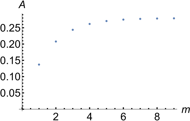
In Figure 1, we plot the average skew information-based coherence for random mixed states. The $A$-axis shows the value of $\mathbb{E}_{\rho}[C_{I}(\rho)]$ given by Eq.(19). Numerical calculations show that as the dimension $N$ increases, the expectation value $\mathbb{E}_{\rho}[C_{I}(\rho)]$ approaches to a number which is close to 0.28. Numerical computation shows that unlike the random pure states, for random mixed states, the average skew information-based coherence is closer to the minimal coherence 00 than the maximum coherence $1-\frac{1}{N}$.

Refer to caption
Figure 1: The average skew information-based coherence $A=\mathbb{E}_{\rho}[C_{I}(\rho)]$ as a function of $N=2^{m}$.

Based on the above result, we can similarly discuss the typicality of quantum coherence $C_{I}(\rho)$ for random mixed states.

Theorem 5 (Typicality of skew information-based coherence for random mixed states) Let $\rho_{A}\in\mathrm{D}(\mathbb{C}^{N})$ be a random mixed quantum state obtained via partial tracing over a Haar distributed pure state $|\psi\rangle_{AB}$ in $\mathbb{C}^{N}\otimes\mathbb{C}^{N}$. Then for all $\epsilon>0$, we have

$$\mathrm{Pr}\left\{\left|C_{I}(\rho_{A})-\mathbb{E}_{\rho}[C_{I}(\rho_{A})]\right|>\epsilon\right\}\leq 2\mathrm{exp}\left(-\frac{N\epsilon^{2}}{72\pi^{3}\mathrm{ln2}}\right),$$ (20)

where $\mathbb{E}_{\rho}[C_{I}(\rho_{A})]$ is given by Eq. (19).

Proof. Define the map $T:\mathbb{S}^{N^{2}}\mapsto\mathbb{R}$ as $T(\psi_{AB})=C_{I}(\rho_{A})$. Let $|\psi\rangle_{AB}=\sum_{k,l=1}^{N}\psi_{kl}|k\rangle_{A}|l\rangle_{B}$. Then $\rho_{A}=\sum_{k,k^{\prime}=1}^{N}p_{kk^{\prime}}|k\rangle_{A}\langle k^{\prime}|$, where $p_{kk^{\prime}}=\sum_{l=1}^{N}\psi_{kl}\overline{\psi_{k^{\prime}l}}$. For a bipartitie pure state $|\psi\rangle_{AB}$, it has been shown that $1-C_{I}(\psi_{AB})\leq[1-C_{I}(\rho_{A})][1-C_{I}(\rho_{B})]$ [14]. Since $0\leq C_{I}(\rho_{B})\leq 1-\frac{1}{N}$, we have $C_{I}(\rho_{A})\leq C_{I}(\psi_{AB})=1-\sum_{k,l=1}^{N}|\langle k\otimes l|\psi\rangle|^{4}=1-\sum_{k,l=1}^{N}|\psi_{kl}|^{4}$. Denote $\tilde{T}(\psi_{AB})=C_{I}(\psi_{AB})$. Noting that $p_{kk}=\sum_{l=1}^{N}|\psi_{kl}|^{2}$ with $\sum_{k=1}^{N}p_{kk}=1$, we have

$\displaystyle\eta^{2}:=\sup_{\langle\psi|\psi\rangle\leq 1}\nabla\tilde{T}\cdot\nabla\tilde{T}$ $\displaystyle=$ $\displaystyle\sup_{\langle\psi|\psi\rangle\leq 1}\sum_{k,l=1}^{N}(|\psi_{kl}|^{3})^{2}=\sup_{\langle\psi|\psi\rangle\leq 1}16\sum_{k,l=1}^{N}|\psi_{kl}|^{6}$ (21)
$\displaystyle=$ $\displaystyle\sup_{\langle\psi|\psi\rangle\leq 1}16\sum_{k,l=1}^{N}(|\psi_{kl}|^{2})^{3}$
$\displaystyle\leq$ $\displaystyle\sup_{\langle\psi|\psi\rangle\leq 1}16\left(\sum_{k,l=1}^{N}|\psi_{kl}|^{2}\right)^{3}=16,$

which implies that $\eta\leq 4$. Now, the Lipschitz constant for $T$ can be obtained in the following way. Suppose that $\sigma_{A}$ is the reduced state of another pure state $|\phi\rangle_{AB}$. Without loss of generality, assume that $C_{I}(\sigma_{A})\leq C_{I}(\rho_{A})$. We can choose $|\phi\rangle_{AB}$ such that $C_{I}(\sigma_{A})=C_{I}(\phi_{AB})$. Then

$$C_{I}(\rho_{A})-C_{I}(\sigma_{A})\leq C_{I}(\psi_{AB})-C_{I}(\phi_{AB})\leq\eta\||\psi\rangle_{AB}-|\phi\rangle_{AB}\|_{2},$$

Thus the Lipschitz constant of $T$ is bounded by that of $\tilde{T}$ and can be chosen to be $4$. This completes the proof. $\Box$

6. Conclusions and discussions

We have deduced the explicit formulae for the skew information-based coherence for both random pure states and random mixed states. It is found that as $N$ approaches to infinity, the limit of the average coherence for random pure states is $1$, while this limit for random mixed states is a positive constant less than $\frac{1}{2}$ by numerical computation. The average skew information-based coherence is always closer to the maximum coherence than the minimum coherence for random pure states, while it is always closer to the minimum coherence than the maximum coherence for random mixed states, which demonstrate that for a randomly-chosen state, a quantum pure state may give rise to more coherence as a resource compared with a quantum mixed one. This property coincides with the one when relative entropy of coherence is taken into consideration.

From Eq. (10) it is found that $0\leq\mathbb{E}_{\psi}[C_{I}(\psi)]\leq 1$, i.e., the average skew information-based coherence for a random pure state is always uniformly bounded, while the average relative entropy of coherence for a random pure state is $\mathbb{E}_{\psi}[C_{r}(\psi)]=H_{N}-1$ [61], which approaches to infinity as the dimension $N$ increases, where $H_{N}=\sum_{k=1}^{N}1/k$ is the $N$th harmonic number. Unlike a pure state, in [62], it is shown that the average relative entropy of coherence for a random mixed state is $\mathbb{E}_{\rho}[C_{r}(\rho)]=\frac{N-1}{2N}$. Combining this fact with the equality given in Eq. (19), we conclude that in the mixed state case, the average coherence for skew information-based coherence and relative entropy of coherence are both uniformly bounded. Also, it can be seen that $\mathbb{E}_{\psi}[C_{r}(\psi)]>\mathbb{E}_{\psi}[C_{I}(\psi)]$ and $\mathbb{E}_{\rho}[C_{r}(\rho)]>\mathbb{E}_{\rho}[C_{I}(\rho)]$, which implies that for both a random pure state and a random mixed state, more coherence as a resource could be generated when the relative entropy of coherence measure is utilized rather than the skew information-based one. Moreover, in random pure state case, it is interesting to note that for skew information-based coherence, the gap between the maximal coherence and the average coherence is $1-\frac{1}{N}-\frac{N-1}{N+1}=\frac{N-1}{N(N+1)}>0$, and the limit approaches to 00 as $N$ approaches to infinity, while for the relative entropy of coherence, it is found that this gap $\mathrm{ln}N-H_{N}+1\gg 0$.

Furthermore, we have shown that the average skew information-based coherence of pure quantum states (resp. mixed quantum states) sampled randomly from the uniform Haar measure is typical, i.e., the probability that the skew information-based coherence of a randomly chosen pure quantum state (resp. mixed quantum state) is not equal to the average relative entropy of coherence (within an arbitrarily small error) is exponentially small in the dimension of the Hilbert space.

We have also identified a coherent subspace, a large subspace of the Hilbert space such that the amount of the skew information-based coherence for each pure state in this subspace can be bounded from below almost always by a fixed number that is arbitrarily close to the typical value of coherence. The obtained results in this paper complement the corresponding results for relative entropy of coherence, and may shed new light on the study of quantum coherence from the probabilistic and statistical perspective.

Acknowledgements

The authors would like to thank the referees for their valuable comments, which greatly improved this paper. This work was supported by National Natural Science Foundation of China (Grant Nos. 11701259, 11971140, 11461045, 11675113), the China Scholarship Council (Grant No.201806825038), Natural Science Foundation of Jiangxi Province of China (Grant No. 20202BAB201001), the Key Project of Beijing Municipal Commission of Education (Grant No. KZ201810028042), Beijing Natural Science Foundation (Grant No. Z190005), Natural Science Foundation of Zhejiang Province of China (Grant No.LY17A010027). This work was completed while Zhaoqi Wu and Lin Zhang were visiting Max-Planck-Institute for Mathematics in the Sciences in Germany.

Appendix A: Proof of Lemma 1

Proof of Lemma 1. Note that $\prod_{1\leq i<j\leq N}(\mu_{i}-\mu_{j})$ is the classical Vandermonde determinant

$$\prod_{1\leq i<j\leq N}(\mu_{i}-\mu_{j})=\left|\begin{array}[]{ccc}1&\cdots&1\\ \mu_{1}&\cdots&\mu_{N}\\ \vdots&\ddots&\vdots\\ \mu_{1}^{N-1}&\cdots&\mu_{N}^{N-1}\\ \end{array}\right|.$$

It can be seen that if $P_{0},P_{1},\cdots,P_{N-1}$ are polynomials of respective degrees $0,1,\cdots,N-1$ and respective dominant coefficients $a_{0},a_{1},\cdots,a_{N-1}$, one has

$$\prod_{1\leq i<j\leq N}(\mu_{i}-\mu_{j})=\frac{1}{\prod_{k=0}^{N-1}a_{k}}\left|\begin{array}[]{ccc}P_{0}(\mu_{1})&\cdots&P_{0}(\mu_{N})\\ P_{1}(\mu_{1})&\cdots&P_{1}(\mu_{N})\\ \vdots&\ddots&\vdots\\ P_{N-1}(\mu_{1})&\cdots&P_{N-1}(\mu_{N})\\ \end{array}\right|$$

Now choose $P_{k}(x)$ to be Laguerre polynomials $L_{k}(x)$:

$$L_{k}(x)=\sum_{j=0}^{k}(-1)^{k}\tbinom{k}{k-j}\frac{x^{j}}{j!}.$$

Note that $L_{k}(x)$ have the orthogonality property

$$\int_{0}^{\infty}L_{k}(x)L_{l}(x)e^{-x}dx=\delta_{kl},$$ (22)

and the coefficient of the term with the highest degree is $a_{k}=\frac{(-1)^{k}}{k!}$. We have

$\displaystyle\prod_{1\leq i<j\leq N}(\mu_{i}-\mu_{j})^{2}$ $\displaystyle=$ $\displaystyle\frac{1}{\prod_{k=0}^{N-1}a_{k}^{2}}\left|\begin{array}[]{ccc}L_{0}(\mu_{1})&\cdots&L_{0}(\mu_{N})\\ L_{1}(\mu_{1})&\cdots&L_{1}(\mu_{N})\\ \vdots&\ddots&\vdots\\ L_{N-1}(\mu_{1})&\cdots&L_{N-1}(\mu_{N})\\ \end{array}\right|$ (27)
$\displaystyle=$ $\displaystyle\prod_{k=0}^{N-1}(k!)^{2}\sum_{\sigma,\tau\in S_{N}}\mathrm{sgn}(\sigma)\mathrm{sgn}(\tau)L_{\sigma(k)-1}(\mu_{k})L_{\tau(k)-1}(\mu_{k}),$ (28)

which implies that

$\displaystyle\int_{\mathbb{R}_{+}^{N}}\sqrt{\mu_{1}\mu_{2}}\mathrm{exp}\left(-\sum_{j=1}^{N}\mu_{j}\right)|\Delta(\mu)|^{2}\prod_{j=1}^{N}\mathrm{d}\mu_{j}$
$\displaystyle=\prod_{k=0}^{N-1}(k!)^{2}\sum_{\sigma,\tau\in S_{N}}\mathrm{sgn}(\sigma)\mathrm{sgn}(\tau)\left(\int_{0}^{\infty}\sqrt{\mu_{1}}e^{-\mu_{1}}L_{\sigma(1)-1}(\mu_{1})L_{\tau(1)-1}(\mu_{1})\mathrm{d}\mu_{1}\right)$
$\displaystyle\left(\int_{0}^{\infty}\sqrt{\mu_{2}}e^{-\mu_{2}}L_{\sigma(2)-1}(\mu_{2})L_{\tau(2)-1}(\mu_{1})\mathrm{d}\mu_{2}\right)\left(\prod_{k=3}^{N}\int_{\mathbb{R}_{+}^{N-2}}e^{-\mu_{k}}L_{\sigma(k)-1}(\mu_{k})L_{\tau(k)-1}(\mu_{k})\mathrm{d}\mu_{k}\right),$

where $S_{N}$ is the permutation group on $\{1,2,\cdots,N\}$.

Denote $I_{kl}^{(q)}:=\int_{0}^{\infty}L_{k}(x)L_{l}(x)e^{-x}x^{q}dx$, where $q>-1$. It holds that [52]

$$I_{kl}^{(q)}=\sum_{r=0}^{\min(k,l)}(-1)^{k+l}\tbinom{q}{k-r}\tbinom{q}{l-r}\frac{\Gamma(q+r+1)}{r!},~{}~{}q>-1.$$ (29)

Note that

$$\int_{0}^{\infty}\sqrt{\mu_{i}}e^{-\mu_{i}}L_{\sigma(i)-1}(\mu_{i})L_{\tau(i)-1}(\mu_{i})\mathrm{d}\mu_{i}=I_{\sigma(i)-1,\tau(i)-1}^{(\frac{1}{2})},~{}~{}i=1,2$$

and

$$\int_{0}^{\infty}\sqrt{\mu_{i}}e^{-\mu_{i}}L_{\sigma(1)-1}(\mu_{i})L_{\sigma(2)-1}(\mu_{i})\mathrm{d}\mu_{i}=I_{\sigma(1)-1,\sigma(2)-1}^{(\frac{1}{2})},~{}~{}i=1,2.$$

We calculate the integral $\int_{\mathbb{R}_{+}^{N}}\sqrt{\mu_{1}\mu_{2}}\mathrm{exp}\left(-\sum_{j=1}^{N}\mu_{j}\right)|\Delta(\mu)|^{2}\prod_{j=1}^{N}\mathrm{d}\mu_{j}$ by considering the following two cases.

Case I: $\sigma=\tau$. Denote $I=\sum_{k=0}^{N-1}I_{kk}^{(\frac{1}{2})}$, we have

$\displaystyle\sum_{\sigma,\tau\in S_{N},\sigma=\tau}\mathrm{sgn}(\sigma)\mathrm{sgn}(\tau)\left(\int_{0}^{\infty}\sqrt{\mu_{1}}e^{-\mu_{1}}L_{\sigma(1)-1}(\mu_{1})L_{\tau(1)-1}(\mu_{1})\mathrm{d}\mu_{1}\right)$
$\displaystyle\left(\int_{0}^{\infty}\sqrt{\mu_{2}}e^{-\mu_{2}}L_{\sigma(2)-1}(\mu_{2})L_{\tau(2)-1}(\mu_{1})\mathrm{d}\mu_{2}\right)\left(\prod_{k=3}^{N}\int_{\mathbb{R}_{+}^{N-2}}e^{-\mu_{k}}L_{\sigma(k)-1}(\mu_{k})L_{\tau(k)-1}(\mu_{k})\mathrm{d}\mu_{k}\right)$
$\displaystyle=\sum_{\sigma\in S_{N}}I_{\sigma(1)-1,\sigma(1)-1}^{(\frac{1}{2})}I_{\sigma(2)-1,\sigma(2)-1}^{(\frac{1}{2})}=(N-2)!\sum_{k\neq l}I_{kk}^{(\frac{1}{2})}I_{ll}^{(\frac{1}{2})}$
$\displaystyle=(N-2)!\left[\left(\sum_{k=0}^{N-1}I_{kk}^{(\frac{1}{2})}\right)^{2}-\sum_{k=0}^{N-1}\left(I_{kk}^{(\frac{1}{2})}\right)^{2}\right].$ (30)

Case II: $\sigma\neq\tau$. First, note that if there exists $k_{0}\in\{3,4,\cdots,N\}$ such that $\sigma(k_{0})\neq\tau(k_{0})$, then by Eq. (22) we have

$$\left(\prod_{k=3}^{N}\int_{\mathbb{R}_{+}^{N-2}}e^{-\mu_{k}}L_{\sigma(k)-1}(\mu_{k})L_{\tau(k)-1}(\mu_{k})\mathrm{d}\mu_{k}\right)=0.$$

Thus $\int_{\mathbb{R}_{+}^{N}}\sqrt{\mu_{1}\mu_{2}}\mathrm{exp}\left(-\sum_{j=1}^{N}\mu_{j}\right)|\Delta(\mu)|^{2}\prod_{j=1}^{N}\mathrm{d}\mu_{j}=0$. Otherwise, $\sigma(i)=\tau(i)$ for $i=3,\cdots,N$, which implies that $\sigma(1)=\tau(2)$ and $\sigma(2)=\tau(1)$, i.e., $\tau=\sigma(12)$. Then we have

$\displaystyle\sum_{\sigma,\tau\in S_{N},\sigma\neq\tau}\mathrm{sgn}(\sigma)\mathrm{sgn}(\tau)\left(\int_{0}^{\infty}\sqrt{\mu_{1}}e^{-\mu_{1}}L_{\sigma(1)-1}(\mu_{1})L_{\tau(1)-1}(\mu_{1})\mathrm{d}\mu_{1}\right)$
$\displaystyle\left(\int_{0}^{\infty}\sqrt{\mu_{2}}e^{-\mu_{2}}L_{\sigma(2)-1}(\mu_{2})L_{\tau(2)-1}(\mu_{1})\mathrm{d}\mu_{2}\right)\left(\prod_{k=3}^{N}\int_{\mathbb{R}_{+}^{N-2}}e^{-\mu_{k}}L_{\sigma(k)-1}(\mu_{k})L_{\tau(k)-1}(\mu_{k})\mathrm{d}\mu_{k}\right)$
$\displaystyle=\sum_{\sigma\in S_{N}}(-1)I_{\sigma(1)-1,\sigma(2)-1}^{(\frac{1}{2})}I_{\sigma(2)-1,\sigma(1)-1}^{(\frac{1}{2})}=-(N-2)!\sum_{k\neq l}(I_{kl}^{(\frac{1}{2})})^{2}.$ (31)

Combining Eqs. (Acknowledgements) and (Acknowledgements), we have

$\displaystyle\int_{\mathbb{R}_{+}^{N}}\sqrt{\mu_{1}\mu_{2}}\mathrm{exp}\left(-\sum_{j=1}^{N}\mu_{j}\right)|\Delta(\mu)|^{2}\prod_{j=1}^{N}\mathrm{d}\mu_{j}$
$\displaystyle=\prod_{k=0}^{N-1}(k!)^{2}\left[(N-2)!\left(\left(\sum_{k=0}^{N-1}I_{kk}^{(\frac{1}{2})}\right)^{2}-\sum_{k=0}^{N-1}\left(I_{kk}^{(\frac{1}{2})}\right)^{2}\right)-(N-2)!\sum_{k\neq l}\left(I_{kl}^{(\frac{1}{2})}\right)^{2}\right]$
$\displaystyle=(N-2)!\prod^{N}_{j=1}\Gamma(j)^{2}\left[\left(\sum_{k=0}^{N-1}I_{kk}^{(\frac{1}{2})}\right)^{2}-\sum_{k,l=0}^{N-1}\left(I_{kl}^{(\frac{1}{2})}\right)^{2}\right],$ (32)

where

$$I_{kl}^{(\frac{1}{2})}=\sum_{r=0}^{\min(k,l)}(-1)^{k+l}\tbinom{\frac{1}{2}}{k-r}\tbinom{\frac{1}{2}}{l-r}\frac{\Gamma(\frac{3}{2}+r)}{r!}.$$

$\Box$

Appendix B: Proof of Theorem 4

Proof of Theorem 4. Since $\mathrm{d\mu_{HS}}$ is a normalized Hilbert-Schmidt measure, by the definition of $C_{I}(\rho)$, we have

$\displaystyle\int_{\mathrm{D}(\mathbb{C}^{N})}C_{I}(\rho)\mathrm{d\mu_{HS}}(\rho)$ $\displaystyle=$ $\displaystyle\int_{\mathrm{D}(\mathbb{C}^{N})}\left[1-\sum_{k=1}^{N}\langle k|\sqrt{\rho}|k\rangle^{2}\right]\mathrm{d\mu_{HS}}(\rho)$ (33)
$\displaystyle=$ $\displaystyle 1-\int_{\mathrm{D}(\mathbb{C}^{N})}\sum_{k=1}^{N}\langle k^{\otimes 2}|\sqrt{\rho}^{\otimes 2}|k^{\otimes 2}\rangle\mathrm{d\mu_{HS}}(\rho)$
$\displaystyle=$ $\displaystyle 1-\sum_{k=1}^{N}\left\langle k^{\otimes 2}\left|\int_{\mathrm{D}(\mathbb{C}^{N})}\sqrt{\rho}^{\otimes 2}\mathrm{d\mu_{HS}}(\rho)\right|k^{\otimes 2}\right\rangle.$

It suffices to compute the integral $\int_{\mathrm{D}(\mathbb{C}^{N})}\sqrt{\rho}^{\otimes 2}\mathrm{d\mu_{HS}}(\rho).$ In fact, by the factorization in Eq. (7), it follows that

$\displaystyle\int_{\mathrm{D}(\mathbb{C}^{N})}\sqrt{\rho}^{\otimes 2}\mathrm{d\mu_{HS}}(\rho)$ (34)
$\displaystyle=\int\mathrm{d\nu(\Lambda)}\int_{\mathrm{U(N)}}\left[(U\otimes U)(\sqrt{\Lambda}\otimes\sqrt{\Lambda})(U\otimes U)^{{\dagger}}\mathrm{d\mu_{Haar}}(U)\right].$

Using the following formula for integral over unitary groups [75]:

$\displaystyle\int_{\mathrm{U(N)}}(U\otimes U)A(U\otimes U)^{{\dagger}}\mathrm{d\mu_{Haar}}(U)$
$\displaystyle=\left(\frac{\mathrm{Tr}(A)}{N^{2}-1}-\frac{\mathrm{Tr}(AF)}{N(N^{2}-1)}\right)\mathbf{1}_{N^{2}}-\left(\frac{\mathrm{Tr}(A)}{N(N^{2}-1)}-\frac{\mathrm{Tr}(AF)}{N^{2}-1}\right)F,$ (35)

where $A\in M_{N^{2}}(\mathbb{C})$ and $F$ is the swap operator defined by $F|ij\rangle=|ji\rangle$ for all $i,j=1,2,\cdots,N$, we have

$\displaystyle\int_{\mathrm{U(N)}}(U\otimes U)(\sqrt{\Lambda}\otimes\sqrt{\Lambda})(U\otimes U)^{{\dagger}}\mathrm{d\mu_{Haar}}(U)=\frac{N(\mathrm{Tr}\sqrt{\Lambda})^{2}-1}{N(N^{2}-1)}\mathbf{1}_{N^{2}}+\frac{N-(\mathrm{Tr}\sqrt{\Lambda})^{2}}{N(N^{2}-1)}F.$ (36)

Noting that

$\displaystyle\int(\mathrm{Tr}\sqrt{\Lambda})^{2}\mathrm{d\nu(\Lambda)}$ $\displaystyle=$ $\displaystyle\int\mathrm{d\nu(\Lambda)}+2\int\sum_{1\leq i<j\leq N}\sqrt{\lambda_{i}\lambda_{j}}\mathrm{d\nu(\Lambda)}$ (37)
$\displaystyle=$ $\displaystyle 1+2\int\sum_{1\leq i<j\leq N}\sqrt{\lambda_{i}\lambda_{j}}\mathrm{d\nu(\Lambda)}$
$\displaystyle=$ $\displaystyle 1+2C_{\mathrm{HS}}^{N}\int_{\mathbb{R}_{+}^{N}}\sum_{1\leq i<j\leq N}\sqrt{\lambda_{i}\lambda_{j}}\delta\left(1-\sum_{j=1}^{N}\lambda_{j}\right)|\Delta(\lambda)|^{2}\prod_{j=1}^{N}\mathrm{d}\lambda_{j}$
$\displaystyle=$ $\displaystyle 1+2C_{\mathrm{HS}}^{N}\tbinom{N}{2}\int_{\mathbb{R}_{+}^{N}}\sqrt{\lambda_{1}\lambda_{2}}\delta\left(1-\sum_{j=1}^{N}\lambda_{j}\right)|\Delta(\lambda)|^{2}\prod_{j=1}^{N}\mathrm{d}\lambda_{j},$

where $C_{\mathrm{HS}}^{N}$ is given in Eq. (9), we only need to calculate

$$\int_{\mathbb{R}_{+}^{N}}\sqrt{\lambda_{1}\lambda_{2}}\delta\left(1-\sum_{j=1}^{N}\lambda_{j}\right)|\Delta(\lambda)|^{2}\prod_{j=1}^{N}\mathrm{d}\lambda_{j}.$$

Denote

$$F(t)=\int_{\mathbb{R}_{+}^{N}}\sqrt{\lambda_{1}\lambda_{2}}\delta\left(t-\sum_{j=1}^{N}\lambda_{j}\right)|\Delta(\lambda)|^{2}\prod_{j=1}^{N}\mathrm{d}\lambda_{j}.$$

By performing Laplace transform $(t\rightarrow s)$ of $F(t)$, and letting $\mu_{j}=s\lambda_{j},j=1,2$, we get

$\displaystyle\tilde{F}(s)$ $\displaystyle=$ $\displaystyle\int_{\mathbb{R}_{+}^{N}}\sqrt{\lambda_{1}\lambda_{2}}\mathrm{exp}\left(-s\sum_{j=1}^{N}\lambda_{j}\right)|\Delta(\lambda)|^{2}\prod_{j=1}^{N}\mathrm{d}\lambda_{j}$ (38)
$\displaystyle=$ $\displaystyle s^{-(N^{2}+1)}\int_{\mathbb{R}_{+}^{N}}\sqrt{\mu_{1}\mu_{2}}\mathrm{exp}\left(-\sum_{j=1}^{N}\mu_{j}\right)|\Delta(\mu)|^{2}\prod_{j=1}^{N}\mathrm{d}\mu_{j}.$

Utilizing the inverse Laplace transform $(s\rightarrow t):\mathscr{L}^{-1}(s^{\alpha})=\frac{t^{-\alpha-1}}{\Gamma(-\alpha)}$, we obtain

$$F(t)=\frac{t^{N^{2}}}{\Gamma(N^{2}+1)}\int_{\mathbb{R}_{+}^{N}}\sqrt{\mu_{1}\mu_{2}}\mathrm{exp}\left(-\sum_{j=1}^{N}\mu_{j}\right)|\Delta(\mu)|^{2}\prod_{j=1}^{N}\mathrm{d}\mu_{j}.$$ (39)

Thus

$\displaystyle\int_{\mathbb{R}_{+}^{N}}\sqrt{\lambda_{1}\lambda_{2}}\delta\left(1-\sum_{j=1}^{N}\lambda_{j}\right)|\Delta(\lambda)|^{2}\prod_{j=1}^{N}\mathrm{d}\lambda_{j}$
$\displaystyle=\frac{1}{\Gamma(N^{2}+1)}\int_{\mathbb{R}_{+}^{N}}\sqrt{\mu_{1}\mu_{2}}\mathrm{exp}\left(-\sum_{j=1}^{N}\mu_{j}\right)|\Delta(\mu)|^{2}\prod_{j=1}^{N}\mathrm{d}\mu_{j}.$ (40)

Substituting Eq. (Average skew information-based coherence and its typicality for random quantum states) into Eq. (Acknowledgements) yields

$\displaystyle\int_{\mathbb{R}_{+}^{N}}\sqrt{\lambda_{1}\lambda_{2}}\delta\left(1-\sum_{j=1}^{N}\lambda_{j}\right)|\Delta(\lambda)|^{2}\prod_{j=1}^{N}\mathrm{d}\lambda_{j}$
$\displaystyle=\frac{(N-2)!\prod^{N}_{j=1}\Gamma(j)^{2}}{\Gamma(N^{2}+1)}\left[\left(\sum_{k=1}^{N}I_{kk}^{(\frac{1}{2})}\right)^{2}-\sum_{k,l=1}^{N}\left(I_{kl}^{(\frac{1}{2})}\right)^{2}\right],$ (41)

which by Eqs. (9) and (37) gives rise to

$\displaystyle\int(\mathrm{Tr}\sqrt{\Lambda})^{2}\mathrm{d\nu(\Lambda)}=1+\frac{1}{N^{2}}\left[\left(\sum_{k=1}^{N}I_{kk}^{(\frac{1}{2})}\right)^{2}-\sum_{k,l=1}^{N}\left(I_{kl}^{(\frac{1}{2})}\right)^{2}\right].$ (42)

Combining Eqs. (34), (36) and (42), we obtain

$\displaystyle\int_{\mathrm{D}(\mathbb{C}^{N})}\sqrt{\rho}^{\otimes 2}\mathrm{d\mu_{HS}}(\rho)$
$\displaystyle=\int\left[\frac{N(\mathrm{Tr}\sqrt{\Lambda})^{2}-1}{N(N^{2}-1)}\mathbf{1}_{N^{2}}+\frac{N-(\mathrm{Tr}\sqrt{\Lambda})^{2}}{N(N^{2}-1)}F\right]\mathrm{d\nu(\Lambda)}$
$\displaystyle=\frac{N\mathbf{1}_{N^{2}}-F}{N(N^{2}-1)}\int(\mathrm{Tr}\sqrt{\Lambda})^{2}\mathrm{d\nu(\Lambda)}+\frac{NF-\mathbf{1}_{N^{2}}}{N(N^{2}-1)}\int\mathrm{d\nu(\Lambda)}$
$\displaystyle=\frac{N\mathbf{1}_{N^{2}}-F}{N(N^{2}-1)}\left(1+\frac{1}{N^{2}}\left[\left(\sum_{k=1}^{N}I_{kk}^{(\frac{1}{2})}\right)^{2}-\sum_{k,l=1}^{N}\left(I_{kl}^{(\frac{1}{2})}\right)^{2}\right]\right)+\frac{NF-\mathbf{1}_{N^{2}}}{N(N^{2}-1)}.$

Finally, by using the fact that $\sum_{k=1}^{N}\langle k^{\otimes 2}|F|k^{\otimes 2}\rangle=N,$ we have

$$\sum_{k=1}^{N}\langle k^{\otimes 2}|N\mathbf{1}_{N^{2}}-F|k^{\otimes 2}\rangle=\sum_{k=1}^{N}\langle k^{\otimes 2}|NF-\mathbf{1}_{N^{2}}|k^{\otimes 2}\rangle=\frac{N^{2}-N}{N(N^{2}-1)}=\frac{1}{N+1}.$$

From Eq. (33) we get (19). $\Box$

References

  • [1] Streltsov A, Adesso G and Plenio M B 2017 Colloquium: Quantum coherence as a resource Rev. Mod. Phys. 89 041003
  • [2] Baumgratz T, Cramer M and Plenio M B 2014 Quantifying coherence Phys. Rev. Lett. 113 140401
  • [3] Napoli C, Bromley T R, Cianciaruso M, Piani M, Johnston N and Adesso G 2016 Robustness of Coherence: An operational and observable measure of quantum coherence Phys. Rev. Lett. 116 150502
  • [4] Bu K, Singh U, Fei S M, Pati A K and Wu J 2017 Maximum relative entropy of coherence: an operational coherence measure Phys. Rev. Lett. 119 150405
  • [5] Streltsov A, Singh U, Dhar H S, Bera M N and Adesso G 2015 Measuring quantum coherence with entanglement Phys. Rev. Lett. 115 020403
  • [6] Xiong C and Wu J 2018 Geometric coherence and quantum state discrimination J. Phys. A: Math. Theor. 51 414005
  • [7] Shao L H, Xi Z, Fan H and Li Y 2015 Fidelity and Trace-Norm Distances for Quantifying Coherence Phys. Rev. A 91 042120
  • [8] Rana S, Parashar P and Lewenstein M 2016 Trace-distance measure of coherence Phys. Rev. A 93 012110
  • [9] Yu X D, Zhang D J, Xu G F and Tong D M 2016 Alternative framework for quantifying coherence Phys. Rev. A 94 060302(R)
  • [10] Chen B and Fei S M 2018 Notes on modified trace distance measure of coherence Quantum Inf. Process. 17 107
  • [11] Girolami D 2014 Observable Measure of Quantum Coherence in Finite Dimensional Systems Phys. Rev. Lett. 113 170401
  • [12] Luo S and Sun Y 2017 Quantum coherence versus quantum uncertainty Phys. Rev. A 96 022130
  • [13] Luo S and Sun Y 2017 Partial coherence with application to the monotonicity problem of coherence involving skew information Phys. Rev. A 96 022136
  • [14] Yu C S 2017 Quantum coherence via skew information and its polygamy Phys. Rev. A 95 042337
  • [15] Luo S and Sun Y 2018 Coherence and complementarity in state-channel interaction Phys. Rev. A 98 012113
  • [16] Bu K, Anand N and Singh U 2018 Asymmetry and coherence weight of quantum states Phys. Rev. A 97 032342
  • [17] Xiong C, Kumar A and Wu J 2018 Family of coherence measure and duality between quantum coherence and path distinguishability Phys. Rev. A 98 032324
  • [18] Xiong C, Kumar A, Huang M, Das S, Sen U and Wu J 2019 Partial coherence and quantum correlation with fidelity and affinity distances Phys. Rev. A 99 032305
  • [19] Zhu X N, Jin Z X and Fei S M 2019 Quantifying quantum coherence based on the generalized $\alpha$-$z$-relative Rényi entropy Quantum Inf. Process. 18 179
  • [20] Xi Z and Yuwen S 2019 Coherence measure: Logarithmic coherence number Phys. Rev. A 99 022340
  • [21] Winter A and Yang D 2016 Operational resource theory of coherence Phys. Rev. Lett. 116 120404
  • [22] Chitambar E, Streltsov A, Rana S, Bera M N, Adesso G and Lewenstein M 2016 Assisted distillation of quantum coherence Phys. Rev. Lett. 116 070402
  • [23] Regula B, Fang K, Wang X and Adesso G 2018 One-shot coherence distillation Phys. Rev. Lett. 121 010401
  • [24] Zhao Q, Liu Y, Yuan X, Chitambar E and Winter A 2019 IEEE Trans. Inf. Theory 65 6441
  • [25] Fang K, Wang X, Lami L, Regula B and Adesso G 2018 Probabilistic distillation of quantum coherence Phys. Rev. Lett. 121 070404
  • [26] Liu C L and Zhou D L 2019 Deterministic coherence distillation Phys. Rev. Lett. 123 070402
  • [27] Lami L, Regula B and Adesso G 2019 Generic bound coherence under strictly incoherent operations Phys. Rev. Lett. 122 150402
  • [28] Zhao J M, Ma T, Quan Q, Fan H and Pereira R 2019 $l_{1}$-norm coherence of assistance Phys. Rev. A 100 012315
  • [29] Zhao Q, Liu Y, Yuan X, Chitambar E and Ma X 2018 One-shot coherence dilution Phys. Rev. Lett. 120 070403
  • [30] Lostaglio M and Müller M P 2019 Coherence and asymmetry cannot be broadcast Phys. Rev. Lett. 123 020403
  • [31] Marvian I and Spekkens R W 2019 No-broadcasting theorem for quantum asymmetry and coherence and a trade-off relation for approximate broadcasting Phys. Rev. Lett. 123 020404
  • [32] Chitambar E and Hsieh M H 2016 Relating the resource theories of entanglement and quantum coherence Phys. Rev. Lett. 117 020402
  • [33] Zhu H, Ma Z, Cao Z, Fei S M and Vedral V 2017 Operational one-to-one mapping between coherence and entanglement measures Phys. Rev. A 96 032316
  • [34] Xi Y, Zhang T , Zheng Z J, Li-Jost X and Fei S M 2019 Converting quantum coherence to genuine multipartite entanglement and nonlocality Phys. Rev. A 100 022310
  • [35] Ma J, Yadin B, Girolami D, Vedral V and Gu M 2016 Converting coherence to quantum correlations Phys. Rev. Lett. 116 160407
  • [36] Sun Y, Mao Y and Luo S 2017 From quantum coherence to quantum correlations Europhys. Lett. 118 60007
  • [37] Hu M L, Hu X, Wang J, Peng Y, Zhang X R and Fan H 2018 Quantum coherence and geometric quantum discord Phys. Rep. 762-764 1
  • [38] Kim S, Li L, Kumar A and Wu J 2018 Interrelation between partial coherence and quantum correlations Phys. Rev. A 98 022306 (2018).
  • [39] Wu K D, Hou Z, Zhao Y Y, Xiang G Y, Li C F, Guo G C, Ma J, He Q Y, Thompson J and Gu M 2018 Experimental cyclic interconversion between coherence and quantum correlations Phys. Rev. Lett. 121 050401
  • [40] Guo Z and Cao H 2019 Creating quantum correlation from coherence via incoherent quantum operations J. Phys. A: Math. Theor. 52 265301
  • [41] Bu K, Kumar A, Zhang L and Wu J 2017 Cohering power of quantum operations Phys. Lett. A 381 1670
  • [42] Du S, Bai Z and Qi X 2019 Coherence Manipulation under incoherent operations Phys. Rev. A 100 032313
  • [43] Wigner E P and Yanase M M 1963 Information contents of distributions Proc. Natl. Acad. Sci. USA 49 910
  • [44] Cheng S and Hall M J W 2015 Complementarity relations for quantum coherence Phys. Rev. A 92 042101
  • [45] Luo S and Sun Y 2019 Average versus maximal coherence Phys. Lett. A 383 2869
  • [46] Collins B and Nechita I 2016 Random matrix techniques in quantum information theory J. Math. Phys. 57 015215
  • [47] Ledoux M 2015 The Concentration of Measure Phenomenon (American Mathematical Society, Providence, RI)
  • [48] Hayden P, Leung D, Shor P W and Winter A 2004 Randomizing quantum states: Constructions and applications Commun. Math. Phys. 250 371
  • [49] Hayden P, Leung D W and Winter A 2006 Aspects of Generic Entanglement Commun. Math. Phys. 265 95
  • [50] Page D N 1993 Average entropy of a subsystem Phys. Rev. Lett. 71 1291
  • [51] Foong S K and Kanno S 1994 Proof of Page’s Conjecture on the average entropy of a subsystem Phys. Rev. Lett. 72 1148
  • [52] Sánchez-Ruiz J 1995 Simple proof of Page’s conjecture on the average entropy of a subsystem Phys. Rev. E 52 5653
  • [53] Sen S 1996 Average entropy of a quantum subsystem Phys. Rev. Lett. 77 1
  • [54] Malacarne L C, Mendes R S and Lenzi E K 2002 Average entropy of a subsystem from its average Tsallis entropy Phys. Rev. E 65 046131
  • [55] Datta A 2010 Negativity of random pure states Phys. Rev. A 81 052312
  • [56] Hamma A, Santra S and Zanardi P 2012 Quantum entanglement in random physical states Phys. Rev. Lett. 109 040502
  • [57] Dahlsten O C O, Lupo C, Mancini S and Serafini A 2014 Entanglement typicality J. Phys. A: Math. Theor. 47 363001
  • [58] Zhang L and Xiang H 2017 Average entropy of a subsystem over a global unitary orbit of a mixed bipartite state Quantum Inf. Process. 16 112
  • [59] Werner R F and Holevo A S 2002 Counterexample to an additivity conjecture for output purity of quantum channels J. Math. Phys. 43 4353
  • [60] Scott A J and Caves C M 2003 Entangling power of the quantum baker’s map J. Phys. A: Math. Gen. 36 9553
  • [61] Singh U, Zhang L and Pati A K 2016 Average coherence and its typicality for random pure states Phys. Rev. A 93 032125
  • [62] Zhang L 2017 Average coherence and its typicality for random mixed quantum states J. Phys. A: Math. Theor. 50 155303
  • [63] Zhang L, Singh U and Pati A K 2017 Average subentropy, coherence and entanglement of random mixed quantum states Ann. Phys. 377 125
  • [64] Zhang L and Wang J 2018 Average of uncertainty product for bounded observables Open Syst. Inf. Dyn. 25(2) 1850008
  • [65] Nielsen M A and Chuang I L 2000 Quantum Computation and Quantum Information (Cambridge University Press, Cambridge)
  • [66] Du S and Bai Z 2015 The Wigner-Yanase information can increase under phase sensitive incoherent operations Ann. Phys. (NY) 359 136
  • [67] Marvian I, Spekkens R W and Zanardi P 2016 Quantum speed limits, coherence and asymmetry Phys. Rev. A 93 052331
  • [68] ÓSearcóid M 2007 Metric Spaces (Springer-Verlag, London)
  • [69] Wilde M M 2013 Quantum Information Theory (Cambridge University Press, Cambridge, UK)
  • [70] Korn G A and Korn T M 2000 Mathematical Handbook for Scientists and Engineers: Definitions, Theorems, and Formulas for Reference and Review (Dover Publications, Dover)
  • [71] Bengtsson I and Życzkowski K 2017 Geometry of Quantum States: An Introduction to Quantum Entanglement 2nd ed (Cambridge University Press, Cambridge)
  • [72] Życzkowski K and Sommers H J 2001 Induced measures in the space of mixed quantum states J. Phys. A : Math. Gen. 34 7111
  • [73] Ginibre J 1965 Statistical ensembles of complex, quaternion, and real matrices J. Math. Phys. 6 440
  • [74] Mehta M 1991 Random Matrices 2nd ed (Academic Press, New York)
  • [75] Zhang L Matrix integrals over unitary groups: An application of Schur-Weyl duality arXiv:1408.3782