Dynamic Privacy Budget Allocation Improves Data Efficiency of Differentially Private Gradient Descent

Abstract.

Protecting privacy in learning while maintaining the model performance has become increasingly critical in many applications that involve sensitive data. Private Gradient Descent (PGD) is a commonly used private learning framework, which noises gradients based on the Differential Privacy protocol. Recent studies show that dynamic privacy schedules of decreasing noise magnitudes can improve loss at the final iteration, and yet theoretical understandings of the effectiveness of such schedules and their connections to optimization algorithms remain limited. In this paper, we provide comprehensive analysis of noise influence in dynamic privacy schedules to answer these critical questions. We first present a dynamic noise schedule minimizing the utility upper bound of PGD, and show how the noise influence from each optimization step collectively impacts utility of the final model. Our study also reveals how impacts from dynamic noise influence change when momentum is used. We empirically show the connection exists for general non-convex losses, and the influence is greatly impacted by the loss curvature.

1. Introduction

In the era of big data, privacy protection in machine learning systems is becoming a crucial topic as increasing personal data involved in training models (Dwork et al., 2020) and the presence of malicious attackers (Shokri et al., 2017; Fredrikson et al., 2015). In response to the growing demand, differential-private (DP) machine learning (Dwork et al., 2006) provides a computational framework for privacy protection and has been widely studied in various settings, including both convex and non-convex optimization (Wang et al., 2017; Wang et al., 2019; Jain et al., 2019).

One widely used procedure for privacy-preserving learning is the (Differentially) Private Gradient Descent (PGD) (Bassily et al., 2014; Abadi et al., 2016). A typical gradient descent procedure updates its model by gradients of the loss evaluated on a training dataset. When the data is sensitive, the gradients should be privatized to prevent excess privacy leakage. The PGD privatizes a gradient by adding controlled noise. As such, the models from PGD is expected to have a lower utility as compared to those from unprotected algorithms. In the cases where strict privacy control is exercised, or equivalently, a tight privacy budget, accumulating effects from highly-noised gradients may lead to unacceptable model performance. It is thus critical to design effective privatization procedures for PGD to maintain a great balance between utility and privacy.

Recent years witnessed a promising direction of privatization that dynamically allocate a privacy budget for each iteration to boost utility, under the constraint of a specified total privacy budget. One example is (Lee and Kifer, 2018), which reduces the budget-bonded noise magnitude when the loss does not decrease, due to the observation that gradients become very small when approaching convergence, and a static noise scale will overwhelm these gradients. Another example is (Yu et al., 2019), which periodically decreases the magnitude following a predefined strategy, e.g., exponential decaying or step decaying. Both approaches confirmed the empirically advantages of decreasing noise magnitudes. Intuitively, the dynamic mechanism may coordinate with certain properties of the learning task, e.g., training data and loss surface. Following the work, improved allocation policies are proposed, e.g., policies transferred from auxiliary datasets (Hong et al., 2021), policies with distributed budgets (Cheng et al., 2020), and a combination with adaptive learning rate (Xu et al., 2020). Yet there is little theoretical analysis available and two important questions remain unanswered: 1) What is the form of utility-preferred budget (or noise equivalently) schedules? 2) When and to what extent such an allocation policy improves utility?

Though there are theoretical studies of static-allocation policies, e.g., (Wang et al., 2017), the data efficiency is not the focus as discussions usually assume an unlimited amount of data is available. However, we argue that the data efficiency with limited data size is critical in practice, especially when DP makes the learning more data-hungry (McMahan et al., 2018). One example is federated learning (McMahan et al., 2017; McMahan et al., 2018), a distributed learning framework that aggregates many local models to form a stronger global model, where each model is privately trained on a local client, typically with very limited private data. Another example is biomedical applications, where collecting samples involves expansive clinical trials or cohort studies, resulting the scarcity of training set. To study biomarkers of Alzheimer’s, NIH has funded Alzheimer’s Disease Neuroimaging Initiative for $40 million, which collected imaging and genetic biomarkers from only 800 patients after 5 years’ extensive and collaborative efforts (Weiner et al., 2013). Therefore, we believe data efficiency needs to be taken into account in developing a private learning algorithm.

To answer these questions, in this paper we develop a principled approach to construct dynamic schedules and quantify their utility bounds in different learning algorithms. Our contributions are summarized as follows. 1) For the class of loss functions satisfying the Polyak-Lojasiewicz condition (Polyak, 1963), we show that dynamic schedules, that improve the utility upper bound with high data-efficiency, are shaped by the changing influence of per-iteration noise on the final loss. As the influence is tightly connected to the loss curvature, the advantage of using dynamic schedules therefore depends on the loss function. 2) Beyond vanilla gradient descent, our results show the gradient methods with momentum implicitly introduce a dynamic schedule and result in an non-monotonous influence trend. 3) We also show that our results are generalizable to population bounds in high probability or based on uniform stability theorems. Though our major focus is on the theoretic study, we empirically validate the results on a non-convex loss function formulated by a neural network. The empirical results suggest that a preferred dynamic schedule admits the exponentially decaying form, and works better when learning with high-curvature loss functions. Moreover, dynamic schedules give higher utility under stricter privacy conditions (e.g., smaller sample size and less privacy budget).

2. Related Work

Differentially Private Learning. Differential privacy (DP) characterizes the chance that an algorithm output (e.g., a learned model) leaks private information of its training data when the output distribution is known. Since outputs of many learning algorithms have undetermined distributions, the probabilistic risk is hard to measure. A common approach to tackle this issue is to inject randomness with known distribution to privatize the learning procedures. Classical methods include output perturbation (Chaudhuri et al., 2011), objective perturbation (Chaudhuri et al., 2011) and gradient perturbation (Abadi et al., 2016; Bassily et al., 2014; Wu et al., 2017). Among these approaches, the Private Gradient Descent (PGD) has attracted extensive attention in recent years because it can be flexibly integrated with variants of gradient-based iteration methods, e.g., stochastic gradient descent, momentum methods (Qian, 1999), and Adam (Kingma and Ba, 2015), for (non-)convex problems.

Dynamic Policies for Privacy Protection. Wang et al. (2017) studied the empirical risk minimization using dynamic variation reduction of perturbed gradients. They showed that the utility upper bound can be achieved by gradient methods under uniform noise parameters. Instead of enhancing the gradients, Yu et al. (2019); Lee and Kifer (2018) showed the benefits of using a dynamic schedule of privacy parameters or equivalently noise scales. Following (Lee and Kifer, 2018), a series of work (Cheng et al., 2020; Huang et al., 2019; Xie et al., 2021; Zhang et al., 2021) adaptively allocate privacy budget towards better privacy-utility trade-off. Moreover, adaptive sensitivity control (Pichapati et al., 2019; Thakkar et al., 2019) and dynamic batch sizes (Feldman et al., 2020) are also shown to improve convergence.

Table 1. Comparison of utility upper bound using different privacy schedules. The algorithms are $T$-iteration $\frac{1}{2}R$-zCDP under the PL condition (unless marked with * for convexity). The $O$ notation in this table drops other $\ln$ terms. Unless otherwise specified, all algorithms (including non-private GD) terminate at step $T={\mathcal{O}}(\ln{\frac{N^{2}R}{D}})$. Assume loss functions are $1$-smooth and $1$-Lipschitz continuous, and all parameters satisfy their numeric assumptions. Key notations: ${\mathcal{O}}_{p}$ – bound occurs in probability $p$; $D$ – feature dimension; $N$ – sample size; $R$ – privacy budget where $R_{\epsilon,\delta}$ is the equivalent budget accounted by $(\epsilon,\delta)$-DP; $c_{i}$ – constant; other notations can be found in Section 4. We provide citation after algorithm names for concise reference here and defer detailed explanations of baseline algorithms to Appendix B. Extensions to generalization error bounds are given in Table 2.

Algorithm	Schedule ($\sigma_{t}^{2}$)	Utility Upper Bound
*GD+Adv (Bassily et al., 2014)	${\mathcal{O}}\left({\ln(N/\delta)\over R_{\epsilon,\delta}}\right)$	${\mathcal{O}}\left(D\ln^{3}N\over NR_{\epsilon,\delta}\right)$
GD+MA (Wang et al., 2017)	${\mathcal{O}}({T\over R_{\epsilon,\delta}})$	${\mathcal{O}}\left({D\ln^{2}N\over N^{2}R_{\epsilon,\delta}}\right)$
GD+MA (adjusted utility) (Yu et al., 2020)	${\mathcal{O}}({T\over R_{\epsilon,\delta}})$	${\mathcal{O}}\left(\min{\sqrt{D}\over NR_{\epsilon,\delta}},{D\ln N\over N^{2}R^{2}_{\epsilon,\delta}}\right)$
GD+Adv+BBImp (Cummings et al., 2018)	${\mathcal{O}}\left({n^{2}\ln(n/\delta)\over R_{\epsilon,\delta}}\right)$	${\mathcal{O}}_{p}\left(D^{2}\ln^{2}(1/p)\over R_{\epsilon,\delta}N^{1-c}\right)$
Adam+MA (Zhou et al., 2020)	${\mathcal{O}}({T\over R_{\epsilon,\delta}})$	${\mathcal{O}}_{p}\left({\sqrt{D}\ln(ND\epsilon/(1-p))\over NR_{\epsilon,\delta}}\right)$
GD, Non-Private	$0$	${\mathcal{O}}\left(\frac{D}{N^{2}R}\right)$
GD+zCDP, Static Schedule	$\frac{T}{R}$	${\mathcal{O}}\left(\frac{D\ln N}{N^{2}R}\right)$
GD+zCDP, Dynamic Schedule	${\mathcal{O}}\left(\frac{\gamma^{(t-T)/2}}{R}\right)$	${\mathcal{O}}\left(\frac{D}{N^{2}R}\right)$
Momentum+zCDP, Static Schedule	$\frac{T}{R}$	${\mathcal{O}}\left(\frac{D}{N^{2}R}(c+\ln N\mathbb{I}_{T>\hat{T}})\right)$
Momentum+zCDP, Dynamic Schedule	${\mathcal{O}}\left({c_{1}\gamma^{T+t}+c_{2}\gamma^{(T-t)/2}\over R}\right)$	${\mathcal{O}}\left(\frac{D}{N^{2}R}(1+\frac{cD}{N^{2}R}\mathbb{I}_{T>\hat{T}})\right)$

Utility Upper Bounds. Utility upper bounds are a critical metric for privacy schedules, which characterizes the maximum utility that a schedule can deliver in theory. Wang et al. (2017) is the first to prove the utility bound under the PL condition. Recently, Zhou et al. proved the utility bound by using the momentum of gradients (Polyak, 1964; Kingma and Ba, 2015). In this paper, we improve the upper bound by a more accurate estimation of the dynamic influence of step noise. We show that introducing a dynamic schedule further boosts the sample-efficiency of the upper bound. Table 1 summarizes the upper bounds of a selection of state-of-the-art algorithms based on private gradients (up block, see Appendix B for the full list), and methods studied in this paper (down block), showing the benefits of dynamic influence.

Especially, a closely-related work by Feldman et al. achieved a convergence rate similar to ours in terms of generalization error bounds (c.f. SSGD in Table 2), by dynamically adjusting batch sizes (Feldman et al., 2020). However, the approach requires controllable batch sizes, which may not be feasible in many applications. In federated learning, for example, where users update models locally and then pass the parameters to server for aggregation, the server has no control over batch sizes, and coordinating users to use varying batch sizes may not be realistic. On the other hand, our proposed method can still be applied for enhancing utility, as the server can dynamically allocate privacy budget for each round when the presence of a user in the global aggregation is privatized (McMahan et al., 2018).

3. Private Gradient Descent

Notations. We consider a learning task by empirical risk minimization (ERM) $f(\theta)={1\over N}\sum_{n=1}^{N}f(\theta;x_{n})$ on a private dataset $\{x_{n}\}_{n=1}^{N}$ and $\theta\in\mathbb{R}^{D}$. The gradient methods are defined as $\theta_{t+1}=\theta_{t}-\eta_{t}\nabla_{t}$, where $\nabla_{t}=\nabla f(\theta_{t})={1\over N}\sum_{n}\nabla f(\theta_{t};x_{n})$ denotes the non-private gradient at iteration $t$, $\eta_{t}$ is the step learning rate. $\nabla_{t}^{(n)}=\nabla f(\theta_{t};x_{n})$ denotes the gradient on a sample $x_{n}$. $\mathbb{I}_{c}$ denotes the indicator function that returns $1$ if the condition $c$ holds, otherwise $0$.

Assumptions. (1) In this paper, we assume $f(\theta)$ is continuous and differentiable. Many commonly used loss functions satisfy this assumption, e.g., the logistic function. (2) For a learning task, only finite amount of privacy cost is allowed where the maximum cost is called privacy budget and denoted as $R$. (3) Generally, we assume that loss functions $f(\theta;x)$ (sample-wise loss) are $G$-Lipschitz continuous and $f(\theta)$ (the empirical loss) is $M$-smooth.

Definition 3.0 ($G$-Lipschitz continuity).

A function $f(\cdot)$ is $G$-Lipschitz continuous if, for $G>0$ and all $x,y$ in the domain of $f(\cdot)$, $f(\cdot)$ satisfies $\left\|f(y)-f(x)\right\|\leq G\left\|y-x\right\|$. .

Definition 3.0 ($m$-strongly convexity).

A function $f(\cdot)$ is $m$-strongly convex if $f(y)\geq f(x)+\nabla f(x)^{T}(y-x)+\frac{m}{2}\|y-x\|^{2}$, for some $m>0$ and all $x,y$ in the domain of $f(\cdot)$.

Definition 3.0 ($M$-smoothness).

A function is $M$-smooth w.r.t. $l_{2}$ norm if $f(y)\leq f(x)+\nabla f(x)^{T}(y-x)+\frac{M}{2}\|y-x\|^{2}$, for some constant $M>0$ and all $x,y$ in the domain of $f(\cdot)$.

For a private algorithm ${\mathcal{M}}(d)$ which maps a dataset $d$ to some output, the privacy cost is measured by the bound of the output difference on the adjacent datasets. Adjacent datasets are defined to be datasets that only differ in one sample. In this paper, we use the zero-Concentrated Differential Privacy (zCDP, see Definition 3.4) as the privacy measurement, because it provides the simplicity and possibility of adaptively composing privacy costs at each iteration. Various privacy metrics are discussed or reviewed in (Desfontaines and Pejó, 2019). A notable example is Moment Accoutant (MA) (Abadi et al., 2016), which adopts similar principle for composing privacy costs while is less tight for a smaller privacy budget. We note that alternative metrics can be adapted to our study without major impacts to the analysis.

Definition 3.0 ($\rho$-zCDP (Bun and Steinke, 2016)).

Let $\rho>0$. A randomized algorithm ${\mathcal{M}}:{\mathcal{D}}^{n}\rightarrow\mathbb{R}$ satisfies $\rho$-zCDP if, for all adjacent datasets $d,d^{\prime}\in{\mathcal{D}}^{n}$, $D_{\alpha}({\mathcal{M}}(d)\|{\mathcal{M}}(d^{\prime}))\leq\rho\alpha,~{}\forall\alpha\in(1,\infty)$ where $D_{\alpha}(\cdot\|\cdot)$ denotes the Rényi divergence (Rényi, 1961) of order $\alpha$.

The zCDP provides a linear composition of privacy costs of sub-route algorithms. When the input vector is privatized by injecting Gaussian noise of ${\mathcal{N}}(0,\sigma_{t}^{2}I)$ for the $t$-th iteration, the composed privacy cost is proportional to $\sum_{t}\rho_{t}$ where the step cost is $\rho_{t}={1\over\sigma_{t}^{2}}$. For simplicity, we absorb the constant coefficient into the (residual) privacy budget $R$. The formal theorems for the privacy cost computation of composition and Gaussian noising is included in Lemmas C.1 and C.3.

Input: Raw gradients $[\nabla_{t}^{(1)},\dots,\nabla_{t}^{(n)}]$ ($n=N$ by default), $v_{t}$, residual privacy budget $R_{t}$ assuming the full budget is $R$ and $R_{1}=R$.

1:$\rho_{t}\leftarrow 1/\sigma^{2}_{t}$, $\nabla_{t}\leftarrow{1\over n}\sum_{i=1}^{n}\nabla_{t}^{(i)}$ (Budget request)

2:if $\rho_{t}<R_{t}$ then

3:     $R_{t+1}\leftarrow R_{t}-\rho_{t}$

4:     $g_{t}\leftarrow\nabla_{t}+G\sigma_{t}\nu_{t}/N$, $\nu_{t}\sim\mathcal{N}(0,I)$ (Privacy noise)

5:     $m_{t+1}\leftarrow\phi(m_{t},g_{t})$ or $g_{1}$ if $t=1$

6:     return $\eta_{t}m_{t+1}$, $R_{t+1}$ (Utility projection)

7:else

8:     Terminate

Algorithm 1 Privatizing Gradients

Generally, we define the Private Gradient Descent (PGD) method as iterations for $t=1\dots T$:

(1) $$\theta_{t+1}=\theta_{t}-\eta_{t}\phi_{t}=\theta_{t}-\eta_{t}(\nabla_{t}+\sigma_{t}G\nu_{t}/N),$$

where $\phi_{t}=g_{t}$ is the gradient privatized from $\nabla_{t}$ as shown in Algorithm 1, $G/N$ is the bound of sensitivity of the gathered gradient excluding one sample gradient, and $\nu_{t}\sim\mathcal{N}(0,I)$ is a vector element-wisely subject to Gaussian distribution. We use $\sigma_{t}$ to denote the noise scale at step $t$ and use $\sigma$ to collectively represents the schedule $(\sigma_{1},\dots,\sigma_{T})$ if not confusing. When the Lipschitz constant is unknown, we can control the upper bound by scaling the gradient if it is over some constant. The scaling operation is often called clipping in literatures since it clips the gradient norm at a threshold. After the gradient is noised, we apply a modification, $\phi(\cdot)$, to enhance its utility. In this paper, we consider two types of $\phi(\cdot)$:

(2) $$\phi(m_{t},g_{t}) =g_{t}\text{ (GD)},$$

(3) $$~{}\phi(m_{t},g_{t}) =[\beta(1-\beta^{t-1})m_{t}+(1-\beta)g_{t}]/(1-\beta^{t})\text{ (Momentum)}$$

We now show that the PGD using Algorithm 1 guarantees a privacy cost less than $R$:

Theorem 3.5.

Suppose $f(\theta;x)$ is $G$-Lipschitz continuous and the PGD algorithm with privatized gradients defined by Algorithm 1, stops at step $T$. The PGD algorithm outputs $\theta_{T}$ and satisfies $\rho$-zCDP where $\rho\leq{1\over 2}R$.

Note that Theorem 3.5 allows $\sigma_{t}$ to be different throughout iterations. Next we present a principled approach for deriving dynamic schedules optimized for the final loss $f(\theta_{T})$.

4. Dynamic Policies by Minimizing Utility Upper Bounds

To characterize the utility of the PGD, we adopt the Expected Excess Risk (EER), which notion is widely used for analyzing the convergence of random algorithms, e.g., (Bassily et al., 2014; Wang et al., 2017). Due to the presence of the noise and the limitation of learning iterations, optimization using private gradients is expected to reach a point with a higher loss (i.e., excess risk) as compared to the optimal solution without private protection. Define $\theta^{*}=\operatorname*{arg\,min}\nolimits_{\theta}f(\theta)$, after Algorithm 1 is iterated for $T$ times in total, the EER gives the expected utility degradation:

$$\operatorname{EER}=\mathbb{E}_{\nu}[f(\theta_{T+1})]-f(\theta^{*}).$$

Due to the variety of loss function and complexity of recursive iterations, an exact EER with noise is intractable for most functions. Instead, we study the worst case scenario, i.e., the upper bound of the EER, and our goal is to minimize the upper bound. For consistency, we call the upper bound of EER divided by the initial error as ERUB. Since the analytical form of $\operatorname{EER}$ is either intractable or complicated due to the recursive iterations of noise, studying the $\operatorname{ERUB}$ is a convenient and tractable alternative. The upper bound often has convenient functional forms which are (1) sufficiently simple, such that we can directly minimize it, and (2) closely related to the landscape of the objective depending on both the training dataset and the loss function. As a consequence, it is also used in previous PGD literature (Pichapati et al., 2019; Wang et al., 2017) for choosing proper parameters. Moreover, we let $\operatorname{ERUB}_{\min}$ be the achievable optimal upper bound by a specific choice of parameters, e.g., the $\sigma$ and $T$.

As the EER is iteratively determined by Eq. 1, we define the influence of the dynamics in noise magnitude $\sigma_{t}$ as the derivative: $q_{t}^{*}=\frac{\partial\operatorname{EER}}{\partial\sigma_{t}}$. Accordingly, we can approximate the EER shift as $q_{t}^{*}\Delta\sigma_{t}$ when $\sigma_{t}$ increases by $\Delta\sigma_{t}$. However, because the EER is strongly data-dependent, the derived $q_{t}^{*}$ on a given dataset may not generalize to another dataset. Instead, we consider a more general term based on ERUB, i.e., $q_{t}=\frac{\partial\operatorname{ERUB}}{\partial\sigma_{t}}$.

In this paper, we consider the class of loss functions satisfying the Polyak-Lojasiewicz (PL) condition which bounds losses by corresponding gradient norms. It is more general than the $m$-strongly convexity. If $f$ is differentiable and $M$-smooth, then $m$-strongly convexity implies the PL condition.

Definition 4.0 (Polyak-Lojasiewicz condition (Polyak, 1963)).

For $f(\theta)$, there exists $\mu>0$ and for every $\theta$, $\left\|\nabla f(\theta)\right\|^{2}\geq 2\mu(f(\theta)-f(\theta^{*}))$.

The PL condition helps us to reveal how the influence of step noise propagates to the final excess error, i.e., EER. Though the assumption was also used previously in Wang et al. (2017); Zhou et al. (2020), neither did they discuss the propagated influence of noise. In the following sections, we will show how the influence can tighten the upper bound in gradient descent and its momentum variant.

4.1. Gradient Descent Methods and Noise Influences

For the brevity of variables, we first define the following summarized constants:

(4) non-private ERUB : $${\alpha}\triangleq{DG^{2}\over 2RMN^{2}(f(\theta_{1})-f(\theta^{*}))}\leq{\mathcal{O}}\left({DG^{2}\over RMN^{2}}\right),$$

(5) curvature : $$\kappa\triangleq{M\over\mu},$$

(6) convergence rate : $$\gamma\triangleq 1-{1\over\kappa},$$

which satisfy $\kappa\geq 1$ and $\gamma\in[0,1)$. Here, $\alpha$ is upper bounded by non-private ERUB within $T=\left\lceil{\mathcal{O}}(\ln{N^{2}R(M-\mu)\over DG^{2}})\right\rceil$ iterations. Therefore, $\alpha$ provide a simple reference of an ideal convergence bound, reaching which indicates a superior performance with privacy guarantee. $\kappa$ characterizes the curvature of $f(\cdot)$ which is the condition number of $f(\cdot)$ if $f(\cdot)$ is strongly convex, and $\gamma$ is the convergence rate for non-private SGD (c.f. Theorem 4.2 with $\sigma_{t}=0$). $\kappa$ tends to be large if the function is sensitive to small differences in inputs, and $1/\alpha$ tends to be large if more samples are provided and with a less strict privacy budget. The convergence of PGD under the PL condition has been studied for private (Wang et al., 2017) and non-private (Karimi et al., 2016; Nesterov and Polyak, 2006; Reddi et al., 2016) ERM. Below we extend the bound in (Wang et al., 2017) by considering dynamic influence of noise and relax $\sigma_{t}$ to be dynamic:

Theorem 4.2.

Let $\alpha$, $\kappa$ and $\gamma$ be defined in Eq. 6, and $\eta_{t}={1\over M}$. Suppose $f(\theta;x_{i})$ is $G$-Lipschitz and $f(\theta)$ is $M$-smooth satisfying the Polyak-Lojasiewicz condition. For PGD, the following holds:

(7) $$\operatorname{ERUB}=\gamma^{T}+R\sum\nolimits_{t=1}^{T}q_{t}\sigma_{t}^{2},\text{ where }q_{t}\triangleq\gamma^{T-t}\alpha.$$

Theorem 4.2 degenerates to a non-private variant as no noise is applied, i.e., $\sigma_{t}=0$ for all $t$. In Eq. 7, the step noise magnitude $\sigma_{t}^{2}$ has an exponential influence, $q_{t}$, on the EER. Note we ignore the constant factor $R$ in the influence. The Eq. 7 implies that the influence of noise at step $t$ increase quickly by an exponential rate. Importantly, the increasing rate is the same as the convergence rate, i.e., the first term in Eq. 7. The dynamic characteristic of the influence is the key to prove a tighter bound. Plus, on the presence of the dynamic influence, it is natural to choose a dynamic $\sigma_{t}^{2}$. When relaxing $q_{t}$ to a static $1$, a static $\sigma_{t}^{2}$ was studied by Wang et al. They proved a bound which is nearly optimal except a $\ln^{2}N$ factor. To get the optimal bound, in the following sections, we look for the $\sigma$ and $T$ that minimize the upper bound.

4.1.1. Uniform Schedule

The uniform setting of $\sigma_{t}$ has been previously studied in Wang et al. (2017). Here, we show that the bound can be further tightened by considering the dynamic influence of iterations and a proper $T$.

Theorem 4.3.

Suppose conditions in Theorem 4.2 are satisfied. When $\sigma_{t}^{2}=T/R$, let $\alpha$, $\gamma$ and $\kappa$ be defined in Eq. 6 and let $T$ be: $T=\left\lceil{\mathcal{O}}\left(\kappa\ln\left(1+{1\over\kappa\alpha}\right)\right)\right\rceil$. Meanwhile, if $\kappa\geq{1\over 1-c}>1$, $1/\alpha>1/\alpha_{0}$ for some constant $c\in(0,1)$ and $\alpha_{0}>0$, the corresponding bound is:

(8) $$\operatorname{ERUB}^{\text{uniform}}_{\min}=\Theta\left({\kappa^{2}\over\kappa+1/\alpha}\ln\left(1+{1\over\kappa\alpha}\right)\right).$$

Sketch of proof.

The key of proof is to find a proper $T$ to minimize

$$\operatorname{ERUB} =E=\gamma^{T}+\sum\nolimits_{t=1}^{T}\gamma^{T-t}\alpha R\sigma^{2}$$

(9) $$=\gamma^{T}+\alpha T{1-\gamma^{T}\over 1-\gamma}=\gamma^{T}+\alpha\kappa(1-\gamma^{T})T$$

where we use $\sigma_{t}=\sqrt{T/R}$. Vanishing its gradient is to solve $\gamma^{T}\ln\gamma+\alpha\kappa(1-\gamma^{T})-\alpha\kappa T\gamma^{T}\ln\gamma=0$, which however is intractable. In (Wang et al., 2017), $T$ is chosen to be ${\mathcal{O}}(\ln(1/\alpha))$ and ERUB is relaxed as $\gamma^{T}+\alpha\kappa T^{2}$. The approximation results in a less tight bound as ${\mathcal{O}}(\alpha(1+\kappa\ln^{2}(1/\alpha)))$ which explodes as $\kappa\rightarrow\infty$.

We observe that for a super sharp loss function, i.e., a large $\kappa$, any minor perturbation may result in tremendously fluctuating loss values. In this case, not-stepping-forward will be a good choice. Thus, we choose $T={1\over\ln(1/\gamma)}\ln\left(1+{\ln(1/\gamma)\over\alpha}\right)\leq{\mathcal{O}}\left(\kappa\ln\left(1+{1\over\kappa\alpha}\right)\right)$ which converges to $0$ as $\kappa\rightarrow+\infty$. The full proof is deferred to the appendix. ∎

4.1.2. Dynamic Schedule

A dynamic schedule can improve the upper bound delivered by the uniform schedule. First, we observe that the excess risk in Eq. 7 is upper bounded by two terms: the first term characterizes the error due to the finite iterations of gradient descents; the second term, a weighted sum, comes from error propagated from noise at each iteration. Now we show for any $\{q_{t}|q_{t}>0,t=1,\dots,T\}$ (not limited to the $q_{t}$ defined in Eq. 7), there is a unique $\sigma_{t}$ minimizing the weighted sum:

Lemma 4.4 (Dynamic schedule).

Suppose $\sigma_{t}$ satisfy $\sum_{t=1}^{T}\sigma_{t}^{-2}=R$. Given a positive sequence $\{q_{t}\}$, the following equation holds:

(10) $$\min_{\sigma}R\sum\nolimits_{t=1}^{T}q_{t}\sigma_{t}^{2} =\left(\sum\nolimits_{t=1}^{T}\sqrt{q_{t}}\right)^{2},\text{ when }\sigma_{t}^{2}={1\over R}\sum\nolimits_{i=1}^{T}\sqrt{q_{i}\over q_{t}}.$$

Remarkably, the difference between the minimum and $T\sum_{t=1}^{T}q_{t}$ (uniform $\sigma_{t}$) monotonically increases by the variance of $\sqrt{q_{t}}$ w.r.t. $t$.

We see that the dynamics in $\sigma_{t}$ come from the non-uniform nature of the weight $q_{t}$. Since $q_{t}$ presents the impact of the $\sigma_{t}$ on the final error, we denote it as influence. Given the dynamic schedule in Eq. 10, it is of our interest to which extent the ERUB can be improved. First, we present Theorem 4.5 to show the optimal $T$ and ERUB.

Theorem 4.5.

Suppose conditions in Theorem 4.2 are satisfied. Let $\alpha$, $\kappa$ and $\gamma$ be defined in Eq. 6. When $\eta_{t}={1\over M}$, $\sigma_{t}$ (based on Eqs. 7 and 10) and the $T$ minimizing ERUB are, i.e., $\sigma_{t}^{2}={1\over R}{\sqrt{(1/\gamma)^{T}}-1\over 1-\sqrt{\gamma}}\sqrt{\gamma^{t}}$, $T=\left\lceil\left({2\kappa}\ln\left(1+{1\over\kappa\alpha}\right)\right)\right\rceil$. Meanwhile, when $\kappa\geq 1$ and $1/\alpha\geq 1/\alpha_{0}$ for some positive constant $\alpha_{0}$, the minimal bound is:

(11) $$\operatorname{ERUB}^{\text{dynamic}}_{\min} =\Theta\left({\kappa^{2}\over\kappa^{2}+1/\alpha}\right).$$

4.1.3. Discussion

In Theorems 4.3 and 4.5, we present the tightest bounds for functions satisfying the PL condition, to our best knowledge. We further analyze the advantages of our bounds from two aspects: sample efficiency and robustness to sharp losses.

Sample efficiency. Since dataset cannot be infinitely large, it is critical to know how accurate the model can be trained privately with a limited number of samples. Formally, it is of interest to study when $\kappa$ is fixed and $N$ is large enough such that $\alpha\gg 1$. Then we have the upper bound in Eq. 8 as

(12) $$\operatorname{ERUB}^{\text{uniform}}_{\min}\leq{\mathcal{O}}\left({\kappa^{2}\alpha}\ln\left({1\over\kappa\alpha}\right)\right)\leq\tilde{\mathcal{O}}\left({DG^{2}\ln(N)\over MN^{2}R}\right),$$

where we ignore $\kappa$ and other logarithmic constants with $\tilde{\mathcal{O}}$ as done in Wang et al. (2017). As a result, we get a bound very similar to (Wang et al., 2017), except that $R$ is replaced by $R_{MA}=\epsilon^{2}/\ln(1/\delta)$ using Moment Accountant. In comparison, based on Lemma C.4, $R=2\rho=2\epsilon+4\ln(1/\delta)+4\sqrt{\ln(1/\delta)(\epsilon+\ln(1/\delta)}$ if $\theta_{T}$ satisfies $\rho$-zCDP. Because $\ln(1/\delta)>1$, it is easy to see $R=R_{zCDP}>R_{MA}$ when $\epsilon\leq 2\ln(1/\delta)$. As compared to the one reported in (Wang et al., 2017), our bound saved a factor of $\ln N$ and thus require less sample to achieve the same accuracy. Remarkably, the saving is due to the maintaining of the influence terms as shown in the proof of Theorem 4.3.

Using the dynamic schedule, we have $\operatorname{ERUB}^{\text{dynamic}}_{\min}\leq{\mathcal{O}}(\alpha)={\mathcal{O}}\left({DG^{2}\over MN^{2}R}\right)$, which saved another $\ln N$ factor in comparison to the one using the uniform schedule Eq. 12. As shown in Table 1, such advantage maintains when comparing with other baselines and reaches the ideal non-private case , recalling the meaning of $\alpha$.

Stability on ill-conditioned loss. Besides sample efficiency, we are also interested in robustness of the convergence under the presence of privacy noise. Because of the privacy noise, the private gradient descent will be unable to converge to where a non-private algorithm can reach. Specifically, when the samples are noisy or have noisy labels, the loss curvature may be sharp. The sharpness also implies lower smoothness, i.e., a small $M$ or has a very small PL parameter. Thus, gradients may change tremendously at some steps especially in the presence of privacy noise. Such changes have more critical impact when only a less number of iterations can be executed due to the privacy constraint. Assume $\alpha$ is some constant while $\kappa\gg 1/\alpha$, we immediately get:

$$\operatorname{ERUB}^{\text{uniform}}_{\min} =\Theta\left(\kappa\ln\left(1+{1\over\kappa\alpha}\right)\right)=\Theta\left({1\over\alpha}\right)\leq{\mathcal{O}}\left({MN^{2}R\over DG^{2}}\right),$$

$$~{}\operatorname{ERUB}^{\text{dynamic}}_{\min} =\Theta(1).$$

Both are robust, but the dynamic schedule has a smaller factor since $1/\alpha$ could be a large number. In addition, the factor implies that when more samples are used, the dynamic schedule is more robust.

4.2. Gradient Descent Methods with Momentum

Section 4.1 shows that the step noise has an exponentially increasing influence on the final loss, and therefore a decreasing noise magnitude improves the utility upper bound by a $\ln N$ factor. However, the proper schedule can be hard to find when the curvature information, e.g., $\kappa$, is absent. A parameterized method that less depends on the curvature information is preferred. On the other hand, long-term iterations will result in forgetting of the initial iterations, since accumulated noise overwhelmed the propagated information from the beginning. This effect will reduce the efficiency of the recursive learning frameworks.

Alternative to GD, the momentum method can mitigate the two issues. It was originally proposed to stabilize the gradient estimation (Polyak, 1964). In this section, we show that momentum (agnostic about the curvature) can flatten the dynamic influence and improve the utility upper bound. Previously, Pichapati et al. used the momentum as an estimation of gradient mean, without discussions of convergence improvements. Zhou et al. gave a bound for the Adam with DP. However, the derivation is based on gradient norm, which results in a looser bound (see Table 1).

The momentum method stabilizes gradients by moving average history coordinate values and thus greatly reduces the variance. The $\phi(m_{t},g_{t})$ can be rewritten as:

$$m_{t+1} =\phi(m_{t},g_{t})={v_{t+1}\over 1-\beta^{t}},$$

(13) $$v_{t+1} ={\beta v_{t}+(1-\beta)g_{t}}=(1-\beta)\sum\nolimits_{i=1}^{t}\beta^{t-i}g_{t},~{}v_{1}=0,$$

where $\beta\in[0,1]$. Note $v_{t+1}$ is a biased estimation of the gradient expectation while $m_{t+1}$ is unbiased.

Theorem 4.6 (Convergence under PL condition).

Suppose $f(\theta;x_{i})$ is $G$-Lipschitz, and $f(\theta)$ is $M$-smooth and satisfies the Polyak-Lojasiewicz condition. Assume $\beta\neq\gamma$ and $\beta\in(0,1)$. Let $\eta_{t}={\eta_{0}\over 2M}$ and $\eta_{0}\leq 8\left(\sqrt{1+{64\beta\gamma(\gamma-\beta)^{-2}(1-\beta)^{-3}}}+1\right)^{-1}$. Then the following holds:

$$\operatorname{EER}\leq\big{(}\gamma^{T}+2R\eta_{0}\alpha\underbrace{U_{3}(\sigma,T)}_{\text{noise varinace}}\big{)}(f(\theta_{1})-f(\theta^{*}))$$

(14) $$-\zeta{\eta_{0}\over 2M}\underbrace{\sum\nolimits_{t=1}^{T}\gamma^{T-t}\mathbb{E}\left\|v_{t+1}\right\|^{2}}_{\text{momentum effect}}$$

where $\gamma=1-{\eta_{0}\over\kappa}$, $\zeta=1-{1\over\beta(1-\beta)^{3}}\eta_{0}^{2}-{1\over 4}\eta_{0}\geq 0$, and $U_{3}=\sum\nolimits_{t=1}^{T}\gamma^{T-t}{(1-\beta)^{2}\over(1-\beta^{t})^{2}}\sum\nolimits_{i=1}^{t}\beta^{2(t-i)}\sigma_{i}^{2}$.

The upper bound includes three parts that influence the bound differently: (1) Convergence. The convergence term is mainly determined by $\eta_{0}$ and $\kappa$. $\eta_{0}$ should be in $(0,\kappa)$ such that the upper bound can converge. A large $\eta_{0}$ will be preferred to speed up convergence if it does not make the other two terms worse. (2) Noise Variance. The second term compressed in $U_{3}$ is the effect of the averaged noise, $\sum\nolimits_{i=1}^{t}\beta^{2(t-i)}\sigma_{i}^{2}$. One difference introduced by the momentum is the factor $(1-\beta)/(1-\beta^{t})$ which is less than $\gamma^{t}$ at the beginning and converges to a non-zero constant $1-\beta$. Therefore, in $U_{3}$, $\gamma^{T-t}(1-\beta)/(1-\beta^{t})$ will be constantly less than $\gamma^{T}$ meanwhile. Furthermore, when $t>\hat{T}$, the moving average $\sum\nolimits_{i=1}^{t}\beta^{2(t-i)}\sigma_{i}^{2}$ smooths the influence of each $\sigma_{t}$. (3) Momentum Effect. The momentum effect term can improve the upper bound when $\eta_{0}$ is small. For example, when $\beta=0.9$ and $\gamma=0.99$, then $\eta_{0}\leq 0.98/M$ which is a rational value. Following the analysis, when $M$ is large which means the gradient norms will significantly fluctuate, the momentum term may take the lead. Adjusting the noise scale in this case may be less useful for improving utility.

To give an insight on the effect of dynamic schedule, we provide the following utility bounds.

Theorem 4.7 (Uniform schedule).

Suppose the assumptions in Theorem 4.6 are satisfied. Let $\sigma_{t}^{2}=T/R$, and let: $\hat{T}=\max t~{}{\text{s.t.}}~{}\gamma^{t-1}\geq{1-\beta\over 1-\beta^{t}},~{}T=\left\lceil{\mathcal{O}}\left({\kappa\over\eta_{0}}\ln\left(1+{\eta_{0}\over\kappa\alpha}\right)\right)\right\rceil$. Given some positive constant $c$ and $\alpha_{0}>0$ with $1/\alpha>1/\alpha_{0}$, the following inequality holds:

$$\operatorname{ERUB}_{\min}\leq{\mathcal{O}}\left({\kappa^{2}\over\kappa+\eta_{0}/\alpha}\left[\mathbb{I}_{T\leq\hat{T}}+\gamma^{\hat{T}-1}\ln\left(1+{\eta_{0}\over\kappa\alpha}\right)\mathbb{I}_{T>\hat{T}}\right]\right).$$

Theorem 4.8 (Dynamic schedule).

Suppose the assumptions in Theorem 4.6 are satisfied. Let $\alpha^{\prime}={2\eta_{0}\alpha\over\gamma(1-\gamma\beta^{2})}$, $\beta<\gamma$ and $\hat{T}=\max t~{}{\text{s.t.}}~{}\gamma^{t-1}\geq{1-\beta\over 1-\beta^{t}}$. Use the following schedule: $\sigma_{t}^{2}={1\over R}\sum\nolimits_{i=1}^{T}\sqrt{q_{i}\over q_{t}},~{}T^{\text{dyn}}=\left\lceil{\mathcal{O}}\left({2\kappa\over\eta_{0}}\ln\left(1+{\eta_{0}\over\kappa\alpha}\right)\right)\right\rceil,$ where $q_{t}=c_{1}\gamma^{T+t}\mathbb{I}_{T\leq\hat{T}}+\gamma^{\hat{T}-1}c_{2}\gamma^{T-t}\mathbb{I}_{T>\hat{T}}$ for some positive constants $c_{1}$ and $c_{2}$. The following inequality holds:

$$\operatorname{ERUB} \leq\gamma^{T}+2\eta_{0}\alpha\sum\nolimits_{t=1}^{T}Rq_{t}\sigma_{t}^{2},$$

$$~{}\operatorname{ERUB}_{\min} \leq{\mathcal{O}}\left({\kappa\alpha\over\kappa\alpha+\eta_{0}}\left({\kappa\alpha\over\kappa\alpha+\eta_{0}}\mathbb{I}_{T\leq\hat{T}}+\mathbb{I}_{T>\hat{T}}\right)\right).$$

Discussion. Theoretically, the dynamic schedule is more influential in vanilla gradient descent methods than the momentum variant. The result is mainly attributed to the averaging operation. The moving averaging, $(1-\beta)\sum_{i=1}^{t}\beta^{t-i}g_{i}/(1-\beta^{t})$, increase the influence of the under-presented initial steps and decrease the one of the over-sensitive last steps. Counterintuitively, the preferred dynamic schedule should be increasing since $q_{t}$ decreases when $t\leq\hat{T}$.

4.3. Extension to Private Stochastic Gradient Descent

Though PGD provides a guarantee both for utility and privacy, computing gradients of the whole dataset is impractical for large-scale problems. For this sake, studying the convergence of Private Stochastic Gradient Descent (PSGD) is meaningful. The Algorithm 1 can be easily extended to PSGD by subsampling $n$ gradients where the batch size $n\ll N$. According to (Yu et al., 2019), when privacy is measured by zCDP, there are two ways to account for the privacy cost of PSGD depending on the batch-sampling method: sub-sampling with or without replacement. In this paper, we focus on the random subsampling with replacement since it is widely used in deep learning in literature, e.g., (Abadi et al., 2016; Feldman et al., 2020). Accordingly, we replace $N$ in the definition of $\alpha$ by $n$ because the term is from the sensitivity of batch data (see Eq. 1). For clarity, we assume that $T$ is the number of iterations rather than epochs and that $\tilde{\nabla}_{t}$ is mean stochastic gradient.

When a batch of data are randomly sampled, the privacy cost of one iteration is $cp^{2}{/\sigma_{t}}$ where $c$ is some constant, $p=n/N$ is the sample rate, and ${1/\sigma_{t}^{2}}$ is the full-batch privacy cost. Details of the sub-sampling theorems are referred to the Theorem 3 of (Yu et al., 2019) and their empirical setting. Threfore, we can replace the privacy constraint $\sum_{t}p^{2}/\sigma_{t}^{2}=R$ by $\sum_{t}{1/\sigma_{t}^{2}}=R^{\prime}$ where $R^{\prime}=R/p^{2}={N^{2}\over n^{2}}R$. Remarkably, we omit the constant $c$ because it will not affect the results regarding uniform or dynamic schedules. Notice $N^{2}R$ in the $\alpha$ is replaced by $n^{2}R^{\prime}=N^{2}R$. Thus, the form of $\alpha$ is not changed which provides convenience for the following derivations.

Now we study the utility bound of PSGD. To quantify the randomness of batch sampling, we define a random vector $\xi_{t}$ with $\mathbb{E}[\xi_{t}]=0$ and $\mathbb{E}\left\|\xi_{t}\right\|^{2}\leq D$ such that $\tilde{\nabla}_{t}\leq\nabla_{t}+\sigma_{g}\xi_{t}/n$ for some positive constant $\sigma_{g}$. Because $\xi_{t}$ has similar property to the privacy noise $\nu_{t}$, we can easily extend the PGD bounds to PSGD bounds by following theories.

Theorem 4.9 (Utility bounds of PSGD).

Let $\alpha$, $\kappa$ and $\gamma$ be defined in Eq. 6, and $\eta_{t}={1\over M}$. Suppose $f(\theta;x_{i})$ is $G$-Lipschitz and $f(\theta)$ is $M$-smooth satisfying the Polyak-Lojasiewicz condition. For PSGD, when batch size satisfies $n=\max\{N\sqrt{R},1\}$, the following holds: $\operatorname{ERUB}=\gamma^{T}+\alpha_{g}\sigma_{g}^{2}+R^{\prime}\sum\nolimits_{t=1}^{T}q_{t}\sigma_{t}^{2},\text{ where }q_{t}\triangleq\gamma^{T-t}\alpha,~{}\sum_{t}{1/\sigma_{t}^{2}}=R^{\prime}.$ where $\alpha_{g}={D\over 2\mu N^{2}R(f(\theta_{1})-f(\theta^{*}))}$.

Theorem 4.10 (PSGD with momentum).

Let $\alpha_{g}={D\over 2\mu N^{2}R(f(\theta_{1})-f(\theta^{*}))}$. Suppose assumptions in Theorem 4.6 holds. When batch size satisfies $n=\max\{N\sqrt{R},1\}$, the $U_{3}(\sigma,T)$ has to be replaced by $\tilde{U}_{3}=U_{3}^{g}+U_{3},\text{ with }\alpha R^{\prime}U_{3}^{g}\leq\alpha_{g}\sigma_{g}^{2}$ when PSGD is used.

As shown above, the utility bound of PSGD differs from the PGD merely by $\alpha_{g}\sigma_{g}^{2}$. Note $\alpha_{g}={\mathcal{O}}({D\over N^{2}R})$ which fits the order of dynamic-schedule bounds. In addition, $\alpha$ and other variables are not changed. Hence, the conclusions w.r.t. the dynamic/uniform schedules maintain the same.

4.4. Comaprison of generalization bounds

Table 2. Comparison of true excess risk bounds. The algorithms are $T$-iteration $\frac{1}{2}R$-zCDP or equivalently $(\epsilon,\delta)$-DP under the $\mu$-strongly-convex condition. The ${\mathcal{O}}$ notation in this table drops other $\ln$ terms. Assume loss functions are $1$-smooth and $1$-Lipschitz continuous, and all parameters satisfy their numeric assumptions. * marks the method with convex assumption.

Algorithm	Utility Upper Bd.	T
GD+Adv (Bassily et al., 2014)	${\mathcal{O}}_{1-p}\left(\sqrt{D}\ln^{2}N\ln(1/p)\over p\mu NR_{\epsilon,\delta}\right)$	${\mathcal{O}}(N^{2})$
SVRG+MA (Wang et al., 2017)	${\mathcal{O}}\left({D\ln N\over\mu N^{2}R_{\epsilon,\delta}}\right)$	${\mathcal{O}}(\ln{N^{2}R_{\epsilon,\delta}\over D})$
SSGD+zCDP (Feldman et al., 2020)	${\mathcal{O}}\left(\left({1\over\sqrt{N}}+{2\sqrt{D}\over\sqrt{R}N}\right)\ln N\right)$	${\mathcal{O}}({N^{2}\over 16D/R^{2}+4N})$
SGD+MA (Bassily et al., 2019)	${\mathcal{O}}\left(\max\left\{\frac{\sqrt{D}}{N\sqrt{R_{\epsilon,\delta}}},{1\over\sqrt{N}}\right\}\right)$	${\mathcal{O}}(\min\{{N\over 8},{N^{2}R_{\epsilon,\delta}\over 32D}\})$
True risk in high probability ($1-p$)
GD+zCDP, Static Schedule	${\mathcal{O}}_{1-p}\left({G^{2}\over\mu N}\left(\sqrt{D\ln(N)\ln(1/p)\over NR}+{4\over p}\right)\right)$	${\mathcal{O}}(\ln{N^{2}R\over D})$
GD+zCDP, Dynamic Schedule	${\mathcal{O}}_{1-p}\left({G^{2}\over\mu N}\left(\sqrt{D\ln(1/p)\over NR}+{4\over p}\right)\right)$	${\mathcal{O}}(\ln{N^{2}R\over D})$
Momentum+zCDP, Static Sch.	${\mathcal{O}}_{1-p}\left({G^{2}\over\mu N}\left(\sqrt{\frac{D\ln(1/p)}{NR}(c+\ln N\mathbb{I}_{T>\hat{T}})}+{4\over p}\right)\right)$	${\mathcal{O}}(\ln{N^{2}R\over D})$
Momentum+zCDP, Dynamic Sch.	${\mathcal{O}}_{1-p}\left({G^{2}\over\mu N}\left(\sqrt{\frac{D\ln(1/p)}{NR}(1+\frac{cD}{N^{2}R}\mathbb{I}_{T>\hat{T}})}+{4\over p}\right)\right)$	${\mathcal{O}}(\ln{N^{2}R\over D})$
True risk by uniform stability
GD, Non-Private	${\mathcal{O}}\left(\frac{D}{N^{2}R}\right)$	${\mathcal{O}}(\ln{N^{2}R\over D})$
GD+zCDP, Static Schedule	${\mathcal{O}}\left({D\ln N\over N^{2}R}\right)$	${\mathcal{O}}(\ln{N^{2}R\over D})$
GD+zCDP, Dynamic Schedule	${\mathcal{O}}\left(\frac{D}{N^{2}R}\right)$	${\mathcal{O}}(\ln{N^{2}R\over D})$
Momentum+zCDP, Static Sch.	${\mathcal{O}}\left(\frac{D}{N^{2}R}(c+\ln N\mathbb{I}_{T>\hat{T}})\right)$	${\mathcal{O}}(\ln{N^{2}R\over D})$
Momentum+zCDP, Dynamic Sch.	${\mathcal{O}}\left(\frac{D}{N^{2}R}(1+\frac{cD}{N^{2}R}\mathbb{I}_{T>\hat{T}})\right)$	${\mathcal{O}}(\ln{N^{2}R\over D})$

In addition to the empirical risk bounds in Table 1, in this section we study the true risk bounds, or generalization error bounds. True risk bounds characterize how well the learnt model can generalize to unseen samples subject to the inherent data distribution. By leveraging the generic learning-theory tools, we extend our results to the True Excess Risk (TER) for strongly convex functions as follows. For a model $\theta$, its TER is defined as follows:

$$\operatorname{TER}\triangleq\mathbb{E}_{x\sim{\mathcal{X}}}[\mathbb{E}[f(\theta;x)]]-\min\nolimits_{\hat{\theta}}\mathbb{E}_{x\sim{\mathcal{X}}}[f(\hat{\theta};x)],$$

where the second expectation is over the randomness of generating $\theta$ (e.g., the noise and stochastic batches). Assume a dataset $d$ consist of $N$ samples drawn i.i.d. from the distribution ${\mathcal{X}}$. Two approaches could be used to extend the empirical bounds to the true excess risk: One is proposed by (Shalev-Shwartz et al., 2009) where the true excess risk of PGD can be bounded in high probability. For example, (Bassily et al., 2014) achieved a $\ln^{2}N\over N$ bound with $N^{2}$ iterations. Alternatively, instead of relying on the probabilistic bound, Bassily et al. (2019) used the uniform stability to give a tighter bound. Later, Feldman et al. (2020) improve the efficiency of gradient computation to achieve a similar bound. Both approaches introduce an additive term to the empirical bounds. In this section, we adopt both approaches to investigate the two types of resulting true risk bounds.

(1) True Risk in High Probability. First, we consider the high-probability true risk bound. Based on Section 5.4 from (Shalev-Shwartz et al., 2009) (restated in Theorem 4.11), we can relate the EER to the TER.

Theorem 4.11.

Let $f(\theta;x)$ be $G$-Lipschitz, and $f(\theta)$ be $\mu$-strong convex loss function given any $x\in{\mathcal{X}}$. With probability at least $1-p$ over the randomness of sampling the data set $d$, the following inequality holds:

(15) $$\operatorname{TER}(\theta)\leq\sqrt{2G^{2}\over\mu N}\sqrt{f(\theta)-f(\theta^{*})}+{4G^{2}\over p\mu N},$$

where $\theta^{*}=\operatorname*{arg\,min}_{\theta}f(\theta)$.

To apply the Eq. 15, we need to extend EER, the expectation bound, to a high-probability bound. Following (Bassily et al., 2014) (Section D), we repeat the PGD with privacy budget $R/k$ for $k$ times. Note, the output of all repetitions is still of $R$ budget. When $k=1$, let the EER of the algorithm be denoted as $F(R)$. Then the EER of one execution of the $k$ repetitions is $F(R/k)$ where privacy is accounted by zCDP. When $k=\log_{2}(1/p)$ for $p\in[0,1]$, by Markov’s inequality, there exists one repetition whose EER is $F(R/\log_{2}(1/p))$ with probability at least $1-1/2^{k}=1-p$. Combined with Eq. 15, we use the bounds of uniform schedule and dynamic schedules in Section 4.1.3 to obtain:

(16) $$\operatorname{TER}^{\text{uniform}} \leq\tilde{\mathcal{O}}\left({G^{2}\over\mu N}\left(\sqrt{D\ln(N)\ln(1/p)\over NR}+{4\over p}\right)\right),$$

(17) $$\operatorname{TER}^{\text{dynamic}} \leq\tilde{\mathcal{O}}\left({G^{2}\over\mu N}\left(\sqrt{D\ln(1/p)\over NR}+{4\over p}\right)\right),$$

where we again ignore the $\kappa$ and other constants. Similarly, we can extend the momentum methods.

(2) True Risk by Uniform Stability. Following Bassily et al. (2019), we use the uniform stability (defined in Definition 4.12) to extend the empirical bounds. We restate the related definition and theorems as follows.

Definition 4.0 (Uniform stability).

Let $s>0$. A randomized algorithm ${\mathcal{M}}:{\mathcal{D}}^{N}\rightarrow\Theta$ is $s$-uniformly stable w.r.t. the loss function $f$ if for any neighbor datasets $d$ and $d^{\prime}$, we have:

$$\sup\nolimits_{x\in{\mathcal{X}}}\mathbb{E}[f({\mathcal{M}}(d);x)-f({\mathcal{M}}(d^{\prime});x)]\leq s,$$

where the expectation is over the internal randomness of ${\mathcal{M}}$.

Theorem 4.13 (See, e.g., (Shalev-Shwartz and Ben-David, 2014)).

Suppose ${\mathcal{M}}:{\mathcal{D}}^{N}\rightarrow\Theta$ is a $s$-uniformly stable algorithm w.r.t. the loss function $f$. Let ${\mathcal{D}}$ be any distribution over data space and let $d\sim{\mathcal{D}}^{N}$. The following holds true.

$$\mathbb{E}_{d\sim{\mathcal{D}}^{N}}[\mathbb{E}[f({\mathcal{M}}(d);{\mathcal{D}})-f({\mathcal{M}}(d);d)]]\leq s,$$

where the second expectation is over the internal randomness of ${\mathcal{M}}$. $f({\mathcal{M}}(d);{\mathcal{D}})$ and $f({\mathcal{M}}(d);d)$ represent the true loss and the empirical loss, respectively.

Theorem 4.14 (Uniform stability of PGD from (Bassily et al., 2019)).

Suppose $\eta<2/M$ for $M$ smooth, $G$-Lipschitz $f(\theta;x)$. Then PGD is $s$-uniformly stable with $s=G^{2}T\eta/N$.

Combining Theorems 4.13 and 4.14, we obtain the following:

$$\operatorname{TER} \leq\operatorname{EER}+G^{2}{\eta T\over N}.$$

Because $\operatorname{EER}$ in this paper compresses a $\gamma^{T}$ or similar exponential terms, unlike (Bassily et al., 2019), we cannot directly minimize the TER upper bound w.r.t. $T$ and $\eta$ in the presence of a polynomial form of $\gamma^{T}$ and $T$. Therefore, we still use $T={\mathcal{O}}(\ln{N^{2}R\over D})$ and $\eta$ for minimizing EER. Note that

$$G^{2}{\eta T\over N}\leq{\mathcal{O}}({G^{2}\over MN}\ln{N^{2}R\over D})\leq{\mathcal{O}}\left({G^{2}\over M}\right)$$

where we assume $N\gg D$ and use $\ln N\leq N$. Because the term ${\mathcal{O}}\left({G^{2}/M}\right)$ is constant and independent from dimension, we follow (Bassily et al., 2019) to drop the term when comparing the bounds. After dropping the additive term, it is obvious to see that the advantage of dynamic schedules still maintains since $\operatorname{TER}\leq\operatorname{EER}$. A similar extension can be derived for (Wang et al., 2017).

We summarize the results and compare them to prior works in Table 2 where we include an additional method: Snowball Stochastic Gradient Descent (SSGD). SSGD dynamically schedule the batch size to achieve an optimal convergence rate in linear time.

Discussion. By using uniform stability, we successfully transfer the advantage of our dynamic schedules from empirical bounds to true risk bounds. The inherent reason is that our bounds only need $\ln N$ iterations to reach the preferred final loss. With uniform stability, the logarithmic $T$ reduce the gap caused by transferring. Compared to the (Feldman et al., 2020; Bassily et al., 2019), our method has remarkably improved efficiency in $T$ from $N$ or $N^{2}$ to $\ln(N)$. That implies fewer iterations are required for converging to the same generalization error.

5. Experiments

We empirically validate the properties of privacy schedules and their connections to learning algorithms. In this section, we briefly review the schedule behavior on quadratic losses under varying data sensitivity.

Dataset. We create a subset of the MNIST dataset (Lecun et al., 1998) including $1000$ handwritten images of 10 digits (MNIST). We also construct a subset of the MNIST dataset with digit 3 and 5 only, denoted as MNIST35. Compared to the original dataset ($70,000$ samples), the small set will be more vulnerable to attack and the private learning will require larger noise (see the $1/N$ factor in Eq. 1). Following the preprocessing in (Abadi et al., 2016), we project the vectorized images into a $60$-dimensional subspace extracted by PCA.

Setup. The samples are first normalized so that $\sum_{n=1}^{N}x_{n}=0$ and the standard deviation is $1$. Then the sample norms are scaled such that $\max_{n}\left\|x_{n}\right\|=10$ (i.e., data scales). Upon the scaled data, we train a 2-layer Deep Neural Network (DNN) with 1000 hidden units by logistic regression. We fix the learning rate to $0.1$ based on the corresponding experiments of non-private training (same setting without noise). The total privacy budget is $(4,10^{-8})$-DP, equal to $0.1963$-zCDP, which implies $R=0.3927$. To control the sensitivity of the gradients, we clip gradients by a clipping norm fixed at $4$. Formally, we scale down the sample gradients to length $4$ if its norm is larger than $4$. Because the schedule highly depends on the iteration number $T$, we grid search the best $T$ in range $[50,150]$ for compared methods. Therefore, we ignore the privacy cost of such tuning in our experiments which protocol is also used in previous work (Abadi et al., 2016; Wu et al., 2017). All the experiments are repeated $100$ times and metrics are averaged afterwards.

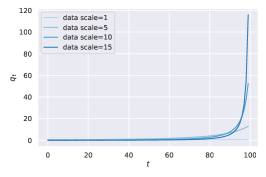
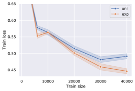
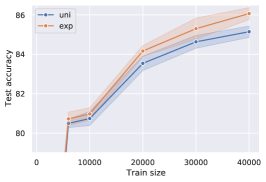
Figure 1. Comparison of dynamic schedule and uniform schedule on different data scale. Left pane is the influence by iteration estimated by retraining. The rest two panes are performance of DNN trained on the MNIST35 dataset with a varying total number of training samples, when the exponential influence is estimated on a randomly-generated auxiliary dataset.

Comparison of dynamic schedule and uniform schedule on different data scale.

We first show the estimated influence of step noise $q_{t}$ (by retraining the private learning algorithms) in Fig. 1 Left. We see the trends of influence are approximately in an exponential form of $t$. By Eq. 10, the resultant schedule on noise scale $\sigma_{t}$ will be a normalized exponential decay. This observation motivates the use of exponential decay schedule in practice.

To estimate the influence without extra privacy costs, we use an auxiliary set, which is randomly sampled from Gaussian distribution, to pick the proper influence curvature parameterized by an exponential function. We use auxiliary synthesized datasets of the same size as the corresponding private datasets to tune the parameters. We vary the size of training data to examine the data efficiency of the dynamic schedule denoted as exp. For a fair comparison, we also choose the hyper-parameters of uniform schedule (uni) on the same auxiliary dataset. We show that as the training size increases, exp outperforms uni both on the training loss and the test accuracy. The result verifies our theoretic conclusion: dynamic schedule is more data efficient than the static schedule.

6. Conclusion

When a privacy budget is provided for a certain learning task, one has to carefully schedule the privacy usage through the learning process. Uniformly scheduling the budget has been widely used in literature whereas increasing evidence suggests that dynamically schedules could empirically outperform the uniform one. This paper provided a principled analysis on the problem of optimal budget allocation and connected the advantages of dynamic schedules to both the loss structure and the learning behavior. We further validated our results through empirical studies.

Appendix A Social Impact

The wide usage of personal data in training machine learning has led to huge successes in many application domains but is also accompanied by rising concerns on privacy protection due to the sensitive information in the data. The development of privacy-preserving algorithms has become one of critical research areas of machine learning, in which the key challenge is to train high performance models under the constraint of a given privacy budget, or how much sensitive information can be accessed during the training phase. Differential privacy provided a principled framework to quantify the privacy budget, under which researchers proposed various schemes to schedule the budget usage during a learning process, yet there is a lack of systematical studies on when and why some schedules are better than other. Our efforts in this paper are among the first to study and compare the effectiveness of these schedules from a rigorous optimization perspective. Our theoretical results can benefit any privacy-preserving machine learning practitioners to efficiently and effectively choose proper privacy schedules tailored to their learning tasks.

Appendix B Comparison of algorithms

Here we elaborate the meaning of algorithm names in Table 1. Asymptotic upper bounds are achieved when sample size $N$ approaches infinity. Both $R$ and $R_{\epsilon,\delta}$ with $R_{\epsilon,\delta}<R$ are the privacy budgets of corresponding algorithms. Specifically, $R_{\epsilon,\delta}=\epsilon^{2}/\ln(1/\delta)<R$ when the private algorithm is $(\epsilon,\delta)$-DP with $\epsilon\leq 2\ln(1/\delta)$.

PGD+Adv. Adv denotes the Advanced Composition method (Bassily et al., 2014). The method assumes that loss function is $1$-strongly convex which implies the PL condition and optimized variable is in a convex set of diameter $1$ w.r.t. $l_{2}$ norm.

PGD+MA and the adjusted-utility version. MA denotes the Moment Accountant (Abadi et al., 2016) which improve the composed privacy bound versus the Advanced Composition. The improvement on privacy bound lead to a enhanced utility bound, as a result.

PGD+Adv+BBImp. The dynamic method assumes that the loss is $1$-strongly convex and data comes in stream with $n\leq N$ samples at each round. Their utility upper bound is achieved at some probability $p$ with any positive $c$.

Adam+MA. The authors prove a convergence bound for the gradient norms which is extended to loss bound by using PL condition. They also presents the results for AdaGrad and GD which are basically of the same upper bound. Out theorems improve their bound by using the recursive derivation based on the PL condition, while their bound is a simple application of the condition on the gradient norm bound.

GD, Non-Private. This method does not inject noise into gradients but limit the number of iterations. With the bound, we can see that our utility bound are optimal with dynamic schedule.

GD+zCDP. We discussed the static and dynamic schedule for the gradient descent method where the dynamic noise influence is the key to tighten the bound.

Momentum+zCDP. Different from the GD+zCDP, momentum methods will have two phase of utility upper bound. When $T$ is small than some positive constant $\hat{T}$, the bound is as tight as the non-private one. Afterwards, the momentum has a bound degraded as the GD bound.

Appendix C Preliminaries

C.1. Privacy

Lemma C.1 (Composition & Post-processing).

Let two mechanisms be $M:\mathcal{D}^{n}\rightarrow{\mathcal{Y}}$ and $M^{\prime}:{\mathcal{D}}^{n}\times{\mathcal{Y}}\rightarrow{\mathcal{Z}}$. Suppose $M$ satisfies $(\rho_{1},a)$-zCDP and $M^{\prime}(\cdot,y)$ satisfies $(\rho_{2},a)$-zCDP for $\forall y\in{\mathcal{Y}}$. Then, mechanism $M^{\prime\prime}:{\mathcal{D}}^{n}\rightarrow{\mathcal{Z}}$ (defined by $M^{\prime\prime}(x)=M^{\prime}(x,M(x))$) satisfies $(\rho_{1}+\rho_{2})$-zCDP.

Definition C.0 (Sensitivity).

The sensitivity of a gradient query $\nabla_{t}$ to the dataset $\{x_{i}\}_{i=1}^{N}$ is

$$\Delta_{2}(\nabla_{t}) =\max_{n}\left\|{1\over N}\sum\nolimits_{j=1,j\neq n}^{N}\nabla_{t}^{(j)}-{1\over N}\sum\nolimits_{j=1}^{N}\nabla_{t}^{(j)}\right\|_{2}$$

(18) $$={1\over N}\max_{n}\left\|\nabla^{(n)}_{t}\right\|_{2}$$

where $\nabla^{(n)}_{t}$ denotes the gradient of the $n$-th sample.

Lemma C.3 (Gaussian mechanism (Bun and Steinke, 2016)).

Let $f:{\mathcal{D}}^{n}\rightarrow{\mathcal{Z}}$ have sensitivity $\Delta$. Define a randomized algorithm $M:{\mathcal{D}}^{n}\rightarrow{\mathcal{Z}}$ by $M(x)\leftarrow f(x)+{\mathcal{N}}(0,\Delta^{2}\sigma^{2}I)$. Then $M$ satisfies ${1\over 2\sigma^{2}}$-zCDP.

Lemma C.4 ((Bun and Steinke, 2016)).

If $M$ is a mechanism satisfying $\rho$-zCDP, then $M$ is $(\rho+2\sqrt{\rho\ln(1/\delta)},\delta)$-DP for any $\delta>0$.

By solving $\rho+2\sqrt{\rho\ln(1/\delta)}=\epsilon$, we can get $\rho=\epsilon+2\ln(1/\delta)+2\sqrt{\ln(1/\delta)(\epsilon+\ln(1/\delta)}$.

C.2. Auxiliary lemmas

Lemma C.5.

If $\max_{n}\left\|x_{n}\right\|_{2}=1$ and ${1\over N}\sum_{n}x_{n}=0$, then the gradient sensitivity of the squared loss will be

$$\Delta_{2}(\nabla)=\max_{i}{1\over N}\sqrt{2f(\theta;x_{i})}\left\|x_{i}\right\|_{2}\leq{1\over 2}(DM\left\|\theta\right\|^{2}+1),$$

where $\Theta_{{\mathcal{M}}}$ is the set of all possible parameters $\theta_{t}$ generated by the learning algorithm ${\mathcal{M}}$.

Proof.

According to the definition of sensitivity in Eq. 18, we have

$$\Delta_{2}(\nabla)=\max_{i}\left\|\nabla^{(i)}\right\|_{2}=\max_{n}{1\over n}\left\|A^{(i)}\theta-x_{i}\right\|_{2}$$

where we use $i$ denotes the index of sample in the dataset. Here, we assume it is constant 1. We may get

$$\left\|A^{(i)}\theta-x_{i}\right\|_{2}^{2} =\left\|x_{i}(x_{i}^{\top}\theta-1)\right\|_{2}^{2}$$

(19) $$=(x_{i}^{\top}\theta-1)^{2}\left\|x_{i}\right\|_{2}^{2}=2f(\theta;x_{i})\left\|x_{i}\right\|_{2}^{2}$$

where $f(\theta;x_{i})={1\over 2}(x_{i}^{\top}\theta-1)^{2}$. Thus,

$$\Delta_{2}(\nabla)=\max_{i}{1\over N}\sqrt{2f(\theta;x_{i})}\left\|x_{i}\right\|_{2}$$

Since $\left\|x_{n}\right\|_{2}\leq 1$ and ${1\over N}\sum_{n=1}^{N}x_{n}=0$,

$$f(\theta) ={1\over 2N}\sum_{n=1}^{N}[(x_{n}^{\top}\theta)^{2}-2x_{n}^{\top}\theta+1]$$

$$\leq{1\over 2N}\sum_{n=1}^{N}[(\left\|x_{n}\right\|\left\|\theta\right\|)^{2}+1]$$

$$\leq{1\over 2}(DM\left\|\theta\right\|^{2}+1)$$

∎

Lemma C.6.

Assume assumptions in Theorem 4.6 are satisfied. Given variables defined in Theorem 4.6, the following inequality holds true:

$$\sum_{t=1}^{T}\gamma^{T-t}{2(1-\beta)\eta_{t}\over b_{t}}\sum\nolimits_{i=1}^{t}\beta^{t-i}\left\|\nabla_{t}-\nabla_{i}\right\|^{2}$$

$$\leq{\eta^{3}_{0}\beta\gamma\over 2M(1-\beta)^{3}(\gamma-\beta)^{2}}\sum_{i=1}^{T-1}\gamma^{T-i}\left\|v_{i+1}\right\|^{2}.$$

Proof.

We first handle the inner summation. By smoothness, the inequality $\left\|\nabla f(x)-\nabla f(y)\right\|\leq M\left\|x-y\right\|$ holds true. Thus,

$$\quad\sum\nolimits_{i=1}^{t}\beta^{t-i}\left\|\nabla_{t}-\nabla_{i}\right\|^{2}$$

$$\leq M^{2}\sum\nolimits_{i=1}^{t}\beta^{t-i}\left\|\theta_{t}-\theta_{i}\right\|^{2}$$

$$=M^{2}\sum\nolimits_{k=0}^{t-1}\beta^{k}\left\|\theta_{t}-\theta_{t-k}\right\|^{2}$$

$$=M^{2}\sum\nolimits_{k=0}^{t-1}\beta^{k}\left\|\sum\nolimits_{i=t-k}^{t-1}\eta_{i}v_{i+1}/b_{i}\right\|^{2}$$

$$\leq M^{2}\sum\nolimits_{k=0}^{t-1}\beta^{k}\left(\sum\nolimits_{j=t-k}^{t-1}\eta_{j}^{2}/b_{j}^{2}\right)\left(\sum\nolimits_{i=t-k}^{t-1}\left\|v_{i+1}\right\|^{2}\right)$$

where the last inequality is by Cauchy-Schwartz inequality. Because ${1\over b_{t}}={1\over 1-\beta^{t}}\leq{1\over 1-\beta}$ and $\eta_{t}={\eta_{0}\over 2M}$,

(20) $$\quad\sum\nolimits_{i=1}^{t}\beta^{t-i}\left\|\nabla_{t}-\nabla_{i}\right\|^{2}$$

$$\leq{\eta^{2}_{0}\over 4(1-\beta)^{2}}\sum\nolimits_{k=0}^{t-1}\beta^{k}k\sum\nolimits_{i=t-k}^{t-1}\left\|v_{i+1}\right\|^{2}$$

$$={\eta^{2}_{0}\over 4(1-\beta)^{2}}\sum\nolimits_{k=0}^{t-1}\beta^{k}k\sum\nolimits_{i=1}^{t-1}\left\|v_{i+1}\right\|^{2}\mathbb{I}(i\geq t-k)$$

$$={\eta^{2}_{0}\over 4(1-\beta)^{2}}\sum\nolimits_{i=1}^{t-1}\left\|v_{i+1}\right\|^{2}\sum\nolimits_{k=0}^{t-1}\beta^{k}k\mathbb{I}(k\geq t-i)$$

(21) $$={\eta^{2}_{0}\over 4(1-\beta)^{2}}\sum\nolimits_{i=1}^{t-1}\left\|v_{i+1}\right\|^{2}\sum\nolimits_{k=t-i}^{t-1}\beta^{k}k$$

where $\mathbb{I}(\cdot)$ is the indicating function which output $1$ if the condition holds true, otherwise $0$.

Denote the left-hand-side of the conclusion as LHS. We plug Eq. 21 into LHS to get

$$\operatorname{LHS} \leq\sum_{t=1}^{T}\gamma^{T-t}{1\over b_{t}}{\eta^{3}_{0}\over 4M(1-\beta)}\sum\nolimits_{i=1}^{t-1}\left\|v_{i+1}\right\|^{2}\sum\nolimits_{k=t-i}^{t-1}\beta^{k}k$$

$$\leq{\eta^{3}_{0}\over 4M(1-\beta)^{2}}\sum_{t=1}^{T}\gamma^{T-t}\sum\nolimits_{i=1}^{t-1}\left\|v_{i+1}\right\|^{2}\sum\nolimits_{k=t-i}^{t-1}\beta^{k}k$$

where we relax the upper bound by ${1\over b_{t}}={1\over 1-\beta^{t}}\leq{1\over 1-\beta}$. Using Lemma C.7 can directly lead to the conclusion:

$$\operatorname{LHS} \leq{\eta^{3}_{0}\beta\gamma\over 2M(1-\beta)^{3}(\gamma-\beta)^{2}}\sum_{i=1}^{T-1}\gamma^{T-i}\left\|v_{i+1}\right\|^{2}.$$

∎

Lemma C.7.

Given variables defined in Theorem 4.6, the following inequality holds true:

$$\sum_{t=1}^{T}\gamma^{T-t}\sum\nolimits_{i=1}^{t-1}\left\|v_{i+1}\right\|^{2}\sum\nolimits_{k=t-i}^{t-1}k\beta^{k}$$

$$\leq{2\beta\gamma\over(\gamma-\beta)^{2}(1-\beta)}\sum_{i=1}^{T-1}\gamma^{T-i}\left\|v_{i+1}\right\|^{2}.$$

Proof.

We first derive the summation:

$$\quad U_{1}(t,i)\triangleq\sum\nolimits_{k=t-i}^{t-1}\beta^{k}k$$

$$=\sum\nolimits_{k=t-i}^{t-1}\sum\nolimits_{j=1}^{k}\beta^{k}$$

$$=\sum\nolimits_{k=t-i}^{t-1}\sum\nolimits_{j=1}^{t-1}\beta^{k}\mathbb{I}(j\leq k)$$

$$=\sum\nolimits_{j=1}^{t-1}\sum\nolimits_{k=\max(t-i,j)}^{t-1}\beta^{k}$$

$$=\sum\nolimits_{j=1}^{t-1}{\beta^{\max(t-i,j)}-\beta^{t}\over 1-\beta}$$

$$={1\over 1-\beta}\left((t-i)\beta^{t-i}+{\beta^{t-i+1}-\beta^{t}\over 1-\beta}-{\beta-\beta^{t}\over 1-\beta}\right)$$

$$={1\over 1-\beta}\left((t-i)\beta^{t-i}+{\beta^{t-i+1}-\beta\over 1-\beta}\right)$$

Now, we substitute $U_{1}(t,i)$ into LHS and replace $t-i$ by $j$, i.e., $t=j+i$, to get

$$\operatorname{LHS} =\sum_{t=1}^{T}\gamma^{T-t}\sum_{i=1}^{t-1}\left\|v_{i+1}\right\|^{2}{1\over 1-\beta}\left((t-i)\beta^{t-i}+{\beta^{t-i+1}-\beta\over 1-\beta}\right)$$

$$=\sum_{i=1}^{T-1}\left\|v_{i+1}\right\|^{2}\sum_{t=i+1}^{T}\gamma^{T-t}{1\over 1-\beta}\left((t-i)\beta^{t-i}+{\beta^{t-i+1}-\beta\over 1-\beta}\right)$$

$$=\sum_{i=1}^{T-1}\left\|v_{i+1}\right\|^{2}\sum_{j=1}^{T-i}\gamma^{T-(j+i)}{1\over 1-\beta}\left(j\beta^{j}+{\beta^{j+1}-\beta\over 1-\beta}\right)$$

$$=\sum_{i=1}^{T-1}\gamma^{T-i}\left\|v_{i+1}\right\|^{2}\sum_{j=1}^{T-i}\gamma^{-j}{1\over 1-\beta}\left(j\beta^{j}+{\beta^{j+1}-\beta\over 1-\beta}\right)$$

$$\leq{1\over 1-\beta}\sum_{i=1}^{T-1}\gamma^{T-i}\left\|v_{i+1}\right\|^{2}\sum_{j=1}^{T-i}\left(j\left({\beta\over\gamma}\right)^{j}+{\beta\over 1-\beta}\left({\beta\over\gamma}\right)^{j}\right)$$

Let $a=\beta/\gamma$, we show

$$\sum_{j=1}^{T-i}ja^{j} =\sum_{j=1}^{T-i}\sum_{o=1}^{j}a^{j}$$

$$=\sum_{o=1}^{T-i}\sum_{j=o}^{T-i}a^{j}$$

$$=\sum_{o=1}^{T-i}({a^{o}-a^{T-i+1}\over 1-a})$$

$$={a-a^{T-i+1}\over(1-a)^{2}}-(T-i){a^{T-i+1}\over 1-a}$$

$$\leq{a\over(1-a)^{2}}.$$

Thus,

$$\operatorname{LHS} \leq{1\over 1-\beta}\sum_{i=1}^{T-1}\gamma^{T-i}\left\|v_{i+1}\right\|^{2}\left({a\over(1-a)^{2}}+{\beta\over 1-\beta}\sum_{j=1}^{T-i}a^{j}\right)$$

$$\leq{1\over 1-\beta}\sum_{i=1}^{T-1}\gamma^{T-i}\left\|v_{i+1}\right\|^{2}\left({a\over(1-a)^{2}}+{\beta\over 1-\beta}{a\over 1-a}\right)$$

$$\leq{a\over(1-a)^{2}(1-\beta)}\sum_{i=1}^{T-1}\gamma^{T-i}\left\|v_{i+1}\right\|^{2}$$

Because $\gamma<1$, $\beta<a=\beta/\gamma$ and

$${a\over(1-a)^{2}}+{\beta\over 1-\beta}{a\over 1-a}\leq{2a\over(1-a)^{2}}.$$

Therefore,

$$\operatorname{LHS} \leq{2a\over(1-a)^{2}(1-\beta)}\sum_{i=1}^{T-1}\gamma^{T-i}\left\|v_{i+1}\right\|^{2}$$

$$={2\beta\gamma\over(\gamma-\beta)^{2}(1-\beta)}\sum_{i=1}^{T-1}\gamma^{T-i}\left\|v_{i+1}\right\|^{2}$$

∎

Lemma C.8.

Suppose $\gamma\in(0,1)$ and $\beta\in(0,1)$. Define

$$\hat{T}=\max t~{}{\text{s.t.}}~{}\gamma^{t-1}\geq{1-\beta\over 1-\beta^{t}}.$$

If $t\leq\hat{T}$, ${1-\beta\over 1-\beta^{t}}\leq\gamma^{t-1}$ for $t=1,\dots,T$. If $t>\hat{T}$, ${1-\beta\over 1-\beta^{t}}<\gamma^{\hat{T}-1}$.

Proof.

Define $h(t)=\gamma^{t-1}(1-\beta^{t})$ whose derivatives are

$$h^{\prime}(t) =\gamma^{t-1}(1-\beta^{t})\ln\gamma+\gamma^{t-1}(-\beta^{t})\ln\beta$$

$$=\gamma^{t-1}\left[\ln\gamma-\beta^{t}(\ln\gamma+\ln\beta)\right]$$

$$=\gamma^{t-1}\left[1-\beta^{t}(1+\log_{\gamma}\beta)\right]\ln\gamma.$$

Simple calculation shows $\left.1-\beta^{t}(1+\log_{\gamma}\beta)\right|_{t=0}=-\log_{\gamma}\beta<0$ and $\lim_{t\rightarrow+\infty}1-\beta^{t}(1+\log_{\gamma}\beta)=1$. When $t=-\log_{\beta}(1+\log_{\gamma}\beta)$ denoted as $t_{0}$, $1-\beta^{t}(1+\log_{\gamma}\beta)=0$. Because $1-\beta^{t}(1+\log_{\gamma}\beta)$ is monotonically increasing by $t$ and $\gamma^{t-1}\ln\gamma$ is negative, $h^{\prime}(t)\geq 0$ if $t\leq t_{0}$. Otherwise, $h^{\prime}(t)<0$. Therefore, $h(t)$ is a concave function. Because $h(1)=1-\beta$ and $h(\hat{T})=\gamma^{\hat{T}-1}(1-\beta^{\hat{T}})\geq 1-\beta>0$, $h(t)\geq 1-\beta$ for $t=1,\dots,\hat{T}$. Thus, for all $t\in[1,\hat{T}]$, we have ${1-\beta\over 1-\beta^{t}}\leq\gamma^{t-1}$.

For $t>\hat{T}$, because ${1-\beta\over 1-\beta^{t}}$ monotonically increases by $t$, we have ${1-\beta\over 1-\beta^{t}}<{1-\beta\over 1-\beta^{\hat{T}}}\leq\gamma^{\hat{T}-1}$. ∎

Appendix D Proofs

Proof of Theorem 3.5.

Because all sample gradient are $G$-Lipschitz continuous, the sensitivity of the averaged gradient is upper bounded by $G/N$. Based on Lemma C.3, the privacy cost of $g_{t}$ is $1\over 2\sigma_{t}^{2}$.

Here, we make the output of each iteration a tuple of $(\theta_{t+1},v_{t=1})$. For the $1$st iteration, because $\theta_{1}$ does not embrace private information by random initialization, the mapping,

$$\left[\begin{array}[]{cc}v_{2}\\ \theta_{2}\end{array}\right]=\left[\begin{array}[]{cc}g_{1}\\ \theta_{1}-\eta_{1}g_{1}\end{array}\right],$$

is $\hat{\rho}_{1}$-zCDP where $\hat{\rho}_{1}={1\over 2\sigma_{t}^{2}}$.

Suppose the output of the $t$-th iteration, $(\theta_{t},v_{t})$, is $\hat{\rho}_{t}$-zCDP. At each iteration, we have the following mapping $(\theta_{t},v_{t})\rightarrow(\theta_{t+1},v_{t+1})$ defined as

$$\left[\begin{array}[]{cc}v_{t+1}\\ \theta_{t+1}\end{array}\right]=\left[\begin{array}[]{cc}\phi(v_{t},g_{t})\\ \theta_{t}-\eta_{t}\phi(v_{t},g_{t})\end{array}\right].$$

Thus, the output tuple $(\theta_{t+1},v_{t+1})$ is $(\hat{\rho}_{t}+{1\over 2\sigma_{t}^{2}})$-zCDP by Lemma C.1.

Thus, the recursion implies that $(\theta_{T+1},v_{T+1})$ has privacy cost as

$$\hat{\rho}_{T+1}=\hat{\rho}_{T}+{1\over 2\sigma_{T}^{2}}=\cdots=\sum_{t=1}^{T}{1\over 2\sigma_{t}^{2}}={1\over 2}\sum_{t=1}^{T}\rho_{t}\leq{1\over 2}(R-R_{T})\leq{1\over 2}R.$$

Let $\rho=\hat{\rho}_{T+1}$. Then we can get the conclusion.∎

D.1. Gradient Descents

Proof of Theorem 4.2.

With the definition of smoothness in Definition 3.3 and Eq. 1, we have

$$f(\theta_{t+1})-f(\theta_{t}) \leq-\eta_{t}\nabla_{t}^{\top}(\nabla_{t}+G\sigma_{t}\nu_{t}/N)+{1\over 2}M\eta_{t}^{2}\left\|\nabla_{t}+G\sigma_{t}\nu_{t}/N\right\|^{2}$$

$$=-\eta_{t}(1-{1\over 2}M\eta_{t})\left\|\nabla_{t}\right\|^{2}-(1-M\eta_{t})\eta_{t}\nabla_{t}^{\top}G\sigma_{t}\nu_{t}/N+{1\over 2}M\eta_{t}^{2}\left\|G\sigma_{t}\nu_{t}/N\right\|^{2}$$

$$\leq-2\mu\eta_{t}(1-{1\over 2}M\eta_{t})(f(\theta_{t})-f(\theta^{*}))-(1-M\eta_{t})\eta_{t}\nabla_{t}^{\top}G\sigma_{t}\nu_{t}/N$$

$$\quad+{1\over 2}M\eta_{t}^{2}\left\|G\sigma_{t}\nu_{t}/N\right\|^{2}.$$

where the last inequality is due to the Polyak-Lojasiewicz condition. Taking expectation on both sides, we can obtain

$$\mathbb{E}[f(\theta_{t+1})]-\mathbb{E}[f(\theta_{t})] \leq-2\mu\eta_{t}(1-{M\over 2}\eta_{t})(\mathbb{E}[f(\theta_{t})]-f(\theta^{*}))+{M\over 2}(\eta_{t}G\sigma_{t}/N)^{2}\mathbb{E}\left\|\nu_{t}\right\|^{2}$$

which can be reformulated by substacting $f(\theta^{*})$ on both sides and re-arranged as

$$\mathbb{E}[f(\theta_{t+1})]-f(\theta^{*}) \leq\left(1-2\mu\eta_{t}(1-{M\over 2}\eta_{t})\right)(\mathbb{E}[f(\theta_{t})]-f(\theta^{*}))+{M\over 2}(\eta_{t}G\sigma_{t}/N)^{2}D$$

Recursively using the inequality, we can get

$$\mathbb{E}[f(\theta_{T+1})]-f(\theta^{*}) \leq\prod_{t=1}^{T}\left(1-2\mu\eta_{t}(1-{M\over 2}\eta_{t})\right)(\mathbb{E}[f(\theta_{1})]-f(\theta^{*}))$$

$$\quad+{MD\over 2}\sum_{t=1}^{T}\prod_{i=t+1}^{T}\left(1-2\mu\eta_{i}(1-{M\over 2}\eta_{i})\right)(\eta_{t}G\sigma_{t}/N)^{2}.$$

Let $\eta_{t}\equiv 1/M$. Then the above inequality can be simplified as

$$\mathbb{E}[f(\theta_{T+1})]-f(\theta^{*}) \leq\gamma^{T}(\mathbb{E}[f(\theta_{1})]-f(\theta^{*}))+R\sum_{t=1}^{T}\gamma^{T-t}{MD\over 2R}\left({\eta_{t}G\over N}\right)^{2}\sigma_{t}^{2}$$

$$=\gamma^{T}(\mathbb{E}[f(\theta_{1})]-f(\theta^{*}))+R\sum_{t=1}^{T}\gamma^{T-t}\alpha\sigma_{t}^{2}(\mathbb{E}[f(\theta_{1})]-f(\theta^{*}))$$

$$=\left(\gamma^{T}+R\sum\nolimits_{t=1}^{T}q_{t}\sigma_{t}^{2}\right)(f(\theta_{1})-f(\theta^{*}))$$

∎

Proof of Theorem 4.3.

The minimizer of the upper bound of Eq. 7 can be written as

(22) $$T^{*} =\operatorname*{arg\,min}_{T}\gamma^{T}+\alpha\kappa(1-\gamma^{T})T$$

where we substitute $\sigma^{2}=T/R$ in the second line. To find the convex minimization problem, we need to vanishing its gradient which involves an equation like $T\gamma^{T}=c$ for some real constant $c$. However, the solution is $W_{k}(c)$ for some integer $k$ where $W$ is Lambert W function which does not have a simple analytical form. Instead, because $\gamma^{T}>0$, we can minimize a surrogate upper bound as following

(23) $$T^{*} =\operatorname*{arg\,min}_{T}\gamma^{T}+\alpha\kappa T={1\over\ln(1/\gamma)}\ln\left({\ln(1/\gamma)\over\kappa\alpha}\right),\text{ if }\kappa\alpha+\ln\gamma<0$$

where we use the surrogate upper bound in the second line and utilize $\gamma=1-{1\over\kappa}$. However, the minimizer of the surrogate objective is not optimal for the original objective. When $\kappa$ is large, the term, $-\alpha\kappa\gamma^{T}T$, cannot be neglected as we expect. On the other hands, $T$ suffers from explosion if $\kappa\rightarrow\infty$ and meanwhile $1/\gamma\rightarrow_{+}1$. The tendency is counterintuitive since a small $T$ should be taken for sharp losses. To fix the issue, we change the form of $T^{*}$ as

(24) $$T^{*}={1\over\ln(1/\gamma)}\ln\left(1+{\ln(1/\gamma)\over\alpha}\right),$$

which gradually converges to $0$ as $\kappa\rightarrow\infty$.

Now we substitute Eq. 24 into the original objective function, Eq. 22, to get

(25) $$\operatorname{ERUB}^{\text{uniform}} ={1\over 1+\ln(1/\gamma)/\alpha}\left[1+\kappa\ln\left(1+{\ln(1/\gamma)\over\alpha}\right)\right].$$

Notice that

$$\ln(1/\gamma) =\ln(\kappa/(\kappa-1))=\ln(1+1/(\kappa-1))\leq{1\over\kappa-1}\leq{1\over c\kappa}$$

because $\kappa\geq{1\over 1-c}>1$ for some constant $c\in(0,1)$. In addition,

$$\ln(1/\gamma) =-\ln(1-1/\kappa)\geq 1/\kappa.$$

Now, we can get the upper bound of Eq. 25 as

$$\operatorname{ERUB}^{\text{uniform}} \leq{\kappa\over\kappa+1/\alpha}\left[1+\kappa\ln\left(1+{1\over c\kappa\alpha}\right)\right]$$

$$\leq c_{1}{\kappa\over\kappa+1/\alpha}\kappa\left[\ln\left(1+{1\over\kappa\alpha}\right)+\ln({1\over c}))\right]$$

$$\leq c_{1}c_{2}{\kappa^{2}\over\kappa+1/\alpha}\ln\left(1+{1\over\kappa\alpha}\right)$$

for some constants $c_{1},c_{2}$ and large enough $1\over\alpha$. Also, we can get the lower bound

$$\operatorname{ERUB}^{\text{uniform}} \geq{c\kappa\over c\kappa+1/\alpha}\left[1+\kappa\ln\left(1+{1\over\kappa\alpha}\right)\right]\geq c{\kappa^{2}\over\kappa+1/\alpha}\ln\left(1+{1\over\kappa\alpha}\right).$$

where we use the condition $c\in(0,1)$. Thus, $\operatorname{ERUB}^{\text{uniform}}=\Theta\left({\kappa^{2}\over\kappa+1/\alpha}\ln\left(1+{1\over\kappa\alpha}\right)\right)$.∎

Proof of Lemma 4.4.

By $\sum_{t=1}^{T}\sigma^{-2}=R$ and Cauchy-Schwarz inequality, we can derive the achievable lower bound as

$$R\sum_{t}q_{t}\sigma_{t}^{2}=\sum_{t}{1\over\sigma_{t}^{2}}\sum_{t}q_{t}\sigma_{t}^{2}\geq\left(\sum_{t=1}^{T}\sqrt{q_{t}}\right)^{2}$$

where the inequality becomes equality if and only if ${s/\sigma_{t}^{2}}=q_{t}\sigma_{t}^{2}$, i.e., $\sigma_{t}=(s/q_{t})^{1/4}$, for some positive constant $s$. The equality $\sum_{t=1}^{T}\sigma_{t}^{-2}=R$ immediately suggests $\sqrt{s}={1\over R}\sum_{t=1}^{T}\sqrt{q_{t}}$. Thus, we get the $\sigma_{t}$.

Notice

(26) $$T\sum_{t=1}^{T}q_{t}-\left(\sum\nolimits_{t=1}^{T}\sqrt{q_{t}}\right)^{2}=T^{2}{1\over T}\sum_{t=1}^{T}\left(\sqrt{q_{t}}-{1\over T}\sum_{i=1}^{T}\sqrt{q_{i}}\right)^{2}=T^{2}\operatorname{Var}[q_{t}]$$

where the variance is w.r.t. $t$. ∎

Proof of Theorem 4.5.

The upper bound of Eq. 7 can be written as

$$\text{ERUB}^{\text{dyn}} =\gamma^{T}+\sum\nolimits_{t=1}^{T}\gamma^{T-t}\alpha R\sigma^{2}_{t}$$

$$=\gamma^{T}+\alpha\left(\sum\nolimits_{t=1}^{T}\sqrt{\gamma^{T-t}}\right)^{2}$$

$$=\gamma^{T}+\alpha\left({1-\gamma^{T/2}\over 1-\sqrt{\gamma}}\right)^{2}$$

where we make use of Lemma 4.4. Then, the minimizer of the ERUB is

$$T^{*} =\operatorname*{arg\,min}_{T}\gamma^{T}+\alpha\left({1-\gamma^{T/2}\over 1-\sqrt{\gamma}}\right)^{2}$$

(27) $$=2\log_{\gamma}\left({\alpha\over\alpha+(1-\sqrt{\gamma})^{2}}\right).$$

We can substitute Eq. 27 into $\text{ERUB}^{\text{dyn}}$ to get

$$\operatorname{ERUB}^{\text{dyn}}_{\min} =\left({\alpha\over\alpha+(1-\sqrt{\gamma})^{2}}\right)^{2}+\alpha\left({1\over 1-\sqrt{\gamma}}\right)^{2}\left(1-{\alpha\over\alpha+(1-\sqrt{\gamma})^{2}}\right)^{2}$$

$$=\left({\alpha(1-\sqrt{\gamma})^{-2}\over\alpha(1-\sqrt{\gamma})^{-2}+1}\right)^{2}+{\alpha(1-\sqrt{\gamma})^{-2}\over\left(\alpha(1-\sqrt{\gamma})^{-2}+1\right)^{2}}$$

$$={\alpha(1-\sqrt{\gamma})^{-2}\over\alpha(1-\sqrt{\gamma})^{-2}+1}$$

Notice that $\left(1-\sqrt{\gamma}\right)^{-2}=\kappa^{2}+\kappa^{2}-\kappa+2\kappa\sqrt{\kappa(\kappa-1)}=\kappa(2\kappa-1+2\sqrt{\kappa(\kappa-1)})$ and it is bounded by

$$\kappa(2\kappa-1+2\sqrt{\kappa(\kappa-1)})\leq 4\kappa^{2},$$

$$\kappa(2\kappa-1+2\sqrt{\kappa(\kappa-1)})\geq\kappa(2\kappa-(3\kappa-2)+2\sqrt{(\kappa-1)(\kappa-1)})=\kappa(-\kappa+2+2\kappa-2)=\kappa^{2}.$$

Therefore, $\kappa\leq\left(1-\sqrt{\gamma}\right)^{-1}\leq 2\kappa$, with which we can derive

$$\operatorname{ERUB}^{\text{dyn}}_{\min} \leq 4{\kappa^{2}\alpha\over\kappa^{2}\alpha+1},$$

$$\operatorname{ERUB}^{\text{dyn}}_{\min} \geq{\kappa^{2}\alpha\over 4\kappa^{2}\alpha+1}\geq{1\over 4}{\kappa^{2}\alpha\over\kappa^{2}\alpha+1}.$$

Thus, $\operatorname{ERUB}^{\text{dyn}}_{\min}=\Theta\left({\kappa^{2}\alpha\over\kappa^{2}\alpha+1}\right)$.∎

D.2. Gradient Descents with Momentum

Proof of Theorem 4.6.

Without loss of generality, we absorb the $C\sigma_{t}/N$ into the variance of $\nu_{t}$ such that $\nu_{t}\sim\mathcal{N}(0,{C\sigma_{t}^{2}\over N}I)$ and $g_{t}\leftarrow\nabla_{t}+\nu_{t}$. Define $b_{t}=1-\beta^{t}$.

By smoothness and Eq. 1, we have

$$f(\theta_{t+1})-f(\theta_{t}) \leq\nabla_{t}^{\top}(\theta_{t+1}-\theta_{t})+{1\over 2}M\left\|\theta_{t+1}-\theta_{t}\right\|^{2}$$

$$=-{\eta_{t}\over b_{t}^{2}}b_{t}\nabla_{t}^{\top}v_{t+1}+{1\over 2}M{\eta_{t}^{2}\over b_{t}^{2}}\left\|v_{t+1}\right\|^{2}$$

$$={\eta_{t}\over b_{t}^{2}}\left(\left\|b_{t}\nabla_{t}-v_{t+1}\right\|^{2}-\left\|b_{t}\nabla_{t}\right\|^{2}-\left\|v_{t+1}\right\|^{2}\right)+{1\over 2}M{\eta_{t}^{2}\over b_{t}^{2}}\left\|v_{t+1}\right\|^{2}$$

(28) $$={\eta_{t}\over b_{t}^{2}}\underbrace{\left\|b_{t}\nabla_{t}-v_{t+1}\right\|^{2}}_{U_{1}(t)}-\eta_{t}\left\|\nabla_{t}\right\|^{2}-{\eta_{t}\over b_{t}^{2}}(1-{1\over 2}M\eta_{t})\left\|v_{t+1}\right\|^{2},$$

where only the $U_{1}(t)$ is non-negative. Specifically, $U_{1}(t)$ describes the difference between current gradient and the average. We can expand $v_{t+1}$ to get an upper bound:

$$U_{1}(t) =\left\|b_{t}\nabla_{t}-v_{t+1}\right\|^{2}$$

$$=\left\|(1-\beta)\sum\nolimits_{i=1}^{t}\beta^{t-i}\nabla_{t}-(1-\beta)\sum\nolimits_{i=1}^{t}\beta^{t-i}g_{i}\right\|^{2}$$

$$=(1-\beta)^{2}\left\|\sum\nolimits_{i=1}^{t}\beta^{t-i}(\nabla_{t}-g_{i})\right\|^{2}$$

$$=(1-\beta)^{2}\left\|\sum\nolimits_{i=1}^{t}\beta^{t-i}(\nabla_{t}-\nabla_{i})+\sum\nolimits_{i=1}^{t}\beta^{t-i}(\nabla_{i}-g_{i})\right\|^{2}$$

$$\leq 2(1-\beta)^{2}\left[\left\|\sum\nolimits_{i=1}^{t}\beta^{t-i}(\nabla_{t}-\nabla_{i})\right\|^{2}+\left\|\sum\nolimits_{i=1}^{t}\beta^{t-i}(\nabla_{i}-g_{i})\right\|^{2}\right]$$

$$\leq 2(1-\beta)\left[b_{t}\underbrace{\sum\nolimits_{i=1}^{t}\beta^{t-i}\left\|\nabla_{t}-\nabla_{i}\right\|^{2}}_{U_{2}(t)\text{ (gradient variance)}}+(1-\beta)\underbrace{\left\|\sum\nolimits_{i=1}^{t}\beta^{t-i}\nu_{i}\right\|^{2}}_{\text{noise variance}}\right]$$

where we use $\left\|x+y\right\|^{2}\leq(\left\|x\right\|+\left\|y\right\|)^{2}\leq 2(\left\|x\right\|^{2}+\left\|y\right\|^{2})$. The last inequality can be proved by Cauchy-Schwartz inequality for each coordinate.

We plug the $U_{1}(t)$ into Eq. 28 and use the PL condition to get

$$f(\theta_{t+1})-f(\theta_{t}) \leq{\eta_{t}\over b_{t}^{2}}U_{1}(t)-\eta_{t}\left\|\nabla_{t}\right\|^{2}-{\eta_{t}\over b_{t}^{2}}(1-{1\over 2}M\eta_{t})\left\|v_{t+1}\right\|^{2}$$

$$\leq-\eta_{t}\left\|\nabla_{t}\right\|^{2}+{\eta_{t}\over b_{t}^{2}}2(1-\beta)\left[b_{t}U_{2}(t)+(1-\beta)\left\|\sum\nolimits_{i=1}^{t}\beta^{t-i}\nu_{i}\right\|^{2}\right]$$

$$\quad-{\eta_{t}\over b_{t}^{2}}(1-{1\over 2}M\eta_{t})\left\|v_{t+1}\right\|^{2}$$

$$\leq-2\mu\eta_{t}(f(\theta_{t})-f(\theta^{*}))+{2(1-\beta)\eta_{t}\over b_{t}}U_{2}(t)+{2(1-\beta)^{2}\eta_{t}\over b_{t}^{2}}\left\|\sum\nolimits_{i=1}^{t}\beta^{t-i}\nu_{i}\right\|^{2}$$

$$\quad-{\eta_{t}\over b_{t}^{2}}(1-{1\over 2}M\eta_{t})\left\|v_{t+1}\right\|^{2}.$$

Rearranging terms and taking expectation to show

$$\mathbb{E}[f(\theta_{t+1})]-f(\theta^{*}) \leq\gamma(\mathbb{E}[f(\theta_{t})]-f(\theta^{*}))+{2(1-\beta)^{2}\eta_{t}\over b_{t}^{2}}\sum\nolimits_{i=1}^{t}\beta^{t-i}\mathbb{E}\left\|\nu_{i}\right\|^{2}$$

$$\quad+{2(1-\beta)\eta_{t}\over b_{t}}\mathbb{E}[U_{2}(t)]-{\eta_{t}\over b_{t}^{2}}(1-{1\over 2}M\eta_{t})\mathbb{E}\left\|v_{t+1}\right\|^{2}$$

$$=\gamma(\mathbb{E}[f(\theta_{t})]-f(\theta^{*}))+{2(1-\beta)^{2}\eta_{t}\over b_{t}^{2}}\sum\nolimits_{i=1}^{t}\beta^{2(t-i)}{C^{2}D\sigma_{t}^{2}\over N^{2}}$$

$$\quad+{2(1-\beta)\eta_{t}\over b_{t}}\mathbb{E}[U_{2}(t)]-{\eta_{t}\over b_{t}^{2}}(1-{1\over 2}M\eta_{t})\mathbb{E}\left\|v_{t+1}\right\|^{2}$$

where $\gamma=1-\eta_{0}/\kappa=1-2\mu\eta_{t}$. The recursive inequality implies

$$\mathbb{E}[f(\theta_{T+1})]-f(\theta^{*}) \leq\gamma^{T}(f(\theta_{1})-f(\theta^{*}))+\sum_{t=1}^{T}\gamma^{T-t}{2(1-\beta)^{2}\eta_{t}\over b_{t}^{2}}\sum\nolimits_{i=1}^{t}\beta^{2(t-i)}{C^{2}D\sigma_{t}^{2}\over N^{2}}$$

$$\quad+\sum_{t=1}^{T}\gamma^{T-t}{2(1-\beta)\eta_{t}\over b_{t}}\mathbb{E}[U_{2}(t)]-\sum_{t=1}^{T}\gamma^{T-t}{\eta_{t}\over b_{t}^{2}}(1-{1\over 2}M\eta_{t})\mathbb{E}\left\|v_{t+1}\right\|^{2}$$

$$=\bigg{(}\gamma^{T}+2\eta_{0}\alpha R\underbrace{\sum\nolimits_{t=1}^{T}\gamma^{T-t}{(1-\beta)^{2}\over b_{t}^{2}}\sum\nolimits_{i=1}^{t}\beta^{2(t-i)}\sigma_{t}^{2}}_{U_{3}}\bigg{)}(f(\theta_{1})-f(\theta^{*}))$$

$$\quad+\underbrace{\sum_{t=1}^{T}\gamma^{T-t}{2(1-\beta)\eta_{t}\over b_{t}}\mathbb{E}[U_{2}(t)]-\sum_{t=1}^{T}\gamma^{T-t}{\eta_{t}\over b_{t}^{2}}(1-{1\over 2}M\eta_{t})\mathbb{E}\left\|v_{t+1}\right\|^{2}}_{U_{4}(t)}.$$

where we utilize $\alpha={DC^{2}\over 2MN^{2}R}{1\over f(\theta_{1})-f(\theta^{*})}$ and $\eta_{t}={\eta_{0}\over 2M}$.

By Lemma C.6, we have

$$\sum_{t=1}^{T}\gamma^{T-t}{2(1-\beta)\eta_{t}\over b_{t}}U_{2}(t) \leq{\eta^{3}_{0}\beta\gamma\over 2M(1-\beta)^{3}(\gamma-\beta)^{2}}\sum_{i=1}^{T-1}\gamma^{T-i}\left\|v_{i+1}\right\|^{2}.$$

Thus, by ${1\over b_{t}}\geq 1$,

$$U_{4}(t) \leq{\eta^{3}_{0}\beta\gamma\over 2M(1-\beta)^{3}(\gamma-\beta)^{2}}\sum_{i=1}^{T-1}\gamma^{T-i}\mathbb{E}\left\|v_{i+1}\right\|^{2}-{\eta_{0}\over 2M}(1-{\eta_{0}\over 4})\sum_{t=1}^{T}\gamma^{T-t}\mathbb{E}\left\|v_{t+1}\right\|^{2}$$

$$=-{\eta_{0}\over 2M}\zeta\sum_{t=1}^{T}\gamma^{T-t}\mathbb{E}\left\|v_{t+1}\right\|^{2}$$

where

$$\zeta=1-{1\over 4}\eta_{0}-{\beta\gamma\over(\gamma-\beta)^{2}(1-\beta)^{3}}\eta^{2}_{0}=1-{1\over 4}\eta_{0}-{\beta/\gamma\over(1-\beta/\gamma)^{2}(1-\beta)^{3}}\eta^{2}_{0}$$

When a small enough $\eta_{0}$, e.g., Specifically,

$$\eta_{0} \leq{(\gamma-\beta)^{2}(1-\beta)^{3}\over 8\beta\gamma}\left[\sqrt{1+{64\beta\gamma\over(\gamma-\beta)^{2}(1-\beta)^{3}}}-1\right]$$

$$={8\over\sqrt{1+{64\beta\gamma(\gamma-\beta)^{-2}(1-\beta)^{-3}}}+1}$$

We can have $\zeta\geq 0$.

By the definition of $U_{3}(T,\sigma)$, we can get

$$\mathbb{E}[f(\theta_{T+1})]-f(\theta^{*}) \leq\left(\gamma^{T}+2\eta_{0}\alpha RU_{3}(T,\sigma)\right)(f(\theta_{1})-f(\theta^{*}))-{\eta_{0}\over 2M}\zeta\sum_{t=1}^{T}\gamma^{T-t}\mathbb{E}\left\|v_{t+1}\right\|^{2}.$$

∎

Proof of Theorem 4.7.

Since $\sigma_{t}$ is static, by definition of $U_{3}$ in Theorem 4.6,

$$U_{3} =\sum\nolimits_{t=1}^{T}\gamma^{T-t}{(1-\beta)^{2}\over(1-\beta^{t})^{2}}\sum\nolimits_{i=1}^{t}\beta^{2(t-i)}\sigma^{2}$$

$$=\sigma^{2}\sum\nolimits_{t=1}^{T}\gamma^{T-t}{(1-\beta)^{2}\over(1-\beta^{t})^{2}}\sum\nolimits_{i=1}^{t}\beta^{2(t-i)}$$

$$=\sigma^{2}\sum\nolimits_{t=1}^{T}\gamma^{T-t}{(1-\beta)^{2}\over(1-\beta^{t})^{2}}{1-\beta^{2t}\over 1-\beta^{2}}$$

$$=\sigma^{2}\sum\nolimits_{t=1}^{T}\gamma^{T-t}{1-\beta\over 1-\beta^{t}}{1+\beta^{t}\over 1+\beta}.$$

Because ${1-\beta\over 1-\beta^{t}}{1+\beta^{t}\over 1+\beta}\leq 1$, the $U_{3}$ will be smaller than the corresponding summation in GD with uniform schedule.

By Lemma C.8, when $T>\hat{T}$, we can rewrite $U_{3}$ as

$$U_{3} \leq\sigma^{2}\sum\nolimits_{t=1}^{T}\gamma^{T-t}{1-\beta\over 1-\beta^{t}}$$

$$=\sigma^{2}\sum\nolimits_{t=1}^{\hat{T}}\gamma^{T-t}{1-\beta\over 1-\beta^{t}}+\sigma^{2}\sum\nolimits_{t=\hat{T}+1}^{T}\gamma^{T-t}{1-\beta\over 1-\beta^{t}}$$

$$\leq\sigma^{2}\sum\nolimits_{t=1}^{\hat{T}}\gamma^{T-t}\gamma^{t-1}+\sigma^{2}\sum\nolimits_{t=\hat{T}+1}^{T}\gamma^{T-t}\gamma^{\hat{T}-1}$$

$$=\sigma^{2}\gamma^{T-1}\hat{T}+\sigma^{2}\gamma^{\hat{T}-1}\sum\nolimits_{t=1}^{T-\hat{T}}\gamma^{T-\hat{T}-t}$$

$$=\sigma^{2}\gamma^{T-1}\hat{T}+\sigma^{2}{\gamma^{\hat{T}-1}-\gamma^{T-1}\over 1-\gamma}$$

$$={T\over\gamma R}\gamma^{T}\left(\hat{T}+{\gamma^{\hat{T}-T}-1\over 1-\gamma}\right)$$

where we use $\sigma^{2}=T/R$ in the last line. Without assuming $T>\hat{T}$, we can generally write the upper bound as

$$U_{3} \leq{T\over\gamma R}\gamma^{T}\left(\min\{\hat{T},T\}+\max\{{\gamma^{\hat{T}-T}-1\over 1-\gamma},0\}\right).$$

By Theorem 4.6, because $\zeta\geq 0$, we have

$$\operatorname{ERUB} \leq\gamma^{T}+2R\eta_{0}\alpha U_{3}$$

$$=\gamma^{T}(1+\frac{\alpha^{\prime}}{\gamma}T\left(\min\{\hat{T},T\}+\max\{{\gamma^{\hat{T}-T}-1\over 1-\gamma},0\}\right))$$

where $\alpha^{\prime}=2\eta_{0}\alpha$.

First, we consider $T\leq\hat{T}$. Use $T={1\over\ln(1/\gamma)}\ln\left(1+{\eta_{0}\over\kappa\alpha}\right)=\left\lceil{\mathcal{O}}\left({\kappa\over\eta_{0}}\ln\left(1+{\eta_{0}\over\kappa\alpha}\right)\right)\right\rceil$ to get

$$\operatorname{ERUB} \leq\left({\alpha\over\alpha+\eta_{0}/\kappa}\right)\left(1+\alpha^{\prime}\gamma^{-1}({2\over\ln(1/\gamma)}\ln\left(1+{\eta_{0}\over\kappa\alpha}\right))^{2}\right)$$

$$\leq\left({\alpha\over\alpha+\eta_{0}/\kappa}\right)\left(1+{8\kappa^{2}\alpha\over\eta_{0}\gamma}\ln^{2}\left(1+{\eta_{0}\over\kappa\alpha}\right)\right)$$

$$\leq{\mathcal{O}}\left({\kappa\over\kappa+\eta_{0}/\alpha}\left(1+{8\kappa^{2}\alpha\over\eta_{0}\gamma}\ln^{2}\left(1+{\eta_{0}\over\kappa\alpha}\right)\right)\right)$$

$$={\mathcal{O}}\left({\kappa\over\kappa+\eta_{0}/\alpha}\left(1+{4\kappa\over\gamma}\right)\right)$$

$$={\mathcal{O}}\left({\kappa^{2}\over\kappa+\eta_{0}/\alpha}\right)$$

where we used $\ln(1/\gamma)\geq\eta_{0}/\kappa$ and $\ln(1+x)\leq\sqrt{x}$ for any $x>0$.

Second, when $T>\hat{T}$,

$$\operatorname{ERUB} \leq\gamma^{T}(1+\frac{\alpha^{\prime}}{\gamma}T\left(\hat{T}+{\gamma^{\hat{T}-T}-1\over 1-\gamma}\right))$$

$$\leq{\mathcal{O}}\left(\gamma^{T}+\frac{2\alpha^{\prime}}{\gamma}T\kappa(\gamma^{\hat{T}}-\gamma^{T})\right).$$

Make use of $T=\left\lceil{1\over\ln(1/\gamma)}\ln\left(1+{\eta_{0}\over\kappa\alpha}\right)\right\rceil$ to show

$$\operatorname{ERUB} \leq{\mathcal{O}}\left({\kappa\over\kappa+\eta_{0}/\alpha}+\frac{4\kappa^{2}\alpha}{\eta_{0}\gamma}(\gamma^{\hat{T}}-{\kappa\over\kappa+\eta_{0}/\alpha})\ln\left(1+{\eta_{0}\over\kappa\alpha}\right)\right)$$

$$\leq{\mathcal{O}}\left({\kappa^{2}\over\kappa+\eta_{0}/\alpha}\gamma^{\hat{T}-1}\ln\left(1+{\eta_{0}\over\kappa\alpha}\right)\right).$$

∎

Proof of Theorem 4.8.

By Lemma C.8, we can rewrite $U_{3}$ as

$$U_{3} =\sum\nolimits_{t=1}^{T}\gamma^{T-t}{(1-\beta)^{2}\over(1-\beta^{t})^{2}}\sum\nolimits_{i=1}^{t}\beta^{2(t-i)}\sigma_{i}^{2}$$

$$\leq\sum\nolimits_{t=1}^{\hat{T}}\gamma^{T-t}\gamma^{2(t-1)}\sum\nolimits_{i=1}^{t}\beta^{2(t-i)}\sigma_{i}^{2}+\sum\nolimits_{t=\hat{T}+1}^{T}\gamma^{T-t}\gamma^{2(\hat{T}-1)}\sum\nolimits_{i=1}^{t}\beta^{2(t-i)}\sigma_{i}^{2}$$

$$\leq\gamma^{T-\hat{T}}\underbrace{\sum\nolimits_{t=1}^{\hat{T}}\gamma^{\hat{T}-t}\gamma^{2(t-1)}\sum\nolimits_{i=1}^{t}\beta^{2(t-i)}\sigma_{i}^{2}}_{V_{1}}+\gamma^{2(\hat{T}-1)}\underbrace{\sum\nolimits_{t=\hat{T}+1}^{T}\gamma^{T-t}\sum\nolimits_{i=1}^{t}\beta^{2(t-i)}\sigma_{i}^{2}}_{V_{2}}$$

We derive $V_{1}$ and $V_{2}$ separately.

For $V_{1}$, we can obtain the upper bound by

$$V_{1} =\sum\nolimits_{t=1}^{\hat{T}}\gamma^{\hat{T}-t}\gamma^{2(t-1)}\sum\nolimits_{i=1}^{t}\beta^{2(t-i)}\sigma_{i}^{2}$$

$$=\gamma^{\hat{T}-2}\sum\nolimits_{t=1}^{\hat{T}}\gamma^{t}\sum\nolimits_{i=1}^{t}\beta^{2(t-i)}\sigma_{i}^{2}$$

$$=\gamma^{\hat{T}-2}\sum\nolimits_{i=1}^{\hat{T}}\beta^{-2i}\sigma_{i}^{2}\sum\nolimits_{t=i}^{\hat{T}}\left(\gamma\beta^{2}\right)^{t}$$

$$=\gamma^{\hat{T}-2}\sum\nolimits_{i=1}^{\hat{T}}\beta^{-2i}\sigma_{i}^{2}{\left(\gamma\beta^{2}\right)^{i}-\left(\gamma\beta^{2}\right)^{\hat{T}+1}\over 1-\gamma\beta^{2}}$$

$$=\gamma^{2\hat{T}-3}\sum\nolimits_{i=1}^{\hat{T}}{\gamma^{i-\hat{T}-1}-\beta^{2(\hat{T}+1-i)}\over 1-\gamma\beta^{2}}\sigma_{i}^{2}$$

$$=\gamma^{2\hat{T}-3}\sum\nolimits_{i=1}^{\hat{T}}{1-(\gamma\beta^{2})^{\hat{T}+1-i}\over 1-\gamma\beta^{2}}\gamma^{i-\hat{T}-1}\sigma_{i}^{2}$$

$$\leq{\gamma^{\hat{T}}\over\gamma^{2}(1-\gamma\beta^{2})}\sum\nolimits_{i=1}^{\hat{T}}\gamma^{i}\sigma_{i}^{2}$$

$$\leq{\gamma^{\hat{T}}\over\gamma(\gamma-\beta^{2})}\sum\nolimits_{i=1}^{\hat{T}}\gamma^{i}\sigma_{i}^{2}$$

For $V_{2}$, we can derive

$$V_{2} =\sum\nolimits_{t=\hat{T}+1}^{T}\gamma^{T-t}\sum\nolimits_{i=1}^{t}\beta^{2(t-i)}\sigma_{i}^{2}$$

$$=\sum\nolimits_{t=1}^{T}\gamma^{T-t}\sum\nolimits_{i=1}^{t}\beta^{2(t-i)}\sigma_{i}^{2}-\sum\nolimits_{t=1}^{\hat{T}}\gamma^{T-t}\sum\nolimits_{i=1}^{t}\beta^{2(t-i)}\sigma_{i}^{2}$$

$$=\sum\nolimits_{t=1}^{T}\gamma^{T-t}\sum\nolimits_{i=1}^{t}\beta^{2(t-i)}\sigma_{i}^{2}-\gamma^{T-\hat{T}}\sum\nolimits_{t=1}^{\hat{T}}\gamma^{\hat{T}-t}\sum\nolimits_{i=1}^{t}\beta^{2(t-i)}\sigma_{i}^{2}.$$

We first consider the first term

$$\quad\sum\nolimits_{t=1}^{T}\gamma^{T-t}\sum\nolimits_{i=1}^{t}\beta^{2(t-i)}\sigma_{i}^{2}$$

$$=\sum\nolimits_{i=1}^{T}\sigma_{i}^{2}\sum\nolimits_{t=i}^{T}\gamma^{T-t}\beta^{2(t-i)}$$

$$=\sum\nolimits_{i=1}^{T}\gamma^{T}\beta^{-2i}\sigma_{i}^{2}\sum\nolimits_{t=i}^{T}\gamma^{-t}\beta^{2t}$$

$$=\sum\nolimits_{i=1}^{T}\gamma^{T}\beta^{-2i}\sigma_{i}^{2}{(\beta^{2}/\gamma)^{i}-(\beta^{2}/\gamma)^{T+1}\over 1-(\beta^{2}/\gamma)}$$

$$=\sum\nolimits_{i=1}^{T}{\gamma^{T+1-i}-\beta^{2(T+1-i)}\over\gamma-\beta^{2}}\sigma_{i}^{2}.$$

Similarly, we have

$$\quad\gamma^{T-\hat{T}}\sum\nolimits_{t=1}^{\hat{T}}\gamma^{\hat{T}-t}\sum\nolimits_{i=1}^{t}\beta^{2(t-i)}\sigma_{i}^{2}$$

$$=\gamma^{T-\hat{T}}\sum\nolimits_{i=1}^{\hat{T}}{\gamma^{\hat{T}+1-i}-\beta^{2(\hat{T}+1-i)}\over\gamma-\beta^{2}}\sigma_{i}^{2}$$

$$=\sum\nolimits_{i=1}^{\hat{T}}{\gamma^{T+1-i}-\gamma^{T-\hat{T}}\beta^{2(\hat{T}+1-i)}\over\gamma-\beta^{2}}\sigma_{i}^{2}.$$

Thus,

$$V_{2} =\sum\nolimits_{i=1}^{T}{\gamma^{T+1-i}-\beta^{2(T+1-i)}\over\gamma-\beta^{2}}\sigma_{i}^{2}-\sum\nolimits_{i=1}^{\hat{T}}{\gamma^{T+1-i}-\gamma^{T-\hat{T}}\beta^{2(\hat{T}+1-i)}\over\gamma-\beta^{2}}\sigma_{i}^{2}$$

$$=\sum\nolimits_{i=\hat{T}+1}^{T}{\gamma^{T+1-i}-\beta^{2(T+1-i)}\over\gamma-\beta^{2}}\sigma_{i}^{2}+\sum\nolimits_{i=1}^{\hat{T}}{\gamma^{T-\hat{T}}-\beta^{2(T-\hat{T})}\over\gamma-\beta^{2}}\beta^{2(\hat{T}+1-i)}\sigma_{i}^{2}$$

$$\leq\sum\nolimits_{i=\hat{T}+1}^{T}{\gamma^{T+1-i}-\beta^{2(T+1-i)}\over\gamma-\beta^{2}}\sigma_{i}^{2}+\sum\nolimits_{i=1}^{\hat{T}}{\gamma^{T-\hat{T}}\over\gamma-\beta^{2}}\beta^{2(\hat{T}+1-i)}\sigma_{i}^{2}.$$

Substitute $V_{1}$ and $V_{2}$ into $U_{3}$ to get

$$U_{3} \leq\gamma^{T}{1\over\gamma(\gamma-\beta^{2})}\sum\nolimits_{i=1}^{\hat{T}}\gamma^{i}\sigma_{i}^{2}+\gamma^{2\hat{T}-2}\sum\nolimits_{i=\hat{T}+1}^{T}{\gamma^{T+1-i}-\beta^{2(T+1-i)}\over\gamma-\beta^{2}}\sigma_{i}^{2}$$

$$\quad+\sum\nolimits_{i=1}^{\hat{T}}{\gamma^{T+\hat{T}-2}\over\gamma-\beta^{2}}\beta^{2(\hat{T}+1-i)}\sigma_{i}^{2}$$

$$\leq\left({\gamma^{T}\over\gamma(\gamma-\beta^{2})}\sum\nolimits_{i=1}^{\hat{T}}(\gamma^{i}+\gamma^{\hat{T}-1}\beta^{2(\hat{T}+1-i)})\sigma_{i}^{2}+\gamma^{2\hat{T}-2}\sum\nolimits_{i=\hat{T}+1}^{T}{\gamma^{T+1-i}-\beta^{2(T+1-i)}\over\gamma-\beta^{2}}\sigma_{i}^{2}\right)$$

$$\leq\left({2\gamma^{T}\over\gamma(\gamma-\beta^{2})}\sum\nolimits_{i=1}^{\hat{T}}\gamma^{i}\sigma_{i}^{2}+\gamma^{2\hat{T}-2}\sum\nolimits_{i=\hat{T}+1}^{T}{\gamma^{T+1-i}-\beta^{2(T+1-i)}\over\gamma-\beta^{2}}\sigma_{i}^{2}\right)$$

$$=\sum\nolimits_{t=1}^{T}q_{t}\sigma_{t}^{2}$$

where

$$q_{t} ={2\over\gamma(\gamma-\beta^{2})}\gamma^{T+t}\mathbb{I}_{T\leq\hat{T}}+\gamma^{2(\hat{T}-1)}{\gamma^{T+1-i}-\beta^{2(T+1-i)}\over\gamma-\beta^{2}}\gamma^{T-t}\mathbb{I}_{T>\hat{T}}$$

$$\leq c_{1}\gamma^{T+t}\mathbb{I}_{T\leq\hat{T}}+\gamma^{\hat{T}-1}c_{2}\gamma^{T-t}\mathbb{I}_{T>\hat{T}}$$

where $c_{1}={2\over\gamma(\gamma-\beta^{2})}$ and $c_{2}={\gamma^{2\hat{T}}\over\gamma-\beta^{2}}$.

When $T>\hat{T}$, by Lemma 4.4, the lower bound of $R\sum\nolimits_{t=1}^{T}q_{t}\sigma_{t}^{2}$ is

$$\left(\sum\nolimits_{t=1}^{T}\sqrt{q_{t}}\right)^{2} =\gamma^{T}\left(\sum\nolimits_{t=1}^{\hat{T}}\sqrt{c_{1}\gamma^{t}}+\sum\nolimits_{t=\hat{T}+1}^{T}\sqrt{\gamma^{\hat{T}-1}c_{2}\gamma^{-t}}\right)^{2}$$

$$=\gamma^{T}\left(\sqrt{c_{1}\gamma}\frac{1-\gamma^{\hat{T}/2}}{1-\sqrt{\gamma}}+\sqrt{c_{2}}\frac{1-\gamma^{(\hat{T}-T-1)/2}}{\sqrt{\gamma}-1}\right)^{2}$$

$$=\gamma^{T}\left(\sqrt{c_{1}\gamma}\frac{1-\gamma^{\hat{T}/2}}{1-\sqrt{\gamma}}+\sqrt{c_{2}}\frac{\gamma^{(\hat{T}-T-1)/2}-1}{1-\sqrt{\gamma}}\right)^{2}$$

$$\leq{\mathcal{O}}\left(c_{2}\left\{\frac{\gamma^{(\hat{T}-1)/2}-\gamma^{T/2}}{1-\sqrt{\gamma}}\right\}^{2}\right)$$

which is achieved when

$$\sigma_{t}^{2}={1\over R}\sum\nolimits_{i=1}^{T}\sqrt{q_{i}\over q_{t}}.$$

By Theorem 4.6, because $\zeta\geq 0$, we have

$$\operatorname{ERUB} \leq\gamma^{T}+2R\eta_{0}\alpha U_{3}$$

$$=\gamma^{T}+2\eta_{0}\alpha\sum\nolimits_{t=1}^{T}Rq_{t}\sigma_{t}^{2}.$$

And the minimum of the upper bound is

$$\operatorname{ERUB}_{\min} =\gamma^{T}+\alpha^{\prime}{\mathcal{O}}\left(\left\{\frac{\gamma^{(\hat{T}-1)/2}-\gamma^{T/2}}{1-\sqrt{\gamma}}\right\}^{2}\right)$$

where $\alpha^{\prime}={2\eta_{0}c_{2}\alpha}$. Let $T={2\over\ln(1/\gamma)}\ln\left(1+{\eta_{0}\over\kappa\alpha}\right)$. Then,

$$\operatorname{ERUB}_{\min} ={\mathcal{O}}\left(\left({\kappa\alpha\over\kappa\alpha+\eta_{0}}\right)^{2}+{\alpha^{\prime}\over(1-\sqrt{\gamma})^{2}}\left\{{{\gamma^{(\hat{T}-1)/2}-(1-\gamma^{(\hat{T}-1)/2})\kappa\alpha\over\kappa\alpha+\eta_{0}}}\right\}^{2}\right)$$

$$\leq{\mathcal{O}}\left(\left({\kappa\alpha\over\kappa\alpha+\eta_{0}}\right)^{2}+{2\eta_{0}c_{2}\alpha\over(1-\sqrt{\gamma})^{2}}\left\{{{\gamma^{(\hat{T}-1)/2}\over\kappa\alpha+\eta_{0}}}\right\}^{2}\right)$$

$$={\mathcal{O}}\left({\kappa\alpha\over(\kappa\alpha+\eta_{0})^{2}}\left(\kappa\alpha+{2\eta_{0}c_{2}/\kappa\over(1-\sqrt{\gamma})^{2}}\gamma^{(\hat{T}-1)}\right)\right)$$

$$={\mathcal{O}}\left({\kappa\alpha\over(\kappa\alpha+\eta_{0})^{2}}\left(\kappa\alpha+c_{3}\eta_{0}\right)\right)$$

$$\leq{\mathcal{O}}\left({\kappa\alpha\over\kappa\alpha+\eta_{0}}\right)$$

where $c_{3}$ is some constant.

When $T\leq\hat{T}$,

$$U_{3} \leq\gamma^{T-T}\underbrace{\sum\nolimits_{t=1}^{T}\gamma^{T-t}\gamma^{2(t-1)}\sum\nolimits_{i=1}^{t}\beta^{2(t-i)}\sigma_{i}^{2}}_{V_{1}}$$

$$\leq{\gamma^{T-2}\over 1-\gamma\beta^{2}}\sum\nolimits_{i=1}^{T}\gamma^{i}\sigma_{i}^{2}$$

with which we obtain

$$\operatorname{ERUB} \leq\gamma^{T}+2R\eta_{0}\alpha U_{3}$$

$$\leq\gamma^{T}+2\eta_{0}\alpha{\gamma^{-2}\over 1-\gamma\beta^{2}}\sum\nolimits_{t=1}^{T}Rq_{t}\sigma_{t}^{2}.$$

where we let $q_{t}=\gamma^{T+t}$. By Lemma 4.4,

$$\sum\nolimits_{i=1}^{T}Rq_{t}\sigma_{i}^{2} \geq\left(\sum\nolimits_{t=1}^{T}\sqrt{q_{t}}\right)^{2}$$

$$=\gamma^{T}\left(\sum\nolimits_{t=1}^{T}\gamma^{t/2}\right)^{2}$$

$$=\gamma^{T+1}\left({1-\gamma^{T/2}\over 1-\sqrt{\gamma}}\right)^{2}.$$

Thus,

$$\operatorname{ERUB}_{\min} \leq\gamma^{T}+2\eta_{0}\alpha{\gamma^{T-1}\over 1-\gamma\beta^{2}}\left({1-\gamma^{T/2}\over 1-\sqrt{\gamma}}\right)^{2}$$

$$=\gamma^{T}\left(1+2\eta_{0}\gamma c_{1}\alpha\left({1-\gamma^{T/2}\over 1-\sqrt{\gamma}}\right)^{2}\right)$$

Let $T=\left\lceil{2\over\ln(1/\gamma)}\ln\left(1+{\eta_{0}\over\kappa\alpha}\right)\right\rceil$. Then,

$$\operatorname{ERUB}_{\min} \leq\left({\kappa\alpha\over\kappa\alpha+\eta_{0}}\right)^{2}\left(1+{2\eta_{0}\gamma c_{1}\alpha\over(1-\sqrt{\gamma})^{2}}({1\over\kappa\alpha+1})^{2}\right)$$

$$\leq\left({\kappa\alpha\over\kappa\alpha+\eta_{0}}\right)^{2}\left(1+{\mathcal{O}}({1\over\kappa\alpha+1})\right)$$

$$\leq{\mathcal{O}}\left({\kappa\alpha\over\kappa\alpha+\eta_{0}}\right)^{2}.$$

In summary,

$$\operatorname{ERUB}_{\min} \leq{\mathcal{O}}\left({\kappa\alpha\over\kappa\alpha+\eta_{0}}\left(\mathbb{I}_{T\leq\hat{T}}{\kappa\alpha\over\kappa\alpha+\eta_{0}}+\mathbb{I}_{T>\hat{T}}\right)\right)$$

∎

D.3. Stochastic Gradient Descents

Proof of Theorem 4.9.

Let $\tilde{\nabla}_{t}$ be the stochastic gradient of the step $t$. By the smoothness, we have

$$f(\theta_{t+1})-f(\theta_{t}) \leq-\eta_{t}\nabla_{t}^{\top}(\tilde{\nabla}_{t}+G\sigma_{t}\nu_{t}/n)+{1\over 2}M\eta_{t}^{2}\left\|\tilde{\nabla}_{t}+G\sigma_{t}\nu_{t}/n\right\|^{2}$$

$$=-\eta_{t}\nabla_{t}^{\top}(\nabla_{t}+\sigma_{g}\xi_{t}/n+G\sigma_{t}\nu_{t}/n)+{1\over 2}M\eta_{t}^{2}\left\|\nabla_{t}+\sigma_{g}\xi_{t}/n+G\sigma_{t}\nu_{t}/n\right\|^{2}.$$

Note that $\mathbb{E}(\sigma_{g}\xi_{t}/n+G\sigma_{t}\nu_{t}/n)=0$ and $\mathbb{E}(\sigma_{g}\xi_{t}/n+G\sigma_{t}\nu_{t}/n)^{2}=\sigma_{g}^{2}+(G\sigma_{t}/n)^{2}$. Without loss of generality, we can write $\sigma_{g}\xi_{t}+G\sigma_{t}\nu_{t}$ as $\tilde{\sigma}_{t}\zeta_{t}$ where $\tilde{\sigma}_{t}\triangleq\sqrt{\sigma_{g}^{2}+(G\sigma_{t})^{2}}$ and $\zeta_{t}$ is a random vector with $\mathbb{E}\zeta_{t}=0$ and $\mathbb{E}\left\|\zeta_{t}\right\|^{2}\leq D$. Therefore,

$$f(\theta_{t+1})-f(\theta_{t}) \leq-\eta_{t}\nabla_{t}^{\top}(\nabla_{t}+\tilde{\sigma}_{t}\zeta_{t}/n)+{1\over 2}M\eta_{t}^{2}\left\|\nabla_{t}+\tilde{\sigma}_{t}\zeta_{t}/n\right\|^{2}$$

$$=-\eta_{t}(1-{1\over 2}M\eta_{t})\left\|\nabla_{t}\right\|^{2}-(1-M\eta_{t})\eta_{t}\nabla_{t}^{\top}\tilde{\sigma}_{t}\zeta_{t}/n+{1\over 2}M\eta_{t}^{2}\left\|\tilde{\sigma}_{t}\zeta_{t}/n\right\|^{2}$$

$$\leq-2\mu\eta_{t}(1-{1\over 2}M\eta_{t})(f(\theta_{t})-f(\theta^{*}))-(1-M\eta_{t})\eta_{t}\nabla_{t}^{\top}\tilde{\sigma}_{t}\zeta_{t}/n$$

$$\quad+{1\over 2}M\eta_{t}^{2}\left\|\tilde{\sigma}_{t}\zeta_{t}/n\right\|^{2}.$$

Then following the same proof of Theorem 4.2, we can get

$$\mathbb{E}[f(\theta_{T+1})]-f(\theta^{*}) \leq\gamma^{T}(\mathbb{E}[f(\theta_{1})]-f(\theta^{*}))+R^{\prime}\sum_{t=1}^{T}\gamma^{T-t}\alpha{1\over G^{2}}\tilde{\sigma}_{t}^{2}(\mathbb{E}[f(\theta_{1})]-f(\theta^{*}))$$

$$=\left[\gamma^{T}+R^{\prime}\sum_{t=1}^{T}\gamma^{T-t}\alpha({1\over G^{2}}\sigma_{g}^{2}+\sigma_{t}^{2})\right](\mathbb{E}[f(\theta_{1})]-f(\theta^{*}))$$

$$=\left[\gamma^{T}+R^{\prime}\alpha{1\over G^{2}}\sigma_{g}^{2}{1-\gamma^{T}\over 1-\gamma}+R^{\prime}\sum_{t=1}^{T}\gamma^{T-t}\alpha\sigma_{t}^{2}\right](\mathbb{E}[f(\theta_{1})]-f(\theta^{*}))$$

$$\leq\left[\gamma^{T}+{R^{\prime}\kappa\alpha\over G^{2}}\sigma_{g}^{2}+R^{\prime}\sum_{t=1}^{T}\gamma^{T-t}\alpha\sigma_{t}^{2}\right](\mathbb{E}[f(\theta_{1})]-f(\theta^{*})).$$

where ${R^{\prime}\kappa\alpha\over G^{2}}={D\over 2\mu(f(\theta_{1})-f(\theta^{*}))}{1\over n^{2}}={D\over 2\mu(f(\theta_{1})-f(\theta^{*}))}\min\{{1\over N^{2}R},1\}\leq{D\over 2\mu(f(\theta_{1})-f(\theta^{*}))}{1\over N^{2}R}$.∎

Proof of Theorem 4.10.

Without loss of generality, we can write $\sigma_{g}\xi_{t}+G\sigma_{t}\nu_{t}$ as $\tilde{\sigma}_{t}\zeta_{t}$ where $\tilde{\sigma}_{t}\triangleq\sqrt{\sigma_{g}^{2}+(G\sigma_{t})^{2}}$ and $\zeta_{t}$ is a random vector with $\mathbb{E}\zeta_{t}=0$ and $\mathbb{E}\left\|\zeta_{t}\right\|^{2}\leq D$. Therefore, we replace $\nu_{t}$ by $\zeta_{t}$ and $\sigma_{t}^{2}$ by $\tilde{\sigma}_{t}^{2}/G^{2}=\sigma_{g}^{2}/G^{2}+\sigma_{t}^{2}$. Now, we only need to update $U_{3}(\sigma,T)$ as

$$\tilde{U}_{3} ={1\over G^{2}}\sum\nolimits_{t=1}^{T}\gamma^{T-t}{(1-\beta)^{2}\over(1-\beta^{t})^{2}}\sum\nolimits_{i=1}^{t}\beta^{2(t-i)}\tilde{\sigma}_{i}^{2}$$

$$=\sum\nolimits_{t=1}^{T}\gamma^{T-t}{(1-\beta)^{2}\over(1-\beta^{t})^{2}}\sum\nolimits_{i=1}^{t}\beta^{2(t-i)}({1\over G^{2}}\sigma_{g}^{2}+\sigma_{t}^{2})$$

$$=U_{3}^{g}+U_{3}$$

where we define

$$U^{g}_{3} \triangleq{1\over G^{2}}\sigma_{g}^{2}\sum\nolimits_{t=1}^{T}\gamma^{T-t}{(1-\beta)^{2}\over(1-\beta^{t})^{2}}\sum\nolimits_{i=1}^{t}\beta^{2(t-i)}.$$

We can upper bound $U^{g}_{3}$ by

$$U^{g}_{3} ={1\over G^{2}}\sigma_{g}^{2}\sum\nolimits_{t=1}^{T}\gamma^{T-t}{(1-\beta)^{2}\over(1-\beta^{t})^{2}}{1-\beta^{2t}\over 1-\beta^{2}}$$

$$={1\over G^{2}}\sigma_{g}^{2}\sum\nolimits_{t=1}^{T}\gamma^{T-t}{1-\beta\over 1-\beta^{t}}{1+\beta^{t}\over 1+\beta}$$

$$\leq{1\over G^{2}}\sigma_{g}^{2}\sum\nolimits_{t=1}^{T}\gamma^{T-t}$$

$$\leq{1\over G^{2}}\sigma_{g}^{2}{1\over 1-\gamma}$$

$$={1\over G^{2}}\kappa\sigma_{g}^{2}.$$

Combine with the factors of $U_{3}$ in the PGD bounds:

$$\alpha R^{\prime}U_{3}^{g} \leq{\alpha R^{\prime}\over G^{2}}\kappa\sigma_{g}^{2}={\alpha R^{\prime}\over G^{2}}\kappa\sigma_{g}^{2}={D\sigma_{g}^{2}\over 2\mu n^{2}(f(\theta_{1})-f(\theta^{*}))}\leq{D\sigma_{g}^{2}\over 2\mu N^{2}R(f(\theta_{1})-f(\theta^{*}))}.$$

∎