Quantum Fluctuation effects on the Ordered Moments in a two dimensional frustrated Ferrimagnet

Abstract

We propose a novel two-dimensional frustrated quantum spin-1/2 anisotropic Heisenberg model with alternating ferromagnetic and antiferromagnetic magnetic chains along one direction and antiferromagnetic interactions along the other. The (mean-field) ground state is ferrimagnetic in certain range of the interaction space. Spin-wave theory analysis of the reduction of ordered moments at inequivalent spin sites and the instability of the spin waves suggest a quantum phase transition which has the characteristics of both the frustrated two-dimensional antiferromagnetic S=1/2 ($J_{1},J_{2}$) model and 1D S₁=1, S₂=1/2 quantum ferrimagnetic model.

I Introduction

Low-dimensional quantum spin systems are excellent examples to explore the physics of strongly interacting quantum many-body systems. Diep (2004) In addition to the inherent quantum nature of the interacting elements (for example localized spins with S=1/2), these systems provide an array of choices where the effects of competing interactions, non-equivalent nearest neighbor bonds, and frustration on quantum fluctuations of the long range order parameter and on quantum phase transitions at $T=0$K (no thermal fluctuations) can be explored. Although extensive studies using different theoretical approaches and using different spin models have been done over the last several decades we will first discuss two simple models relevant to our present work. Lacroix et al. (2011); Sachdev (2001) They are (i) two-dimensional (2D) antiferromagnetic S=1/2 Heisenberg model on a square lattice with nearest (NN) and next nearest neighbor (NNN) antiferromagnetic interactions ($J_{1},J_{2}$) [Model I] and (ii) one-dimensional (1D) spin chain consisting of alternating S₁=1 and S₂=1/2 spins interacting antiferromagnetically [Model II]. The classical ground state (GS) of model I in certain ($J_{1},J_{2}$) domain is long range ordered (LRO) antiferromagnet whereas that of model II is a long range ordered ferrimagnet. Quantum spin fluctuations (QSF) dramatically affect the physical properties of these systems, which we review briefly after first introducing a new model [Model III] below.

We propose a novel 2D Heisenberg model at $T=0$K consisting of only S=1/2 spins, which combines the essential features of the two above models, extreme anisotropy of the NN bonds (some ferro and some antiferro) and frustration. The classical ground state (discussed in detail later in the paper) is a four-sublattice ferrimagnet in certain parameter space. Our focus in this paper is on the stability of this ferrimagnetic ground state and effect of QSFs at $T=0$K on the long range ordered sublattice magnetizations.

II Review of Models I and II

II.1 Model I

The classical ground state of the 2D S=1/2 ($J_{1},J_{2}$) Heisenberg model on a square lattice depends on the frustration parameter $\eta=J_{2}/J_{1}$.Diep (2004); Lacroix et al. (2011) For $\eta<0.5$, the GS is a Neél state with ordering wave vector ($\pi,\pi$), similar to the unfrustrated case whereas for $\eta>0.5$ the GS is the degenerate columnar antiferromagnetic state (CAF) with ordering wave vectors ($\pi,0$) and ($0,\pi$). There is a first-order phase transition from the Neél state to CAF state at $\eta=0.5$. Effects of QSF on this phase transition and other properties of this model have been investigated using a large number of methods. Anderson (1952); Harris et al. (1971); Igarashi (1993); Majumdar (2010); Richter et al. (2015); Bishop et al. (2008); Sandvik and Singh (2001); Isaev et al. (2009); Syromyatnikov and Aktersky (2019); Yu and Kivelson (2020) Here we review the main results obtained within linear spin wave theory (LSWT). Sublattice magnetization, $m$ is reduced by QSF from its classical value of 0.5 to 0.303 at $\eta=0$ and then decreases monotonically with increasing $\eta$ and approaches zero at the first critical point $\eta_{c1}=0.38$. Similarly $m=0.37$ at $\eta=1$ and then steadily decreases to zero at the second critical point $\eta_{c2}=0.49$. LSWT clearly indicates that QSF effects are enhanced in the presence of frustration. Also it suggests that in the region $\eta_{c1}<\eta<\eta_{c2}$, the classical GSs are not stable. The nature of the GS (e.g. spin-liquid, valence bond) and low energy excitations in this region have been extensively studied during past several years and continue to be of great current interest.

II.2 Model II

The second model deals with ferrimagnets. Ferrimagnets are somewhere between ferromagnets and antiferromagnets. Mikeska and Kolezhuk (2008); Chubukov et al. (1991); Kolezhuk et al. (1997); Brehmer et al. (1997); Pati et al. (1997a, b); Ivanov (1998); Kolezhuk et al. (1999); Yamamoto et al. (1998); Maisinger et al. (1998); Ivanov (2000, 2009) It is well known that for 1D quantum S=1/2 ferromagnet, the ground state is long-range ordered and QSFs do not reduce the classical value of $m$. In contrast, in a 1D quantum S=1/2 antiferromagnet (AF), QSFs completely destroy the classical LRO. The question what happens for ferrimagnets drew considerable interest in the late 90’s and several interesting works were done using a simple isotropic NN antiferromagnetic Heisenberg model with two types of spins, ${\rm S}_{1}=1$ and ${\rm S}_{2}=1/2$ in a magnetic unit cell (MUC). Kolezhuk et al. (1999); Brehmer et al. (1997); Pati et al. (1997a); Ivanov (1998, 2000); Ivanov and Richter (2001); Ivanov (2009); Yamamoto et al. (1998); Maisinger et al. (1998) Following Refs. [Brehmer et al., 1997] and [Kolezhuk et al., 1999] we discuss some of the interesting physical properties of this 1D system and point out how our proposed 2D model differs from this.

The Hamiltonian of the 1D system is given by

$${\cal H}=\sum_{n}\left[J\big{(}{\bf S}_{1n}\cdot{\bf S}_{2n}+{\bf S}_{2n}\cdot{\bf S}_{1n+1}\big{)}-hS_{Tn}^{z}\right],$$ (1)

where ${\bf S}_{1n}$ and ${\bf S}_{2n}$ are spin-1 and spin-1/2 operators respectively in the $n^{\rm th}$ unit cell (UC), effective field $h(=g\mu_{B}H$ with $g$ gyro-magnetic ratio, $\mu_{B}$ Bohr magneton, and $H$ external magnetic field) and $S_{Tn}^{z}=S_{1n}^{z}+S_{2n}^{z}$.

According to the Lieb-Mattis theorem Lieb and Mattis (1962), for $H=0$, the GS is long range ordered as the system has total spin $S_{T}=N/2$, where $N$ is the number of UCs in GS, $\langle S_{1n}^{z}\rangle=1$ and $\langle S_{2n}^{z}\rangle=0.5$. The problem of looking at the excitations is well suited for the LSWT approach. Since the elementary magnetic cell consists of two spins, LSWT predicts two types of magnons: a gapless “acoustic” or “ferromagnetic” branch with $S_{T}^{z}=N/2-1$, and a gapped “optical” or “antiferromagnetic” branch with $S_{T}^{z}=N/2+1$. The optical magnon gap for this model has been numerically found to be $\Delta_{\rm opt}=1.759J$. Maisinger et al. (1998) An intriguing property of this 1D quantum ferrimagnet is that when one turns on the magnetic field $H$, the acoustic branch opens up a gap but the optical gap decreases and at a critical value of the field $H_{c1}$ this gap vanishes, the system then enters into a quantum spin liquid (QSL) phase, where the GS is dominated by QSFs with spinon-like excitations. Kolezhuk et al. (1999); Brehmer et al. (1997); Pati et al. (1997a) With further increase in the strength of the field this QSL phase goes into a saturated ferromagnetic phase.

Brehmer et al. [Brehmer et al., 1997] calculated the sublattice magnetization for the S=1 sublattice ($m_{A}$) and found it to be (1-$\tau$) with $\tau\approx 0.305$. The sublattice magnetization of the S=1/2 sublattice can be calculated using their method and is found to be $m_{B}=-0.5+\tau$. The ordered moment of the S=1/2 sublattice is reduced by a factor of $\sim 2.5$ due to QSF. There are two important points worth noting here: (1) the total magnetization (ferromagnetic) per magnetic unit cell is $m_{A}+m_{B}=0.5$, the classical value and (2) QSF reduction of the S=1/2 sublattice is larger than the 2D S=1/2 Heisenberg model for a square lattice where $\eta\sim 0.2$. Point (1) is consistent with the fact that the ferromagnetic long range order is not affected by QSF. Also $m_{A}$ and $m_{B}$ are independent of the magnetic field.

III Model III

As mentioned in the beginning, we introduce a new 2D Heisenberg model which incorporates different aspects of the two models discussed above, anisotropic bonds and frustration. Also, instead of two types of spins and single exchange parameter, our model consists of only S=1/2 spins interacting with Heisenberg exchange couplings of different signs (both ferro and antiferro). The unit cell consists of four types of spins which we denote as ${\bf S}^{(\mu)}\;(\mu=1..4)$, it is a Bravais lattice. The lattice vectors for the four spins in a rectangular lattice with parameters ($a,b$) along the $x$ and $y$ directions are given by ${\bf R}_{i\mu}=i_{x}a{\bf\hat{x}}+i_{y}b{\bf\hat{y}}+{\bm{\tau}}_{\mu}$ where ${\bm{\tau}}_{1}=(0,0),{\bm{\tau}}_{2}=(0,b/2),{\bm{\tau}}_{3}=(a/2,b/4)$ and ${\bm{\tau}}_{4}=(a/2,3b/4)$ (see Fig. 1). As we will show, the ground state is ferrimagnetic in certain range of exchange parameter space. Three spins combine to form the S=3/2 sublattice. In contrast to the 1D S=(3/2,1/2) model, where the magntitudes of the spins in each sublattice are fixed, in our model, the S=3/2 sublattice can undergo amplitude fluctuations. In fact, the present model was inspired by recent inelastic neutron scattering experiments on a quasi 2D spin systems containing Cu${}^{+}_{2}$ ions, Cu₂(OH)₃Br. Zhang et al. (2020) However, in this system the effect of orbital ordering of active magnetic orbitals driven by the ordering of the Br⁺ ions on the exchange parameters is such that the ground state is an antiferromagnet with eight spins per unit cell.

The Heisenberg spin Hamiltonian (${\cal H}$) for model III is divided into two parts, intra-chain (${\cal H}_{1}$) and inter-chain (${\cal H}_{2}$):

$${\cal H}={\cal H}_{1}+{\cal H}_{2},$$ (2)

where

$${\cal H}_{1} = -J_{1}\sum_{i}\Big{[}{\bf S}_{i}^{(1)}\cdot{\bf S}_{i}^{(2)}+\frac{1}{2}\Big{(}{\bf S}_{i}^{(1)}\cdot{\bf S}_{i-b\hat{y}}^{(2)}+{\bf S}_{i}^{(2)}\cdot{\bf S}_{i+b\hat{y}}^{(1)}\Big{)}\Big{]}$$

$$+ J_{2}\sum_{i}\Big{[}{\bf S}_{i}^{(3)}\cdot{\bf S}_{i}^{(4)}+\frac{1}{2}\Big{(}{\bf S}_{i}^{(3)}\cdot{\bf S}_{i-b\hat{y}}^{(4)}+{\bf S}_{i}^{(4)}\cdot{\bf S}_{i+b\hat{y}}^{(3)}\Big{)}\Big{]},$$

$${\cal H}_{2} = \frac{1}{2}J_{3}\sum_{i}\Big{(}{\bf S}_{i}^{(1)}+{\bf S}_{i}^{(2)}\Big{)}\cdot\Big{(}{\bf S}_{i}^{(3)}+{\bf S}_{i-a\hat{x}}^{(3)}\Big{)}$$

$$+ \frac{1}{2}J_{4}\sum_{i}\Big{[}{\bf S}_{i}^{(1)}\cdot\Big{(}{\bf S}_{i-b\hat{y}}^{(4)}+{\bf S}_{i-a\hat{x}-b\hat{y}}^{(4)}\Big{)}$$

$$+ {\bf S}_{i}^{(2)}\cdot\Big{(}{\bf S}_{i}^{(4)}+{\bf S}_{i-a\hat{x}}^{(4)}\Big{)}\Big{]}$$

$$+ \frac{1}{2}J_{3}\sum_{i}{\bf S}_{i}^{(3)}\cdot\Big{(}{\bf S}_{i}^{(1)}+{\bf S}_{i+a\hat{x}}^{(1)}+{\bf S}_{i}^{(2)}+{\bf S}_{i+a\hat{x}}^{(2)}\Big{)}$$

$$+ \frac{1}{2}J_{4}\sum_{i}{\bf S}_{i}^{(4)}\cdot\Big{(}{\bf S}_{i}^{(2)}+{\bf S}_{i+a\hat{x}}^{(2)}+{\bf S}_{i+b\hat{y}}^{(1)}+{\bf S}_{i+a\hat{x}+b\hat{y}}^{(1)}\Big{)}.$$

All exchange parameters $J_{\mu}$ are positive (see Fig. 1 for an illustrative long range ordered ferrimagnetic). We refer to this model as ($J_{1},J_{2},J_{3},J_{4}$) model.

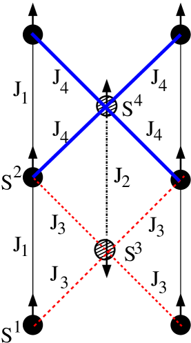
Figure 1: (Color online) Classical ferrimagnetic ground state of 2D F-AF chain. The basic magnetic unit cell comprises of three up-spins ${\bf S}_{1},{\bf S}_{2},{\bf S}_{4}$ and one down-spin ${\bf S}_{3}$. The interaction strengths $J_{1},J_{2},J_{3}$ are all positive and $J_{4}$ is the frustrated bond.

Classical Ground State: The basic model consists of alternating 1D ferro (strength $J_{1}=1$) and antiferromagnetic (strength $J_{2}=\eta_{2}J_{1}$) S=1/2 chains (along the $y$-axis). The nearest chains interact with interaction strengths $J_{3}$ ($=\eta_{3}J_{1}$) and $J_{4}$ ($=\eta_{4}J_{1}$) which are antiferromagnetic. Before discussing the excitations and quantum spin fluctuations, we first consider the ground state of our model when the spins are treated classically (mean field state). With $J_{3}=J_{4}=0$, the ground state ($G_{0}$) with broken global symmetry consists of decoupled alternating ordered F chains (S₁ and S₂ spins) and AF chains (S₃ and S₄ spins). Due to the time reversal symmetry, the F chains can be either up or down (chosen arbitrarily) and the AF chains can be in one of the two Neél states. The degeneracy of the $G_{0}$ is $2^{2M}$, where $M$ is the number of F (or AF) chains. For $J_{3}>0$ and $J_{4}=0$, if we fix the orientation of one F chain, the nearest two AF chain orientations are fixed by the $J_{3}$ bond. The neighboring F chain orientations are then fixed. In this way, we have the exact ground state $G$ as each bond takes its minimum energy value. When $\eta_{3}>0$ and $\eta_{4}<0$ (ferromagnetic), the system is not frustrated and the classical GS is a collinear ferrimagnetic state as shown in Fig. 1. However, for $\eta_{3}>0$ and $\eta_{4}>0$, spin ${\bf S}_{4}$ is frustrated. For weak frustration i.e. $\eta_{4}<<\eta_{3}$, $G$ is most likely the exact ground state and with increasing frustration ($J_{4}$) the system will undergo a phase transition to a new state which may or may not be long range ordered. One approach to attack the problem is to use the generalized Luttinger Tisza method [Luttinger and Tisza, 1951] first proposed by Lyons and Kaplan.Lyons and Kaplan (1960) It turns out that for our Bravais lattice with four-spin/unit cell system the calculations are quite difficult. So in the absence of the knowledge of the exact ground state for large $J_{4}$, we have used a different approach. We study the local stability of $G$ with increasing strength of the frustrating bond ($J_{4}$). As we will show later, depeding on the strength of $J_{2}/J_{1}$, there is a critical value of $J_{4}/J_{3}$ where the ground state $G$ is no longer locally stable. Thus in our current analysis of the phase diagram and excitations of the model using spin-wave theory we use $G$ as the ground state.

IV Spin-wave Theory

It is well-known that spin-wave theory is best suited to treat the dynamics of long range-ordered states in quantum spin system with large spin $S$. In the leading order (linear spin wave theory - LSWT), the excitations are magnons. When magnon-magnon interaction effects are negligible (for example for $S>>1/2$ and three dimensions), LSWT provides a very good description of the quantum spin fluctuation effects, one example being the reduction of the ordered moment in Heisenberg quantum antiferromagnets. However, for S=1/2 systems in 2D, magnon-magnon interactions are not negligible and one must incorporate higher order spin (1/S) corrections to treat the system.Igarashi (1992, 1993); Igarashi and Nagao (2005); Majumdar (2010) Even for these systems, LSWT provides qualitatively correct physics. For example, for 2D Heisenberg spin systems with nearest neighbor (NN) antiferromagnetic (AF) coupling [($J_{1},J_{2}$) model with no frustration i.e. $J_{2}=0$] on a square lattice, the ordered moment (average sublattice spin $\langle S_{z}\rangle$) reduces due to QSF from 0.5 to 0.303 as given by LSWT.Anderson (1952); Harris et al. (1971) When one includes the higher order magnon-magnon interaction effects using (1/S) expansion theory $\langle S_{z}\rangle=0.307$,Igarashi and Nagao (2005); Majumdar (2010) indicating that LSWT is very reasonable. For the general ($J_{1},J_{2}$) model, the effect of frustration is much more subtle. Frustration tends to destabilize long range order. With increase in the strength of frustration, $\langle S_{z}\rangle=0$ at a critical value of $J_{2}=J_{2c}$. LSWT gives $J_{2c}=0.38$ whereas including the magnon-magnon interaction one finds $J_{2c}=0.41$,Igarashi (1993); Majumdar (2010) again indicating the reasonableness of LSWT in providing a measure of the QSF induced reduction of the magnetization $M$. In a recent work (Ref. [Syromyatnikov and Aktersky, 2019]) results for this model is obtained using a four-spin bond operator technique where it is found that $\langle S_{z}\rangle=0.301$ for $J_{2}=0$ and $J_{2c}=0.36$, which are close to the LSWT results. We should mention here that all these method fail in the spin disordered state i.e. when $J_{2}>J_{2c}$.

In view of the above discussion, we opted to use LSWT to analyze the effect of QSF on the average magnetic moment and the critical strength of the frustration where the ordered moments vanish. Unlike the ($J_{1},J_{2}$) model (two sublattice with same value of the ordered moment) our 2D frustrated ($J_{1},J_{2},J_{3},J_{4}$) model has a 4-sublattice structure as shown below and different sublattice moments are affected differently by QSF.

For our analysis we only consider the parameter space $(\eta_{2},\eta_{3},\eta_{4})$ of the Hamiltonian ${\cal H}$ [Eq. (2)] where the GS is stable and is long range ordered collinear ferrimagnetic state. The spin Hamiltonian in Eq. (3) is mapped onto a Hamiltonian of interacting bosons by expressing the spin operators in terms of bosonic creation and annihilation operators $a^{\dagger},a$ for three “up” spins (spins 1, 2, and 4) and $b^{\dagger},b$ for one “down’ spin (spin 3) using the standard Holstein-Primakoff representation Holstein and Primakoff (1940)

$$S_{in}^{+i} \approx \sqrt{2S}a_{in},\;S_{in}^{-i}\approx\sqrt{2S}a_{in}^{\dagger},\;S_{in}^{zi}=S-a^{\dagger}_{in}a_{in},$$

$$S_{jn}^{+j} \approx \sqrt{2S}b_{jn}^{\dagger},\;S_{jn}^{-j}\approx\sqrt{2S}b_{jn},\;S_{jn}^{zj}=-S+b^{\dagger}_{jn}b_{jn},$$

and expand the Hamiltonian [Eq. (3)] perturbatively in powers of $1/S$ keeping terms only up to the quadratic terms. The resulting quadratic Hamiltonian is given as:

$${\cal H}=E_{\rm cl}+{\cal H}_{0}+\cdots,$$ (4)

where

$$E_{\rm cl}=-2J_{1}NS^{2}\big{[}1+\eta_{2}+2(\eta_{3}-\eta_{4})\big{]}$$ (5)

is the classical GS energy and

$${\cal H}_{0}=2SJ_{1}\sum_{{\bf k}\in{\rm BZ}}\Big{[}(1+\eta_{3}-\eta_{4})\Big{(}a^{(1)\dagger}_{\bf k}a_{\bf k}^{(1)}+a^{(2)\dagger}_{\bf k}a_{\bf k}^{(2)}\Big{)}$$

$$-\gamma_{y}\Big{(}a^{(1)}_{\bf k}a_{\bf k}^{(2)\dagger}+a^{(1)\dagger}_{\bf k}a_{\bf k}^{(2)}\Big{)}+(\eta_{2}-2\eta_{4})a^{(4)\dagger}_{\bf k}a_{\bf k}^{(4)}$$

$$+(\eta_{2}+2\eta_{3})b^{(3)\dagger}_{-\bf k}b_{-\bf k}^{(3)}+\eta_{2}\gamma_{y}\Big{(}b^{(3)\dagger}_{-\bf k}a_{\bf k}^{(4)\dagger}+b^{(3)}_{-\bf k}a_{\bf k}^{(4)}\Big{)}$$

$$+\eta_{3}\gamma_{x}\Big{(}e^{ik_{y}b/4}a^{(1)\dagger}_{\bf k}b_{-\bf k}^{(3)\dagger}+e^{-ik_{y}b/4}a^{(2)\dagger}_{\bf k}b_{-\bf k}^{(3)\dagger}+h.c.\Big{)}$$

$$+\eta_{4}\gamma_{x}\Big{(}e^{-ik_{y}b/4}a^{(1)\dagger}_{\bf k}a_{\bf k}^{(4)}+e^{ik_{y}b/4}a^{(2)\dagger}_{\bf k}a_{\bf k}^{(4)}+h.c.\Big{)}\Big{]}$$ (6)

with $\gamma_{x}=\cos(k_{x}a/2)$ and $\gamma_{y}=\cos(k_{y}b/2)$.

In the absence of inter-chain coupling ($\eta_{3}=\eta_{4}=0$) the magnon spectrum can be obtained using the standard Bogoliubov transformations. Bogoliubov (1947) We find four modes for each $k_{y}\;(-\pi/b<k_{y}<\pi/b)$ independent of $k_{x}\;(-\pi/a<k_{x}<\pi/a)$: two from the F-chains ($\alpha$-branches) and two from the AF-chains (one $\alpha$ and one $\beta$). The quadratic Hamiltonian takes the following form:

$${\cal H}_{0} = \sum_{{\bf k}\in{\rm BZ}}\Big{[}\epsilon_{\bf k}^{(1)}\alpha^{(1)\dagger}_{\bf k}\alpha_{\bf k}^{(1)}+\epsilon_{\bf k}^{(2)}\alpha^{(2)\dagger}_{\bf k}\alpha_{\bf k}^{(2)}$$

$$+ \epsilon_{\bf k}^{(3)}\Big{(}\alpha^{(4)\dagger}_{\bf k}\alpha_{\bf k}^{(4)}+\beta^{(3)\dagger}_{-\bf k}\beta_{-\bf k}^{(3)}\Big{)}\Big{]}+\sum_{{\bf k}\in{\rm BZ}}\Big{(}\epsilon_{\bf k}^{(3)}-2J_{1}S\Big{)},$$

where

$$\epsilon_{\bf k}^{(1,2)}=2J_{1}S[1\mp\gamma_{y}],$$ (8a)

$$\epsilon_{\bf k}^{(3)}=2J_{2}S\sqrt{1-\gamma_{y}^{2}}=2J_{2}S|\sin(k_{y}b/2)|.$$ (8b)

The last term in Eq. (LABEL:H0special) are the LSWT corrections to the classical ground state energy $E_{\rm cl}$ in Eq. (5) for the special case $\eta_{3}=\eta_{4}=0$.

With inter-chain coupling (i.e. $\eta_{3},\eta_{4}>0$), we have not been able to find the analytical Bogoliubov transformations that transforms the bosonic spin operators to Bogoliubov quasiparticle operators that diagonalize the Hamiltonian ${\cal H}_{0}$ [Eq. (6)]. For the special case $k_{x}=\pi/a$ i.e. $\gamma_{x}=0$, we use the equation of motion method (see Appendix A) and obtain analytical solutions for the magnon dispersion which are:

$$\epsilon_{\bf k}^{(1,2)}=2J_{1}S\big{[}(1+\eta_{3}-\eta_{4})\pm\gamma_{y}\big{]},$$ (9a)

$$\epsilon_{\bf k}^{(3,4)}=2J_{1}S\big{|}(\eta_{3}+\eta_{4})\pm\sqrt{(\eta_{3}-\eta_{4}+\eta_{2})^{2}-\eta_{2}^{2}\gamma_{y}^{2}}\big{|}.$$

(9b)

When $\eta_{3}=\eta_{4}=0$ the above dispersions reduce to Eq. (8) as expected.

For the general case we use an elegant method developed by Colpa to obtain both the eigenenergies (magnon dispersions) and eigenvectors (required for the calculation of magnetization).Colpa (1978); Toth and Lake (2015) First we write the $8\times 8$ Hamiltonian [Eq. (6)] in a symmetrized form:

$${\cal H}_{0} = J_{1}S\sum_{{\bf k}\in{\rm BZ}}\sum_{i=1}^{8}X_{\bf k}^{(i)\dagger}h_{\bf k}X_{\bf k}^{(i)}$$ (10)

$$- 2J_{1}SN\left[1+\eta_{2}+2(\eta_{3}-\eta_{4})\right],$$

with the eigenvectors
$X_{\bf k}=[a_{\bf k}^{(1)},a_{\bf k}^{(2)},a_{\bf k}^{(4)},b_{\bf k}^{(3)},a_{\bf k}^{(1)\dagger},a_{\bf k}^{(2)\dagger},a_{\bf k}^{(4)\dagger},b_{\bf k}^{(3)\dagger}]$. The hermitian matrix $h_{\bf k}$ is:

$$h_{\bf k}=\begin{bmatrix}A_{1}&-B_{1}&C_{2}^{*}&0&0&0&0&C_{1}\\ -B_{1}&A_{1}&C_{2}&0&0&0&0&C_{1}^{*}\\ C_{2}&C_{2}^{*}&A_{2}&0&0&0&0&B_{2}\\ 0&0&0&A_{3}&C_{1}&C_{1}^{*}&B_{2}&0\\ 0&0&0&C_{1}^{*}&A_{1}&-B_{1}&C_{2}&0\\ 0&0&0&C_{1}&-B_{1}&A_{1}&C_{2}^{*}&0\\ 0&0&0&B_{2}&C_{2}^{*}&C_{2}&A_{2}&0\\ C_{1}^{*}&C_{1}&B_{2}&0&0&0&0&A_{3}\end{bmatrix},$$ (11)

where the constants are given in Eqs. (15).

The Cholesky decomposition has to be applied on $h_{\bf k}$ to find the complex $K$ matrix that fulfills the condition $h_{\bf k}=K^{\dagger}K$. However, the Cholesky decomposition only works if the matrix $h_{\bf k}$ is positive definite (i.e. the eigenvalues are all positive). Colpa (1978) In case the spectrum of the Hamiltonian ${\cal H}_{0}$ contains zero modes, one can add a small positive value to the diagonal of $h_{\bf k}$ to make the matrix positive “definite”. We find that the criterion for the Cholesky decomposition to work for all ${\bf k}$ is $\eta_{4}\leq\eta_{2}\eta_{3}/(\eta_{2}+2\eta_{3})$. As an example, with $\eta_{2}=3.0,\eta_{3}=0.4$, $\eta_{4}\leq\eta_{4c}$, where $\eta_{4c}=0.316$. If $\eta_{4}>\eta_{4c}$ the matrix $h_{\bf k}$ is not positive definite and the procedure fails. As we discuss later, this is precisely the same condition for the stability of the ferrimagnetic state. After obtaining the matrix $K$, we solve the eigenvalue problem of the hermitian matrix $KgK^{\dagger}$, where $g$ is a diagonal paraunitary matrix with elements $g_{ii}={\rm diag}(1,1,1,1,-1,-1,-1,-1)$. The resulting eigenvectors are then arranged in such a way that the first four diagonal elements of the diagonalized $L=U^{\dagger}KgK^{\dagger}U$ matrix are positive and the last four elements are negative. The first four positive diagonal elements correspond to the magnon dispersions.

To calculate the sublattice magnetization $m_{i}$ we first construct the diagonal matrix, $E=gL$ and then find the transformation matrix $T$, which relates the boson modes $X_{\bf k}$ with the Bogoliubov modes $\alpha_{\bf k}$ via $X_{\bf k}=T\alpha_{\bf k}$. The matrix $T$ is calculated using Toth and Lake (2015): $T=K^{-1}UE^{1/2}.$ $m_{i=1,2,4}$ of spins ${\bf S_{1}},{\bf S_{2}},{\bf S_{4}}$ are positive but $m_{3}$ for spin ${\bf S_{3}}$ is negative. So we calculate the magnitude of $m_{i=1-4}$ for each of the four sublattices using

$$|m_{i}|=0.5-|\tau_{i}|.$$ (12)

where $\tau_{i}$ are the reduction caused by QSFs:

$$|\tau_{i}|=\frac{1}{N}\sum_{{\bf k}\in{\rm BZ}}\Big{\{}T_{\bf k}{\cal D}T_{\bf k}^{\dagger}\Big{\}}_{i+4,i+4}.$$ (13)

${\cal D}$ is a diagonal matrix with $[0,0,0,0,1,1,1,1]$ as the diagonal elements. We again reiterate that the parameters $\eta_{2},\eta_{3},\eta_{4}$ are chosen such a way that the condition for the Cholesky decomposition is satisfied, i.e. $\eta_{4}\leq\eta_{4c}$.

V Magnon Dispersion and Sublattice Magnetization

V.1 Magnon Dispersion

Effects of inter-chain interaction on the magnon dispersion is displayed in Fig. 2(a-e) where for illustration we have chosen $\eta_{2}=3,\eta_{3}=0.4$ and the frustration parameter $\eta_{4}$ is increased from 0.05 to 0.315. The dispersion along $k_{y}$ (along the chains) is given for two values of $k_{x}$: $k_{x}=0$ (top two panels) and $k_{x}=\pi/a$ (bottom two panels). Also for comparison we give the dispersions for the non-interacting chains ($\eta_{3}=\eta_{4}=0$). Later we will discuss the $k_{x}$ dependence for some special modes. As expected, there are four magnon modes for each ${\bf k}$. For the non-interacting chains, there are two F-magnon modes which are split (the lower mode $\sim k_{y}^{2}$ for small $k_{y}$) and two AF-magnons which are degenerate ($\sim k_{y}$ for small $k_{y}$). In the presence of couplings (discussed below) we will (loosely) refer to these four modes as two F and two AF modes.

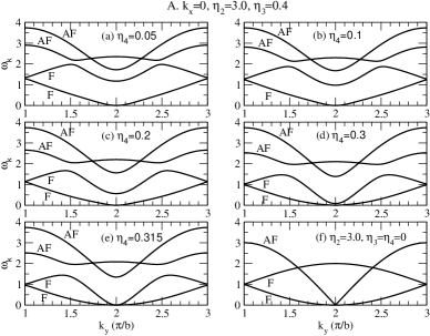
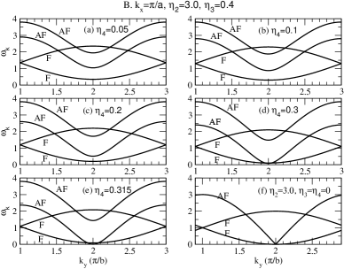
Figure 2: Magnon dispersion of the ferrimagnetic state for A. $k_{x}=0$ and B. $k_{x}=\pi/a$ [Figs. (a-e)] with $\eta_{2}=3.0,\eta_{3}=0.4$. The frustration parameter $\eta_{4}$ is varied from 0.05 (small frustration) to $\eta_{4}=0.315$. (f) Limiting case with no inter-chain coupling: the two AF-branches are degenerate, the F-branches are gapped, and the lower F-branch vanishes at $k_{y}=2\pi/b(=0)$. Note that due to 2$\pi$ periodicity $k_{y}=[-\pi/b,\pi/b]=[\pi/b,3\pi/b]$.

First we consider the case $k_{x}=\pi/a$ (bottom two panels) where the hybridization between the F and AF modes is absent (as $\gamma_{x}=0$) - so the F and AF chains interact only through effective fields. In this limit, we find from Eq. (9a) and Eq. (9b) that the F-modes get rigidly shifted upwards by $2J_{1}S(\eta_{3}-\eta_{4})$, the two degenerate AF-modes are split by $4J_{S}(\eta_{3}+\eta_{4})$, and both the modes $\sim k_{y}^{2}$. At $k_{y}=0$ the lower F-mode and the lower AF-mode are gapped, $\Delta_{\rm F}(\pi/a,0)=2J_{1}S(\eta_{3}-\eta_{4})$ and $\Delta_{\rm AF}(\pi/a,0)=2J_{1}S[\sqrt{(\eta_{2}+\eta_{3}-\eta_{4})^{2}-\eta_{2}^{2}}-(\eta_{3}+\eta_{4})]$. When the frustration parameter $\eta_{4}$ is increased towards $\eta_{3}$, there is a critical value $\eta_{4c}=\eta_{2}\eta_{3}/(\eta_{2}+2\eta_{3})<\eta_{3}$, where $\Delta_{\rm AF}(\pi/a,0)=0$ but $\Delta_{\rm F}(\pi/a,0)>0$. The ferrimagnetic GS becomes locally unstable and the system transits to a new ground state (For the parameter values we have chosen $\eta_{4c}=0.316$ - this is also the place where Cholesky decomposition fails because the matrix $h_{\bf k}$ is not positive definite). This is similar to the field induced quantum phase transition as a function of the external magnetic field for the 1D quantum ${\rm S}_{1}=1,{\rm S}_{2}=1/2$ model discussed in the introduction.Brehmer et al. (1997); Kolezhuk et al. (1999) Here the optic mode gap goes to zero at a critical field and the system undergoes a quantum phase transition from a ferrimagnetic state to some other state. This phase transition occurs in the range $\eta_{3}>\eta_{4}>\eta_{4c}$. Fig. 3 shows a schematic phase diagram in the $(\eta_{4}/\eta_{2},\eta_{3}/\eta_{2})$ space. We also note that for given $\eta_{3}$ and $\eta_{4}\leq\eta_{3}$, the strength of the exchange in the AF chains $\eta_{2}$ should be greater than a critical value $\eta_{2c}=2\eta_{3}\eta_{4}/(\eta_{3}-\eta_{4})$ for the ferrimagnetic state to be stable.

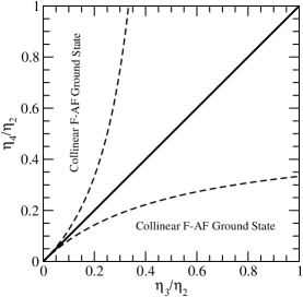
Figure 3: Phase diagram of ${\cal H}$ [Eq (2)]: normalized ${\tilde{\eta}_{4}}=\eta_{4}/\eta_{2}$ is plotted against normalized ${\tilde{\eta}_{3}}=\eta_{3}/\eta_{2}$. The dashed lines are given by the equations ${\tilde{\eta}_{4}}={\tilde{\eta}_{3}}/(1+2{\tilde{\eta}_{3}})$ (lower one) and ${\tilde{\eta}_{3}}={\tilde{\eta}_{4}}/(1+2{\tilde{\eta}_{4}})$ (upper one). They are the boundaries of the stability of the ferrimagnetic state. The solid thick line ${\tilde{\eta}_{4}}={\tilde{\eta}_{3}}$ is most likely a critical line.

For $k_{x}=0$, the picture is qualitatively similar, but with two fundamental differences resulting from hybridization between ferro and antiferro chain excitations. First, the lower F-mode goes to zero when $k_{y}\rightarrow 0$ as it should for the Goldstone mode. However the dispersion for large $k_{y}$ differs qualitatively from the non-interacting chains. Second, hybridization between the upper F-mode and the lower AF-mode opens up a hybridization gap at a finite $k_{y}$ and the size of the gap increases with $\eta_{4}$. However, as for the $(k_{x},k_{y})=(\pi/a,0)$ the gap $\Delta_{\rm AF}(\pi/a,0)\rightarrow 0$ as $\eta_{4}\rightarrow\eta_{4c}$. In fact $\Delta_{\rm AF}(k_{x},0)\rightarrow 0$ for all values of $0\leq k_{x}\leq\pi/a$ for $\eta_{4}\rightarrow\eta_{4c}$. In Fig. 4B we show the $k_{x}$ dependence of $\Delta_{\rm AF}(k_{x},0)$ for three different values of the frustration parameter $\eta_{4}$. Also we show in Fig. 4A the $k_{x}$ dependence of $\Delta_{\rm F}(k_{x},0)$. This suggests that the chains become dynamically decoupled and since the decoupled AF chains are spin liquids without any long range order, the system goes from an ordered state to a spin disordered state when $\eta_{4}>\eta_{4c}$. Exact calculations will tell us about the precise nature of the ground state for $\eta_{4c}<\eta_{4}<\eta_{3}$.

Figure 4: Gaps for F-mode ($\Delta_{\rm F}$) and AF-mode ($\Delta_{\rm AF}$) with increase in $k_{x}$ for $k_{y}=0$ with $\eta_{2}=3.0,\eta_{3}=0.3$ and three different values of $\eta_{4}=0.05,0.2,$ and 0.315.

V.2 Sublattice Magnetization

Following Colpa’s method we have calculated the sublattice magnetizations $m_{i}$ for the four sites. We have checked that the sum of the reduction in the four sublattice moments due to quantum fluctuations, $\sum_{i=1}^{4}\tau_{i}=0$, which results in the total magnetic moment equal to one as expected. This is equivalent to the results obtained for S${}_{1}=1$, S${}_{2}=1/2$ 1D quantum ferrimagnetic state for which the total magnetization/unit cell is equal to 0.5. Next we discuss the effect of frustration on the quantum fluctuation induced reduction of the long-range ordered moments for the four different spins of the unit cell. In the absence of interchain coupling [Fig. 1], $m_{1}=\langle S_{1z}\rangle=m_{2}=\langle S_{2z}\rangle=0.5$ and $m_{3}=\langle S_{3z}\rangle=-m_{4}=\langle S_{4z}\rangle=0$ (due to quantum spin fluctuation in 1D AF). When we turn on $\eta_{3}$, its effect is to produce an ordering field at the ${\bf S}_{3}$ sites and order them in the direction opposite to the F-chain spins. The intra AF chain interaction orders the ${\bf S}_{4}$ spins parallel to the F-chain spins, resulting in a 2D ferrimagnetic ground state. If $\eta_{2}\ll\eta_{3}$ then the system will be more 2D, $m_{1}=m_{2}\cong 0.5$, and $m_{3},m_{4}$ will be non-zero with the magnitude of $m_{3}$ larger than $m_{4}$. On the other hand if $\eta_{2}\gg\eta_{3}$, then intra-chain AF bonds will dominate, making the AF chains nearly decoupled and the LRO in the AF chains will be small, $m_{4}\approx-m_{3}\ll 0.5$.

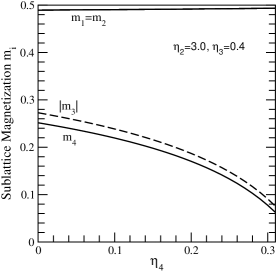
Figure 5: Magnitude of sublattice magnetizations, $m_{i}$, for $\eta_{2}=3.0,\eta_{3}=0.4$ as function of $\eta_{4}$. Magnetizations for the two degenerate ($m_{1}=m_{2}$) ferro-modes (solid) corresponding to spins 1 and 2 slowly increase as $\eta_{4}$ is increased. Magnetizations $m_{3},m_{4}$ for spins 3 (dashed) and 4 (solid) decrease due to the increase in quantum fluctuations with increase in $\eta_{4}$. The ferrimagnetic ground state is stable in the parameter space $(\eta_{2},\eta_{3},\eta_{4})$ as long as $\eta_{3}>\eta_{4}$ and $\eta_{4}\leq\eta_{4c}$, where $\eta_{4c}=0.316$ for $\eta_{2}=3.0,\eta_{3}=0.4$.

In Fig. 5, we show how the ordered moments change with the increasing strength of the frustrated bond $\eta_{4}$ for specific values of $\eta_{2}=3.0$ and $\eta_{3}=0.4$. As $\eta_{4}$ approaches the critical value 0.316 the magnetization of the AF chain decreases but remains finite ($|m_{3}|\sim 0.07,|m_{4}|\sim 0.06$) just before quantum phase transition to other ground state within LSWT. This is in contrast to what happens in the ($J_{1},J_{2}$) model where as $J_{2}$ approaches $J_{c}$ ($J_{c1}$ from the Neél state and $J_{c2}$ from the CAF state), the sublattice magnetization goes to zero.

Finally, in Fig. 6(a-b), we show the $\eta_{2}$ dependence of the magnitudes of the four order parameters $m_{i}$ ($i=1..4$) for $\eta_{3}=0.4$ for two fixed values of the frustrated interchain bond $\eta_{4}$. For our assumed collinear ferrimagnetic ground state $\eta_{3}>\eta_{4}$ and $\eta_{2}>\eta_{2}^{c}$. For $\eta_{3}=0.4,\eta_{4}=0.1$, the critical value of $\eta_{2}^{c}$ is =0.27 and for $\eta_{4}=0.2$, $\eta_{2c}=0.80$.

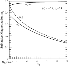
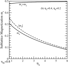
Figure 6: (a-b) Magnitude of sublattice magnetizations, $m_{i}$ for $\eta_{3}=0.4$, $\eta_{4}=0.1$ (Fig. a) and $0.2$ (Fig. b) as function of $\eta_{2}$. The ferrimagnetic ground state is stable for $\eta_{2}\geq\eta_{2c}$ where $\eta_{2c}=0.27$ for $\eta_{4}=0.1$ and $\eta_{2}^{c}=0.80$ for $\eta_{4}=0.2$. Ferro modes (solid) corresponding to spins 1 and 2 are degenerate ($m_{1}=m_{2}$). Magnetizations $m_{3},m_{4}$ for spins 3 (dashed) and 4 (solid) decrease due to the increase in quantum fluctuations with increase in $\eta_{2}$.

For small $\eta_{2}$ i.e $\eta_{2}\ll\eta_{3}$, $m_{1}=m_{2}=|m_{3}|\sim 0.46$ and $m_{4}\sim 0.38$, a reduction from 0.5 by 8% and 24% respectively. The small antiferromagnetic coupling between spins of the AF-chain induces a relatively large value of the moment at the site 4. When $\eta_{2}$ increases the QSF in the AF-chain reduces the moments at sites 3 and 4. Notice that site 3 still has a larger moment (in magnitude) than at site 4. For large $\eta_{2}$ values, say $\eta_{2}\sim 6$, ferro chain spins have moments $\sim 0.495$, whereas AF chain spins have moments of magnitude $\sim 0.14(>0)$ due to small stabilizing interchain coupling $\eta_{3}=0.4$ [Fig. 6(a)]. Increasing the strength of the frustrated bond $\eta_{4}$ essentially decouples the chains. For example with $\eta_{4}=0.2$, at $\eta_{2}=6.0$ ferro chains have moments close to 0.5 and AF-chains have moments of magnitude $~{}0.08$ [Fig. 6(b)]. For $\eta_{2}<\eta_{2c}$, the system is most likely a spin liquid state without LRO.

VI Conclusions

In summary, we have proposed a 2D frustrated Heisenberg model consisting of alternating 1D ferro ($J_{1}$) and antiferro ($J_{2}$) chains which interact with alternating frustrated ($J_{4}$) and unfrustrated ($J_{3}$) bonds (strengths). The ground state is a long range ordered ferrimagnetic state in certain region of the parameter space. Analysis using linear spin wave theory suggests that the system undergoes a quantum phase transition to a quantum disordered phase with increasing strength of $\eta_{4}$, similar to the classic 2D ($J_{1},J_{2}$) model. However in contrast to the ($J_{1},J_{2}$) model, the sublattice magnetizations of the AF chains do not vanish at the critical value $\eta_{4c}$, similar to the 1D ${\rm S}_{1}=1,{\rm S}_{2}=1/2$ model of a quantum ferrimagnet. The exact nature of the phase transition, the nature of the GS above $\eta_{4c}$, and whether the order parameter vanishes at the transition should be explored by other theoretical and numerical techniques.

VII Acknowledgment

SDM would like to thank Dr. Xianglin Ke for stimulating discussions.

Appendix A Equation of Motion Method

With inter-chain coupling (i.e. $\eta_{3},\eta_{4}>0$), we are unable to find the the Bogoliubov transformations that diagonalizes the Hamiltonian in Eq. (6). Thus we opt for another way - the canonical equation of motion method to obtain the magnon dispersion.Diep (2004) The various commutators that are needed for the canonical equation of motion method are:

$$\big{[}a_{\bf k}^{(1)},{\cal H}_{0}/2J_{1}S\big{]} = A_{1}a_{\bf k}^{(1)}-B_{1}a_{\bf k}^{(2)}+C_{1}b_{\bf k}^{(3)\dagger}+C_{2}^{*}a_{\bf k}^{(4)},$$ (14a)

$$\big{[}a_{\bf k}^{(2)},{\cal H}_{0}/2J_{1}S\big{]} = A_{1}a_{\bf k}^{(2)}-B_{1}a_{\bf k}^{(1)}+C_{1}^{*}b_{\bf k}^{(3)\dagger}+C_{2}a_{\bf k}^{(4)},$$ (14b)

$$\big{[}a_{\bf k}^{(4)},{\cal H}_{0}/2J_{1}s\big{]} = A_{2}a_{\bf k}^{(4)}+B_{2}b_{\bf k}^{(3)\dagger}+C_{2}a_{\bf k}^{(1)}+C_{2}^{*}a_{\bf k}^{(2)},$$ (14c)

$$\big{[}b_{\bf k}^{(3)\dagger},{\cal H}_{0}/2J_{1}s\big{]} = -A_{3}b_{\bf k}^{(3)\dagger}-B_{2}a_{\bf k}^{(4)}-C_{1}^{*}a_{\bf k}^{(1)}-C_{1}a_{\bf k}^{(2)},$$ (14d)

$$\big{[}a_{\bf k}^{(1)\dagger},{\cal H}_{0}/2J_{1}S\big{]} = -A_{1}a_{\bf k}^{(1)\dagger}+B_{1}a_{\bf k}^{(2)\dagger}-C_{1}^{*}b_{\bf k}^{(3)}-C_{2}a_{\bf k}^{(4)\dagger},$$ (14e)

$$\big{[}a_{\bf k}^{(2)\dagger},{\cal H}_{0}/2J_{1}S\big{]} = -A_{1}a_{\bf k}^{(2)\dagger}+B_{1}a_{\bf k}^{(1)\dagger}-C_{1}b_{\bf k}^{(3)}-C_{2}^{*}a_{\bf k}^{(4)\dagger},$$ (14f)

$$\big{[}a_{\bf k}^{(4)\dagger},{\cal H}_{0}/2J_{1}s\big{]} = -A_{2}a_{\bf k}^{(4)\dagger}-B_{2}b_{\bf k}^{(3)}-C_{2}^{*}a_{\bf k}^{(1)\dagger}-C_{2}a_{\bf k}^{(2)\dagger},$$ (14g)

$$\big{[}b_{\bf k}^{(3)},{\cal H}_{0}/2J_{1}s\big{]} = A_{3}b_{\bf k}^{(3)}+B_{2}a_{\bf k}^{(4)\dagger}+C_{1}a_{\bf k}^{(1)\dagger}+C_{1}^{*}a_{\bf k}^{(2)\dagger},$$ (14h)

where

$$A_{1} = (1+\eta_{3}-\eta_{4}),\;A_{2}=(\eta_{2}-2\eta_{4}),$$ (15a)

$$A_{3} = (\eta_{2}+2\eta_{3}),\;B_{1}=\gamma_{y},\;B_{2}=\eta_{2}\gamma_{y},$$ (15b)

$$C_{1} = \eta_{3}\gamma_{x}e^{ik_{y}b/4},\;C_{2}=\eta_{4}\gamma_{x}e^{ik_{y}b/4}.$$ (15c)

We notice that the first four commutators [Eqs. (14a) - (14d)] are decoupled from the second four commutators [Eqs. (14e) - (14h)]. With the basis vectors $X_{\bf k}=(a_{\bf k}^{(1)},a_{\bf k}^{(2)},a_{\bf k}^{(4)},b_{\bf k}^{(3)\dagger})$, the canonical equation of motion can be deduced from the Hamiltonian in Eq. (6) in the following way:

$$\Big{[}X_{\bf k}^{(i)},\frac{{\cal H}_{0}}{2J_{1}S}\Big{]}=i\frac{dX_{\bf k}^{(i)}}{dt}=g\omega_{\bf k}^{(i)}X_{\bf k}^{(i)}.$$ (16)

In Eq. (16) $g$ is a $4\times 4$ diagonal matrix with $g_{ii}=(1,1,1,-1)$ in the diagonal elements. The eigenvalues, $\omega_{\bf k}^{(i)}$ are obtained by solving the determinant:

$$\begin{vmatrix}(A_{1}-\omega_{\bf k}^{(i)})&-B_{1}&C_{2}&C_{1}^{*}\\ -B_{1}&(A_{1}-\omega_{\bf k}^{(i)})&C_{2}^{*}&C_{1}\\ C_{2}^{*}&C_{2}&(A_{2}-\omega_{\bf k}^{(i)})&B_{2}\\ C_{1}&C_{1}^{*}&B_{2}&(A_{3}+\omega_{\bf k}^{(i)})\end{vmatrix}=0.$$ (17)

The above determinant leads to a fourth-order polynomial:

$$\omega_{\bf k}^{4}+a\omega_{\bf k}^{3}+b\omega_{\bf k}^{2}+c\omega_{\bf k}+d=0,$$ (18)

where the coefficients are:

$$a = -2(1-2\eta_{4}),$$ (19a)

$$b = (1+\eta_{3}-\eta_{4})^{2}-4(1+\eta_{3}-\eta_{4})(\eta_{3}+\eta_{4})-(\eta_{2}+2\eta_{3})(\eta_{2}-2\eta_{4})-(1-\eta_{2}^{2})\gamma_{y}^{2}+2(\eta_{3}^{2}-\eta_{4}^{2})\gamma_{x}^{2},$$ (19b)

$$c = 2(1+\eta_{3}-\eta_{4})^{2}(\eta_{3}+\eta_{4})+2(1+\eta_{3}-\eta_{4})(\eta_{2}-2\eta_{4})(\eta_{2}+2\eta_{3})-2\eta_{2}^{2}(1+\eta_{3}-\eta_{4})\gamma_{y}^{2}-2(\eta_{3}+\eta_{4})\gamma_{y}^{2}$$ (19c)

$$- 2(1+\eta_{2}+\eta_{3}-3\eta_{4})\eta_{3}^{2}\gamma_{x}^{2}+2(1-\eta_{2}-\eta_{3}-\eta_{4})\eta_{4}^{2}\gamma_{x}^{2}-2(\eta_{3}^{2}-\eta_{4}^{2})\gamma_{x}^{2}\gamma_{y}^{2}+4\eta_{2}\eta_{3}\eta_{4}\gamma_{x}^{2}\gamma_{y}^{2},$$

$$d = -(1+\eta_{3}-\eta_{4})\Big{[}(1+\eta_{3}-\eta_{4})(\eta_{2}-2\eta_{4})(\eta_{2}+2\eta_{3})-(1+\eta_{3}-\eta_{4})\eta_{2}^{2}\gamma_{y}^{2}-2(\eta_{2}-2\eta_{4})\eta_{3}^{2}\gamma_{x}^{2}$$ (19d)

$$- 2(\eta_{2}+2\eta_{3})\eta_{4}^{2}\gamma_{x}^{2}+4\eta_{2}\eta_{3}\eta_{4}\gamma_{x}^{2}\gamma_{y}^{2}\Big{]}+(\eta_{2}-2\eta_{4})(\eta_{2}+2\eta_{3})\gamma_{y}^{2}+2(\eta_{2}-2\eta_{4})\eta_{3}^{2}\gamma_{x}^{2}\gamma_{y}^{2}+2(\eta_{2}+2\eta_{3})\eta_{4}^{2}\gamma_{x}^{2}\gamma_{y}^{2}$$

$$- \eta_{2}^{2}\gamma_{y}^{4}-4\eta_{3}^{2}\eta_{4}^{2}\gamma_{x}^{2}-4\eta_{3}\eta_{4}\gamma_{x}^{2}\gamma_{y}^{2}(\eta_{2}-\eta_{3}\eta_{4}).$$

The other set of four boson operators ($a_{k}^{(1)\dagger},a_{k}^{(2)\dagger},a_{k}^{(4)\dagger},b_{k}^{(3)}$) lead to a similar fourth order polynomial equation, but the signs before the linear and cubic terms are negative. There is thus a $\omega_{\bf k}\leftrightarrow-\omega_{\bf k}$ symmetry between the two sets of solutions. This fourth order polynomial [Eq. (18)] has to be solved numerically. The four real eigen-values can be positive or negative. If we solve the fourth order polynomial associated with the other four boson operators we will get again four real solutions which are negative of the solutions of Eq. (18). For the magnon frequencies we will consider only the four positive solutions. The diagonalized quadratic Hamiltonian in terms of new basis vectors $\alpha_{\bf k}^{(i=1..4)}$ becomes:

$${\cal H}_{0}=E_{0}+\sum_{{\bf k}\in{\rm BZ}}\sum_{i=1}^{4}\epsilon_{\bf k}^{(i)}\alpha_{\bf k}^{(i)\dagger}\alpha_{\bf k}^{(i)}.$$ (20)

$E_{0}$ contributes to the LSWT correction to the classical ground state energy.

For the special case $k_{x}=\pi/a$ i.e. $\gamma_{x}=0$ the solutions of the polynomial [Eq. (18)] can be obtained analytically. They are (we only consider the positive solutions):

$$\omega_{\bf k}^{(1,2)}=(1+\eta_{3}-\eta_{4})\pm\gamma_{y},$$ (21a)

$$\omega_{\bf k}^{(3,4)}=(\eta_{3}+\eta_{4})\pm\sqrt{(\eta_{3}-\eta_{4}+\eta_{2})^{2}-\eta_{2}^{2}\gamma_{y}^{2}},$$

and thus the energies of the magnon spectrum are:

$$\epsilon_{\bf k}^{(1,2)}=2J_{1}S\big{[}(1+\eta_{3}-\eta_{4})\pm\gamma_{y}\big{]},$$ (22a)

$$\epsilon_{\bf k}^{(3,4)}=2J_{1}S\big{|}(\eta_{3}+\eta_{4})\pm\sqrt{(\eta_{3}-\eta_{4}+\eta_{2})^{2}-\eta_{2}^{2}\gamma_{y}^{2}}\big{|}.$$

References

- Diep (2004) H. T. Diep, Frustrated Spin Systems, 1st ed. (World Scientific, Singapore, 2004).
- Lacroix et al. (2011) C. Lacroix, P. Mendels, and F. Mila, Introduction to Frustrated Magnetism, 1st ed., Vol. 164 (Springer-Verlag, Berlin, 2011).
- Sachdev (2001) S. Sachdev, Quantum Phase Transitions, 1st ed. (Cambridge University Press, Cambridge, UK, 2001).
- Anderson (1952) P. W. Anderson, Phys. Rev. 86, 694 (1952).
- Harris et al. (1971) A. B. Harris, D. Kumar, B. I. Halperin, and P. C. Hohenberg, Phys. Rev. B 3, 961 (1971).
- Igarashi (1993) J. I. Igarashi, J. Phys. Soc. Jpn. 62, 4449 (1993).
- Majumdar (2010) K. Majumdar, Phys. Rev. B 82, 144407 (2010).
- Richter et al. (2015) J. Richter, R. Zinke, and D. J. J. Farnell, Eur. Phys. J. B 88, 2 (2015).
- Bishop et al. (2008) R. F. Bishop, P. H. Y. Li, R. Darradi, and J. Richter, J. Phys.: Condens. Matter 20, 255251 (2008).
- Sandvik and Singh (2001) A. W. Sandvik and R. R. P. Singh, Phys. Rev. Lett. 86, 528 (2001).
- Isaev et al. (2009) L. Isaev, G. Ortiz, and J. Dukelsky, Phys. Rev. B 79, 024409 (2009).
- Syromyatnikov and Aktersky (2019) A. V. Syromyatnikov and A. Y. Aktersky, Phys. Rev. B 99, 224402 (2019).
- Yu and Kivelson (2020) Y. Yu and S. A. Kivelson, Phys. Rev. B 101, 1580 (2020).
- Mikeska and Kolezhuk (2008) H.-J. Mikeska and A. K. Kolezhuk, in Quantum Magnetism, Lecture Notes in Physics, Vol. 645, edited by U. Schollwck, J. Richter, D. J. Farnell, and R. F. Bishop (Springer, Berlin, Heidelberg, 2008) pp. 1 – 83.
- Chubukov et al. (1991) A. V. Chubukov, K. I. Ivanova, P. C. Ivanov, and E. R. Korutcheva, J. Phys.: Condens. Matter 3, 2665 (1991).
- Kolezhuk et al. (1997) A. K. Kolezhuk, H.-J. Mikeska, and S. Yamamoto, Phys. Rev. B 55, R3336 (1997).
- Brehmer et al. (1997) S. Brehmer, H.-J. Mikeska, and S. Yamamoto, J. Phys.: Condens. Matter 9, 3921 (1997).
- Pati et al. (1997a) S. K. Pati, S. Ramasesha, and D. Sen, Phys. Rev. B 55, 8894 (1997a).
- Pati et al. (1997b) S. K. Pati, S. Ramasesha, and D. Sen, J. Phys.: Condens. Matter 9, 8707 (1997b).
- Ivanov (1998) N. B. Ivanov, Phys. Rev. B 57, R14 024 (1998).
- Kolezhuk et al. (1999) A. K. Kolezhuk, H.-J. Mikeska, K. Maisinger, and U. Schollwck, Phys. Rev. B 59, 13 565 (1999).
- Yamamoto et al. (1998) S. Yamamoto, T. Fukui, K. Maisinger, and U. Schollwck, J. Phys.: Condens. Matter 10, 11 033 (1998).
- Maisinger et al. (1998) K. Maisinger, U. Schollwck, S. Brehmer, H.-J. Mikeska, and S. Yamamoto, Phys. Rev. B 58, R5908 (1998).
- Ivanov (2000) N. B. Ivanov, Phys. Rev. B 62, 3271 (2000).
- Ivanov (2009) N. B. Ivanov, Condensed Matter Physics 12, 435 (2009).
- Ivanov and Richter (2001) N. B. Ivanov and J. Richter, Phys. Rev. B 63, 144429 (2001).
- Lieb and Mattis (1962) E. Lieb and D. Mattis, J. Math. Phys. 3, 749 (1962).
- Zhang et al. (2020) H. Zhang, Z. Zhao, D. Gautreau, M. Raczkowski, A. Saha, V. O. Garlea, H. Cao, T. Hong, H. O. Jeschke, S. D. Mahanti, T. Birol, F. F. Assad, and X. Ke, Phys. Rev. Lett. 125, 037204 (2020).
- Luttinger and Tisza (1951) J. M. Luttinger and L. Tisza, Phys. Rev. 70, 954 (1951).
- Lyons and Kaplan (1960) D. H. Lyons and T. A. Kaplan, Phys. Rev. 120, 1580 (1960).
- Igarashi (1992) J. I. Igarashi, Phys. Rev. B 46, 10 763 (1992).
- Igarashi and Nagao (2005) J. I. Igarashi and T. Nagao, Phys. Rev. B 72, 014403 (2005).
- Holstein and Primakoff (1940) T. Holstein and H. Primakoff, Phys. Rev. B 58, 1098 (1940).
- Bogoliubov (1947) N. N. Bogoliubov, J. Phys. (USSR) 11, 23 (1947).
- Colpa (1978) J. Colpa, Physica 93A, 327 (1978).
- Toth and Lake (2015) S. Toth and B. Lake, J. Phys.: Condens. Matter 27, 166002 (2015).