$Z_{c}$ -like spectra from QCD Laplace sum rules at NLO

Abstract

We present a global analysis of the observed $Z_{c},~{}Z_{cs}$ and future $Z_{css}$-like spectra using (inverse) Laplace Sum Rule (LSR) within stability criteria. Integrated compact QCD expressions of the LO spectral functions up to dimension-six condensates are given. Next-to-Leading Order (NLO) factorized perturbative contributions are included. We re-emphasize the importance to include PT radiative corrections (though numerically small) for heavy quark sum rules in order to justify the (ad hoc) definition and value of the heavy quark mass used frequently at LO in the literature. We also demonstrate that, contrary to a qualitative large $N_{c}$-counting, the two-meson scattering contributions to the four-quark spectral functions are numerically negligible confirming the reliability of the LSR predictions. Our results are summarized in Tables 3 to 6. The $Z_{c}(3900)$ and $Z_{cs}(3983)$ spectra are well reproduced by the ${\cal T}_{c}(3900)$ and ${\cal T}_{cs}(3973)$ tetramoles (superposition of quasi-degenerated molecules and tetraquark states having the same quantum numbers and with almost equal couplings to the currents). The $Z_{c}$(4025) or $Z_{c}$(4040) state can be fitted with the $D^{*}_{0}D_{1}$ molecule having a mass 4023(130) MeV while the $Z_{cs}$ bump around 4.1 GeV can be likely due to the $D^{*}_{s0}D_{1}\oplus D^{*}_{0}D_{s1}$ molecules. The $Z_{c}(4430)$ could be a radial excitation of the $Z_{c}(3900)$ weakly coupled to the current, while all strongly coupled ones are in the region $(5634\sim 6527)$ MeV. The double strange tetramole state ${\cal T}_{css}$ which one may identify with the future $Z_{css}$ is predicted to be at 4064(46) MeV. It is remarkable to notice the regular mass-spliitings of the tetramoles due to $SU(3)$ breakings : $M_{{\cal T}_{cs}}-M_{{\cal T}_{c}}\approx M_{{\cal T}_{css}}-M_{{\cal T}_{cs}}\simeq(73\sim 91)$ MeV.

I Introduction

Beyond the successful quark model of Gell-Mann GELL and Zweig ZWEIG , Rossi and Veneziano have introduced the four-quark states within the string model ROSSI in order to describe baryon-antibaryon scattering, while Jaffe JAFFE1 has introduced them within the bag models for an attempt to explain the complex structure of the $I=1,0$ light scalar mesons (see also ISGUR ; ACHASOV ; THOOFT ).

In earlier papers, QSSR has been used to estimate the $I=0$ light scalar mesons ($\sigma,f_{0},$) masses and widths LATORRE assumed to be four-quark states. However, the true nature of these states remains still an open question as they can be well interpreted as glueballs/gluonia VENEZIA ; SNG ; OCHS ; MENES3 .

After the recent discovery of many exotic XYZ states beyond the quark model found in different accelerator experiments , there was a renewed interest on the four-quarks and molecule states for attempting to explain the properties of these new exotic states .

In previous works HEP18 ; SU3 ; MOLE16 , we have systematically extracted the couplings and masses of the $XYZ$ states using QCD spectral sum rules (QSSR) à la Shifman-Vainshtein-Zakharov (SVZ) SVZa ; ZAKA   where the N2LO factorized perturbative and QCD condensates up to dimension-six in the Operator Product Expansion (OPE) corrections have been included . In so doing, we have used the inverse Laplace transform (LSR) BELLa ; BECCHI ; SNR version of QSSR within stability criteria where we have emphasized the importance of the PT corrections for giving a meaning on the input heavy quark mass value which plays an important role in the analysis, though these corrections are numerically small, within the $\overline{MS}$-scheme.

More recently, we have applied the LSR for interpreting the new states around (6.2-6.9) GeV found by the LHCb-group LHCb1 to be a doubly/fully hidden-charm molecules $(\bar{Q}Q)(Q\bar{Q})$ and $(\bar{Q}\bar{Q})(QQ)$ tetraquarks states 4Q , while the new states found by the same group from the $DK$ invariant mass LHCb3 have been interpreted by a $0^{+}$ and $1^{-}$ tetramoles (superposition of almost degenerate molecules and tetraquark states having the same quantum numbers and couplings) slightly mixed with their radial excitations DK .

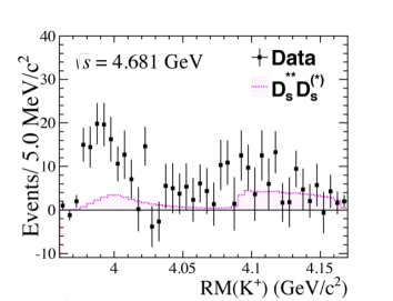
Figure 1: $K^{+}$ recoil-mass at $\sqrt{s}=4.681$ GeV after background subtractions from BESIII BES .

In this paper, we pursue the analysis using LSR by studying the recent data from BESIII where the $K^{+}$ recoil or invariant $D^{*}_{s}D\oplus D^{*}D_{s}$ mass (see Fig. 1) BES is a good $Z_{cs}(1^{+})$-like state candidate. A narrow peak is experimentally found at (in units of MeV):

$$M=(3982.5^{+1.8}_{-2.6}\pm 2.1),~{}~{}\Gamma=(12.8^{+5.3}_{-4.4}\pm 3.0).$$ (1)

II The Inverse Laplace sum rules

II.1 The QCD molecule and tetraquarks currents

We shall be concerned with the QCD local currents ${\cal O}^{\mu}_{H}(x)$ of dimension-six given in Table 1 for $1^{+}$ axial-vector molecules and tetraquarks where $q\equiv u,s$. $b$ is a free mixing parameter where its optimal value was found to be zero MOLE16 ; SU3 .

Molecules	Currents
$D^{*}_{q}D$	$(\bar{c}\gamma_{\mu}q)(\bar{u}\,i\gamma_{5}c)$
$D^{*}D_{q}$	$(\bar{u}\gamma_{\mu}c)(\bar{c}\,i\gamma_{5}q)$
$D^{*}_{q0}D_{1}$	$(\bar{c}q)(\bar{u}\gamma_{\mu}\gamma_{5}c)$
$D^{*}_{0}D_{q1}$	$(\bar{u}c)(\bar{c}\gamma_{\mu}\gamma_{5}q)$
$D^{*}_{s}D_{s}$	$(\bar{c}\gamma_{\mu}s)(\bar{s}\,i\gamma_{5}c)$
$D^{*}_{s0}D_{1s}$	$(\bar{c}s)(\bar{s}\gamma_{\mu}\gamma_{5}c)$
Tetraquarks	Currents
$A_{cq}$	$\epsilon_{ijk}\epsilon_{mnk}\big{[}(q^{T}_{i}\,C\gamma_{5}\,c_{j})(\bar{u}_{m}\gamma_{\mu}C\,\bar{c}_{n}^{T})$
	$\,+b\,(q^{T}_{i}\,C\,c_{j})(\bar{u}_{m}\gamma_{\mu}\gamma_{5}C\,\bar{c}_{n}^{T})\big{]}$
$A_{css}$	$\epsilon_{ijk}\epsilon_{mnk}\big{[}(s^{T}_{i}\,C\gamma_{5}\,c_{j})(\bar{s}_{m}\gamma_{\mu}C\,\bar{c}_{n}^{T})$
	$\,+b\,(s^{T}_{i}\,C\,c_{j})(\bar{s}_{m}\gamma_{\mu}\gamma_{5}C\,\bar{c}_{n}^{T})\big{]}$

Table 1: $(1^{+})$ molecules and tetraquarks currents ($q\equiv u,s$).

The appropriate $1^{+}$ hadron ${\cal H}$ couples to the current as :

$$\langle 0|{\cal O}^{\mu}_{\cal H}(x)|{\cal H}\rangle=f_{\cal H}M_{\cal H}^{5}\epsilon^{\mu}$$ (2)

where $f_{\cal H}$ is the hadron decay constant analogue to $f_{\pi}$ and $\epsilon^{\mu}$ is the axial-vector polarisation. In general, the four-quark operators mix under renormalization and acquire anomalous dimensions SNTARRACH . In the present case where the interpolating currents are constructed from bilinear (pseudo)scalar currents, the anomalous dimension can be transfered to the decay constants as :

$$f_{\cal H}(\mu)=\hat{f}_{\cal H}\left(-\beta_{1}a_{s}\right)^{2/\beta_{1}}(1-k_{f}\,a_{s}),$$ (3)

where : $\hat{f}_{\cal H}$ is the renormalization group invariant coupling and $-\beta_{1}=(1/2)(11-2n_{f}/3)$ is the first coefficient of the QCD $\beta$-function for $n_{f}$ flavours. $a_{s}\equiv(\alpha_{s}/\pi)$ is the QCD coupling. $k_{f}=1.014$ for $n_{f}=4$ flavours.

II.2 Form of the sum rules

We shall work with the Finite Energy version of the QCD Inverse Laplace sum rules (LSR) and their ratios :

$${\cal L}^{c}_{n}(\tau,\mu) = \int_{t_{0}}^{t_{c}}dt~{}t^{n}~{}e^{-t\tau}\frac{1}{\pi}\mbox{Im}~{}\Pi^{(1)}_{\cal H}(t,\mu)~{},$$

$${\cal R}^{c}_{n}(\tau) = \frac{{\cal L}^{c}_{n+1}}{{\cal L}^{c}_{n}},$$ (4)

where $m_{c}$ is the charm quark mass, $\tau$ is the LSR variable, $n=0,...$ is the degree of moments, $t_{0}$ is the quark/hadronic threshold. $t_{c}$ is the threshold of the “QCD continuum” which parametrizes, from the discontinuity of the Feynman diagrams, the spectral function ${\rm Im}\,\Pi^{(1)}_{\cal H}(t,m_{c}^{2},\mu^{2})$ where $\Pi^{(1)}_{\cal H}(t,m_{c}^{2},\mu^{2})$ is the transverse scalar correlator corresponding to a spin one hadron :

$$\Pi^{\mu\nu}_{\cal H}(q^{2}) = i\int d^{4}x~{}e^{-iqx}\langle 0|{\cal T}{\cal O}^{\mu}_{\cal H}(x)\left({\cal O}^{\nu}_{\cal H}(0)\right)^{\dagger}|0\rangle$$ (5)

$$\equiv -\left(g^{\mu\nu}-\frac{q^{\mu}q^{\nu}}{q^{2}}\right)\Pi^{(1)}_{\cal H}(q^{2})+\frac{q^{\mu}q^{\nu}}{q^{2}}\Pi^{(0)}_{\cal H}(q^{2})$$

III QCD two-point function

Using the SVZ SVZa Operator Product Expansion (OPE), we give in the Appendix the QCD expressions to lowest order (LO) of the two-point correlators associated to the currents given in Table 1 up to dimension $d=6$ condensate contributions.

III.1 LO perturbative (PT) and $1/N_{c}$ counting

Motivated by the criticisms raised in Ref. LUCHA0 based on the large $N_{c}$-limit which state that the non-factorized contribution of the two-point correlator starts at order $\alpha_{s}^{2}$ and that the non-resonant (scattering states) dominate the sum rules, we check explicitly these statements for finite $N_{c}$here and in the following subsection C, which we complete in Section X by comparing the $D^{*}D$ molecule resonance and the non-resonating $D^{*}$ and $D$ channels contributions to the sum rule.

The LO perturbative contributions are given by the diagrams in Fig. 2. Explicit evaluations of the Trace appearing in the two-point function indicates that the lowest order (LO) PT contribution behaves like $N_{c}^{2}$ (or $2N^{2}_{c}(1-1/N_{c})$ if the current has an $\epsilon$-tensor like the one in Table 1 where the $1/N_{c}$ term arises from the $\epsilon$-contraction) as expected from large $N_{c}$.

However, non-factorised contribution appears at LO both from PT and condensate contributions when one has two or more identical quark flavours because one has more possibilities to do the Wick’s contraction . Moreover, some care has to be taken when applying the large $N_{c}$ analysis to the case of baryons and tetraquark states with string junctions ROSSI  .

a)

                            $N_{c}^{2}$ or $N_{c}^{2}(1-1/N_{c})$

b)

              $N_{c}^{2}$    +    $N_{c}$

Figure 2: LO PT contributions to the spectral function: a) factorised; b) factorised $\oplus$ non-factorised.

$N_{c}$

Figure 3: LO eye diagram.

III.2 The LO $d\leq 6$ condensates contributions

The QCD condensates entering in the analysis are the light quark condensate $\langle\bar{q}q\rangle$ and the $SU(3)$-breaking parameter $\kappa\equiv\langle\bar{s}s\rangle/\langle\bar{q}q\rangle$, the gluon condensates $\langle\alpha_{s}G^{2}\rangle\equiv\langle\alpha_{s}G^{a}_{\mu\nu}G_{a}^{\mu\nu}\rangle$ and $\langle g^{3}G^{3}\rangle\equiv\langle g^{3}f_{abc}G^{a}_{\mu\nu}G^{b}_{\nu\rho}G^{c}_{\rho\mu}\rangle$, the mixed quark-gluon condensate $g\langle\bar{q}Gq\rangle\equiv{\langle\bar{q}g\sigma^{\mu\nu}(\lambda_{a}/2)G^{a}_{\mu\nu}q\rangle}=M_{0}^{2}\langle\bar{q}q\rangle$ and the four-quark condensate $\rho\langle\bar{q}q\rangle^{2}$, where $\rho\simeq(3\sim 4)$ indicates the deviation from the four-quark vacuum saturation. Their different contributions within the SVZ expansion to LO are shown in Figs. 4 to 8.

Unlike often used in the literature, we have not included higher dimension $d\geq 8$ condensates contributions  due to our poor knowledge of their size. Indeed, a violation of the vacuum saturation for the four-quark condensates SNTAU ; JAMI2a ; JAMI2c ; LNT ; LAUNERb has been already noticed in different light quark channels. In addition, the mixing of different four-quark condensates under renormalization SNTARRACH does not also favour the vacuum saturation estimate. On the other, the inaccuracy of a simple dilute gas instanton estimate SVZa ; SHURYAK1 has been also observed from the phenomenological estimate of high-dimension gluon condensates SNH10 ; SNH11 ; SNH12 .

Figure 4: $\langle\bar{q}q\rangle$ quark condensate.

Figure 5: $\langle\alpha_{s}G^{2}\rangle$ gluon condensate.

Figure 6: $g\langle\bar{q}Gq\rangle$ mixed quark-gluon condensate.

Figure 7: $\langle g^{3}G^{3}\rangle$ triple gluon condensate.

Figure 8: $\rho\langle\bar{\psi}\psi\rangle^{2}$ four-quark condensate.

III.3 Convolution representation and Matching

We have explicitely proved in our previous papers HEP18 ; SU3 ; MOLE16 ; 4Q ; DK that the non-factorized contribution to the four-quark correlator which appears at lowest order $\alpha_{s}^{0}$ of PT QCD to order in $1/N_{c}$ (but not to order $\alpha_{s}^{2}$ as claimed by LUCHA0 ), gives numerically negligible contribution to the sum rule. Therefore, we can consider that the molecule /tetraquark two-point spectral function is well approximated by the convolution of the two ones built from two quark bilinear currents (factorization) as illustrated in Fig. 9 where the diagrams in the two sides of Fig. 9 are of the order $N_{c}^{2}$.

Figure 9: The four-quark spectral function as a convolution of two quark bilinear ones (see Eq. 8). The black region means perturbative $\oplus$ non-perturbative contributions.

In order to fix the matching factor $k^{2}$, we consider the example of the $D^{*}D$ molecule current where the QCD expression is given in the Appendix. The bilinear currents and the corresponding spectral functions entering in the RHS of Fig. 9 are :

$$J^{P,S}(x) \equiv \bar{c}[i\gamma_{5},1]c~{}\rightarrow~{}\frac{1}{\pi}{\rm Im}\,\psi^{P,S}(t)\sim\frac{3}{8\pi^{2}}$$

$$J^{V,A}(x) \equiv \bar{c}[\gamma_{\mu},\gamma_{\mu}\gamma_{5}]c~{}\rightarrow~{}\frac{1}{\pi}{\rm Im}\,\psi^{V,A}(t)\sim\frac{1}{4\pi^{2}}~{},$$ (6)

in the limit where $m_{c}^{2}\ll t$. In this way, we obtain, for a spin 1 state, the convolution integral PICH ; SNPIVO ; HAGIWARA :

$$\frac{1}{\pi}{\rm Im}\,\Pi_{\cal H}(t) =\theta[t-(\sqrt{t_{10}}+\sqrt{t_{20}})^{2}]\left(\frac{k}{4\pi}\right)^{2}t^{2}\int_{t_{10}}^{(\sqrt{t}-\sqrt{t_{20}})^{2}}dt_{1}\times$$

$$\int_{t_{20}}^{(\sqrt{t}-\sqrt{t_{1}})^{2}}dt_{2}~{}2\,\lambda^{3/2}\left(\frac{t_{1}}{t},\frac{t_{2}}{t}\right)\frac{1}{\pi}{\rm Im}\,\psi^{S,P}(t_{1})\frac{1}{\pi}{\rm Im}\,\psi^{A,V}(t_{2}):$$

with the phase space factor:

$${\footnotesize\lambda\left(\frac{t_{1}}{t},\frac{t_{2}}{t}\right)=\left(1-\frac{\left(\sqrt{t_{1}}-\sqrt{t_{2}}\right)^{2}}{t}\right)\left(1-\frac{\left(\sqrt{t_{1}}+\sqrt{t_{2}}\right)^{2}}{t}\right).}$$ (8)

$\sqrt{t_{10}}$ and $\sqrt{t_{20}}$ are the quark / hadronic thresholds and $m_{c}$ is the on-shell / pole perturbative charm quark mass.

The appropriate $k$-factor which matches this convolution representation with the direct perturbative calculation of the molecule spectral function given in the appendix is  :

$$k^{2}=\frac{5}{3\times 2^{6}}~{},$$ (9)

which comes from the dynamics of the Feynman diagram calculations and which is missed in a standard large $N_{c}$-results of LUCHA . Related phenomenology will be discussed in Section X.

III.4 NLO PT corrections to the Spectral functions

We extract the next-to-leading (NLO) perturbative (PT) corrections by approximating the molecule /tetraquark two-point spectral function with the convolution of the two ones built from two quark bilinear currents (factorization) illustrated in Fig. 10.

Figure 10: NLO factorised PT contribution to the spectral function.

The NLO perturbative expressions of the bilinear unequal masses (pseudo)scalar and (axial)-vector spectral functions are known in the literature BROAD ; RRY ; SNB1 ; SNB2 ; CHET1 ; PIVOSU3 .

III.5 From the On-shell to the $\overline{MS}$-scheme

We transform the pole mass $m_{c}$ to the running mass $\overline{m}_{c}(\mu)$ using the known relation in the $\overline{MS}$-scheme to order $\alpha_{s}^{2}$ SNB1 ; SNB2

$$m_{c}=\overline{m}_{c}(\mu)\Big{[}1+\frac{4}{3}a_{s}\\ +a_{s}\mbox{Log}{\frac{\mu^{2}}{m_{c}^{2}}}+{\cal O}(a_{s}^{2})\Big{]}.$$

In the following, we shall use $n_{f}$=4 total number of flavours for the numerical value of $a_{s}\equiv\alpha_{s}/\pi$.

IV QCD input parameters

Parameters	Values	Sources	Ref.
$\alpha_{s}(M_{Z})$	$0.1181(16)(3)$	$M_{\chi_{0c,b}-M_{\eta_{c,b}}}$	SNparam ; SNparam2 ; SNm20
$\overline{m}_{c}(m_{c})$ [MeV]	$1266(6)$	$D,B_{c}\oplus$	SNm20 ; SNparam ; SNbc20 ; SNFB13
		${J/\psi},\chi_{c1},\eta_{c}$
$\hat{\mu}_{q}$ [MeV]	$253(6)$	Light	SNB1 ; SNp15
$\hat{m}_{s}$ [MeV]	$114(6)$	Light	SNB1 ; SNp15
$\kappa\equiv\langle\bar{s}s\rangle/\langle\bar{d}d\rangle$	$0.74(6)$	Light-Heavy	SNB1 ; SNp15 ; HBARYON1
$M_{0}^{2}$ [GeV2]	$0.8(2)$	Light-Heavy	SNB1 ; DOSCH ; JAMI2a
			JAMI2c ; HEIDa ; HEIDc ; SNhl
$\langle\alpha_{s}G^{2}\rangle$ [GeV4]	$6.35(35)10^{-2}$	Light-Heavy	SNparam ; SNm20
${\langle g^{3}G^{3}\rangle}/{\langle\alpha_{s}G^{2}\rangle}$	$8.2(1.0)$[GeV2]	${J/\psi}$	SNH10 ; SNH11 ; SNH12
$\rho\alpha_{s}\langle\bar{q}q\rangle^{2}$ [GeV6]	$5.8(9)10^{-4}$	Light,$\tau$-decay	DOSCH ; SNTAU ; JAMI2a ; JAMI2c ; LNT ; LAUNERb

Table 2: QCD input parameters estimated from QSSR (Moments, LSR and ratios of sum rules) used here.

IV.1 QCD coupling $\alpha_{s}$

We shall use from the $M_{\chi_{0c}}-M_{\eta_{c}}$ mass-splitting sum rule SNparam :

$$\alpha_{s}(2.85)=0.262(9)\rightarrow\alpha_{s}(M_{\tau})=0.318(15)$$ (10)

$$\rightarrow \alpha_{s}(M_{Z})=0.1183(19)(3)$$

which is more precise than the one from $M_{\chi_{0b}}-M_{\eta_{b}}$ SNparam  :

$$\alpha_{s}(9.50)=0.180(8)\rightarrow\alpha_{s}(M_{\tau})=0.312(27)$$

$$\rightarrow\alpha_{s}(M_{Z})=0.1175(32)(3).$$ (11)

These lead to the mean value quoted in Table 2, which is in complete agreement with the world average PDG  :

$$\alpha_{s}(M_{Z})=0.1181(11)~{}.$$ (12)

IV.2 Quark masses

We shall use the recent determinations of the running masses $\overline{m}_{s}(\mu)$ and $\overline{m}_{c}(\overline{m}_{c})$ quoted in Table 2 and the corresponding value of $\alpha_{s}$ evaluated at the scale $\mu$ obtained using the same sum rule approach.

IV.3 QCD condensates

Their values are quoted in Table 2. One should notice that taking into account the anomalous dimension of the $\langle\bar{q}q\rangle$ condensate, $\alpha_{s}\langle\bar{q}q\rangle^{2}$ has a very smooth $1/\log{(\tau\Lambda^{2})}^{1/25}$ behaviour for $n_{f}=4$ flavours such that, contrary to simple minded, its contribution is not suppressed by $1/\log{(\tau\Lambda^{2})}$ for light mesons LNT ; LAUNERb and $\tau$-decays SNTAU permitting its reliable phenomenological estimate while its extraction from light baryons DOSCH ; JAMI2a ; JAMI2c occurs without the $\alpha_{s}$ factor like in the case of the four-quark currents discussed here.

V The spectral function

V.1 The minimal duality ansatz

In the present case, with no complete data on the spectral function, we use the minimal duality ansatz:

$$\frac{1}{\pi}{\rm Im}\Pi_{\cal H} \simeq f_{\cal H}^{2}M_{\cal H}^{8}\delta(t-M_{\cal H}^{2})+\Theta(t-t_{c})\frac{1}{\pi}{\rm Im}\Pi^{QCD}_{\cal H}(t),$$ (13)

for parametrizing the molecule spectral function. $M_{\cal H}$ and $f_{\cal H}$ are the lowest ground state mass and coupling analogue to $f_{\pi}$. The “QCD continuum” is the imaginary part of the QCD correlator (as mentioned after Eq. 4) from the threshold $t_{c}$ which is assumed to smear all higher states contribution. Then, it insures that both sides of the sum rules have the same large $t$ asymptotic behaviour which leads to the Finite Energy Sum Rule (FESR) in Eq. 4. Within a such parametrization, one obtains:

$${\cal R}^{c}_{n}\equiv{\cal R}\simeq M_{\cal H}^{2}~{},$$ (14)

indicating that the ratio of moments is a useful tool for extracting the mass of the hadron ground state SNB1 ; SNB2 ; SNB3 . The corresponding value of $t_{c}$ approximately corresponds to the mass of the 1st radial excitation. However, one should bear in mind that a such parametrization cannot distinguish two nearby resonances but instead will consider them as one “effective resonance”.

This simple model has been tested successfully in different channels where complete data are available (charmonium, bottomium and $e^{+}e^{-}\to I=1$ hadrons) SNB1 ; SNB2 ; BERTa . It was shown that, within the model, the sum rule reproduces quite well the integrated data while the masses of the lowest ground state mesons ($J/\psi,~{}\Upsilon$ and $\rho$) have been predicted within a good accuracy.

In the extreme case of the pseudoscalar Goldstone pion, the sum rule using the spectral function parametrized by this simple model and the more complete one by Chiral Perturbation Theory (ChPT) BIJNENS lead to similar values of the sum of light quark masses $(m_{u}+m_{d})$ indicating the efficiency of this simple parametrization SNB1 ; SNB2 .

An eventual violation of the quark-hadron duality (DV) SHIF ; PERIS tested from hadronic $\tau$-decay data PERIS ; SNTAU ; PICHROD is negligible here thanks to the double exponential suppression of this contribution in the Laplace sum rule (see e.g  4Q for details).

The uses of this model for the tetraquarks and molecule states are also quite successful compared to the recent data (see e.g  4Q ; DK and references therein). Then, we (a priori) expect to extract with a good accuracy the masses and couplings of the mesons within the approach.

In order to minimize the effects of radial excitations smeared by the QCD continuum, we shall work with the lowest moment ${\cal L}^{c}_{0}$ and ratio of moments ${\cal R}^{c}_{0}$ for extracting the meson masses and couplings $f_{\cal H}$. Moments with $n<0$ will not be considered due to their sensitivity on the non-perturbative contributions at zero momentum.

However, once we have fixed the ground state parameters, we attempt to extract the mass and coupling of the first radial excitation by using a :“two resonance” +($\Theta(t-t_{c1})$ “QCD continuum ” parametrization where $t_{c1}$ is above the $t_{c}$-value obtained for the ground state.

V.2 Optimization Criteria

As $\tau,~{}t_{c}$ and $\mu$ are free external parameters , we shall use stability criteria (minimum sensitivity on the variation of these parameters) to extract the hadron masses and couplings. Results based on these stability criteria have lead to successful predictions in the current literature (see SNB1 ; SNB2 ; SNB3 and original papers).

VI Revisiting $f_{D*D}$ and $M_{D^{*}D}$

We start by revisiting and checking the results obtained in MOLE16 where they have included the factorized contributions to N2LO of perturbative series. In this example, we show explictly our strategy for extracting the mass and coupling. The same strategy will be used in some other channels discussed later in this paper. This example is also a test of the efficiency of the method by confronting the prediction with the : $Z_{c}(3900)$ BELLE1 ; BES0 , $Z_{c}(4020)$ BES2 , $Z_{c}(4025)$ BES3 , $Z_{c}(4050)$ BELLE3 , $Z_{c}(4226),Z_{c}(4257)$ by BESIII BES5 and $Z_{c}(4430)$ BELLE4 ; LHCb5 found earlier, where one can notice that only the $Z_{c}(3900)$ and $Z_{c}(4430)$ have been retained as established in the Meson Summary Table of Particle Data Group (PDG) PDG .

a)

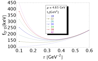
b)

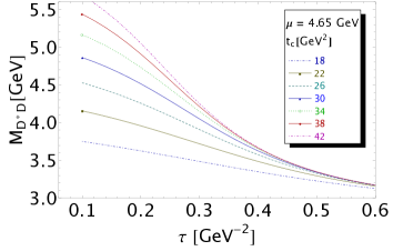
Figure 11: $f_{D^{*}D}$ and $M_{D^{*}D}$ as function of $\tau$ at NLO for different values of $t_{c}$, for $\mu$=4.65 GeV and for values of $\overline{m}_{c}(\overline{m}_{c})$ given in Table 2.

VI.1 $\tau$ and $t_{c}$-stabilities

We show in Fig. 11 the $\tau$-behaviour of the coupling and of the mass for different values of $t_{c}$ and fixing the value of the subtraction constant $\mu$ at 4.65 GeV (see next subsection) where a $\mu$ stability $(4.5\pm 0.5)$ GeV has been found in MOLE16 . From this figure, one can see that the coupling presents minimas in $\tau$ and the mass inflexion points.

– In a first step, we use the experimental mass $M_{Z_{c}}=3900$ MeV for extracting the value of the coupling $f_{D^{*}D}$ shown in Fig. 11a).

– In a 2nd step, we take the value of $\tau$ at the minimum of the coupling and use it for extracting the value of $M_{D^{*}D}$ from Fig. 11b).

– In a 3rd step, we take the common range of $t_{c}$ where both curves present stabilities in $\tau$. In the present case, this value ranges from $t_{c}=22$ GeV² (beginning of $\tau$-stability) to $t_{c}=38$ GeV² (beginning of $t_{c}$-stability) where the range is given in Table 4. For the mean $t_{c}=$ 30 GeV², it is : $\tau_{R}\simeq 0.38$(resp. 0.34) GeV^-2 for LO (resp. NLO) QCD expression.

– The errors given in Table 3 and the resulting values of $f_{D^{*}D}$ and $M_{D^{*}D}$ in Table 7 are the mean of the ones from the previous two extremal values of $t_{c}$.

VI.2 $\mu$-stability

For doing the analysis, we shall fix $t_{c}=30$ GeV² which is the mean of the two extremal values delimiting the stability region and take $M_{D^{*}D}=3900$ MeV for fixing the coupling. The analysis is shown in Fig. 12. One can see a $\mu$-stability for :

$$\mu=(4.65\pm 0.05)~{}{\rm GeV}~{},$$ (15)

at which we shall evaluate the results quoted in Table 3.

This value of $\mu$ from a more refined analysis is more precise than the conservative one $(4.5\pm 0.5)$ GeV quoted in MOLE16 . The results of the analysis are given in Tables 3 and  7.

One should note that the resummed QCD expression of the sum rule which obeys an “Homogeneous” Renormalization Group Equation (RGE) is obtained by putting $\mu^{2}=1/{\tau}$ in the QCD expression of the sum rule and where the parameters having anomalous dimension $\gamma$ run as $1/(\log{\tau\Lambda^{2}})^{\gamma/\beta}$ (see e.g. SNR ). We have often used this choice in the past (see SNB1 ; SNB2 ; SNB3 ) which corresponds here to the value:

$$\mu=1/\sqrt{\tau_{0}}\simeq 1.6~{}{\rm GeV},$$ (16)

at the $\tau$-minimum for $t_{c}$=30 GeV². However, this value is outside the $\mu$-stability region obtained previously and then does not correspond to the optimal choice of $\mu$. This is the reason why we have abandoned this choice $\mu^{2}=1/{\tau}$. This result does not support the argument of Ref. WANG1 based on the observation that, when the term of the type $(\alpha_{s}(\tau)/\alpha_{s}(\mu))^{{\gamma}/{\beta_{1}}}$ disappears for $\mu=1/\sqrt{\tau}$, one would obtain the best choice of $\mu$. Indeed, the PT series behaves obviously much better in the $\mu$-stability region where the value of $\mu$ is about 3 times higher at which the radiative corrections are more suppressed.

Moreover, the physical meaning of the relation between $\mu$ with the so-called bound energy or virtuality $\mu^{2}={M_{Z}^{2}-4M_{c}^{2}}$ used in his different papers (see e.g. WANG1 ; WANGMU ) remains unclear to us where $M_{c}$ is the PT constituent or pole charm quark mass taken by the author to be about 1.84 GeV which corresponds to $\mu\simeq$ 1.3 GeV.

Indeed, one may expect from this formula that the difference between the resonance and PT quark constituent masses has a non-perturbative origin which (a priori) has nothing to do with the scale $\mu$ where the PT series and the Wilson coefficients of the condensates are evaluated.

However, one may also consider $\mu$ as a scale separating the calculable PT Wilson coefficients and the NPT non-calculable condensates in the OPE SVZa though one has to bear in mind that the $d\leq 6$ condensates appearing in the present analysis are renormalization group invariant ($\mu$ independent like $m_{c}\langle\bar{q}q\rangle,~{}m^{2}_{c}\langle\bar{q}q\rangle^{2},$ ) or have a weak dependence on $\mu$ ($\langle\alpha_{s}G^{2}\rangle,\langle g\bar{q}Gq\rangle$) SNB1  (Part VII page 285) such that the truncation of the PT series does not affect much their values. This feature indicates that the separation of the condensates from the PT Wilson coefficients are not ambiguous while the size of the non-perturbative condensate is almost independent on the scale at which the PT series is truncated.

a)

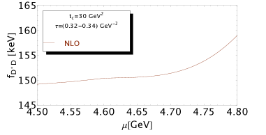
b)

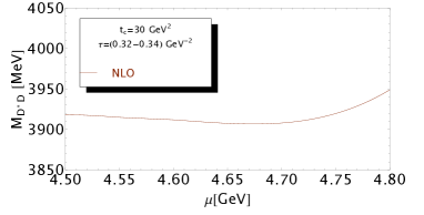
Figure 12: $f_{D^{*}D}$ and $M_{D^{*}D}$ as function of $\mu$ at NLO and for $t_{c}=30$ GeV².

VI.3 NLO and Truncation of the perturbative series

We have mentioned in previous works that the inclusion of the NLO perturbative corrections is important for justifying the choice of heavy quark mass definition used in the analysis where an ad hoc value of the $\overline{MS}$ running mass is frequently used in the literature while the spectral function has been evaluated using an on-shell renormalization where the pole (on-shell) quark mass naturally enters into the LO expression.

We show the analysis for the mass and coupling in Fig. 13 at fixed value of the continuum threshold $t_{c}$ and subtraction constant $\mu$, where one can find that the use of the pole mass at LO decreases by 30% at the minimum (resp. increases by 0.5% at the inflexion point) the value of the coupling (resp. mass) obtained using the $\overline{MS}$ running mass at LO while the NLO correction is relatively small within the $\overline{MS}$-scheme.

The smallness of radiative corrections for the ratio of moments demonstrates (a posteriori) why the use of the $\overline{MS}$ running mass at LO leads to a surprisingly good prediction for the mass.

a)

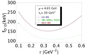
b)

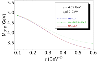
Figure 13: $f_{D^{*}D}$ and $M_{D^{*}D}$ as function of $\tau$ at LO and NLO for $t_{c}=30$ GeV² and $\mu=4.65$ GeV for different definitions of the charm quark mass. We use $m_{c}(pole)=1.5$ GeV and the running mass given in Table 2.

a)

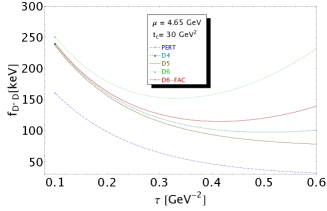
b)

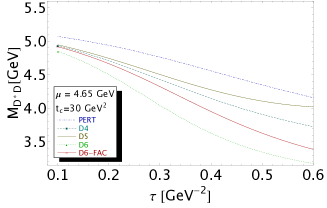
Figure 14: $f_{D^{*}D}$ and $M_{D^{*}D}$ as function of $\tau$ at NLO for $t_{c}=30$ GeV² and $\mu=4.65$ GeV and for different truncations of the OPE. $D4\equiv$ perturbative $\oplus$ dimension-4; $D5\equiv D4\oplus$ dimension-5; $D6\equiv D5\oplus$ dimension-6. The values of $\overline{m}_{c}(\overline{m}_{c})$ and the condensates are given in Table 2. FAC means that we use the vacuum saturation assumption for the estimate of the four-quark condensates.

Assuming that the PT series grow geometrically SZ ; CNZa ; CNZb ; ZAKa , one can deduce from the previous analysis an estimate of higher order PT contributions given in Table 3 which can be compared with the ones in  MOLE16 ; SU3 .

VI.4 QCD condensates and truncation of the OPE

We show in Fig. 14 the contributions of the QCD condensates for different truncations of the OPE. Fixing $\tau\approx 0.34$ GeV^-2 where the final value of the coupling presents $\tau$-stability and the mass inflexion points, one obtains for $t_{c}$=30 GeV² :

$$f_{D^{*}D} \simeq 56~{}{\rm keV}\big{[}1+0.98-0.13+0.86\big{]}$$

$$\simeq 151~{}{\rm keV},$$

$$M_{D^{*}D} \simeq 4683~{}{\rm MeV}\big{[}1-0.08+0.02-0.12\big{]}$$ (17)

$$\simeq 3864~{}{\rm MeV}~{}.$$

One can notice the important role of the dimension -4 and -6 condensates which are dominated by the chiral condensates $\langle\bar{q}q\rangle$ and $\rho\langle\bar{q}q\rangle^{2}$ in the extraction of the coupling and mass where their strengths are more pronounced for the coupling.

We estimate the sytematic errors due to the truncation of the OPE from the size of the dimension-6 condensate contributions rescaled by the factor $m^{2}_{c}\tau/3$ where 1/3 comes from the LSR exponential form of the sum rule. It can be compared with the contributions of the known $d=8$ $\langle\bar{q}q\rangle\langle\bar{q}Gq\rangle$ condensate obtained in MOLE16 ; SU3 but bearing in mind that this is only a part of the complete $d$=8 condensate ones where the validity of the vacuum saturation used for its estimate is questionable.

The quoted errors in Table 3 are the mean from the two extremal values of $t_{c}$ delimiting the $(\tau,t_{c})$ stability region. We expect that the systematics for the $m_{s}\not=0$ cases are similar as confirmed explicitly in Table 3.

VI.5 Vacuum saturation of the four-quark condensate

The four-quark condensates have been demonstrated to mix under renormalization SNTARRACH and SNB1  (Part VII page 285) at finite $N_{c}$ while its vacuum saturation estimate is only valid in the large $N_{c}$-limit. A such estimate from light mesons LNT ; LAUNERb , light baryons DOSCH ; JAMI2a ; JAMI2c and $\tau$-decays SNTAU has been shown to underestimate the actual value of the four-quark condensates by a factor 3-4 (see also the comments in Subsection IV.3). For completeness, we also show in Fig. 14 the effect of this estimate, where we see that the position of the minimum and inflexion point are shifted at $\tau\approx 0.4$ GeV^-2. At this value and for $t_{c}=30$ GeV², one obtains an effect of +38% for the coupling and –7% for the mass leading to :

$$f_{D^{*}D}|_{FAC}\simeq 115~{}{\rm keV},~{}~{}~{}~{}M_{D^{*}D}|_{FAC}\simeq 3951~{}{\rm MeV},$$ (18)

which can be compared with the one in Eq. 17.

VI.6 Results of the analysis

The sizes of the errors from different sources and the final results are collected inTables 3 and 7 :

$$f_{D^{*}D}=140(15)~{}{\rm keV},~{}~{}~{}~{}~{}M_{D^{*}D}=3912(61)\,{\rm MeV}~{}.$$ (19)

One can notice that the results are in perfect agreement with the previous ones in MOLE16 . The slight difference in the error calculation is due to the fact that, in Ref. MOLE16 , we have estimated the error by choosing $t_{c}=38$ GeV² but not considering the one due to $t_{c}=22$ GeV².

The result for the mass is in a very good agreement with the BELLE  BELLE1 and BESIII BES0 data $Z_{c}(3900)$ MeV which we shall discuss later on.

Observables	$\Delta t_{c}$	$\Delta\tau$	$\Delta\mu$	$\Delta\alpha_{s}$	$\Delta PT$	$\Delta m_{s}$	$\Delta m_{c}$	$\Delta\bar{\psi}\psi$	$\Delta\kappa$	$\Delta G^{2}$	$\Delta M_{0}^{2}$	$\Delta\bar{\psi}\psi^{2}$	$\Delta G^{3}$	$\Delta OPE$	$\Delta M_{G}$	$\Delta f_{G}$	$\Delta M_{(G)_{1}}$	Values
Coupling $f_{G}$ [keV]
Molecule $(c\bar{d})(\bar{c}u)$
$D^{*}D$	11.0	0.10	0.50	2.10	0.03	–	1.25	1.90	–	0.0	1.15	5.60	0.0	6.20	3.12	–	–	140(15)
$D^{*}_{0}D_{1}$	9.80	0.20	0.14	0.80	17.0	–	0.70	4.30	–	0.14	1.60	7.60	0.06	7.30	2.08	–	–	96(23)
Tetraquark $(\bar{c}\bar{d})(cu)$
$A_{cd}$	12.6	0.10	0.60	2.90	0.47	–	1.60	2.80	–	0.0	1.80	6.60	0.0	8.16	3.11	–	–	173(17)
Molecule $(c\bar{s})(\bar{c}u)$
$D^{*}_{s}D$	12.4	0.10	0.50	2.40	0.07	0.0	2.0	1.90	3.20	0.0	0.90	4.30	0.0	4.80	1.93	–	–	130(15)
$D^{*}D_{s}$	12.2	0.10	0.50	2.40	0.11	0.07	1.40	1.70	3.20	0.02	1.30	4.40	0.03	7.0	2.19	–	–	133(16)
$D^{*}_{s0}D_{1}$	9.0	0.20	0.45	0.53	18.0	0.48	0.85	4.10	1.12	0.36	1.65	6.60	0.33	6.90	1.97	–	–	86(23)
$D^{*}_{0}D_{s1}$	8.60	0.20	0.15	0.86	17.5	0.20	0.75	3.60	1.60	0.02	1.80	6.50	0.07	6.90	1.95	–	–	89(22)
Tetraquark $(\bar{c}\bar{s})(cu)$
$A_{cs}$	13.2	0.12	0.60	2.80	0.01	0.20	1.60	1.90	3.70	0.0	2.0	5.40	0.0	6.70	2.34	–	–	148(17)
Molecule $(c\bar{s})(\bar{c}s)$
$D^{*}_{s}D_{s}$	9.60	0.11	0.40	2.40	1.40	0.10	1.30	2.0	5.90	0.0	1.10	3.50	0.05	2.40	3.35	–	–	114(13)
$D^{*}_{s0}D_{s1}$	9.60	0.20	0.13	0.80	5.90	0.41	0.75	4.35	1.73	0.05	1.58	5.50	0.08	3.50	2.31	–	–	79(14)
Tetraquark $(\bar{c}\bar{s})(cs)$
$A_{css}$	10.9	0.14	0.50	2.80	0.90	0.25	1.40	2.10	6.90	0.0	2.0	4.40	0.10	5.20	2.40	–	–	114(15)
Mass $M_{G}$ [MeV]
Molecule $(c\bar{d})(\bar{c}u)$
$D^{*}D$	15.0	40.0	2.0	6.30	0.0	–	2.80	13.5	–	0.0	5.30	11.0	0.0	39.0	–	–	–	3912(61)
$D^{*}_{0}D_{1}$	1.60	105	4.50	9.50	2.50	–	7.10	50.0	–	1.80	12.0	40.0	0.30	39.5	–	–	–	4023(130)
Tetraquark $(\bar{c}\bar{d})(cu)$
$A_{cd}$	8.30	38.0	1.90	7.50	1.90	–	2.90	10.0	–	0.06	4.90	7.10	0.0	39.5	–	–	–	3889(58)
Molecule $(c\bar{s})(\bar{c}u)$
$D^{*}_{s}D$	5.70	37.8	2.50	7.50	0.23	2.50	3.0	8.0	15.0	0.0	7.0	10.0	0.0	25.4	–	–	–	3986(51)
$D^{*}D_{s}$	1.50	37.6	2.0	7.0	0.03	2.70	2.30	8.80	17.0	0.06	10.0	6.20	0.18	33.8	–	–	–	3979(56)
$D^{*}_{s0}D_{1}$	13.1	105	4.25	6.25	1.30	3.75	6.50	20.0	44.0	0.20	18.0	20.9	0.23	57.5	–	–	–	4064(133)
$D^{*}_{0}D_{s1}$	18.8	102	4.0	8.80	0.28	2.80	5.30	30.3	51.2	0.06	12.6	19.3	0.16	52.8	–	–	–	4070(133)
tetraquark $(\bar{c}\bar{s})(cu)$
$A_{cs}$	8.50	38.8	2.0	6.90	0.03	2.20	2.40	7.60	16.0	0.07	7.50	6.70	0.0	33.5	–	–	–	3950(56)
Molecule $(c\bar{s})(\bar{c}s)$
$D^{*}_{s}D_{s}$	0.30	42.5	2.40	6.0	12.0	6.20	2.10	6.70	15.3	0.05	9.10	13.8	0.05	25.7	–	–	–	4091(57)
$D^{*}_{s0}D_{s1}$	0.10	108	2.75	4.30	0.05	5.0	10.3	15.0	30.5	0.25	15.0	30.3	0.38	50.1	–	–	–	4198(129)
Tetraquark $(\bar{c}\bar{s})(cs)$
$A_{css}$	1.60	44.0	15.0	15.0	0.06	16.0	13.0	23.0	16.0	0.15	12.3	17.0	0.08	43.7	–	–	–	4014(77)

Table 3: Sources of errors and predictions from LSR at NLO for the couplings and masses of the molecules and tetraquark ground states. The errors from the QCD input parameters are from Table 2. We take $|\Delta\tau|=0.01$ GeV^-2 and $\Delta\mu=0.05$ GeV. The quoted errors are the mean from the two extremal values of $t_{c}$ delimiting the stability region quoted in Table 4.

States	($1^{+}$) ground states
Parameters	$D^{*}D$	$D^{*}_{s}D$	$D^{*}D_{s}$	$D^{*}_{s}D_{s}$	$D^{*}_{0}D_{1}$	$D^{*}_{s0}D_{1}$	$D^{*}_{0}D_{s1}$	$D^{*}_{s0}D_{s1}$	$A_{cd}$	$A_{cs}$	$~{}A_{css}$
$t_{c}$ [GeV2]	22 – 38	22 – 38	22 – 38	24 – 40	28 – 40	28 – 44	28 – 44	28 – 44	22 – 38	22 – 8	24 – 40
$\tau$ [GeV]${}^{-2}10^{2}$	23 ; 35	22 ; 36	24 ; 38	24 ; 36	21 ; 30	20 ; 30	23 ; 31	20 ; 30	25 ; 37	25 ; 38	27 ; 38

Table 4: Values of the set of the LSR parameters $(t_{c},\tau)$ at the optimization region for the PT series up to NLO and for the OPE truncated at the dimension-six condensates and for $\mu=4.65$ GeV.

VII Revisiting $f_{D^{*}_{0}D_{1},A_{cd}}$ and $M_{D^{*}_{0}D_{1},A_{cd}}$

Here, we also revisit the estimate of the $D^{*}_{0}D_{1},A_{cd}$ masses and couplings done in MOLE16 . We repeat exactly the same procedure as in the previous section.

VII.1 $f_{D^{*}_{0}D_{1}}$ and $M_{D^{*}_{0}D_{1}}$

The $\tau$ and $t_{c}$-behaviours of the coupling and mass are similar to the previous case and will not be shown here. The $\tau$-stability region ranges from $\tau=0.21$ GeV^-2 for $t_{c}=$ 28 GeV² (beginning of $\tau$-stability) to 0.30 GeV^-2 for $t_{c}$= 40 GeV² (beginning of $t_{c}$-stability). One can notice that the $\tau$-stability starts at a larger value of $t_{c}$ than the one $t_{c}=22$ GeV² for the case of $D^{*}D$ which will imply a larger value of $M_{D^{*}_{0}D_{1}}$ than of $M_{D^{*}D}$.

The $\mu$-stability is shown in Fig. 15 where the optimal value is the same as in Eq. 15. The result :

$$f_{D^{*}_{0}D_{1}}=96(23)~{}{\rm keV},~{}~{}~{}~{}M_{D^{*}_{0}D_{1}}=4023(130)~{}{\rm MeV},$$ (20)

differs with the one given in MOLE16 ; SU3 (see Table 7) originated from the unprecise value of the $\tau$ used there for extracting the optimal value which affect in a sensible way the value of the mass in this channel.

a)

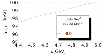
b)

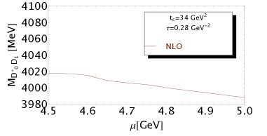
Figure 15: $f_{D^{*}_{0}D_{1}}$ and $M_{D^{*}_{0}D_{1}}$ as function of $\mu$ at NLO and for $t_{c}=30$ GeV².

VII.2 $f_{A_{cd}}$ and $M_{A_{cd}}$

The $\tau$ and $t_{c}$-behaviours of the $A_{cd}$-mass and coupling are similar to the one in Fig 11. The $\tau$-stability starts for $t_{c}$=22 GeV² at $\tau=0.25$ GeV^-2 while the $t_{c}$-stability starts at $t_{c}=$ 38 GeV² where $\tau=0.36$ GeV^-2.

The $\mu$-behaviours are the same as the ones of $D^{*}_{0}D_{1}$ where the $\mu$-stability is also at 4.65 GeV as in Eq. 15.

The estimates of the errors and the results for the coupling and mass :

$$f_{A_{cd}}=173(17)~{}{\rm keV}~{}~{}~{}~{}~{}~{}~{}~{}M_{A_{cd}}=3889(58)~{}{\rm MeV}$$ (21)

are collected in Tables 3 and 7. The mass value is in good agreement with the one 3888(130) MeV obtained in Ref. MOLE16 but with a smaller error due to a better localisation of the $\tau$ and $\mu$ stability points. The $A_{cd}$ mass also coincides with the observed $Z_{c}(3900)$. The different sets of $(t_{c},\tau)$ used to get the previous optimal results are summarized in Table 4.

VIII The $(1^{+})$ $(c\bar{s})(\bar{c}u)$ and $(\bar{c}\bar{s})(cu)$states

VIII.1 New estimate of $f_{D^{*}_{s}D}$ and $M_{D^{*}_{s}D}$

In this section, we present a new estimate of the $D^{*}_{s}D$ molecule mass and coupling.

a)

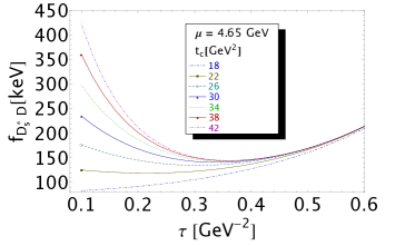
b)

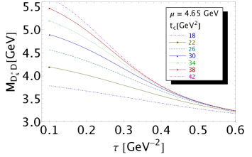
Figure 16: $f_{D^{*}_{s}D}$ and $M_{D^{*}_{s}D}$ as function of $\tau$ at NLO for different values of $t_{c}$, for $\mu$=4.65 GeV and for values of $\overline{m}_{c}(\overline{m}_{c})$ given in Table 2.

a)

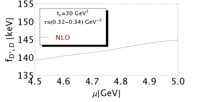
b)

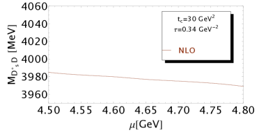
Figure 17: $f_{D^{*}_{s}D}$ and $M_{D^{*}_{s}D}$ as function of $\mu$ at NLO and for $t_{c}=30$ GeV².

a)

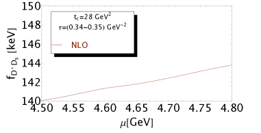
b)

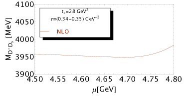
Figure 18: $f_{D^{*}D_{s}}$ and $M_{D^{*}D_{s}}$ as function of $\mu$ at NLO and for $t_{c}=28$ GeV².

The $\tau$ and $t_{c}$-behaviours of the coupling and mass are also similar to the previous cases as shown in Fig. 16.

The $\tau$-stability region ranges from $\tau=0.22$ GeV^-2 for $t_{c}=$ 22 GeV² (beginning of $\tau$-stability) until 0.36 GeV^-2 for 38 GeV² (beginning of $t_{c}$-stability).

The $\mu$-stability is shown in Fig. 17 where the optimal value is the same as in Eq. 15.

The sources of the errors and the results are quoted in Table 3 and 7 . One can notice that the values of the $\tau,~{}t_{c}$ and $\mu$-stabilities are about the same as in the case of $D^{*}D$ indicating a good $SU(3)$ symmetry for the sum rule parameters. The obtained values quoted in Tables 3 and 7 :

$$f_{D^{*}_{s}D}=130(15)~{}{\rm keV},~{}~{}~{}~{}M_{D^{*}_{s}D}=3986(51)~{}{\rm MeV}$$ (22)

also indicate small $SU(3)$ breakings of chiral symmetry which is about $-7.1\%$ for the coupling and $+1.9\%$ for the mass.

VIII.2 New estimate of $f_{D^{*}D_{s}}$ and $M_{D^{*}D_{s}}$

A similar analysis is done for extracting $f_{D^{*}D_{s}}$ and $M_{D^{*}D_{s}}$. The $\tau$ and $t_{c}$ behaviours of the results are similar to the previous ones. The $\mu$-behaviour is is shown in Fig. 18. We obtain :

$$f_{D^{*}D_{s}}=133(16)~{}{\rm keV},~{}~{}~{}~{}M_{D^{*}D_{s}}=3979(56)\,{\rm MeV},$$ (23)

where the values of the parameters are about the same as the ones of $D^{*}_{s}D$ as intuitively expected. They are quoted in Tables 3 and 7.

VIII.3 The $D^{*}_{s0}D_{1}$ and $D^{*}_{0}D_{s1}$ molecules

Similar analysis leads to (see Tables 3 and 7) :

$$f_{D^{*}_{s0}D_{1}}=86(23)~{}{\rm keV},~{}M_{D^{*}_{s0}D_{1}}=4064(133)\,{\rm MeV},$$

$$f_{D^{*}_{0}D_{s1}}=89(23)~{}{\rm keV},~{}M_{D^{*}_{0}D_{s1}}=4070(133)\,{\rm MeV},$$ (24)

where one can notice that the two molecule states are almost degenerated and have the same couplings to the currents.

VIII.4 The $A_{cs}$ tetraquark

We pursue the previous analysis for the $A_{cs}$ tetraquark. The behaviours of the different curves are similar to the previous ones and will not be shown. The result quoted in Tables 3 and 7 is:

$$f_{A_{cs}}=148(17)~{}{\rm keV},~{}~{}~{}~{}~{}M_{A_{cs}}=3950(56)\,{\rm MeV}~{},$$ (25)

where one can notice that it is almost degenerated to the $D^{*}D_{s}$ and $D^{*}_{s}D$ and has almost the same couplings.

IX The $(1^{+})$ $(c\bar{s})(\bar{c}s)$ and $(\bar{c}\bar{s})(cs)$ states

In this section, we revisit and improve our previous estimate of the masses and couplings of these above-mentioned states and give a new estimate of the $D^{*}_{s}D_{s}$ radial excitation mass and coupling.

IX.1 The ${D^{*}_{s}D_{s}}$ molecule

The analysis of the $\tau$ and $t_{c}$ behaviours is shown in Fig. 19. The $\mu$-behaviour is shown in Fig. 20. These behaviours are similar to the previous ones. The $(\tau,t_{c})$ stabilities are obtained for $t_{c}$ inside the range 24 to 40 GeV². We deduce (see Tables 3 and 7) :

$$f_{D^{*}_{s}D_{s}}=114(13)~{}{\rm keV},~{}~{}~{}M_{D^{*}_{s}D_{s}}=4091(57)\,{\rm MeV},$$ (26)

One can notice the (almost) similar effect of $SU(3)$ breakings than in the previous cases. The mass increases by 105 MeV compared to the one of the $D^{*}_{s}D$ state which is about the one 74 MeV from $D^{*}D$ to $D^{*}_{s}D$.

a)

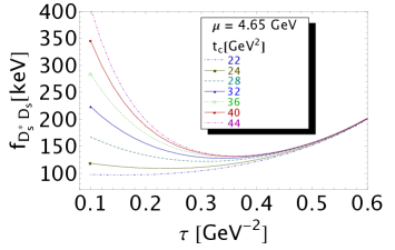
b)

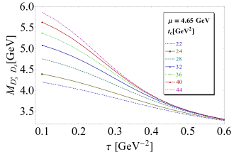
Figure 19: $f_{D^{*}_{s}D_{s}}$ and $M_{D^{*}_{s}D_{s}}$ as function of $\tau$ at NLO for different values of $t_{c}$, for $\mu$=4.65 GeV and for values of $\overline{m}_{c}(\overline{m}_{c})$ given in Table 2.

a)

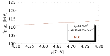
b)

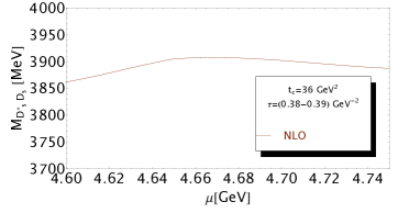
Figure 20: $f_{D^{*}_{s}D_{s}}$ and $M_{D^{*}_{s}D_{s}}$ as function of $\mu$ at NLO and for $t_{c}=36$ GeV².

IX.2 The $D^{*}_{s0}D_{s1}$ molecule and $A_{css}$ tetraquark

In this section, we revise and check the results obtained in SU3 . The behaviours of the $\tau,t_{c}$ and $\mu$-behaviours of the masses and couplings are similar to the previous cases and will not be shown.

For the $D^{*}_{s0}D_{s1}$ molecule, the set of $(\tau,t_{c})$-stabilities are obtained from (0.20,28) to (0.30,44) in units of (GeV^-2, GeV²), where one notice the sensitivity of the results in the change of $\tau$ which is quantified by the large error induced by the variation of $\tau$ as shown in Table 3. One obtains from Tables 3 and 7 :

$$f_{D^{*}_{s0}D_{s1}}=79(14)~{}{\rm keV},~{}~{}~{}M_{D^{*}_{s0}D_{s1}}=4198(129)\,{\rm MeV},$$ (27)

which agree within the errors with the previous results in SU3 .

For the $A_{css}$ tetraquark, $\tau$-stability at 0.27 GeV^-2 starts for $t_{c}=24$ GeV² while the $t_{c}$-stability for $\tau=0.38$ GeV^-2 starts for $t_{c}=40$ GeV². These values are about the same as the ones for $A_{cd}$ and $A_{cs}$ indicating like in the case of molecule states a good $SU(3)$ symmetry for the values of the LSR parameters. The optimal results are given in Tables  3 and  7 which read:

$$f_{A_{css}}=114(16)~{}{\rm keV}~{},~{}~{}~{}~{}~{}M_{A_{css}}=4014(86)\,{\rm MeV}~{}.$$ (28)

Compared to the previous non-strange case where the molecule $D^{*}D$ is quasi-degenerated with the tetraquark $A_{cd}$, which leads us to conclude that the observed state is a tetramole ${\cal T}_{c}$, in this channel, we find the tetraquark $A_{css}$ is almost degenerated (within the errors) with the molecule $D^{*}_{s}D_{s}$ and has the same couplings implying that it can also be a tetramole ${\cal T}_{css}$ state with a coupling and mass:

$$f_{{\cal T}_{css}}=114(10)~{}{\rm keV}~{},~{}~{}~{}~{}~{}M_{{\cal T}_{css}}=4064(46)\,{\rm MeV}~{}.$$ (29)

The $D^{*}_{s0}D_{s1}$ molecule is about 100 MeV slightly higher but has a weaker coupling to the corresponding current.

X Two-meson scattering states 

To study this contribution, we take the example of the $D^{*}D$ molecule .

We saturate the RHS of Fig. 9 by the two non-resonant (scattering) states $D^{*}$ and $D$ which we shall compare with the one due to the molecule $D^{*}D$ (LHS) appropriately matched with the $k^{2}$-factor.

Then, one obtains the two-resonance scattering LSR moment :

$${\cal L}^{c}_{0}({D^{*}\oplus D}) \equiv 2\left(\frac{k}{4\pi}\right)^{2}f^{2}_{D^{*}}\left(\frac{f_{D}}{m_{c}}\right)^{2}{\cal I}(t,M_{D}^{2},M_{D^{*}}^{2})$$ (30)

$$\simeq 1.16\times 10^{-6}{\rm GeV}^{10},$$

where ${\cal I}(t,M_{D}^{2},M_{D^{*}}^{2})$ is the integral (see Eq. III.3):

$${\cal I}\equiv\int_{(M_{D}+M_{D^{*}})^{2}}^{t_{c}}dt\,t^{2}\,{\rm e}^{-t\tau}\int_{{M_{D}}^{2}}^{(\sqrt{t}-M_{D^{*}})^{2}}dt_{1}\hskip 17.07182pt\int_{M_{D^{*}}^{2}}^{(\sqrt{t}-\sqrt{t_{1}})^{2}}dt_{2}\,\lambda^{3/2}\left(\frac{M_{D}^{2}}{t},\frac{M_{D^{*}}^{2}}{t}\right),$$ (31)

to be compared with the molecule sum rule result :

$${\cal L}_{0}^{c}({D^{*}D})\equiv f^{2}_{D^{*}D}M^{8}_{D^{*}D}\,{\rm e}^{-\tau_{R}M^{2}_{D^{*}D}}\simeq 1.09\times 10^{-5}{\rm GeV}^{10},$$ (32)

which we have evaluated at the stability point $\tau_{R}\simeq 0.3$ GeV^-2. We have used the previous values of the molecule parameters $f_{D^{*}D}$=140 keV and $M_{D^{*}D}$=3.91 GeV given in Table 3 and the average values of $f_{D}=204(6)$ MeV and $f_{D^{*}}=250(8)$ MeV from SNFB15 ; SNFB15 ; SNB2 . We have neglected the equal and small contributions to the two sum rules from the QCD continuum above the continuum threshold taken to be : $t_{c}\approx 30$ GeV² which is the mean of the two extremal values delimiting the stability region. These results indicate that :

– For finite $N_{c}$, the non-resonant contribution is about one order of magnitude smaller than the one of the resonance molecule (a similar conclusion using an alternative approach has been reached in WANG1 ) and disprove the claim of Ref. LUCHA based on large $N_{c}$ once an appropriate matching of the two correlators via the $k^{2}$ factor is done.

– A posteriori, the existence of the stability region or “sum rule window” in the LSR analysis where one can extract the (postulated) resonance mass and coupling using the spectral function parametrization within the duality ansatz “one resonance” + QCD continuum is a strong indication of the duality between the QCD-OPE and the phenomenological side of the sum rule, where the resonace contribution is dominant over the one of the non-resonant states. This fact does not also support the claim of Ref. LUCHA .

XI Radial excitations

We present in this section a new estimate of the couplings and masses of the first radial excitations using the lowest moments ${\cal L}^{c}_{0}$ and ${\cal R}_{0}^{c}$ . In so doing, we use a “two resonance” parametrization of the spectral function.

XI.1 The $(D^{*}D)_{1}$ first radial excitation

We insert the previously obtained values of the lowest ground state $D^{*}D$ mass and coupling and study the $\tau$ - and $t_{c}$-stability of the sum rules by fixing the subtraction constant $\mu$ as in Eq. 15. The analysis is shown in Fig. 21 where the stability region is delimited by $t_{c}$ = 39 and 50 GeV² to which corresponds respectively the $\tau$-stability of (0.14–0.18) and (0.28–0.29) GeV^-2. The results :

$$f_{(D^{*}D)_{1}}=197(25)~{}{\rm keV},~{}~{}M_{(D^{*}D)_{1}}=5709(70)~{}{\rm MeV}$$ (33)

are quoted in Table 5. The set of $(t_{c},\tau)$ is compiled in Table 6.

a)

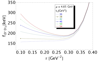
b)

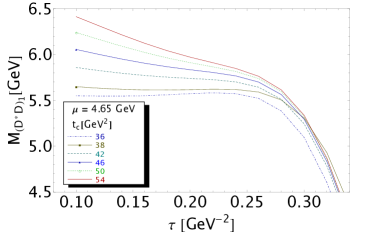
Figure 21: $f_{(D^{*}D)_{1}}$ and $M_{(D^{*}D)_{1}}$ as function of $\tau$ at NLO for different values of $t_{c}$, for $\mu$=4.65 GeV and for values of $\overline{m}_{c}(\overline{m}_{c})$ given in Table 2.

One can notice that the mass value is roughly about the (expected) one of $\sqrt{t_{c}}\simeq(4.7-6.2)$ GeV inside the stability region where the lowest ground state mass has been extracted.

Observables	$\Delta t_{c}$	$\Delta\tau$	$\Delta\mu$	$\Delta\alpha_{s}$	$\Delta PT$	$\Delta m_{s}$	$\Delta m_{c}$	$\Delta\bar{\psi}\psi$	$\Delta\kappa$	$\Delta G^{2}$	$\Delta M_{0}^{2}$	$\Delta\bar{\psi}\psi^{2}$	$\Delta G^{3}$	$\Delta OPE$	$\Delta M_{G}$	$\Delta f_{G}$	$\Delta M_{(G)_{1}}$	Values
Coupling $f_{G}$ [keV]
$(D^{*}D)_{0}$	21	0.7	2.9	11	6.2	–	8.5	8.2	–	0.09	4.5	26.8	0.10	19	14.5	34	–	46(56)
$(D^{*}D)_{1}$	10.0	0.18	1.35	8.5	0.60	–	5.60	9.30	–	0.06	3.70	7.40	0.07	3.71	1.80	15.1	10.1	197(25)
$(D^{*}_{0}D_{1})_{1}$	5.2	0.5	0.4	4.3	9.3	–	4.7	19.25	–	0.10	6.30	10.5	0.28	9.10	0.45	16.5	26.0	238(41)
$(A_{cd})_{1}$	18.9	0.12	2.29	11.8	9.60	–	7.31	9.49	–	0.04	6.04	7.43	0.15	6.41	4.05	15.1	17.2	272(38)
$(D^{*}_{s}D)_{1}$	9.0	0.20	1.50	8.8	0.20	0.95	4.90	8.65	10.5	0.06	2.20	6.9	0.08	6.1	1.75	16.8	8.70	199(29)
$(D^{*}_{s}D_{s})_{1}$	6.5	0.60	1.80	9.5	4.9	1.5	4.6	11.7	13.0	0.18	4.80	10.0	0.20	12.4	7.30	16.2	27.1	197(43)
Mass $M_{G}$ [MeV]
$(D^{*}D)_{1}$	30.0	38.9	11.8	5.0	0.02	–	16.5	10.0	–	1.10	29.5	6.0	1.15	23.0	18.0	12	–	5709(70)
$(D^{*}_{0}D_{1})_{1}$	83.0	2.5	0.4	10	14	–	11.8	55.2	–	0.2	34	74.6	0.7	50.6	20.8	55	–	6375(152)
$(A_{cd})_{1}$	59.0	15.2	9.46	6.54	3.81	–	19.1	26.4	–	0.15	22.5	4.96	0.80	14.3	20.7	26.5	–	5717(82)
$(D^{*}_{s}D)_{1}$	2.0	30.0	16.5	7.5	0.02	2.0	18.5	13.0	6.0	0.85	20.5	4.0	1.40	10.0	19.0	10	–	5725(52)
$(D^{*}_{s}D_{s})_{1}$	42.0	49.0	39.5	42.5	1.05	4.5	20.5	38.5	45.5	1.0	35.0	58.0	3.0	40.8	25.5	69.0	–	5786(152)

Table 5: Sources of errors and predictions from LSR at NLO and for the decay constants and masses of the molecules and tetraquark radial excitation states. The errors from the QCD input parameters are from Table 2. We take $|\Delta\tau|=0.01$ GeV^-2 and $\Delta\mu=0.05$ GeV. The quoted errors have been estimated fixing $t_{c}$ at the mean of the two extremal values delimiting the stability region quoted in Table 6. We notice that the relative large values of some individual errors in the case of ${D^{*}_{s}D_{s}}$ and $(D^{*}_{0}D_{1})_{1}$ are mainly induced by the shift of the position of the minima compared to the one of the central values.

States	($1^{+}$) radial excitations
Parameters	$(D^{*}D)_{0}$	$(D^{*}D)_{1}$	$(D^{*}_{0}D_{1})_{1}$	$(A_{c})_{1}$	$(D^{*}_{s}D)_{1}$	$(D^{*}_{s}D_{s})_{1}$
$t_{c}$ [GeV2]	27 – 46	39 – 50	48 – 56	39 – 50	40 – 50	42 – 52
$\tau$ [GeV]${}^{-2}10^{2}$	30 ; 34	13 ; 26	15, 24 ; 20, 25	7, 26; 29, 27	9 ; 27	21 ; 29

Table 6: Values of the set of the LSR parameters $(t_{c},\tau)$ at the optimization region for the PT series up to NLO and for the OPE truncated at the dimension-six condensates and for $\mu=4.65$ GeV. The first set for $(D^{*}_{0}D_{1})_{1}$ and $(A_{c})_{1}$ correspond repsectively to the mass and coupling.

XI.2 The $(D^{*}_{0}D_{1})_{1}$ radial excitation

We show the analysis in Fig. 22. The curves have similar behaviour as in the case of $(D^{*}D)_{1}$ but the stabilities are reached for higher values of $t_{c}$ which imply a higher value of the $(D^{*}_{0}D_{1})_{1}$ radial excitation mass. The results are quoted in Table 5 and the set of $(t_{c},\tau)$ is compiled in Table 6.

a)

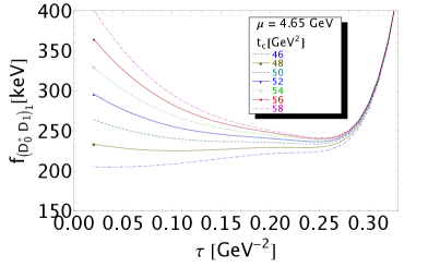
b)

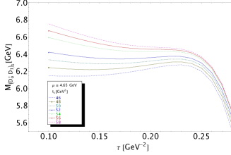
Figure 22: $f_{(D^{*}_{0}D_{1})_{1}}$ and $M_{(D^{*}_{0}D_{1})_{1}}$ as function of $\tau$ at NLO for different values of $t_{c}$ and for $\mu$=4.65 GeV.

XI.3 The $(A_{cd})_{1}$ radial excitation

The behaviours of the coupling and mass versus $\tau$ and $t_{c}$ are similar to the case of the one of $(D^{*}D)_{1}$ and will not be repeated here. The results are quoted in Table 5.

XI.4 The $(D^{*}_{s}D)_{1}$ radial excitation

We estimate the mass and coupling of the $(D^{*}_{s}D)_{1}$ radial excitation like in the case of $(D^{*}D)_{1}$. The analysis is similar and the curves have the same behaviours. The set of LSR parameters used to get the results are quoted in Table 6. We obtain the results quoted in Tables 5 :

$$f_{(D^{*}_{s}D)_{1}}=199(29)~{}{\rm keV},~{}~{}M_{(D^{*}_{s}D)_{1}}=5725(52)~{}{\rm MeV}~{},$$ (34)

where they are also quite high compared to the ones of ordinary mesons.

XI.5 The first radial excitation $(D^{*}_{s}D_{s})_{1}$

In this subsection, we study the first radial excitation $(D^{*}_{s}D_{s})_{1}$. The $\tau$ and $t_{c}$ behaviours of its mass and coupling are shown in Fig. 23 for $\mu=4.65$ GeV. The $\tau$ and $t_{c}$-stabilities are reached for the set $(\tau,t_{c})$ =(0.28,42) to (0.30,54) in units of (GeV^-2, GeV²). We deduce (see Table 5) :

$$f_{(D^{*}_{s}D_{s})_{1}}=197(43)~{}{\rm keV},~{}~{}M_{(D^{*}_{s}D_{s})_{1}}=5786(152)\,{\rm MeV}.$$ (35)

One can notice that the coupling of the 1st radial excitation is similar to the previous radial excited states which are relatively large compared to the ones of lowest ground states. This feature differs from the case of ordinary mesons built from bilinear currents. The mass is also found to be relatively high.

a)

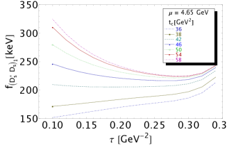
b)

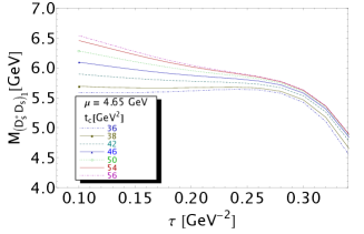
Figure 23: $f_{(D^{*}_{s}D_{s})_{1}}$ and $M_{(D^{*}_{s}D_{s})_{1}}$ as function of $\tau$ at NLO for different values of $t_{c}$ and for $\mu$=4.65 GeV.

XI.6 Comments on the radial excitations

We have shown previously that the couplings of the excited states to the corresponding currents are as large as the one of the ground states (see Table 5) which is a new feature compared to the case of ordinary hadrons.

We have also shown that the mass-splittings between the first radial excitation and the lowest ground state are (see Table 5) :

$$M_{(G)_{1}}-M_{G}\simeq(1.70\sim 2.35)~{}{\rm GeV},$$ (36)

which is much bigger than the one $(500\sim 600)$ MeV for ordinary mesons but comparable with the one obtained for the $DK$ state in DK . The authors in Ref. WANGMU have also noticed a such anomalously large value of the mass of the radial excitation $M_{R1}\approx\sqrt{t_{c}}\geq 4.5$ GeV in the analysis of the $Z_{c}(4020,4025)$. Then, they have concluded that the $Z_{c}(4020,4025)$ cannot be a tetraquark state as the value of $t_{c}$ used to extract these masses is much larger than the one expected from the empirical relation :

$$\sqrt{t_{c}}\approx M_{Z_{c}}+0.5~{}{\rm GeV},$$ (37)

where the value 0.5 GeV has been inspired from ordinary mesons and from the results of LEBED .

From our result, one can already conclude that the $Z_{c}(4020)$ to $Z_{c}(4430)$ are too low to be the radial excitations of the $Z_{c}(3900)$ unless they couple weakly to the interpolating current such that their effect is tiny in the LSR analysis.

XI.7 Can there be a weakly coupled radial excitation

If one literally extrapolates the phenomenological observation from ordinary hadrons, one would expect a radial excitation with a mass:

$$M_{(D^{*}D)_{0}}\approx M_{D^{*}D}+0.5~{}{\rm GeV}\simeq 4.4~{}{\rm GeV}~{},$$ (38)

which is relatively low compared to the previous prediction in Eq. 33 but seems to fit the $Z_{c}(4430)$. To understand why it can have been eventually missed in the previous analysis, we shall determine the $Z_{c}(4430)$ coupling to the current and use as input the experimental mass value .

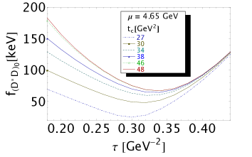
Figure 24: The coupling $f_{(D^{*}D)_{0}}$ of the $Z_{c}(4430)$ at NLO as a function of $\tau$ for different values of $t_{c}$ and for $\mu=4.65$ GeV.

In so doing, we reconsider the ${\cal L}^{c}_{0}$ moment. We use a two-resonance parametrization of the spectral function and introduce as inputs the previous values of the $D^{*}D$ molecule mass and coupling. We use the experimental mass of the $Z_{c}(4430)$. We include the high-mass $(D^{*}D)_{1}$ radial excitation obtained previously into the QCD continuum contribution.

We show the $\tau$-behaviour of the coupling for different $t_{c}$-values and for fixed $\mu=4.65$ GeV in Fig. 24. At the $(\tau,t_{c})$ stability regions $(0.30,27)$ to $(0.34,46)$ (GeV^-2, GeV²), we deduce :

$$f_{(D^{*}D)_{0}}=46(56)~{}{\rm keV}~{},$$ (39)

where the different sources of the errors are given in Table 5. The coupling is indeed relatively small compared to that of $f_{D^{*}D}=140$ keV. It can even be consistent with zero due to the large errors mainly induced by the coupling of the ground state and of the dimension-6 condensates. This result may support an eventual radial excitation interpretation of the $Z(4340)$ which couples very weakly to the current and having a mass much lower than the strongly coupled [$f_{(D^{*}D)_{1}}=197$ MeV] radial excitation with a mass 5709 MeV (see Table 5). This weak coupling disagrees with the one obtained in Ref WANGRAD and may originate from the fact that the latter analysis has been done at a smaller value of $t_{c}$ and at the scale $\mu=1.5$ GeV which is too low compared to the optimal choice obtained in the present work. However, as we have already mentioned in Subsection VI.2, we do not find any convincing theoretical basis for justifying this low choice of $\mu$. We expect that similar results can be obtained in some other channels.

XII Versus our previous results

States	Couplings			Masses
	Ref. MOLE16	Ref. SU3	New	Ref. MOLE16	Ref. SU3	New
Molecule $(\bar{c}d)(c\bar{u})$
$D^{*}D$	154(7)	–	140(15)	3901(62)	–	3912(61)
$D^{*}_{0}D_{1}$	96(15)	–	96(23)	4394(164)	3854(182)	4023(130)
Tetraquark $(\bar{c}\bar{d})(cu)$
$A_{cd}$	176(30)	–	173(17)	3890(130)	–	3889(42)
Molecule $(c\bar{s})(\bar{c}u)$
$D^{*}_{s}D$	–	–	130(15)	–	–	3986(51)
$D^{*}D_{s}$	–	–	133(16)	–	-	3979(56)
$D^{*}_{s0}D_{1}$	–	–	86(23)	–	-	4064(133)
$D^{*}_{0}D_{s1}$	–	–	89(22)	–	-	4070(133)
Tetraquark $(\bar{c}\bar{s})(cu)$
$A_{cs}$	–	–	148(17)	–	–	3950(56)
Molecule $(\bar{c}s)(c\bar{s})$
$D^{*}_{s}D_{s}$	–	114(13)	–	–	3901(62)	4091(57)
$D^{*}_{s0}D_{s1}$	–	79(14)	70(16)	–	4269(205)	4198(129)
$A_{css}$	–	114(16)	131(14)	–	4209(112)	4014(86)

Table 7: Summary of the couplings and masses predictions of the lowest ground states and comparison with our previous results in Refs. MOLE16 ; SU3 .

We compare our results with our previous ones from Refs. MOLE16 ; SU3 in Table 7. Notice that in  SU3 , the double ratio of moments has been also used to extract directly the $SU(3)$ breaking contributions to the masses and couplings. One can notice a good agreement between the different results. The exception is the central value of $M_{D^{*}_{0}D_{1}}$ which slightly moves in the 3 papers though the results are in agreement within the errors. This is due to the difficult localization of the inflexion point which we have identified in the present work with the minimum of the coupling like in some other channels.

XIII Confrontation with the data

As proposed in DK , we consider that the physical states are superposition of quasi-degenerated hypothetical molecules and tetraquark states having the same quantum numbers $J^{PC}$ and having almost the same coupling strength to the currents. We have denoted these observed states as Tetramoles ${\cal T}$ (tetraquarks $\oplus$ molecules).

XIII.1 $Z_{c}(3900)$ as a tetramole state

One may define the tetramole ${\cal T}_{c}$ as a superposition of the $D^{*}D$ molecule and $A_{cd}$ tetraquark state with the parameters :

$$M_{{\cal T}_{c}}=3900(42)~{}{\rm MeV},~{}~{}~{}~{}~{}~{}f_{{\cal T}_{c}}=155(11)~{}{\rm keV},$$ (40)

which are the mean of the two previous couplings and masses. We identify this tetramole state with the $Z_{c}(3900)$ found by BELLE BELLE1 and BESIII BES0 .

XIII.2 $Z_{c}(4025,4050)$ as a $D^{*}_{0}D_{1}$ molecule

The $D^{*}_{0}D_{1}$ molecule with the parameters:

$$M_{D^{*}_{0}D_{1}}=4023(130)~{}{\rm MeV},~{}~{}~{}~{}f_{D^{*}_{0}D_{1}}=96(23)~{}{\rm keV},$$ (41)

as given in Tables 7 and  3 might be identified with the $Z_{c}(4025)$ found by BES BES3 or with the $Z_{c}(4050)$ found by BELLE BELLE3 . However, one should mention that these states are not well established and have not yet been retained in the PDG Summary Table PDG .

XIII.3 $Z_{c}(4430)$ as a weakly coupled radial excitation ?

Pursuing our confrontation with the data, we note that the $Z_{c}(4430)$ BELLE4 ; LHCb5 is too low to be the strongly coupled ($f_{(D^{*}D)_{1}}=196(41)$ MeV) first radial excitation of the $D^{*}D$ expected to be in the range $(5.4\sim 5.8)$ GeV (see Table 3). However, it can be fitted by the weakly coupled ($f_{(D^{*}D)_{0}}=46(56)$ MeV) low mass one obtained in Subsection XI.7.

XIII.4 The $Z_{cs}(3983)$ as a Tetramole

We consider the tetramole ${\cal T}_{s}$ as the combination of the $D^{*}_{s}D,~{}D^{*}D_{s}$ molecules and $A_{cs}$ tetraquark states have almost the same mass and same coupling to the currents (see Table 3). Taking the mean values of these parameters, we obtain:

$$M_{{\cal T}_{cs}}=3973(31)~{}{\rm MeV},~{}~{}~{}~{}~{}~{}f_{{\cal T}_{cs}}=136(9)~{}{\rm keV},$$ (42)

which we can identify with the recent $Z_{cs}(3983)$ found recently by BESIII BES .

XIII.5 The $Z_{cs}(4100)$ bump as a $D^{*}_{s0}D_{1}\oplus D^{*}_{0}D_{s1}$ molecule

Inspecting our predictions for the $D^{*}_{s0}D_{1}$ and $D^{*}_{0}D_{s1}$ masses in Tables 3 and 7, we find that they are almost degenerated and have almost the same couplings. Taking their combination having a mean mass :

$$M_{D^{*}_{s0}D_{1}\oplus D^{*}_{0}D_{s1}} = 4067(94)~{}{\rm MeV},$$

$$f_{D^{*}_{s0}D_{1}\oplus D^{*}_{0}D_{s1}} = 88(16)~{}{\rm keV},$$ (43)

we are tempted to identify this state with the $Z_{cs}(4100)$ bump observed by BESIII BES . Its relatively small coupling to the current compared to the one of the ground state $Z_{cs}(3983)$ may indicate that it can be large using a Golberger-Treiman-type relation argument where the hadronic coupling behaves as the inverse of coupling (see e.g: FURLAN ).

XIII.6 The future $Z_{css}$ states

From our predictions in Table 3, one can also define a tetramole ${\cal T}_{css}$ which is a superposition of the $D^{*}_{s}D_{s}$ molecule and ${A}_{css}$ tetraquark states with :

$$M_{{\cal T}_{css}}=4068(48)~{}{\rm MeV},~{}~{}~{}~{}f_{{\cal T}_{css}}=114(10)~{}{\rm keV}.$$ (44)

One also expects to have a $D^{*}_{s0}D_{s1}$ molecule at a higher mass value:

$$M_{D^{*}_{s0}D_{s1}}=4198(129)~{}{\rm MeV},~{}~{}f_{D^{*}_{s0}D_{s1}}=79(14)~{}{\rm keV},$$ (45)

where its coupling to the current is relatively small indicating that it can be relatively large using a Golberger-Treiman-type relation argument where the hadronic coupling behaves as 1/$f_{D^{*}_{s0}D_{s1}}$ (see e.g: FURLAN ).

These predicted states are expected to be seen in the near future experiments and can be considered as a test of the predictions given in this paper.

XIV On some other and LSR results

After the publication of the recent BESIII results on the observation of the $Z_{cs}(3982)$ candidate BES , many papers using different models appear in the literature  JIN for attempts to explain the true nature of this state.

Besides the pioneer QSSR estimate of the $D^{*}D_{s}$ molecule and tetraquark states NIELSEN1  , some recent papers using LSR come to our attention (see e.g WAN )where we notice some common caveats :

– All analysis is done at lowest order (LO) of perturbation theory where the choice of the value of the $\overline{MS}$ running mass in favour of the pole mass is unjustified because the definitions of the two masses are undistinguishable at this order. Moreover, the calculation of the spectral functions using on-shell renormalization would (a priori) favour the choice of the on-shell mass. The difference on the effect of this choice is explicitly shown in Fig. 13. Hopefully, the effects of NLO corrections in the ${\overline{M}S}$-scheme are tiny (see Fig. 13) in the LSR analysis confirming (a posteriori) the intuitive choice of the ${\overline{M}S}$ running mass at LO.

– The value of $t_{c}\equiv s_{0}$ used to determine the mass and coupling of about $(18\sim 23)$ GeV² is relatively low as it corresponds to the beginning of the $\tau$-stability region (see previous figures) where one also notice that the predictions increase until the $t_{c}$-stability value. As a consequence, the absolute value and the error in the extraction of the mass and coupling have been underestimated.

– In general, the way how the errors from different sources has been estimated are not explained in details, raises some doubts on the real size of the quoted errors having in mind that the extraction of the different errors quoted in Tables 3 and  5 require some painful works.

– The value of the four-quark condensates from the vacuum saturation assumption is often used. However, though this estimate is correct in the large $N_{c}$ limit, it has been found phenomenologically from different light-quarks and $\tau$-decay channels  DOSCH ; SNTAU ; LNT ; JAMI2a ; JAMI2c ; LAUNERb that this estimate is largely violated at the realistic case $N_{c}=3$. Moreover, it is also known that the dimension-six quark condensates which mix under renormalization SNTARRACH  (Part VII page 285) does not support the previous assumption.

– The previous papers extend the OPE to high-dimension up to $d=10$ vacuum condensates but only for some classes of high-dimension condensate contributions and by assuming the validity of the factorization assumption for estimating their sizes. However, it has been shown in SNTARRACH  SNB1  (Part VII page 285) that the structure of these high-dimension condensates are quite complex due to their mixing under renormalization such that their inclusion in the QSSR analysis should deserve more care.

In addition to these caveats, we also notice that :

– Differentiating the neutral from the charged $Z_{cs}$ is purely academic from the approach as the two states are almost degenerated within the errors.

– In Ref. WANG1 ; WANGMU , the author introduces a relation between the PT subtraction scale $\mu$ and the so-called energy bound which is quite obscure to us as discussed in Subsection VI.2.

XV Summary and Conclusions

We have :

– Systematically studied the spectra and couplings of the $(\bar{c}q)(\bar{q}^{\prime}c)$ molecules and $(\bar{c}\bar{q})(q^{\prime}c)$ tetraquark states where $q,q^{\prime}\equiv d,s$ are light quarks.

– Improved our previous predictions obtained in Refs. MOLE16 ; SU3 by a much better localization of the $t_{c},~{}\tau$ and $\mu$-stability points and by using updated values of some QCD input parameters.

– Emphasized that the localization of the inflexion point for extracting the values of the masses can be fixed more precisely in most channels by identifying it with the value of $\tau$ corresponding to the minimum of the curve where optimal value of the coupling is extracted.

– Provided new predictions of the $(\bar{c}q)(\bar{s}c)$ molecules and $(\bar{c}\bar{q})(sc)$ tetraquark states.

– Introduced the tetramole states as a superposition of quasi-degenerated molecules and tetraquark states having the same quantum numbers $J^{PC}$ with almost the same couplings strengths to the interpolating currents. It is remarkable to notice that the mass-spliitings of the tetramoles ${\cal T}_{c},~{}{\cal T}_{cs}$ and ${\cal T}_{css}$ due to $SU(3)$ breakings are successively about $(73\sim 91)$ MeV.

– Completed the analysis with new predictions of some first radial excitation masses and couplings. One can notice that the mass gap of about $(1.7\sim 2.35)$ GeV, between the lowest mass ground state and the 1st radial excitation strongly coupled to the current, is quite large compared to $(0.5\sim 0.7)$ GeV for ordinary $\bar{q}q$ mesons. Similar results have been obtained for the $DK$-like states DK . However, a weakly coupled radial excitation (see Section XI.7) having a lower mass of about 4.4 GeV is not excluded from the approach. These features may signal some new dynamics of these exotic states which can be found in these high-mass regions.

– Compared successfully our predictions with the observed $Z_{c}$ and $Z_{cs}$-spectra.

– Given new predictions for the future $Z_{css}$ states.

– Also shown that a result based on a qualitative $N_{c}$ counting without taking into account the dynamics from Feynman loop calculation leads to a wrong conclusion.

Appendix A QCD spectral functions with $J^{P}=1^{+}$

We shall present in the following the different QCD expressions of the spectral functions related to the molecular and tetraquarks currents, which come from the evaluation of the two-point correlation function using the $J^{P}=1^{+}$ hadronic currents given in Table 1 where $q\equiv s$. The expressions obtained in the chiral limit $m_{s}=m_{d}=0$ can be found in Ref. MOLE16 while the one with a double strange quarks has been obtained in SU3 . We have used the expression of the $\langle G^{3}\rangle$ condensate contribution obtained in the chiral limit in MOLE16 which will not be given below. One should notice that compared to the QCD expressions given in the literature, the ones which we give below and in the two previous papers MOLE16 ; SU3 are completely integrated and compact. Hereafter, we define : $\rho(t)\equiv\frac{1}{\pi}{\rm Im}\Pi^{(1)}(t)$ where ${\rm Im}\Pi(t)^{(1)}$ is the spectral function defined in Eq. 5 with :

$$\rho(t)\simeq\rho^{pert}+\rho^{\langle\bar{q}q\rangle}+\rho^{\langle G^{2}\rangle}+\rho^{\langle\bar{q}Gq\rangle}+\rho^{\langle\bar{q}q\rangle^{2}}+\rho^{\langle G^{3}\rangle}$$ (46)

where : $\langle G^{2}\rangle\equiv\langle g^{2}G^{2}\rangle,~{}\langle\bar{q}Gq\rangle\equiv M_{0}^{2}\langle\bar{q}q\rangle,~{}\langle G^{3}\rangle\equiv\langle g^{3}G^{3}\rangle,$ and: $x\equiv m_{c}^{2}/t~{},~{}~{}~{}v=\sqrt{1-4x}~{},~{}~{}~{}\mathcal{L}_{v}=\mbox{Log}{\frac{(1+v)}{(1-v)}},\\ \mathcal{L}_{+}=\mbox{Li}_{2}\left(\frac{1+v}{2}\right)-\mbox{Li}_{2}\left(\frac{1-v}{2}\right).$ $m_{c}\equiv M_{c}$ (resp. $m_{s}$) is the on-shell charm (resp. running strange) quark mass. ; $b$ is the current mixing parameter where its optimal value is found to be $b=0$ MOLE16 . For the estimate of the four-quark operator, we introduce the violation of the vacuum saturation estimate qunatified by the factor $\rho\simeq(3\sim 4)$ defined in Table 2.

A.1 The Molecular Currents

$D_{s}D^{\ast}$ molecule

$$\rho^{pert}(t) = \frac{m_{c}^{8}}{5\cdot 3\cdot 2^{15}\pi^{6}}\bigg{[}v\bigg{(}840x+140+\frac{5248}{x}-\frac{1164}{x^{2}}-\frac{182}{x^{3}}+\frac{5}{x^{4}}\bigg{)}+120{\cal L}_{v}\bigg{(}14x^{2}+15-18\log(x)$$

$$-\frac{32}{x}+\frac{9}{x^{2}}\bigg{)}-4320{\cal L}_{+}\bigg{]}~{}-~{}\frac{m_{s}m_{c}^{7}}{5\cdot 2^{14}\pi^{6}}\bigg{[}v\bigg{(}420x+70+\frac{1574}{x}-\frac{257}{x^{2}}-\frac{16}{x^{3}}\bigg{)}$$

$$+~{}60{\cal L}_{v}\bigg{(}14x^{2}+4-12\log(x)-\frac{16}{x}+\frac{3}{x^{2}}\bigg{)}-1440{\cal L}_{+}\bigg{]}$$

$$\rho^{\langle\bar{q}q\rangle}(t) = \frac{m_{c}^{5}\langle\bar{s}s\rangle}{3\cdot 2^{10}\pi^{4}}\bigg{[}v\bigg{(}60x+10-\frac{34}{x}-\frac{9}{x^{2}}\bigg{)}+24{\cal L}_{v}\bigg{(}5x^{2}-3+\frac{2}{x}\bigg{)}\bigg{]}~{}+~{}\frac{m_{c}^{5}\langle\bar{q}q\rangle}{2^{8}\pi^{4}}\bigg{[}v\bigg{(}6-\frac{5}{x}-\frac{1}{x^{2}}\bigg{)}$$

$$+6{\cal L}_{v}\bigg{(}2x-2+\frac{1}{x}\bigg{)}\bigg{]}~{}+~{}\frac{m_{s}m_{c}^{4}\langle\bar{s}s\rangle}{2^{11}\pi^{4}}\bigg{[}v\bigg{(}12x+2-\frac{26}{x}+\frac{3}{x^{2}}\bigg{)}+24{\cal L}_{v}(x^{2}+1)\bigg{]}$$

$$-~{}\frac{3m_{s}m_{c}^{4}\langle\bar{q}q\rangle}{2^{7}\pi^{4}}\bigg{[}v\bigg{(}2+\frac{1}{x}\bigg{)}+4{\cal L}_{v}(x-1)\bigg{]}$$

$$\rho^{\langle G^{2}\rangle}(t) = -\frac{m_{c}^{4}\langle G^{2}\rangle}{3^{2}\cdot 2^{14}\pi^{6}}\bigg{[}v\bigg{(}60x-62+\frac{26}{x}+\frac{3}{x^{2}}\bigg{)}+24{\cal L}_{v}\bigg{(}5x^{2}-6x+3-\frac{1}{x}\bigg{)}\bigg{]}$$

$$\rho^{\langle\bar{q}Gq\rangle}(t) = -\frac{m_{c}^{3}\langle\bar{s}Gs\rangle}{3\cdot 2^{10}\pi^{4}}\bigg{[}v\bigg{(}66x+11-\frac{68}{x}\bigg{)}+6{\cal L}_{v}\bigg{(}22x^{2}+3+\frac{4}{x}\bigg{)}\bigg{]}~{}+~{}\frac{3m_{c}^{3}\langle\bar{q}Gq\rangle}{2^{9}\pi^{4}}\bigg{(}\frac{v}{x}-2{\cal L}_{v}\bigg{)}$$

$$-~{}\frac{m_{s}m_{c}^{2}\langle\bar{s}Gs\rangle}{3\cdot 2^{10}\pi^{4}}\bigg{[}v\bigg{(}18x-1-\frac{8}{x}\bigg{)}+18{\cal L}_{v}(2x^{2}+1)\bigg{]}~{}+~{}\frac{3m_{s}m_{c}^{2}\langle\bar{q}Gq\rangle}{2^{8}\pi^{4}}\>v$$

$$\rho^{\langle\bar{q}q\rangle^{2}}(t) = \frac{m_{c}^{2}\langle\bar{q}q\rangle\langle\bar{s}s\rangle}{64\pi^{2}}\>v\bigg{(}4-\frac{m_{s}m_{c}\tau}{x}-\frac{m_{s}}{m_{c}}\bigg{)}$$ (47)

$D_{s}^{\ast}D$ molecule

$$\rho^{pert}(t) = \frac{m_{c}^{8}}{5\cdot 3\cdot 2^{15}\pi^{6}}\bigg{[}v\bigg{(}840x+140+\frac{5248}{x}-\frac{1164}{x^{2}}-\frac{182}{x^{3}}+\frac{5}{x^{4}}\bigg{)}+120{\cal L}_{v}\bigg{(}14x^{2}+15-18\log(x)$$

$$-\frac{32}{x}+\frac{9}{x^{2}}\bigg{)}-4320{\cal L}_{+}\bigg{]}~{}-~{}\frac{m_{s}m_{c}^{7}}{2^{12}\pi^{6}}\bigg{[}v\bigg{(}60+\frac{130}{x}-\frac{18}{x^{2}}-\frac{1}{x^{3}}\bigg{)}$$

$$+~{}12{\cal L}_{v}\bigg{(}10x-4-6\log(x)-\frac{6}{x}+\frac{1}{x^{2}}\bigg{)}-144{\cal L}_{+}\bigg{]}$$

$$\rho^{\langle\bar{q}q\rangle}(t) = \frac{m_{c}^{5}\langle\bar{s}s\rangle}{2^{8}\pi^{4}}\bigg{[}v\bigg{(}6-\frac{5}{x}-\frac{1}{x^{2}}\bigg{)}+6{\cal L}_{v}\bigg{(}2x-2+\frac{1}{x}\bigg{)}\bigg{]}~{}+~{}\frac{m_{c}^{5}\langle\bar{q}q\rangle}{3\cdot 2^{10}\pi^{4}}\bigg{[}v\bigg{(}60x+10-\frac{34}{x}-\frac{9}{x^{2}}\bigg{)}$$

$$+24{\cal L}_{v}\bigg{(}5x^{2}-3+\frac{2}{x}\bigg{)}\bigg{]}~{}+~{}\frac{m_{s}m_{c}^{4}\langle\bar{s}s\rangle}{2^{11}\pi^{4}}\bigg{[}v\bigg{(}12x+2-\frac{26}{x}+\frac{3}{x^{2}}\bigg{)}+24{\cal L}_{v}(x^{2}+1)\bigg{]}$$

$$-~{}\frac{3m_{s}m_{c}^{4}\langle\bar{q}q\rangle}{2^{7}\pi^{4}}\bigg{[}v\bigg{(}2+\frac{1}{x}\bigg{)}+4{\cal L}_{v}(x-1)\bigg{]}$$

$$\rho^{\langle G^{2}\rangle}(t) = -\frac{m_{c}^{4}\langle G^{2}\rangle}{3^{2}\cdot 2^{14}\pi^{6}}\bigg{[}v\bigg{(}60x-62+\frac{26}{x}+\frac{3}{x^{2}}\bigg{)}+24{\cal L}_{v}\bigg{(}5x^{2}-6x+3-\frac{1}{x}\bigg{)}\bigg{]}$$

$$\rho^{\langle\bar{q}Gq\rangle}(t) = \frac{3m_{c}^{3}\langle\bar{s}Gs\rangle}{2^{9}\pi^{4}}\bigg{(}\frac{v}{x}-2{\cal L}_{v}\bigg{)}~{}-~{}\frac{m_{c}^{3}\langle\bar{q}Gq\rangle}{3\cdot 2^{10}\pi^{4}}\bigg{[}v\bigg{(}66x+11-\frac{68}{x}\bigg{)}+6{\cal L}_{v}\bigg{(}22x^{2}+3+\frac{4}{x}\bigg{)}\bigg{]}$$

$$-~{}\frac{m_{s}m_{c}^{2}\langle\bar{s}Gs\rangle}{2^{10}\pi^{4}}\bigg{[}v\bigg{(}2x-25+\frac{4}{x}\bigg{)}+2{\cal L}_{v}(2x^{2}-24x+9)\bigg{]}~{}+~{}\frac{3m_{s}m_{c}^{2}\langle\bar{q}Gq\rangle}{2^{8}\pi^{4}}\>v$$

$$\rho^{\langle\bar{q}q\rangle^{2}}(t) = \frac{m_{c}^{2}\langle\bar{q}q\rangle\langle\bar{s}s\rangle}{64\pi^{2}}\>v\bigg{(}4-\frac{m_{s}m_{c}\,\tau}{x}\bigg{)}$$ (48)

$D_{s0}^{\ast}D_{1}$ molecule

$$\rho^{pert}(t) = \frac{m_{c}^{8}}{5\cdot 3\cdot 2^{15}\pi^{6}}\bigg{[}v\bigg{(}840x+140+\frac{5248}{x}-\frac{1164}{x^{2}}-\frac{182}{x^{3}}+\frac{5}{x^{4}}\bigg{)}+120{\cal L}_{v}\bigg{(}14x^{2}+15-18\log(x)$$

$$-\frac{32}{x}+\frac{9}{x^{2}}\bigg{)}-4320{\cal L}_{+}\bigg{]}~{}+~{}\frac{m_{s}m_{c}^{7}}{5\cdot 2^{14}\pi^{6}}\bigg{[}v\bigg{(}420x+70+\frac{1574}{x}-\frac{257}{x^{2}}-\frac{16}{x^{3}}\bigg{)}$$

$$+~{}60{\cal L}_{v}\bigg{(}14x^{2}+4-12\log(x)-\frac{16}{x}+\frac{3}{x^{2}}\bigg{)}-1440{\cal L}_{+}\bigg{]}$$

$$\rho^{\langle\bar{q}q\rangle}(t) = -~{}\frac{m_{c}^{5}\langle\bar{q}q\rangle}{2^{8}\pi^{4}}\bigg{[}v\bigg{(}6-\frac{5}{x}-\frac{1}{x^{2}}\bigg{)}+6{\cal L}_{v}\bigg{(}2x-2+\frac{1}{x}\bigg{)}\bigg{]}~{}-~{}\frac{m_{c}^{5}\langle\bar{s}s\rangle}{3\cdot 2^{10}\pi^{4}}\bigg{[}v\bigg{(}60x+10-\frac{34}{x}-\frac{9}{x^{2}}\bigg{)}$$

$$+~{}24{\cal L}_{v}\bigg{(}5x^{2}-3+\frac{2}{x}\bigg{)}\bigg{]}~{}-~{}\frac{3m_{s}m_{c}^{4}\langle\bar{q}q\rangle}{2^{7}\pi^{4}}\bigg{[}v\bigg{(}2+\frac{1}{x}\bigg{)}+4{\cal L}_{v}(x-1)\bigg{]}$$

$$+~{}\frac{m_{s}m_{c}^{4}\langle\bar{s}s\rangle}{2^{11}\pi^{4}}\bigg{[}v\bigg{(}12x+2-\frac{26}{x}+\frac{3}{x^{2}}\bigg{)}+24{\cal L}_{v}(x^{2}+1)\bigg{]}$$

$$\rho^{\langle G^{2}\rangle}(t) = -~{}\frac{m_{c}^{4}\langle G^{2}\rangle}{3^{2}\cdot 2^{14}\pi^{6}}\bigg{[}v\bigg{(}60x-62+\frac{26}{x}+\frac{3}{x^{2}}\bigg{)}+24{\cal L}_{v}\bigg{(}5x^{2}-6x+3-\frac{1}{x}\bigg{)}\bigg{]}$$

$$\rho^{\langle\bar{q}Gq\rangle}(t) = -~{}\frac{3m_{c}^{3}\langle\bar{q}Gq\rangle}{2^{9}\pi^{4}}\bigg{(}\frac{v}{x}-2{\cal L}_{v}\bigg{)}~{}+~{}\frac{m_{c}^{3}\langle\bar{s}Gs\rangle}{3\cdot 2^{10}\pi^{4}}\bigg{[}v\bigg{(}66x+11-\frac{68}{x}\bigg{)}+6{\cal L}_{v}\bigg{(}22x^{2}+3+\frac{4}{x}\bigg{)}\bigg{]}$$

$$+~{}\frac{3m_{s}m_{c}^{2}\langle\bar{q}Gq\rangle}{2^{8}\pi^{4}}\>v~{}-~{}\frac{m_{s}m_{c}^{2}\langle\bar{s}Gs\rangle}{3\cdot 2^{10}\pi^{4}}\bigg{[}v\bigg{(}18x-1-\frac{8}{x}\bigg{)}+18{\cal L}_{v}(2x^{2}+1)\bigg{]}$$

$$\rho^{\langle\bar{q}q\rangle^{2}}(t) = \frac{\langle\bar{q}q\rangle\langle\bar{s}s\rangle}{64\pi^{2}}\>v\bigg{[}4m_{c}^{2}+m_{s}m_{c}\Big{(}1+\frac{m_{c}^{2}\tau}{x}\Big{)}\bigg{]}$$ (50)

$D_{0}^{\ast}D_{s1}$ molecule

$$\rho^{pert}(t) = \frac{m_{c}^{8}}{5\cdot 3\cdot 2^{15}\pi^{6}}\bigg{[}v\bigg{(}840x+140+\frac{5248}{x}-\frac{1164}{x^{2}}-\frac{182}{x^{3}}+\frac{5}{x^{4}}\bigg{)}+120{\cal L}_{v}\bigg{(}14x^{2}+15-18\log(x)$$

$$-\frac{32}{x}+\frac{9}{x^{2}}\bigg{)}-4320{\cal L}_{+}\bigg{]}~{}+~{}\frac{m_{s}m_{c}^{7}}{2^{12}\pi^{6}}\bigg{[}v\bigg{(}60+\frac{130}{x}-\frac{18}{x^{2}}-\frac{1}{x^{3}}\bigg{)}$$

$$+~{}12{\cal L}_{v}\bigg{(}10x-4-6\log(x)-\frac{6}{x}+\frac{1}{x^{2}}\bigg{)}-144{\cal L}_{+}\bigg{]}$$

$$\rho^{\langle\bar{q}q\rangle}(t) = -~{}\frac{m_{c}^{5}\langle\bar{q}q\rangle}{3\cdot 2^{10}\pi^{4}}\bigg{[}v\bigg{(}60x+10-\frac{34}{x}-\frac{9}{x^{2}}\bigg{)}+~{}24{\cal L}_{v}\bigg{(}5x^{2}-3+\frac{2}{x}\bigg{)}\bigg{]}$$

$$-~{}\frac{m_{c}^{5}\langle\bar{s}s\rangle}{2^{8}\pi^{4}}\bigg{[}v\bigg{(}6-\frac{5}{x}-\frac{1}{x^{2}}\bigg{)}+6{\cal L}_{v}\bigg{(}2x-2+\frac{1}{x}\bigg{)}\bigg{]}~{}-~{}\frac{3m_{s}m_{c}^{4}\langle\bar{q}q\rangle}{2^{7}\pi^{4}}\bigg{[}v\bigg{(}2+\frac{1}{x}\bigg{)}+4{\cal L}_{v}(x-1)\bigg{]}$$

$$+~{}\frac{m_{s}m_{c}^{4}\langle\bar{s}s\rangle}{2^{11}\pi^{4}}\bigg{[}v\bigg{(}12x+2-\frac{26}{x}+\frac{3}{x^{2}}\bigg{)}+24{\cal L}_{v}(x^{2}+1)\bigg{]}$$

$$\rho^{\langle G^{2}\rangle}(t) = -~{}\frac{m_{c}^{4}\langle G^{2}\rangle}{3^{2}\cdot 2^{14}\pi^{6}}\bigg{[}v\bigg{(}60x-62+\frac{26}{x}+\frac{3}{x^{2}}\bigg{)}+24{\cal L}_{v}\bigg{(}5x^{2}-6x+3-\frac{1}{x}\bigg{)}\bigg{]}$$

$$\rho^{\langle\bar{q}Gq\rangle}(t) = \frac{m_{c}^{3}\langle\bar{q}Gq\rangle}{2^{10}\pi^{4}}\bigg{[}v\bigg{(}30x+5+\frac{4}{x}\bigg{)}+6{\cal L}_{v}\bigg{(}10x^{2}-3\bigg{)}\bigg{]}~{}-~{}\frac{3m_{c}^{3}\langle\bar{s}Gs\rangle}{2^{9}\pi^{4}}\bigg{(}\frac{v}{x}-2{\cal L}_{v}\bigg{)}$$

$$+~{}\frac{3m_{s}m_{c}^{2}\langle\bar{q}Gq\rangle}{2^{8}\pi^{4}}\bigg{[}3v+2{\cal L}_{v}(2x-1)\bigg{]}~{}-~{}\frac{m_{s}m_{c}^{2}\langle\bar{s}Gs\rangle}{2^{10}\pi^{4}}\bigg{[}v\bigg{(}2x-1+\frac{4}{x}\bigg{)}+2{\cal L}_{v}(2x^{2}-3)\bigg{]}$$

$$\rho^{\langle\bar{q}q\rangle^{2}}(t) = \frac{m_{c}^{2}\langle\bar{q}q\rangle\langle\bar{s}s\rangle}{64\pi^{2}}\>v\bigg{[}4+\frac{m_{s}m_{c}\tau}{x}\bigg{]}$$ (51)

A.2 The tetraquark current $A_{cd}$

$$\rho^{pert}(t) = \frac{m_{c}^{8}(1+b^{2})}{5\cdot 3^{2}\cdot 2^{13}\pi^{6}}\bigg{[}v\bigg{(}840x+140+\frac{5248}{x}-\frac{1164}{x^{2}}-\frac{182}{x^{3}}+\frac{5}{x^{4}}\bigg{)}+120{\cal L}_{v}\bigg{(}14x^{2}+15-18\log(x)$$

$$-\frac{32}{x}+\frac{9}{x^{2}}\bigg{)}-4320{\cal L}_{+}\bigg{]}~{}-~{}\frac{m_{s}m_{c}^{7}(1-b^{2})}{5\cdot 3\cdot 2^{12}\pi^{6}}\bigg{[}v\bigg{(}420x+70+\frac{1574}{x}-\frac{257}{x^{2}}-\frac{16}{x^{3}}\bigg{)}$$

$$+~{}60{\cal L}_{v}\bigg{(}14x^{2}+4-12\log(x)-\frac{16}{x}+\frac{3}{x^{2}}\bigg{)}-1440{\cal L}_{+}\bigg{]}$$

$$\rho^{\langle\bar{q}q\rangle}(t) = \frac{m_{c}^{5}(1-b^{2})\langle\bar{q}q\rangle}{3\cdot 2^{6}\pi^{4}}\bigg{[}v\bigg{(}6-\frac{5}{x}-\frac{1}{x^{2}}\bigg{)}+6{\cal L}_{v}\bigg{(}2x-2+\frac{1}{x}\bigg{)}\bigg{]}~{}+~{}\frac{m_{c}^{5}(1-b^{2})\langle\bar{s}s\rangle}{3^{2}\cdot 2^{8}\pi^{4}}\bigg{[}v\bigg{(}60x+10-\frac{34}{x}-\frac{9}{x^{2}}\bigg{)}$$

$$+~{}24{\cal L}_{v}\bigg{(}5x^{2}-3+\frac{2}{x}\bigg{)}\bigg{]}~{}-~{}\frac{m_{s}m_{c}^{4}(1+b^{2})\langle\bar{q}q\rangle}{2^{5}\pi^{4}}\bigg{[}v\bigg{(}2+\frac{1}{x}\bigg{)}-4{\cal L}_{v}(1-x)\bigg{]}$$

$$+~{}\frac{m_{s}m_{c}^{4}(1+b^{2})\langle\bar{s}s\rangle}{3\cdot 2^{9}\pi^{4}}\bigg{[}v\bigg{(}12x+2-\frac{26}{x}+\frac{3}{x^{2}}\bigg{)}+24{\cal L}_{v}(x^{2}+1)\bigg{]}$$

$$\rho^{\langle G^{2}\rangle}(t) = \frac{m_{c}^{4}(1+b^{2})\langle G^{2}\rangle}{3^{2}\cdot 2^{11}\pi^{6}}\bigg{[}v\bigg{(}6-\frac{5}{x}-\frac{1}{x^{2}}\bigg{)}+6{\cal L}_{v}\bigg{(}2x-2+\frac{1}{x}\bigg{)}\bigg{]}$$

$$\rho^{\langle\bar{q}Gq\rangle}(t) = \frac{m_{c}^{3}(1-b^{2})\langle\bar{q}Gq\rangle}{2^{7}\pi^{4}}\bigg{[}\frac{v}{x}-2{\cal L}_{v}\bigg{]}~{}-~{}\frac{m_{c}^{3}(1-b^{2})\langle\bar{s}Gs\rangle}{3^{2}\cdot 2^{8}\pi^{4}}\bigg{[}v\Big{(}42x+7-\frac{40}{x}\Big{)}+6{\cal L}_{v}\Big{(}14x^{2}+3+\frac{2}{x}\Big{)}\bigg{]}$$

$$+~{}\frac{m_{s}m_{c}^{2}(1+b^{2})\langle\bar{q}Gq\rangle}{2^{6}\pi^{4}}\>v~{}-~{}\frac{m_{s}m_{c}^{2}(1+b^{2})\langle\bar{s}Gs\rangle}{3^{2}\cdot 2^{9}\pi^{4}}\bigg{[}v\bigg{(}18x-5-\frac{4}{x}\bigg{)}+18{\cal L}_{v}(2x^{2}+1)\bigg{]}$$

$$\rho^{\langle\bar{q}q\rangle^{2}}(t) = \frac{\langle\bar{q}q\rangle\langle\bar{s}s\rangle}{48\pi^{2}}\>v\bigg{[}4m_{c}^{2}(1+b^{2})-m_{s}m_{c}(1-b^{2})\Big{(}1+\frac{m_{c}^{2}\tau}{x}\Big{)}\bigg{]}$$ (53)

References

- (1) M. Gell-Mann, Phys. Lett. 8 (1964) 214.
- (2) G. Zweig, CERN-TH-401and TH-412 (1964) in developments in quark theory of hadrons, Vol. 1, 1964/1978, ed. D.B. Lichtenberg and S.P Rosen, Hadronic Press, MA, (1980)
- (3) G.C Rossi and G. Veneziano , Nucl. Phys. B 123 (1977) 507 ; ibid, QCD20-Montpellier 27-30 october 2020, arXiv:2011.09774.
- (4) R. L. Jaffe, Phys. Rev. D15 (1977) 267; Phys. Rept. 409 (2005) 1.
- (5) J. D. Weinstein and N. Isgur, Phys. Rev. D 27 (1983) 588.
- (6) N.N. Achasov, S.A. Devyanin and G.N. Shestakov, Sov. J. Nucl. Phys. 32 (1980) 566.
- (7) G.t́ Hooft, G. Isidori, L. Maiani, A. D. Polosa, and V. Riquer, Phys. Lett. B 662 (2008) 424.
- (8) J. I. Latorre and P. Pascual, J. Phys. G11 (1985) 231; S. Narison, Phys. Lett. B 175 (1986) 88.
- (9) S. Narison and G. Veneziano, Int. J. Mod. Phys.A 4, 11 (1989) 2751; A. Bramon and S. Narison, Mod. Phys. Lett.A 4 (1989) 1113.
- (10) S. Narison, Nucl. Phys. B 509 (1998) 312; S. Narison, Nucl. Phys. Proc.Suppl. B 64 (1998) 210.
- (11) P. Minkowski and W. Ochs, Eur. Phys. J. C 9 (1999) 283.
- (12) G. Mennessier, S. Narison, W. Ochs, Phys. Lett. B 665 (2008) 205; G. Mennessier, S. Narison, X.-G. Wang, Phys. Lett. B 696 (2011) 40.
- (13) L. WU, QCD 20, 27-30 october 2020, Montpellier-FR, arXiv: 2012.15473 (2020).
- (14) R.M. Albuquerque et al., J. Phys. G46 (2019) 9, 093002.
- (15) A. Ali, L. Maiani, A. D. Polosa, Cambridge Univ. Press, ISBN 9781316761465 (2019).
- (16) J.-M Richard, Few Body Syst. 57 (2016) 12, 1185; ibd, QCD20-Montpellier 27-30 october 2020.
- (17) E.S. Swanson, Phys. Rept. 429 (2006) 243; ibid ,QCD20-Montpellier 27-30 october 2020. .
- (18) H.G Dosch, QCD20-Montpellier 27-30 october 2020.
- (19) H. X. Chen, W. Chen, X. Liu, and S.-L. Zhu, Phys. Rept. 639 (2016) 1.
- (20) F. K. Guo, C. Hanhart, U.-G. Meiner, Q. Wang, Q. Zhao and B.-S. Zou, Rev. Mod. Phys. 90 (2018) 015004.
- (21) N. Brambilla, S. Eidelman, C. Hanhart, A. Nefediev, C.-P. Shen, C. E. Thomas, A. Vairo, and C.-Z. Yuan, Phys. Rept. 873 (2020) 1.
- (22) R.M. Albuquerque et al., Nucl. Part. Phys. Proc. 300-302 (2018) 186; Int. J. Mod. Phys. A 31 (2016) 17, 1650093; Phys. Lett. B 715 (2012) 129.
- (23) R. M. Albuquerque, S. Narison, D. Rabetiarivony, and G. Randriamanatrika, Int. J. Mod. Phys. A 33 (2018) 16, 1850082; Nucl. Part. Phys. Proc. 282-284 (2017) 83.
- (24) R. M. Albuquerque, S. Narison, F. Fanomezana, A. Rabemananjara, D. Rabetiarivony, and G. Randriamanatrika, Int. J. Mod. Phys. A 31 (2016), 1650196.
- (25) M.A. Shifman, A.I. Vainshtein and V.I. Zakharov, Nucl. Phys. B147 (1979) 385; Nucl. Phys. B147 (1979) 448.
- (26) V.I. Zakharov, Sakurai’s Price, Int. J. Mod .Phys. A14, (1999) 4865.
- (27) S. Narison, QCD spectral sum rules, World Sci. Lect. Notes Phys. 26 (1989) 1, ISBN 9780521037310.
- (28) S. Narison, QCD as a theory of hadrons, Cambridge Monogr. Part. Phys. Nucl. Phys. Cosmol. 17 (2004) 1-778 [hep-ph/0205006].
- (29) S. Narison, Phys. Rept. 84 (1982) 263; Acta Phys. Pol. B 26(1995) 687; Riv. Nuovo Cim. 10N2 (1987) 1; Nucl. Part. Phys. Proc. 258-259 (2015) 189; Nucl. Part. Phys. Proc. 207-208(2010) 315.
- (30) B.L. Ioffe, Prog. Part. Nucl. Phys. 56 (2006) 232.
- (31) L. J. Reinders, H. Rubinstein and S. Yazaki, Phys. Rept. 127 (1985) 1.
- (32) E. de Rafael, les Houches summer school, hep-ph/9802448 (1998).
- (33) R.A. Bertlmann, Acta Phys. Austriaca 53, (1981) 305.
- (34) F.J Yndurain, The Theory of Quark and Gluon Interactions, 3rd edition, Springer, New York (1999).
- (35) P. Pascual and R. Tarrach, QCD: renormalization for practitioner, Springer, New York (1984).
- (36) H.G. Dosch, Non-pertubative Methods, ed. Narison, World Scientific, Singapore (1985).
- (37) P. Colangelo and A. Khodjamirian, At the Frontier of Particle Physics: Handbook of QCD, 1495, edited by M. Shifman (World Scientific, Singapore, 2001).
- (38) J.S. Bell and R.A. Bertlmann, Nucl. Phys. B177, (1981) 218; Nucl. Phys. B187, (1981) 285.
- (39) C. Becchi, S. Narison, E. de Rafael and F.J. Yndurain, Z. Phys. C8 (1981) 335.
- (40) S. Narison and E. de Rafael, Phys. Lett. B103 (1981) 57.
- (41) [LHCb collaboration], R. Aaij et al., Sci. Bull. 65, 1983 1089 (2020).
- (42) R.M. Albuquerque, S. Narison, A. Rabemananjara, D. Rabetiarivony, and G. Randriamanatrika, Phys. Rev. D 102 (2020), 094001; ibid arXiv: 2102.08776 [hep-ph] (2021).
- (43) [LHCb collaboration], R. Aaij et al., Phys. Rev. Lett. 125, 242001 (2020); Phys. Rev. D102, 112003 (2020).
- (44) R. Albuquerque, S. Narison, D. Rabetiarivony, and G. Randriamanatrika, Nucl. Phys. A 1007 (2021) 122113; ibid arXiv: 2102.04622 [hep-ph] (2021).
- (45) [BES III collaboration], M. Ablikim et al., Phys. Rev. Lett. 1099 126, 102001 (2021).
- (46) S. Narison and R. Tarrach, Phys. Lett. B125 (1983) 217.
- (47) W. Lucha, D. Melikhov and H. Sazdjian, Phys. Rev. D 100 (2019) 014010; Phys. Rev. D100 (2019) 074029.
- (48) G. Launer, S. Narison and R. Tarrach, Z. Phys. C26 (1984) 433.
- (49) R.A. Bertlmann, G. Launer and E. de Rafael, Nucl. Phys. B250, (1985) 61.
- (50) S. Narison, Phys. Lett. B673 (2009) 30.
- (51) Y. Chung, H. G. Dosch, M. Kremer, and D. Schall, Z. Phys. C25 (1984) 151.
- (52) H.G. Dosch, M. Jamin and S. Narison, Phys. Lett. B220 (1989) 251.
- (53) E.V Shuryak, Phys. Rep. 115 (1984) 151; T. Schafer and E.V Shuryak, Rev. Mod. Phys. 70 (1998) 323.
- (54) S. Narison, Phys. Lett. B693 (2010) 559; Erratum ibid B 705 (2011) 544.
- (55) S. Narison,Phys. Lett. B706 (2012) 412
- (56) S. Narison,Phys. Lett. B707 (2012) 259.
- (57) A. Pich and E. de Rafael, Phys. Lett. B158 (1985) 477.
- (58) S. Narison and A. Pivovarov, Phys. Lett. B327 (1994) 341.
- (59) K. Hagiwara, S. Narison and D. Namura, Phys. Lett. B540 (2002) 233.
- (60) W. Lucha, D. Melikov and H. Sadjian, Phys. Rev. D 103, 014012 (2021).
- (61) D.J. Broadhurst, Phys. Lett. B101 (1981) 423.
- (62) K.G. Chetyrkin and M. Steinhauser, Phys. Lett. B 502, 104 (2001).
- (63) P. Gelhausen, A. Khodjamirian, A. A. Pivovarov, and D. Rosenthal, Phys Rev. D 88, 014015 (2013) [Erratum: ibid. D89, 099901 (2014); ibid. D 91, 099901 (2015)].
- (64) S. Narison, Int. J. Mod. Phys. A33 (2018) no.10, 1850045, Addendum: Int. J. Mod. Phys. A33 (2018), 1850045 and references therein.
- (65) P. A. Zyla et al. (Particle Data Group), Prog. Theor. Exp. Phys. 2020, 083C01 (2020).
- (66) S. Narison, arXiv:1812.09360 (2018).
- (67) S. Narison, QCD20, Montpellier (27-30 october 2020), arXiv: 2101.12579 [hep-ph]; S. Narison, Nucl. Part. Phys. Proc. 300-302 (2018) 153.
- (68) S. Narison, Phys. Lett. B802 (2020) 135221;
- (69) S. Narison, Phys. Lett. B784 (2018) 261.
- (70) S. Narison, Phys. Lett. B 718 (2013) 1321.
- (71) S. Narison, Int. J. Mod. Phys. A30 (2015), 1550116; Phys. Lett. B738 (2014) 346.
- (72) R.M. Albuquerque, S. Narison, Phys. Lett. B694 (2010) 217; R.M. Albuquerque, S. Narison, M. Nielsen, Phys. Lett. B684 (2010) 236.
- (73) B.L. Ioffe, Nucl. Phys. B188 (1981) 317; Erratum Nucl. Phys. B191 (1981) 591.
- (74) A.A.Ovchinnikov and A.A.Pivovarov, Yad. Fiz. 48 (1988) 1135.
- (75) S. Narison, Phys. Lett. B605 (2005) 319.
- (76) J. Bijnens, J. Prades and E. de Rafael, Phys. Lett. B348 (1995) 226.
- (77) M.A. Shifman, At the Frontier of Particle Physics: Handbook of QCD, 1447, edited by M. Shifman (World Scientific, Singapore, 2001).
- (78) O. Catà, M. Golterman and S. Peris, Phys. Rev. D77, 093006 (2008); D. Boito, I. Caprini, M. Golterman, K. Maltman, and S. Peris, Phys. Rev. D97 (2018) 5, 054007.
- (79) A. Pich and A. Rodriguez-Sanchez, Phys. Rev. D94, 034027 (2016).
- (80) [Belle Collaboration] A. Bondar et al., Phys. Rev. Lett. 108 (2012) 122001; Z. Liu et al. , Phys. Rev. Lett. 110 (2013) 520022, [Erratum: Phys. Rev. Lett.111 (2013) 019901].
- (81) M. Ablikim et al. (BESIII), Phys. Rev. Lett. 110 (2013) 252001;
- (82) M. Ablikim et al. (BESIII), Phys. Rev. Lett. 111 (2013) 242001.
- (83) M. Ablikim et al. [BESIII Collaboration], Phys. Rev. Lett. 112 (2014) 132001; Phys. Rev. Lett. 115 (2015) 182002.
- (84) X. L Wang et al. [Belle Collaboration], Phys. Rev. D 91 (2015) 112007.
- (85) M. Ablikim et al. [BESIII Collaboration], Phys. Rev. Lett. 115 (2015) 222002.
- (86) S. K. Choi et al. [Belle Collaboration], Phys. Rev. Lett. 100 (2008) 142001.
- (87) R. Aaij et al. [LHCb collaboration], Phys. Rev. Lett. 112 (2014) 222002.
- (88) Z. G. Wang, Phys. Rev. D101 (2020) 074011 and references therein.
- (89) Z. G. Wang and T. Huang, Phys. Rev. D89 (2014) 054019.
- (90) S. Narison and V.I. Zakharov, Phys. Lett. B679 (2009) 355.
- (91) K.G. Chetyrkin, S. Narison and V.I. Zakharov, Nucl. Phys. B550 (1999) 353.
- (92) S. Narison and V.I. Zakharov, Phys. Lett. B522 (2001) 266.
- (93) For reviews, see e.g.: V.I. Zakharov, Nucl. Phys. Proc. Suppl. 164 (2007) 240; S. Narison, Nucl. Phys. Proc. Suppl. 164 (2007) 225.
- (94) S. Narison, Phys. Lett. B 718 (2013) 1321; Nucl. Part. Phys. Proc. 270-272 (2016) 143; Int. J. Mod. Phys. A 30 (2015), 1550116.
- (95) R. F. Lebed and A. D. Polosa, Phys. Rev.D93 (2016) 094024.
- (96) Z.-G Wang, Commun.Theor. Phys. 63 (2015) 325.
- (97) V. De Alfaro et al., Current in hadron Physics, (Elsevier, 1196 North-Holland, 1973), ISBN 0 7204 0212 3.
- (98) X. Jin et al., arXiv:2011.12230; M.-C. Du, Q. Wang and Q. Zhao, arXiv:2011.09225; L.Meng, B.Wang, and S.-L. Zhu, Phys. Rev. D 102, 111502 (2020); Z. Yang et al., arXiv:2011.08725; M.-Z. Liu et al., arXiv:2011.08720; Z.-H. Guo and J. A. Oller, Phys. Rev. D 103, 054021 (2021); N. Ikeno, R. Molina, and E. Oset, Phys. Lett. B 814, 136120 (2021).
- (99) S.H. Lee, M. Nielsen and U. Wiedner, Jour. Korean Phys. Soc.55 (2009) 424; J. M. Dias et al., Phys. Rev. D 88 (2013) 016004.
- (100) B.-D Wan and C.-F Qiao, arXiv:2011.08747; Q. N Wang, W. Chen and H.-X. Chen, arXiv:2011.10495; Z.-G Wang, arXiv:2011.10959.