Gravitational wave in $f(R)$ gravity: possible signature of sub- and super-Chandrasekhar limiting mass white dwarfs

Abstract

After the prediction of many sub- and super-Chandrasekhar (at least a dozen for the latter) limiting mass white dwarfs, hence apparently peculiar class of white dwarfs, from the observations of luminosity of type Ia supernovae, researchers have proposed various models to explain these two classes of white dwarfs separately. We earlier showed that these two peculiar classes of white dwarfs, along with the regular white dwarfs, can be explained by a single form of the $f(R)$ gravity, whose effect is significant only in the high-density regime, and it almost vanishes in the low-density regime. However, since there is no direct detection of such white dwarfs, it is difficult to single out one specific theory from the zoo of modified theories of gravity. We discuss the possibility of direct detection of such white dwarfs in gravitational wave astronomy. It is well-known that in $f(R)$ gravity, more than two polarization modes are present. We estimate the amplitudes of all the relevant modes for the peculiar as well as the regular white dwarfs. We further discuss the possibility of their detections through future-based gravitational wave detectors, such as LISA, ALIA, DECIGO, BBO, or Einstein Telescope, and thereby put constraints or rule out various modified theories of gravity. This exploration links the theory with possible observations through gravitational wave in $f(R)$ gravity.

1 Introduction

White dwarfs (WDs) are the end-state of stars with mass $\lesssim 8M_{\odot}$. A WD attains its stable equilibrium configuration by balancing the outward force due to the degenerate electron gas with the inward force of gravity. If the WD has a binary companion, it pulls out matter from the companion, and as a result, the mass of WD increases. Once the mass of the WD reaches the Chandrasekhar mass-limit (Chandrasekhar, 1931) ($\sim 1.4M_{\odot}$ for carbon-oxygen non-rotating non-magnetized WDs), the pressure balance no longer sustains, and the WD bursts out to produce a type Ia supernova (SNIa) (Choudhuri, 2010). The similarity in peak luminosities of SNeIa is used as one of the standard candles to estimate the luminosity distances for various astronomical and cosmological objects (Lieb & Yau, 1987; Nomoto et al., 1997). However, recent discoveries of various under- and over-luminous SNeIa question the complete validity of considering luminosities of SNeIa as standard candle. SNeIa such as SN 1991bg (Filippenko et al., 1992; Mazzali et al., 1997), SN 1997cn (Turatto et al., 1998), SN 1998de (Modjaz et al., 2001), SN 1999by (Garnavich et al., 2004), and SN 2005bl (Taubenberger et al., 2008) were discovered with extremely low luminosities, which were produced from WDs with ⁵⁶Ni mass content as low as $\sim 0.1M_{\odot}$ (Stritzinger et al., 2006). On the other hand, a different class of SNeIa, such as, SN 2003fg (Howell et al., 2006), SN 2006gz (Hicken et al., 2007), SN 2009dc (Yamanaka et al., 2009; Tanaka et al., 2010; Silverman et al., 2011; Taubenberger et al., 2011; Kamiya et al., 2012), SN 2007if (Scalzo et al., 2010; Yuan et al., 2010; Scalzo et al., 2012), SN 2013cv (Cao et al., 2016), any many more was discovered with an excess luminosity, with the observed mass of ⁵⁶Ni as high as $\sim 1.8M_{\odot}$ (Kamiya et al., 2012), violating the Khokhlov pure detonation limit (Khokhlov et al., 1993). It was inferred that these under-luminous SNeIa were produced from WDs with mass $\sim 0.6M_{\odot}$ (Mazzali et al., 1997; Turatto et al., 1998), while the same for over-luminous SNeIa could be $\sim 2.8M_{\odot}$ (Scalzo et al., 2010; Kamiya et al., 2012). Hence. these progenitor WDs of peculiar SNeIa violate the Chandrasekhar mass-limit: the under-luminous SNeIa were produced from sub-Chandrasekhar limiting mass WDs (WDs burst before reaching the mass $\sim 1.4M_{\odot}$), and the over-luminous SNeIa were produced from super-Chandrasekhar limiting mass WDs (WDs burst well above the mass $\sim 1.4M_{\odot}$). These new mass-limits are important as they may lead to modifying the standard candle.

Various groups around the world have proposed different models to explain the formation of these two peculiar classes of SNeIa. Sub-Chandrasekhar limiting mass WDs were believed to be formed by merging two sub-Chandrasekhar mass WDs (double degenerate scenario) leading to another sub-Chandrasekhar mass WD, exploding due to accretion of a helium layer (Pakmor et al., 2010; Hillebrandt & Niemeyer, 2000). On the other hand, the super-Chandrasekhar WDs were often explained by incorporating different physics, such as a double degenerate scenario (Hicken et al., 2007), presence of magnetic fields (Das & Mukhopadhyay, 2013, 2014), presence of a differential rotation (Hachisu et al., 2012), presence of charge in the WDs (Liu et al., 2014), ungravity effect (Bertolami & Mariji, 2016), lepton number violation in magnetized white dwarfs (Belyaev et al., 2015), generalized Heisenberg uncertainty principle (Ong, 2018), and many more. However, none of these theories can self-consistently explain both the peculiar classes of WDs. Moreover, each of these has some caveats or incompleteness, mostly based on the stability (Komatsu et al., 1989; Braithwaite, 2009). Furthermore, numerical simulations showed that a merger of two massive WDs could never lead to the mass as high as $2.8M_{\odot}$ due to the off-center ignition, and formation of a neutron star rather than an (over-luminous) SNIa (Saio & Nomoto, 2004; Martin et al., 2006). Hence, all the conventional pictures failed to explain the inferred masses of both the sub- and super-Chandrasekhar progenitor WDs and also both the classes of progenitor WDs simultaneously by invoking the same physics. Moreover, each of the theories can explain only one regime of SNIa but it seems more likely that the nature would prefer only one scenario/physics to exhibit the same class of supernovae. Whether it be an under- or over-luminous SNeIa, other physics such as the presence of Si etc. remains the same. Therefore, we seem to require just one theory to explain all the SNeIa.

Einstein’s theory of general relativity (GR) is undoubtedly the most beautiful theory to explain the theory of gravity. It can easily explain a large number of phenomena where the Newtonian gravity falls short, such as the deflection of light in strong gravity, generation of the gravitational wave (GW) in $3+1$ dimension, perihelion precession of Mercury’s orbit, gravitational redshift of light, to mention a few. It is well-known that in the asymptotically flat limit where the typical velocity is much small compared to the speed of light, GR reduces to the Newtonian theory of gravity (Ryder, 2009). According to the Newtonian theory, Chandrasekhar mass-limit for WDs is achieved only at zero radius with infinite density, whereas GR can consistently explain this for a WD with a finite radius and a finite density (Padmanabhan, 2001). Nevertheless, following several recent observations in cosmology (Joyce et al., 2016; Casas et al., 2017) and in the high-density regions of the universe, such as at the vicinity of compact objects (Held et al., 2019; Banerjee et al., 2020a, b; Moffat, 2020), it seems that GR may not be the ultimate theory of gravity. Starobinsky (1980) first used one of the modified theories of gravity, namely $R^{2}$-gravity with $R$ being the scalar curvature, to explain the cosmology of the very early universe. Eventually, researchers have proposed a large number of modifications to GR, e.g., various $f(R)$ gravity models, to elaborate the physics of the different astronomical systems, such as the massive neutron stars (Astashenok et al., 2013, 2014), accretion disk around the compact object (Multamäki & Vilja, 2006; Pun et al., 2008; Pérez et al., 2013; Kalita & Mukhopadhyay, 2019a) and many more. Our group has also shown that using the suitable forms of $f(R)$ gravity, we can unify the physics of all WDs, including those possessing sub- and super-Chandrasekhar limiting masses (Das & Mukhopadhyay, 2015; Kalita & Mukhopadhyay, 2018). We showed that by fixing the parameters in a viable $f(R)$ gravity model such that it satisfies the solar system test (Guo, 2014), one can obtain the sub-Chandrasekhar limiting mass WDs at a relatively low density and super-Chandrasekhar WDs at high density (Kalita & Mukhopadhyay, 2018). Of course, the mass–radius relation alters from Chandrasekhar’s original mass–radius relation depending on the form of $f(R)$ gravity model. Nevertheless, from the recent detection of GW through LIGO/Virgo detectors, researchers have put constraints on the $f(R)$ gravity theory (Jana & Mohanty, 2019; Vainio & Vilja, 2017).

It is important to note that all the inferences of sub- and super-Chandrasekhar limiting mass WDs were made indirectly from the luminosity observations of SNeIa. There is, so far, no direct detection of super-Chandrasekhar WDs in any electromagnetic surveys such as GAIA, Kepler, SDSS, or WISE, as the massive WDs are usually less luminous compared to the lighter ones (Bhattacharya et al., 2018; Gupta et al., 2020). Therefore, the exact sizes of these peculiar WDs are unknown and, hence, nobody could, so far, single out the exact theory of gravity from the various probable models. On the other hand, recent detection of GWs from the merger events opens a new window in astronomy. Since a strong magnetic field and high rotation can increase the mass of a WD, such a WD, possessing a specific configuration, can emit GW efficiently (Kalita & Mukhopadhyay, 2019b, 2020; Sousa et al., 2020). Various advanced futuristic GW detectors such as LISA, DECIGO, and BBO can detect this gravitational radiation for a long time, depending on the field geometry and its strength (Kalita et al., 2020) and, thereby, one can estimate the size of the super-Chandrasekhar WDs, where the electromagnetic surveys were not successful.

Since $f(R)$ gravity is a better bet to explain and unify all the WDs, including the peculiar ones, to study its validity from observation is extremely necessary. Due to the failure of their direct detections in electromagnetic surveys, GW astronomy seems to be the prominent alternate to detect the peculiar WDs directly. In this way, one can estimate both the mass and the size of the objects, thereby ruling out or putting constraints on the various models of $f(R)$ gravity. Moreover, there is a huge debate on the existence of modifications to GR. Hence, if the futuristic GW detectors such as LISA, ALIA, DECIGO, BBO, or Einstein Telescope can detect such WDs, it will also be a simple verification for the existence of the modified theories of gravity. We, in this article, present various mechanisms that can produce GWs from $f(R)$ gravity induced WDs, and discuss how to rule out/single out various theories from such observations.

The article is organized as follows. In §2, we discuss the properties of gravitational radiation in $f(R)$ gravity. In §3, we discuss the generation of GW from $f(R)$ gravity induced WDs through various mechanisms such as the presence of roughness at the surface of WDs, or the presence of magnetic fields and rotation in the WDs. In §4, we discuss the amplitude and luminosity of the gravitational radiation emitted from these isolated WDs, and whether the futuristic detector can detect them or not. In §5, we discuss the various results and their physical interpretations. In this section, we mainly discuss how to extract information about the WDs from GW detection, and thereby to put constraints on the modified theories of gravity, before we conclude in §6.

2 Gravitational wave in $f(R)$ gravity

Assuming the metric signature to be $(-,+,+,+)$ in four dimensions, the action in $f(R)$ gravity (modified Einstein-Hilbert action) is given by (De Felice & Tsujikawa, 2010; Will, 2014; Nojiri et al., 2017)

$$\mathcal{S}_{f(R)}=\int\left[\frac{c^{3}}{16\pi G}f(R)+\mathcal{L}_{\mathcal{M}}\right]\sqrt{-g}\differential[4]{x},$$ (1)

where $c$ is the speed of light, $G$ Newton’s gravitational constant, $\mathcal{L}_{\mathcal{M}}$ the Lagrangian of the matter field and $g=\det(g_{\mu\nu})$ the determinant of the spacetime metric $g_{\mu\nu}$. Varying this action with respect to $g_{\mu\nu}$, with appropriate boundary conditions, we obtain the modified Einstein equation in $f(R)$ gravity, given by

$$F(R)R_{\mu\nu}-\frac{1}{2}g_{\mu\nu}f(R)-\left(\nabla_{\mu}\nabla_{\nu}-g_{\mu\nu}\Box\right)F(R)=\kappa T_{\mu\nu},$$ (2)

where $R_{\mu\nu}$ is the Ricci tensor, $T_{\mu\nu}$ the matter stress-energy tensor, $F(R)=\derivative*{f(R)}{R}$, $\kappa=8\pi G/c^{4}$, $\Box$ the d’Alembertian operator given by $\Box=-\partial_{t}^{2}/c^{2}+\laplacian$ with $\partial_{t}$ being the temporal partial derivative and $\laplacian$ the 3-dimensional Laplacian. For $f(R)=R$, it is obvious that Equation (2) will reduce to the field equation in GR (Ryder, 2009). The trace of Equation (2) is given by

$$RF(R)-2f(R)+3\Box F(R)=\kappa g^{\mu\nu}T_{\mu\nu}=\kappa T.$$ (3)

Since we plan to explore $f(R)$ gravity models, which can explain both the sub- and super-Chandrasekhar limiting mass WDs together, the first higher-order correction to GR, i.e., $f(R)=R+\alpha R^{2}$ seems to suffice for this purpose. However, in this model, one needs to vary the model parameter $\alpha$ to obtain both the regimes of the WDs (Das & Mukhopadhyay, 2015) and, hence, this is probably not the best model for this purpose. Therefore, we need to consider the next higher order correction terms, i.e., $f(R)=R+\alpha R^{2}\{1-\gamma R+\mathcal{O}(R^{2})\}$ (Kalita & Mukhopadhyay, 2018), to remove the deficiency of the previous model. In this model, one does not need to vary the parameters $\alpha$ and $\gamma$ present in the model. Rather one needs to fix them from the Gravity Probe B experiment and, then, just changing the central density, one can obtain both the sub- and super-Chandrasekhar limiting mass WDs. Kalita & Mukhopadhyay (2018) provided a detailed analysis of this considering various higher order corrections to GR and establishing that they still pass the solar system test.

Since we are interested in the most common scenario where GW propagates in vacuum, i.e. in the flat Minkowski space-time, we need to linearize both $g_{\mu\nu}$ as well as $R$. The perturbed forms for $g_{\mu\nu}$ and $R$ are given by

$$g_{\mu\nu} =\eta_{\mu\nu}+h_{\mu\nu},$$ (4)

$$R =R_{0}+R_{1},$$ (5)

with $\absolutevalue{h_{\mu\nu}}\ll\absolutevalue{\eta_{\mu\nu}}$, where $\eta_{\mu\nu}$ is the background Minkowski metric, $R_{0}$ the unperturbed background scalar curvature, and $h_{\mu\nu}$ and $R_{1}$ are respectively the tensor and scalar perturbations. Of course, for Minkowski vacuum background, $R_{0}=0$ and $T_{0}=0$, where $T_{0}$ being the trace of the background stress-energy tensor. Now perturbing the equations (2) and (3), and substituting the above relations, we obtain the linearized field equations, given by (Capozziello et al., 2008; Liang et al., 2017)

$$\Box\bar{h}_{\mu\nu} =-\frac{16\pi G}{c^{4}}T_{\mu\nu}$$ (6)

$$\Box h_{f}-m^{2}h_{f} =\frac{8\pi G}{3F(R_{0})c^{4}}T,$$ (7)

where $\bar{h}_{\mu\nu}=h_{\mu\nu}-\left(h/2-h_{f}\right)\eta_{\mu\nu}$ with $h=\eta_{\mu\nu}h^{\mu\nu}$ and $h_{f}=F^{\prime}(R_{0})R_{1}/F(R_{0})$. Here, $m$ is the effective mass associated with the scalar degree of freedom in $f(R)$ gravity (Sotiriou & Faraoni, 2010; Prasia & Kuriakose, 2014; Sbisà et al., 2019), given by

$$m^{2}=\frac{1}{3}\left\{\frac{F(R_{0})}{F^{\prime}(R_{0})}-R_{0}\right\},$$ (8)

where $F^{\prime}=\derivative*{F}{R}$. Of course, in Minkowski vacuum background, $m^{2}=1/3\{F(0)/F^{\prime}(0)\}$. It is evident that $m$ depends on the background density, which is known as the chameleon mechanism in $f(R)$ gravity (Liu et al., 2018; Burrage & Sakstein, 2018). In Minkowski vacuum background, for $f(R)=R+\alpha R^{2}(1-\gamma R)$ with $F(R)=1+\alpha R(2-3\gamma R)$, the equations (6) and (7) reduce to

$$\Box\bar{h}_{\mu\nu} =-\frac{16\pi G}{c^{4}}T_{\mu\nu}$$ (9)

$$\left(\Box-m^{2}\right)R_{1} =\frac{4\pi G}{3\alpha c^{4}}T,$$ (10)

with $m^{2}=1/6\alpha$. When the GW propagates in the vacuum, these equations reduce to (Liang et al., 2017; Capozziello et al., 2008)

$$\Box\bar{h}_{\mu\nu}=0,\qquad\left(\Box-m^{2}\right)R_{1}=0.$$ (11)

The first equation is similar to the equation obtained in GR, which means $\bar{h}_{\mu\nu}$ satisfies the transverse-traceless (TT) gauge condition. This leads to the fact that there is a presence of only two propagating degrees of freedom/polarization for $\bar{h}_{\mu\nu}$ (namely $\bar{h}_{+}$ and $\bar{h}_{\times}$). In GR, since $\alpha\to 0$, or equivalently $m\to\infty$, only the tensor equation gives the propagating polarization modes. The scalar mode, being infinitely massive in GR, can no longer propagate and, hence, the corresponding scalar equation serves as a constraint equation for the tensor modes. On the other hand, in $f(R)$ gravity, since $R\neq 0$ (even in vacuum, due to the presence of $R_{1}$), there is a presence of an extra propagating scalar degree of polarization, also known as the breathing mode. Hence the number of polarizations in $f(R)$ gravity turns out to be 3, unlike the case for GR where it is 2 (Kausar et al., 2016; Gong & Hou, 2018). For a plane wave traveling in $z-$direction, the solutions of the above wave Equations (11), are given by

$$\bar{h}_{\mu\nu}(z,t) =\hat{h}_{\mu\nu}\exp\left[i(\omega z/c-\omega t)\right],$$ (12)

$$R_{1}(z,t) =\hat{R}_{1}\exp\left[i\left(\sqrt{\tilde{\omega}^{2}-m^{2}c^{2}}z/c-\tilde{\omega}t\right)\right],$$ (13)

where $\omega$ is the frequency of the tensorial modes and $\tilde{\omega}$ is that of the scalar mode. It is evident that the tensorial modes, being massless, propagate at a speed $v_{t}=c$, whereas the massive scalar mode propagates with a group velocity $v_{s}=c\sqrt{\tilde{\omega}^{2}-m^{2}c^{2}}/\tilde{\omega}<c$ (Yang et al., 2011).

Our aim is to calculate the strength of GW generated from $f(R)$ gravity induced WDs. Hence, we need to solve Equations (9) and (10). Since these are inhomogeneous differential equations, we use the method of Green’s function. The Green’s function for the operator $(\Box-m^{2})$ or $(-\partial_{t}^{2}/c^{2}+\laplacian-m^{2})$ is given by (Berry & Gair, 2011; Dass & Liberati, 2019)

$$\mathcal{G}_{m}(x,x^{\prime})=\int\frac{\differential[4]{p}}{(2\pi)^{4}}\frac{\exp\left[ip.(x-x^{\prime})\right]}{m^{2}+p^{2}},$$ (14)

where $p\equiv\left(\omega/c,\bm{k}\right)$ with $\bm{k}$ being the wavenumber, such that $p^{2}=-\omega^{2}/c^{2}+\bm{k}^{2}$. For a spherically symmetric system with $x\equiv\left(ct,r=|\bm{x}-\bm{x}^{\prime}|,\theta,\phi\right)$, where $\bm{x}^{\prime}$ and $\bm{x}$ are respectively source and observer (detector) positions, it reduces to

$$\mathcal{G}_{m}(x,x^{\prime})=\begin{cases}\bigintsss\frac{\differential{\omega}}{2\pi c}\exp\left[-i\omega(t-t^{\prime})\right]\frac{1}{4\pi r}\exp\left[i\sqrt{\frac{\omega^{2}}{c^{2}}-m^{2}}~{}r\right]\\ \hskip 142.26378pt\text{if $\omega^{2}>m^{2}c^{2}$}\\ \bigintsss\frac{\differential{\omega}}{2\pi c}\exp\left[-i\omega(t-t^{\prime})\right]\frac{1}{4\pi r}\exp\left[-\sqrt{m^{2}-\frac{\omega^{2}}{c^{2}}}~{}r\right]\\ \hskip 142.26378pt\text{if $\omega^{2}<m^{2}c^{2}$}.\end{cases}$$ (15)

Similarly, the Green’s function for a spherically symmetric $\Box$ operator is given by (Berry & Gair, 2011)

$$\mathcal{G}_{0}(x,x^{\prime})=\frac{\variation(t-t^{\prime}-r/c)}{4\pi rc}.$$ (16)

Therefore, from Equation (9), the solution for $\bar{h}_{\mu\nu}$ is given by

$$\bar{h}_{\mu\nu}=-\frac{4G}{c^{4}}\int\differential[3]{x^{\prime}}\frac{T_{\mu\nu}(t-r,\bm{x^{\prime}})}{r}.$$ (17)

Since $\bar{h}_{\mu\nu}$ follows TT gauge condition like GR, only the space part of the $\bar{h}_{\mu\nu}$ contributes. Assuming the detector to be far from the source such that $\bm{x}\gg\bm{x}^{\prime}$, the above equation reduces to the following form (Ryder, 2009)

$$\bar{h}_{ij}=-\frac{2G}{c^{4}r}\ddot{Q}_{ij},$$ (18)

where $Q_{ij}$ is the quadrupolar moment of the system with $i,j=1,2,3$. Moreover, from Equation (10), the solution for $R_{1}$ is given by

$$R_{1}=\frac{4\pi G}{3\alpha c^{4}}\int\differential[4]{x^{\prime}}\mathcal{G}_{m}(x,x^{\prime})T(x^{\prime}).$$ (19)

The stress-energy tensor for a perfect fluid is given by

$$T^{\mu\nu}=(\rho c^{2}+\mathcal{P})u^{\mu}u^{\nu}+\mathcal{P}g^{\mu\nu},$$ (20)

where $\mathcal{P}$ is the pressure, $\rho$ the density and $u^{\mu}$ the four-velocity of the fluid. The trace of $T^{\mu\nu}$ is given by $T=-\rho c^{2}+3\mathcal{P}$. For the case of WD, the equation of state (EoS), known as Chandrasekhar EoS, is governed by the degenerate electron gas. It is given by (Chandrasekhar, 1935)

$$\mathcal{P} =\frac{m_{e}^{4}c^{5}}{24\pi^{2}\hbar^{3}}\left[x_{F}(2x_{F}^{2}-3)\sqrt{x_{F}^{2}+1}+3\sinh^{-1}x_{F}\right],$$ (21)

$$\rho =\frac{\mu_{e}m_{H}(m_{e}c)^{3}}{3\pi^{2}\hbar^{3}}x_{F}^{3},$$

where $x_{F}=p_{F}/m_{e}c$, $p_{F}$ is the Fermi momentum, $m_{e}$ the mass of an electron, $\hbar$ the reduced Planck’s constant, $\mu_{e}$ the mean molecular weight per electron and $m_{H}$ the mass of a hydrogen atom. For our work, we choose $\mu_{e}=2$ indicating the carbon-oxygen WDs. It is evident, from this EoS, that $\rho c^{2}\gg\mathcal{P}$ and, hence, $T\approx-\rho c^{2}$. Moreover, from the Gravity Probe B experiment,the bound on $\alpha$ is $|\alpha|\lesssim 5\times 10^{15}$ cm² (Näf & Jetzer, 2010). We already showed in our previous work that $\alpha=3\times 10^{14}$ cm² is enough to probe both sub- and super-Chandrasekhar limiting mass WDs simultaneously (Kalita & Mukhopadhyay, 2018). For this value of $\alpha$, in vacuum background, $m^{2}=1/6\alpha\approx 5.6\times 10^{-16}$ cm^-2 and, hence, the cut-off frequency turns out to be $\omega_{c}=mc\approx 709.5$ rad s^-1. The rotation period $\Omega_{\text{rot}}\sim\omega$ of a WD is always $\lesssim 10$ rad s^-1. Hence, in Equation (15), $\omega^{2}\ll m^{2}c^{2}=\omega_{c}^{2}$ is satisfied, and the Green’s function reduces to (Stabile, 2010)

$$\mathcal{G}_{m}(x,x^{\prime})=\frac{\variation(t-t^{\prime})}{4\pi rc}e^{-mr}.$$ (22)

Therefore, using Equation (19), for a WD, the solution for $R_{1}$ is given by

$$R_{1}=\frac{G}{3\alpha c^{2}}\int\differential[3]{x^{\prime}}\frac{\rho(x^{\prime})}{\absolutevalue{x-x^{\prime}}}e^{-m\absolutevalue{x-x^{\prime}}}.$$ (23)

The typical distance of a WD from the earth is $\sim 100$ pc (1 pc $\approx 3.1\times 10^{18}$ cm), which means $x\gg x^{\prime}$. Hence, for a WD with mass $M$, $R_{1}$ reduces to

$$R_{1}\propto\frac{GM}{3\alpha c^{2}r}e^{-mr}.$$ (24)

For the chosen values of $m$ and $r$, $mr\approx 7.3\times 10^{12}$, which means the scalar mode’s amplitude is exponentially suppressed enormously (Katsuragawa et al., 2019), and the detectors cannot detect them. Hence, in the rest of the article, we discuss only the tensorial modes $\bar{h}_{ij}$ given by Equation (18), and for convenience, we remove ‘bar’ from $h$ hereinafter.

3 Mechanisms for generating GW from an isolated WD

In this section, we discuss a couple of mechanisms that can generate gravitational radiation from an isolated WD. From Equation (18), it is evident that a system can emit gravitational radiation if and only if the system possesses a time-varying quadrupolar moment such that $\ddot{Q}_{ij}\neq 0$. Hence, neither a spherically symmetric system nor an axially symmetric system can radiate GW, and a tri-axial system is required. In a tri-axial system, the moment of inertia is different along all the three spatially perpendicular axes. There are mainly two ways by which a WD can be tri-axial (Shapiro & Teukolsky, 1983). First, the rotating WD already possesses roughness at its surface, may be due to the presence of mountains and holes (craters). The second possibility being that the WD possesses the magnetic field and rotation, with a non-zero angle between their respective axes. We now discuss each of these possibilities one by one.

3.1 GW due to roughness of the surface

If a WD possesses asymmetry of matter at its surface, the moments of inertia of the WD are different along all directions, making the system a tri-axial one. If such a WD rotates with angular velocity $\Omega_{\text{rot}}$, it can emit effective gravitational radiation continuously. Suppose the moments of inertia for such a system be $I_{1}$, $I_{2}$ and $I_{3}$ along $x-$, $y-$, $z-$axes respectively such that $I_{1}<I_{2}<I_{3}$. Thereby, using Equation (18), the two tensorial polarizations of GW, at time $t$, are given by (Zimmermann, 1980; Van Den Broeck, 2005; Maggiore, 2008)

$$h_{+} =A_{+,0}\cos\left(2\Omega_{\text{rot}}t\right)+A_{+,1}\cos\left[{(\Omega_{\text{rot}}+\Omega_{p})t}\right]$$ (25)

$$+A_{+,2}\cos\left[{2(\Omega_{\text{rot}}+\Omega_{p})t}\right],$$

$$h_{\times} =A_{\times,0}\sin\left(2\Omega_{\text{rot}}t\right)+A_{\times,1}\sin\left[{(\Omega_{\text{rot}}+\Omega_{p})t}\right]$$

$$+A_{\times,2}\sin\left[{2(\Omega_{\text{rot}}+\Omega_{p})t}\right],$$

where

$$A_{+,0} =\left(h_{0}/2\right)\left(1+\cos^{2}i\right),$$ (26)

$$A_{+,1} =2h_{0}^{\prime}\left(I_{1}a/I_{3}b\right)\sin i\cos i,$$

$$A_{+,2} =2h_{0}^{\prime}\left(I_{1}a/I_{3}b\right)^{2}\left(1+\cos^{2}i\right),$$

$$A_{\times,0} =h_{0}\cos i,$$

$$A_{\times,1} =2h_{0}^{\prime}\left(I_{1}a/I_{3}b\right)\sin i,$$

$$A_{\times,2} =4h_{0}^{\prime}\left(I_{1}a/I_{3}b\right)^{2}\cos i,$$

with $i$ being the inclination angle between the rotation axis of the WD and the detector’s line of sight, and

$$h_{0} =-\frac{4G\Omega_{\text{rot}}^{2}I_{3}}{rc^{4}}\left(\frac{I_{1}-I_{2}}{I_{3}}\right),$$ (27)

$$h_{0}^{\prime} =-\frac{G\left(\Omega_{\text{rot}}+\Omega_{p}\right)^{2}I_{3}}{rc^{4}}\left(1-\frac{I_{1}+I_{2}}{2I_{3}}\right).$$

Here $a$ and $b$ are given by

$$a=\sqrt{\frac{2\tilde{E}I_{3}-\tilde{M}^{2}}{I_{1}\left(I_{3}-I_{1}\right)}},\qquad b=\sqrt{\frac{\tilde{M}^{2}-2\tilde{E}I_{1}}{I_{3}\left(I_{3}-I_{1}\right)}},$$ (28)

where $\tilde{E}=\left(I_{1}\Omega_{1}^{2}+I_{2}\Omega_{2}^{2}+I_{3}\Omega_{3}^{2}\right)/2$ and $\tilde{M}^{2}=I_{1}^{2}\Omega_{1}^{2}+I_{2}^{2}\Omega_{2}^{2}+I_{3}^{2}\Omega_{3}^{2}$, with $\Omega_{1}$, $\Omega_{2}$, $\Omega_{3}$ are the components of initial angular velocity along $x-$, $y-$, $z-$axes respectively (Landau & Lifshitz, 1982). The precession frequency is given by

$$\Omega_{p}=\frac{\pi b}{2K(\tilde{m})}\left[\frac{(I_{3}-I_{2})(I_{3}-I_{1})}{I_{1}I_{2}}\right]^{1/2},$$ (29)

where $K(\tilde{m})$ is the complete elliptic integral of the first kind, with the ellipticity parameter $\tilde{m}$ given by

$$\tilde{m}=\frac{(I_{2}-I_{1})I_{1}a^{2}}{(I_{3}-I_{2})I_{3}b^{2}}.$$ (30)

The rotation frequency is given by

$$\Omega_{\text{rot}} =\frac{\tilde{M}}{I_{1}}+\frac{2b}{K(\tilde{m})}\left[\frac{(I_{3}-I_{2})(I_{3}-I_{1})}{I_{1}I_{2}}\right]^{1/2}$$

$$\times\sum_{n=1}^{\infty}\frac{q^{n}}{1-q^{2n}}\sinh\left(2\pi nc_{1}\right)-\Omega_{p},$$ (31)

where $q=\exp\left\{-\pi K(1-\tilde{m})/K(\tilde{m})\right\}$, and $c_{1}$ satisfies the following equation

$$\text{sn}\left[2ic_{1}K(\tilde{m}),\tilde{m}\right]=i\frac{I_{3}b}{I_{1}a}.$$ (32)

It is evident from the set of Equations (25) that for a tri-axial system, GW is associated with three frequencies, which implies that one should expect three distinct lines in the spectrum. In reality, not only three in the spectrum, but lines with higher frequencies, arising from higher order terms, may also be present, whose, however, the intensity is suppressed (Maggiore, 2008).

3.2 GW due to breaking of axial symmetry through rotation

One more possibility of generating GW from an isolated WD is by breaking the pre-existence axial symmetry through rotation. A WD can be axially symmetric if it possesses a magnetic field (either toroidal or poloidal or any other suitable mixed field configuration). Now, if the WD rotates with a misalignment between its rotation and magnetic axes (similar configuration like a neutron star pulsar), it can emit gravitational radiation continuously. For such an object, with $\chi$ being the angle between the magnetic field and rotation axes, using Equation (18), the two tensorial polarizations of GW are given by (Zimmermann & Szedenits, 1979; Bonazzola & Gourgoulhon, 1996)

$$h_{+} =\tilde{A}_{+,1}\cos\left({\Omega_{\text{rot}}t}\right)-\tilde{A}_{+,2}\cos\left({2\Omega_{\text{rot}}t}\right),$$ (33)

$$h_{\times} =\tilde{A}_{\times,1}\sin\left({\Omega_{\text{rot}}t}\right)-\tilde{A}_{\times,2}\sin\left({2\Omega_{\text{rot}}t}\right),$$

where

$$\tilde{A}_{+,1} =\tilde{h}_{0}\sin 2\chi\sin i\cos i,$$ (34)

$$\tilde{A}_{+,2} =2\tilde{h}_{0}\sin^{2}\chi(1+\cos^{2}i),$$

$$\tilde{A}_{\times,1} =\tilde{h}_{0}\sin 2\chi\sin i,$$

$$\tilde{A}_{\times,2} =4\tilde{h}_{0}\sin^{2}\chi\cos i,$$

with

$$\tilde{h}_{0}=\frac{G}{c^{4}}\frac{\Omega_{\text{rot}}^{2}(I_{3}-I_{1})}{r}.$$ (35)

Hence, in this configuration, continuous GW is emitted at two frequencies viz. $\Omega_{\text{rot}}$ and $2\Omega_{\text{rot}}$.

4 Strength of GW emitted from an isolated WD

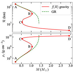
Figure 1: The variation of radius and central density with respect to the mass of the WD.

In this section, we discuss the strength of GW emitted from an $f(R)$ gravity induced isolated WD. We earlier showed that in the presence of $f(R)$ gravity with $f(R)=R+\alpha R^{2}(1-\gamma R)$, where $\alpha=3\times 10^{14}$ cm² and $\gamma=4\times 10^{16}$ cm², it is possible to obtain sub-Chandrasekhar limiting mass WDs as well as super-Chandrasekhar WDs, along with the regular WDs just varying the central density $\rho_{c}$ of the WDs (Kalita & Mukhopadhyay, 2018). We also showed that, with the chosen values of the parameters, this model is valid in terms of the solar system test (Guo, 2014). For demonstration, we recall the key results from that work, depicted in Figure 1, which shows the variation of radius $\mathcal{R}$ and $\rho_{c}$ with respect to $M$. WDs following GR are shown in green dashed line and the red solid line corresponds to the $f(R)$ gravity induced WDs. Indeed, there are some WDs, e.g., EG 50, GD 140, J2056-3014, etc. (Provencal et al., 1998; Lopes de Oliveira et al., 2020), which do not follow the standard Chandrasekhar mass–radius relation. Moreover, it is to be noted that we adopt the perturbative calculations and consider the exterior solution of the WD to be the Schwarzschild solution while obtaining the mass–radius curve in $f(R)$ gravity. As a result, $R$ is asymptotically flat outside the WD (Ganguly et al., 2014; Capozziello et al., 2016). Moreover, in perturbative analysis, a WD is unstable under the radial perturbation if it falls in the branch where $\partial M/\partial\rho_{c}<0$ ($\partial M/\partial\rho_{c}>0$ is known as the positivity condition, which is a necessary condition for stability) (Shapiro & Teukolsky, 1983; Glendenning, 2010). In perturbative method, while obtaining the mass–radius curve, $\partial M/\partial\rho_{c}>0$ still holds good to define the stability condition like GR, because any additional terms will be just perturbative corrections to the zeroth-order quantity which are usually small. From the figure, we observe that at low $\rho_{c}$, the effect of modified gravity is negligible, as both the curves overlap with each other (mostly in the branch AB). As $\rho_{c}$ increases, the mass–radius curve reaches a maximum at the mass $\sim 1M_{\odot}$ and $\rho_{c}\sim 1.5\times 10^{8}$ g cm^-3 (point B). Beyond this $\rho_{c}$, the curve turns back which violates the positivity condition and, hence, BC is an unstable branch. Therefore, point B corresponds to the sub-Chandrasekhar limiting mass WD. Further, reaching a minimum value, the curve again turns back from the point C, and quickly enters in the super-Chandrasekhar WD regime following $\partial M/\partial\rho_{c}>0$. Since the branch CD is stable, the super-Chandrasekhar WDs are stable under radial perturbation. The maximum $\rho_{c}$ is chosen in such a way that it does not violate any of the known physics for CO WDs, such as neutron drip (Shapiro & Teukolsky, 1983), pycno-nuclear reactions and inverse beta decay (Otoniel et al., 2019), etc. The empirical relation between $\mathcal{R}$ and $M$, in the branch AB is approximately $\mathcal{R}\propto M^{-2/5}$, in the branch BC is $\mathcal{R}\propto M$, and that of in the branch CD is $\mathcal{R}\propto M^{-1/2}$. In this way, this form of $f(R)$ gravity, with the chosen parameters, can explain both the sub- and super-Chandrasekhar limiting mass WDs just by varying the $\rho_{c}$. It is however evident that there is no super-Chandrasekhar mass-limit in this model. Such a mass-limit is possible if we consider higher-order corrections (at least $16^{\mathrm{th}}$ order) to the Starobinsky model as discussed earlier (Kalita & Mukhopadhyay, 2018). The beauty of this model is that at the low-density limit, the extra terms of modified gravity have a negligible effect, and GR is enough to describe the underlying physics. In the case of a star, its density is relatively small compared to the WD’s density and, hence, even if the same $\alpha$ and $\gamma$ remain intact, their effect is not prominent in the star phase. It brings in significant effect only when the star becomes a WD depending on the density. Now, based on this mass–radius relation, we discuss the corresponding strength of GW separately for each of the possibilities, mentioned in the previous section.

4.1 Presence of roughness at WD’s surface

We have already mentioned that if a pre-existed tri-axial WD rotates, it can produce continuous gravitational radiation. One possibility for a WD of being tri-axial is due to the asymmetry of matter present at its surface. One can imagine this configuration as a similar structure of the earth or moon, where there are mountains and craters (holes) at the surface. We assume that there are excess ‘mountains’ along the $x-$axis and ‘holes’ along the $z-$axis of a WD, as shown in Figure 2. Such a configuration guarantees a tri-axial system with $I_{1}<I_{2}<I_{3}$. For simplicity, we assume $\Omega_{1}=\Omega_{2}=\Omega_{3}$.

Figure 2: Exaggerated figure of the presence of mountains and holes at the surface of a WD.

Let us now check the maximum possible height of a mountain on a WD’s surface. Assuming the mountains to be generated due to the shear in the outer envelope of WDs (same as the case for the earth where there are mountains at its crust), the maximum height of a mountain is given by (Sedrakian et al., 2005)

$$H=\frac{S}{\rho g},$$ (36)

where $\rho$ is the average density of the mountain, $g$ the acceleration due to gravity at the surface of the WD, and $S$ the shear modulus which is given by (Mott & Jones, 1958; Baym & Pines, 1971)

$$S=0.295~{}Z^{2}e^{2}n_{e}^{4/3},$$ (37)

with $e$ being the charge of an electron, $Z$ the atomic number, and $n_{e}$ the electron number density in the mountain. Substituting this expression, the maximum height of the mountain reduces to

$$H=3.637\times 10^{12}\frac{Z^{2}}{g}\rho^{1/3}~{}\mathrm{cm}.$$ (38)

Assuming the C-O WDs with the surface mostly consisting of He, we choose $Z=2$. Moreover, assuming the mountains’ average density to be the density just below the surface of the WDs, i.e. $\rho\approx 10^{-6}\rho_{c}$, we obtain $H$ for various WDs with different values of $\rho_{c}$, which is shown in Figure 3. From the empirical relations mentioned in the previous section, we also obtain the same between $H$ and $M$: in the branch AB, $H\propto M^{-2/5}$, in CD, $H\propto M^{-7/6}$, while in BC, $H$ is nearly constant.

Figure 3: The maximum height of a mountain present on a WD as a function of mass.

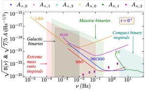
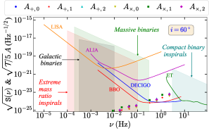
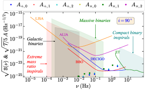
Figure 4: $\sqrt{\mathcal{T}/5}A$ for $f(R)$ gravity induced WDs with rough surfaces for different $i$ over 5 s integration time along with various detectors’ PSD.

It is evident from Figure 3 that $H\ll\mathcal{R}$. However, if there is a series of mountains of similar heights on the $x-$direction and big holes on the $z-$direction, as shown in Figure 2, effective radii of the WDs alter. The effective radii in $x-$, $y-$ and $z-$directions become $\mathcal{R}+H$, $\mathcal{R}$ and $\mathcal{R}-H$ respectively, resulting in a tri-axial system. Hence, the moments of inertia along different directions are given by

$$I_{1} =\frac{M}{5}\left[\mathcal{R}^{2}+\left(\mathcal{R}-H\right)^{2}\right],$$ (39)

$$I_{2} =\frac{M}{5}\left[\left(\mathcal{R}+H\right)^{2}+\left(\mathcal{R}-H\right)^{2}\right],$$

$$I_{3} =\frac{M}{5}\left[\mathcal{R}^{2}+\left(\mathcal{R}+H\right)^{2}\right].$$

Moreover, we know that rotation can also increase the mass and radius of a WD. Hence, we assume the angular frequency to be $1/10$th of the maximum possible angular frequency, i.e., $\Omega=1/10\sqrt{GM/\mathcal{R}^{3}}$, such that it does not affect the mass and size of the WD. Using the set of Equations (26), we obtain the dimensionless strain amplitude of GW, $A$ (e.g., $A_{+,0}$, $A_{\times,0}$, etc.), emitted from WDs with rough surface, corresponding to all three frequencies of the spectrum. Moreover, we know that the integrated signal to noise ratio (SNR) increases if we observe the source for a long period of time $\mathcal{T}$. The relation between SNR and $\mathcal{T}$ is given by (Maggiore, 2008; Thrane & Romano, 2013; Sieniawska & Bejger, 2019)

$$\mathrm{SNR}=\frac{1}{\sqrt{5}}\left(\frac{\mathcal{T}}{\mathtt{S}(\nu)}\right)^{1/2}A,$$ (40)

where $\mathtt{S}(\nu)$ is the power spectral density (PSD) at a frequency $\nu$. We show PSD of various detectors as a function of frequency (Sathyaprakash & Schutz, 2009; Moore et al., 2015) in Figure 4, along with $\sqrt{\mathcal{T}/5}A$ for $f(R)$ gravity induced WDs with $\rho_{c}=10^{6},10^{7},10^{8},10^{9},10^{10},1.66\times 10^{10}$ g cm^-3 over $\mathcal{T}=5$ s assuming $r=100$ pc. It is evident that many of these dense WDs will readily, or at most in a few seconds, be detected by DECIGO and BBO with $\mathrm{SNR}\gtrsim 5$. Since the signal is continuously emitted for a long duration, the significantly super-Chandrasekhar WDs, being smaller in size, can also be detected by the Einstein Telescope with $\mathrm{SNR}\approx 5$ if the signal is integrated over $\mathcal{T}\sim 102$ mins. However, to detect these WDs by ALIA or LISA with the same SNR, the integration time turns out to be $\mathcal{T}\sim 3$ months and $\mathcal{T}\sim 40000$ yrs respectively. Hence, it seems impossible for LISA to detect the GW signal from WDs with rough surfaces. Figure 5(a) shows $\sqrt{\mathcal{T}/5}A$ for different integration times for these WDs. It is evident from this figure that SNR increases as the integration time increases, allowing possibility of detecting these WDs even by the Einstein Telescope and ALIA. Furthermore, due to the emission of gravitational radiation, it is associated with the quadrupolar luminosity, given by (Zimmermann, 1980)

$$L_{\text{GW}} =-\derivative{E}{t}=-I_{3}\Omega_{\text{rot}}\dot{\Omega}_{\text{rot}}$$

$$\approx\frac{32G}{5c^{5}}b^{6}\left(I_{2}-I_{1}\right)^{2}+\frac{2G}{5c^{5}}a^{2}b^{4}\left(I_{3}-\frac{I_{1}+I_{2}}{2}\right)^{2}.$$ (41)

Since there is no magnetic field in this WD configuration, there will be no associated electromagnetic counterpart. In other words, these WDs do not emit any dipole radiation. Nevertheless, due to the emission of GW radiation, the WD starts spinning down, i.e., $\Omega_{\text{rot}}$ decreases with time. After a certain period of time (characteristic timescale, $P$, of a WD pulsar), it will lose all its rotational energy and can no longer radiate any gravitational radiation. Using the expression for $L_{\text{GW}}$, we obtain

$$P\approx\frac{135I_{3}c^{5}}{2G\Omega_{\text{rot}}^{4}}\frac{1}{64Y^{3}\left(I_{2}-I_{1}\right)^{2}+XY^{2}\left(2I_{3}-I_{1}-I_{2}\right)^{2}},$$ (42)

with

$$X=1+\frac{I_{2}(I_{3}-I_{2})}{I_{1}(I_{3}-I_{1})}~{}~{}\mathrm{and}~{}~{}Y=1+\frac{I_{2}(I_{2}-I_{1})}{I_{3}(I_{3}-I_{1})}.$$

Figure 6 shows the variation of $L_{\text{GW}}$ and $P$ with respect to $M$ of WD. The empirical relations for $L_{\text{GW}}$ and $P$ in various branches are given in Table 1. It is evident that the life-time of massive WD pulsars is shorter than that of the lighter WDs.

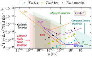
(a)  WDs with surface roughness.

(b)  WDs with magnetic field.

Figure 5: $\sqrt{\mathcal{T}/5}A$ for $f(R)$ gravity induced WDs with $i=30\degree$ and different integration time along with various detectors’ PSD.

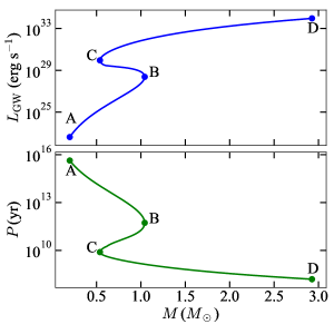
Figure 6: The variation of $L_{\text{GW}}$ and $P$ with respect to the mass of WD with mountains and holes.

Table 1: The empirical relations of various quantities with respect to mass of the WDs.

Quantity	AB branch	BC branch	CD branch
Radius	$\mathcal{R}\propto M^{-2/5}$	$\mathcal{R}\propto M$	$\mathcal{R}\propto M^{-1/2}$
Maximum height	$H\propto M^{-2/5}$	$H\approx$ constant	$H\propto M^{-7/6}$
Luminosity	$L_{\text{GW}}\propto M^{3}$	$L_{\text{GW}}\approx$ constant	$L_{\text{GW}}\propto M^{5/2}$
Timescale	$P\propto M^{-23/5}$	$P\propto M$	$P\propto M^{-5}$

4.2 Presence of magnetic field in WD

Figure 7: Cartoon diagram of a magnetized WD with magnetic field is along $z^{\prime}-$axis and rotation is along $z-$axis.

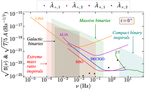
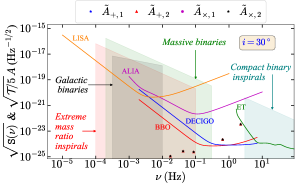
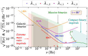
Figure 8: $\sqrt{\mathcal{T}/5}A$ for $f(R)$ gravity induced weakly magnetized WD pulsars for different $i$ over 5 s integration time along with various detectors’ PSD.

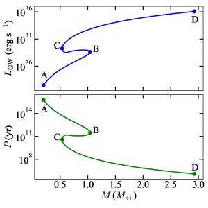
Figure 9: Same as Figure 6 except that the WDs have magnetic field instead of mountains.

As mentioned in the previous section, if a magnetized WD rotates with a misalignment between its magnetic field and rotation axes (similar configuration of a pulsar), it can emit continuous GW. We already provided a detailed discussion on GW emitted from WDs with different magnetic field geometries and strengths in GR (Kalita & Mukhopadhyay, 2019b; Kalita et al., 2020). Figure 7 shows an illustrative diagram of a magnetized WD where the magnetic field is along $z^{\prime}-$axis and rotation is along the $z-$axis, with $\chi$ being the angle between these two axes. We calculate the amplitude of GW using the set of Equations (34) assuming the difference in radii of the WD between those along $x-$ and $z-$axes be $0.01\%$, i.e., $\epsilon=\absolutevalue{I_{3}-I_{1}}/I_{3}\approx 2\times 10^{-4}$, due to the presence of a very weak magnetic field and slow rotation. The choice of weak fields and slow rotation assures that the underlying WD mass–radius solutions do not practically differ from the solutions based on the $f(R)$ gravity without magnetic fields and rotation. In future, we plan to check rigorously by solving the set of equations, if indeed such $\epsilon$ is possible in the presence of weak magnetic fields and rotation keeping the mass and radius practically intact. As we will show below, however, the chosen $\epsilon$ appears to be minimally required value to have any appreciable effect. Nevertheless, there are examples of weakly magnetized WD pulsars, which can be explained even in GR framework, e.g. AE Aquarii (Bookbinder & Lamb, 1987), AR Scorpii (Marsh et al., 2016), where magnetic fields hardly affect their mass–radius relations. Figure 8 shows PSD as a function of frequency for various detectors along with $\sqrt{\mathcal{T}/5}A$ over 5 s integration time for various $f(R)$ gravity induced WD pulsars with different $i$ assuming $\chi=90\degree$ and $r=100$ pc. It is evident that while DECIGO and BBO can immediately detect such weakly magnetized super-Chandrasekhar WDs, the Einstein Telescope can detect them in $\mathcal{T}\sim 6$ mins with $\mathrm{SNR}\approx 5$ (see Figure 5(b)). However, for ALIA and LISA, the corresponding integration time respectively turns out to be $\mathcal{T}\sim 5$ days and $\mathcal{T}\sim 25000$ yrs. Hence, it is also possible to detect such weakly magnetized WDs using ALIA, whereas for LISA, it is quite impossible. Figure 5(b) depicts $\sqrt{\mathcal{T}/5}A$ for these WDs with different integration times to show that SNR increases if the integration time increases so that various detectors can detect them eventually. For such a system, the GW luminosity is given by (Zimmermann & Szedenits, 1979)

$$L_{\text{GW}}\approx\frac{2G}{5c^{5}}\left(I_{3}-I_{1}\right)^{2}\Omega^{6}\sin^{2}\chi\left(1+15\sin^{2}\chi\right).$$ (43)

It is expected that a source can emit electromagnetic radiation in the presence of a magnetic field, and it is the dipole radiation in the case of a WD pulsar. However, because of the presence of a weak magnetic field, the dipole radiation emitted from such a WD is minimal, and the corresponding dipole luminosity is negligible as compared to $L_{\text{GW}}$. Hence the spin-down timescale is mostly governed by $L_{\text{GW}}$, given by (Kalita et al., 2020)

$$P\approx\left(\frac{5I_{3}c^{5}}{8G\left(I_{3}-I_{1}\right)^{2}\Omega^{4}}\right)\frac{1}{\sin^{2}\chi\left(1+15\sin^{2}\chi\right)}.$$ (44)

Figure 9 shows the variation of $L_{\text{GW}}$ and $P$ with respect to $M$ for various WDs with $\chi=90\degree$. The maximum $L_{\text{GW}}$ in the case of a WD is $\sim 10^{37}$ erg s^-1. The empirical relations of $L_{\text{GW}}$ and $P$, in various branches, are same as the previous case provided in Table 1. It is also clear from the figure that the massive WD pulsars are short-lived as compared to the lighter ones.

5 Discussion

From Figures 4 and 8, we observe that the GW frequency of isolated WDs could be much larger as compared to that of galactic binaries. This is because, in the case of isolated WDs, the spin frequency is responsible for the GW generation, whereas, in the case of binaries, their orbital periods are essential. Therefore, the confusion noise of the binaries does not affect the detection of the isolated WDs. However, the GW frequency of some other sources, such as massive binaries and compact binary inspirals, is similar to that of isolated WDs. Hence, using specific templates for binaries, the objects can be distinguished from each other. Of course, the frequency range of isolated WDs is such that neither the nano-hertz detectors, such as IPTA, EPTA, and NANOGrav, nor the other currently operating ground-based detectors such as LIGO, VIRGO and KAGRA, can detect them.

From Figure 1, it is evident that the GR dominated WDs are considerably big as compared to the $f(R)$ gravity dominated ones, particularly at higher central densities, provided they possess the same central density. Moreover, using the equations (27) and (35), we have $h_{0}\propto I$ with $I$ being the typical moment of inertia of the body. As a result, if we compare two WDs with the same ellipticity and angular frequency, the GR dominated WD emits stronger gravitational radiation. Since this paper is dedicated to studying the effect of $f(R)$ gravity, we do not explicitly calculate $h_{0}$ in the case of GR, like we have calculated it in detail in our earlier papers (Kalita & Mukhopadhyay, 2019b, 2020; Kalita et al., 2020). Moreover, we target to explore the detectability of those WDs which exhibit sub- and super-Chandrasekhar limiting mass WDs in the same $M-\mathcal{R}$ relation, which GR based theory cannot, and it has many consequences outlined in the Introduction. However, it is to be noted that $f(R)$ gravity dominated WDs, being smaller in size, can rotate much faster with frequency $\gtrsim 1$ Hz, which is not possible in the case of a regular WD governed by GR. In this paper, we have shown that in the presence of small deformation, such as the presence of a rough surface or magnetic fields, these WDs can emit intense gravitational radiation, which can later possibly be detected by BBO, DECIGO, ALIA, and Einstein Telescope.

The birth rate of He-dominated WDs is $\sim 1.5\times 10^{-12}$ pc^-3 yr^-1 (Guseinov et al., 1983), which means within 100 pc radius, only one WD is formed in approximately $10^{6}$ yrs. Hence, continuous GW from some massive WDs, which have radiation timescales (life span) $\sim 10^{8-9}$ yrs, can be detected, as shown in the Figures 4 and 8. If the advanced futuristic detectors, such as DECIGO, BBO, or Einstein Telescope detect the isolated WDs, one can quickly check whether the physics is governed by GR, or $f(R)$ gravity, or any other modified theory of gravity as follows. Once the GW detectors detect such a WD, we have the information of $h_{0}$ and $\Omega_{\text{rot}}$. Consequently, if the distance to the source $r$ is known by some other method, then by using the Equations (27) and (35), one can estimate the ellipticity and, thereby, can predict the mass and size of the WD. This will be a direct detection of the WD with low thermal luminosity (usually a super-Chandrasekhar WD which is smaller in size). In this way, we obtain the exact mass–radius relation of the WD. Since different theories provide different mass–radius relations of the WD, by obtaining the exact mass–radius relation from observation, one can rule out various theories from the zoo of modified theories of gravity which do not follow this relation. For example, Figure 10 shows mass–radius relations for a particular $f(R)$ gravity model but with different sets of model parameters. Comparing these results with those shown in Figure 1 reveals that the range of radius for stable WDs depends on the chosen model parameters for the same ranges of mass and central density. Direct detection of the WDs will provide valuable information to identify the correct radius range and hence mass–radius relation of the WDs.

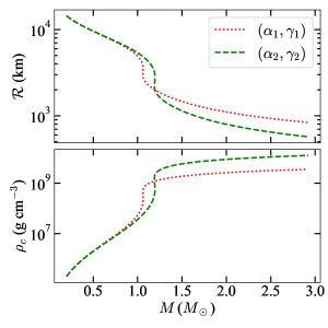
Figure 10: $M-\mathcal{R}$ and $M-\rho_{c}$ relations for WDs for $f(R)=R+\alpha R^{2}(1-\gamma R)$ model. The values of $\alpha$ and $\gamma$ in the units of cm² are $(\alpha_{1},\gamma_{1})=(10^{14},10^{17})$ and $(\alpha_{2},\gamma_{2})=(3\times 10^{14},3\times 10^{17})$.

6 Conclusions

In this paper, we have established a link between theory and possible GW observations of the WDs in a $f(R)$ gravity. Various researchers have already proposed hundreds of modified theories of gravity, including many $f(R)$ gravity theories, and each one of them possesses its own peculiarity. However, because of the lack of advanced observations near extremely high gravity regime, nobody, so far, can rule out most of the models to single out one specific theory of gravity. In this paper, we consider one valid class of $f(R)$ gravity model from the solar system constraints, which can explain both the sub- and super-Chandrasekhar WDs, along with the normal WDs, depending only on their central densities keeping the parameters of the model fixed. However, from the point of observation, the primary difficulty is that we do not know the size of the peculiar WDs and, hence, the exact mass–radius curve is still unknown. Thereafter, we calculate the strength of GW emitted from these WDs, assuming they slowly rotate with little deformation due to some other factors, such as the presence of roughness of the envelope, or the presence of a weak magnetic field. If the advanced futuristic GW detectors, such as ALIA, DECIGO, BBO, or Einstein Telescope can detect these WDs, one can estimate the ellipticity of the WDs and, thereby, put bounds on the WD’s size. This will restrict the mass–radius relation of the WD, which can rule out various modified theories, and we will be inching towards the ultimate theory of gravity.

References

- Astashenok et al. (2013) Astashenok, A. V., Capozziello, S., & Odintsov, S. D. 2013, J. Cosmology Astropart. Phys, 12, 040
- Astashenok et al. (2014) —. 2014, Phys. Rev. D, 89, 103509
- Banerjee et al. (2020a) Banerjee, I., Chakraborty, S., & SenGupta, S. 2020a, Phys. Rev. D, 101, 041301
- Banerjee et al. (2020b) Banerjee, I., Sau, S., & SenGupta, S. 2020b, Phys. Rev. D, 101, 104057
- Baym & Pines (1971) Baym, G., & Pines, D. 1971, Annals of Physics, 66, 816
- Belyaev et al. (2015) Belyaev, V. B., Ricci, P., Šimkovic, F., et al. 2015, Nuclear Physics A, 937, 17
- Berry & Gair (2011) Berry, C. P. L., & Gair, J. R. 2011, Phys. Rev. D, 83, 104022
- Bertolami & Mariji (2016) Bertolami, O., & Mariji, H. 2016, Phys. Rev. D, 93, 104046
- Bhattacharya et al. (2018) Bhattacharya, M., Mukhopadhyay, B., & Mukerjee, S. 2018, MNRAS, 477, 2705
- Bonazzola & Gourgoulhon (1996) Bonazzola, S., & Gourgoulhon, E. 1996, A&A, 312, 675
- Bookbinder & Lamb (1987) Bookbinder, J. A., & Lamb, D. Q. 1987, ApJ, 323, L131
- Braithwaite (2009) Braithwaite, J. 2009, MNRAS, 397, 763
- Burrage & Sakstein (2018) Burrage, C., & Sakstein, J. 2018, Living Reviews in Relativity, 21, 1
- Cao et al. (2016) Cao, Y., Johansson, J., Nugent, P. E., et al. 2016, ApJ, 823, 147
- Capozziello et al. (2008) Capozziello, S., Corda, C., & de Laurentis, M. F. 2008, Physics Letters B, 669, 255
- Capozziello et al. (2016) Capozziello, S., De Laurentis, M., Farinelli, R., & Odintsov, S. D. 2016, Phys. Rev. D, 93, 023501
- Casas et al. (2017) Casas, S., Kunz, M., Martinelli, M., & Pettorino, V. 2017, Physics of the Dark Universe, 18, 73
- Chandrasekhar (1931) Chandrasekhar, S. 1931, ApJ, 74, 81
- Chandrasekhar (1935) —. 1935, MNRAS, 95, 207
- Choudhuri (2010) Choudhuri, A. R. 2010, Astrophysics for Physicists (Cambridge University Press)
- Das & Mukhopadhyay (2013) Das, U., & Mukhopadhyay, B. 2013, Phys. Rev. Lett., 110, 071102
- Das & Mukhopadhyay (2014) —. 2014, J. Cosmology Astropart. Phys, 2014, 050
- Das & Mukhopadhyay (2015) —. 2015, J. Cosmology Astropart. Phys, 5, 045
- Dass & Liberati (2019) Dass, A., & Liberati, S. 2019, General Relativity and Gravitation, 51, 84
- De Felice & Tsujikawa (2010) De Felice, A., & Tsujikawa, S. 2010, Living Reviews in Relativity, 13, 3
- Filippenko et al. (1992) Filippenko, A. V., Richmond, M. W., Branch, D., et al. 1992, AJ, 104, 1543
- Ganguly et al. (2014) Ganguly, A., Gannouji, R., Goswami, R., & Ray, S. 2014, Phys. Rev. D, 89, 064019
- Garnavich et al. (2004) Garnavich, P. M., Bonanos, A. Z., Krisciunas, K., et al. 2004, ApJ, 613, 1120
- Glendenning (2010) Glendenning, N. 2010, Special and General Relativity: With Applications to White Dwarfs, Neutron Stars and Black Holes, Astronomy and Astrophysics Library (Springer New York)
- Gong & Hou (2018) Gong, Y., & Hou, S. 2018, Universe, 4, 85
- Guo (2014) Guo, J.-Q. 2014, International Journal of Modern Physics D, 23, 1450036
- Gupta et al. (2020) Gupta, A., Mukhopadhyay, B., & Tout, C. A. 2020, MNRAS, 496, 894
- Guseinov et al. (1983) Guseinov, O. K., Novruzova, K. I., & Rustamov, I. S. 1983, Ap&SS, 97, 305
- Hachisu et al. (2012) Hachisu, I., Kato, M., Saio, H., & Nomoto, K. 2012, ApJ, 744, 69
- Held et al. (2019) Held, A., Gold, R., & Eichhorn, A. 2019, J. Cosmology Astropart. Phys, 2019, 029
- Hicken et al. (2007) Hicken, M., Garnavich, P. M., Prieto, J. L., et al. 2007, ApJ, 669, L17
- Hillebrandt & Niemeyer (2000) Hillebrandt, W., & Niemeyer, J. C. 2000, ARA&A, 38, 191
- Howell et al. (2006) Howell, D. A., Sullivan, M., Nugent, P. E., et al. 2006, Nature, 443, 308
- Jana & Mohanty (2019) Jana, S., & Mohanty, S. 2019, Phys. Rev. D, 99, 044056
- Joyce et al. (2016) Joyce, A., Lombriser, L., & Schmidt, F. 2016, Annual Review of Nuclear and Particle Science, 66, 95
- Kalita & Mukhopadhyay (2018) Kalita, S., & Mukhopadhyay, B. 2018, J. Cosmology Astropart. Phys, 9, 007
- Kalita & Mukhopadhyay (2019a) —. 2019a, European Physical Journal C, 79, 877
- Kalita & Mukhopadhyay (2019b) —. 2019b, MNRAS, 490, 2692
- Kalita & Mukhopadhyay (2020) —. 2020, IAU Symposium, 357, 79
- Kalita et al. (2020) Kalita, S., Mukhopadhyay, B., Mondal, T., & Bulik, T. 2020, ApJ, 896, 69
- Kamiya et al. (2012) Kamiya, Y., Tanaka, M., Nomoto, K., et al. 2012, ApJ, 756, 191
- Katsuragawa et al. (2019) Katsuragawa, T., Nakamura, T., Ikeda, T., & Capozziello, S. 2019, Phys. Rev. D, 99, 124050
- Kausar et al. (2016) Kausar, H. R., Philippoz, L., & Jetzer, P. 2016, Phys. Rev. D, 93, 124071
- Khokhlov et al. (1993) Khokhlov, A., Mueller, E., & Hoeflich, P. 1993, A&A, 270, 223
- Komatsu et al. (1989) Komatsu, H., Eriguchi, Y., & Hachisu, I. 1989, MNRAS, 237, 355
- Landau & Lifshitz (1982) Landau, L., & Lifshitz, E. 1982, Mechanics: Volume 1, Vol. 1 (Elsevier Science)
- Liang et al. (2017) Liang, D., Gong, Y., Hou, S., & Liu, Y. 2017, Phys. Rev. D, 95, 104034
- Lieb & Yau (1987) Lieb, E. H., & Yau, H.-T. 1987, ApJ, 323, 140
- Liu et al. (2014) Liu, H., Zhang, X., & Wen, D. 2014, Phys. Rev. D, 89, 104043
- Liu et al. (2018) Liu, T., Zhang, X., & Zhao, W. 2018, Physics Letters B, 777, 286
- Lopes de Oliveira et al. (2020) Lopes de Oliveira, R., Bruch, A., Rodrigues, C. V., Oliveira, A. S., & Mukai, K. 2020, ApJ, 898, L40
- Maggiore (2008) Maggiore, M. 2008, Gravitational waves: Volume 1: Theory and experiments, Vol. 1 (Oxford university press)
- Marsh et al. (2016) Marsh, T. R., Gänsicke, B. T., Hümmerich, S., et al. 2016, Nature, 537, 374
- Martin et al. (2006) Martin, R. G., Tout, C. A., & Lesaffre, P. 2006, MNRAS, 373, 263
- Mazzali et al. (1997) Mazzali, P. A., Chugai, N., Turatto, M., et al. 1997, MNRAS, 284, 151
- Modjaz et al. (2001) Modjaz, M., Li, W., Filippenko, A. V., et al. 2001, PASP, 113, 308
- Moffat (2020) Moffat, J. W. 2020, arXiv e-prints, arXiv:2008.04404
- Moore et al. (2015) Moore, C. J., Cole, R. H., & Berry, C. P. L. 2015, Classical and Quantum Gravity, 32, 015014
- Mott & Jones (1958) Mott, N., & Jones, H. 1958, The Theory of the Properties of Metals and Alloys, Dover books on physics and mathematical physics (Dover Publications)
- Multamäki & Vilja (2006) Multamäki, T., & Vilja, I. 2006, Phys. Rev. D, 74, 064022
- Näf & Jetzer (2010) Näf, J., & Jetzer, P. 2010, Phys. Rev. D, 81, 104003
- Nojiri et al. (2017) Nojiri, S., Odintsov, S. D., & Oikonomou, V. K. 2017, Phys. Rep., 692, 1
- Nomoto et al. (1997) Nomoto, K., Iwamoto, K., & Kishimoto, N. 1997, Science, 276, 1378
- Ong (2018) Ong, Y. C. 2018, J. Cosmology Astropart. Phys, 9, 015
- Otoniel et al. (2019) Otoniel, E., Franzon, B., Carvalho, G. A., et al. 2019, ApJ, 879, 46
- Padmanabhan (2001) Padmanabhan, T. 2001, Theoretical Astrophysics, Vol. 2 (Cambridge University Press)
- Pakmor et al. (2010) Pakmor, R., Kromer, M., Röpke, F. K., et al. 2010, Nature, 463, 61
- Pérez et al. (2013) Pérez, D., Romero, G. E., & Perez Bergliaffa, S. E. 2013, A&A, 551, A4
- Prasia & Kuriakose (2014) Prasia, P., & Kuriakose, V. C. 2014, International Journal of Modern Physics D, 23, 1450037
- Provencal et al. (1998) Provencal, J. L., Shipman, H. L., Høg, E., & Thejll, P. 1998, ApJ, 494, 759
- Pun et al. (2008) Pun, C. S. J., Kovács, Z., & Harko, T. 2008, Phys. Rev. D, 78, 024043
- Ryder (2009) Ryder, L. 2009, Introduction to General Relativity (Cambridge University Press)
- Saio & Nomoto (2004) Saio, H., & Nomoto, K. 2004, ApJ, 615, 444
- Sathyaprakash & Schutz (2009) Sathyaprakash, B. S., & Schutz, B. F. 2009, Living Reviews in Relativity, 12, 2
- Sbisà et al. (2019) Sbisà, F., Piattella, O. F., & Jorás, S. E. 2019, Phys. Rev. D, 99, 104046
- Scalzo et al. (2012) Scalzo, R., Aldering, G., Antilogus, P., et al. 2012, ApJ, 757, 12
- Scalzo et al. (2010) Scalzo, R. A., Aldering, G., Antilogus, P., et al. 2010, ApJ, 713, 1073
- Sedrakian et al. (2005) Sedrakian, D. M., Hayrapetyan, M. V., & Sadoyan, A. A. 2005, Astrophysics, 48, 53
- Shapiro & Teukolsky (1983) Shapiro, S. L., & Teukolsky, S. A. 1983, Black holes, white dwarfs, and neutron stars: The physics of compact objects (John Wiley and sons)
- Sieniawska & Bejger (2019) Sieniawska, M., & Bejger, M. 2019, Universe, 5, 217
- Silverman et al. (2011) Silverman, J. M., Ganeshalingam, M., Li, W., et al. 2011, MNRAS, 410, 585
- Sotiriou & Faraoni (2010) Sotiriou, T. P., & Faraoni, V. 2010, Reviews of Modern Physics, 82, 451
- Sousa et al. (2020) Sousa, M. F., Coelho, J. G., & de Araujo, J. C. N. 2020, MNRAS, 492, 5949
- Stabile (2010) Stabile, A. 2010, Phys. Rev. D, 82, 064021
- Starobinsky (1980) Starobinsky, A. A. 1980, Physics Letters B, 91, 99
- Stritzinger et al. (2006) Stritzinger, M., Mazzali, P. A., Sollerman, J., & Benetti, S. 2006, A&A, 460, 793
- Tanaka et al. (2010) Tanaka, M., Kawabata, K. S., Yamanaka, M., et al. 2010, ApJ, 714, 1209
- Taubenberger et al. (2008) Taubenberger, S., Hachinger, S., Pignata, G., et al. 2008, MNRAS, 385, 75
- Taubenberger et al. (2011) Taubenberger, S., Benetti, S., Childress, M., et al. 2011, MNRAS, 412, 2735
- Thrane & Romano (2013) Thrane, E., & Romano, J. D. 2013, Phys. Rev. D, 88, 124032
- Turatto et al. (1998) Turatto, M., Piemonte, A., Benetti, S., et al. 1998, AJ, 116, 2431
- Vainio & Vilja (2017) Vainio, J., & Vilja, I. 2017, General Relativity and Gravitation, 49, 99
- Van Den Broeck (2005) Van Den Broeck, C. 2005, Classical and Quantum Gravity, 22, 1825
- Will (2014) Will, C. M. 2014, Living Reviews in Relativity, 17, 4
- Yamanaka et al. (2009) Yamanaka, M., Kawabata, K. S., Kinugasa, K., et al. 2009, ApJ, 707, L118
- Yang et al. (2011) Yang, L., Lee, C.-C., & Geng, C.-Q. 2011, J. Cosmology Astropart. Phys, 2011, 029
- Yuan et al. (2010) Yuan, F., Quimby, R. M., Wheeler, J. C., et al. 2010, ApJ, 715, 1338
- Zimmermann (1980) Zimmermann, M. 1980, Phys. Rev. D, 21, 891
- Zimmermann & Szedenits (1979) Zimmermann, M., & Szedenits, Jr., E. 1979, Phys. Rev. D, 20, 351