Library-based Fast Algorithm for Simulating the Hodgkin-Huxley Neuronal Networks

Abstract

We present a modified library-based method for simulating the Hodgkin-Huxley (HH) neuronal networks. By pre-computing a high resolution data library during the interval of an action potential (spike), we can avoid evolving the HH equations during the spike and can use a large time step to raise efficiency. The library method can stably achieve at most 10 times of speedup compared with the regular Runge-Kutta method while capturing most statistical properties of HH neurons like the distribution of spikes which data is widely used in the statistical analysis like transfer entropy and Granger causality. The idea of library method can be easily and successfully applied to other HH-type models like the most prominent “regular spiking”, “fast spiking”, “intrinsically bursting” and “low-threshold spike” types of HH models.

Keywords Library method; Hodgkin-Huxley networks; Efficiency; Fast algorithm

1 Introduction

The Hodgkin-Huxley (HH) model [1, 2, 3], originally proposed to describe the behavior of the giant axon, is one of the most realistic models. It is then regarded as the foundation for other neuronal models with more complicated behaviors like bursting and adaptation. Because of its complexity, we often use regular Runge-Kutta scheme in the numerical simulation to study the dynamics of this model. However the HH equations become stiff when the neuron fires a spike. As a consequence, we have to take a sufficiently small time step to avoid stability problems. But we need to simulate the model quite frequently to study its properties with different aims. Sometimes we even need to simulate the model with hundreds of neurons for hours to record the spikes or voltages [4, 5]. Therefore, it is important to find a fast algorithm to simulate the model.

The stiff part during a firing event is from the activities of its sodium and potassium ion channels and can last for about 3 ms. We offer a library method to deal with the stiff period and it can use much larger time steps compared with the regular Runge-Kutta method. The library method treats a HH neuron as an I&F one. Once a HH neuron’s membrane potential reaches the threshold, we stop evolving its HH equations and restart after the stiff part. The time-courses of membrane potential and gating variables during the stiff part can be recovered from a pre-computed high resolution data library. So once the membrane potential reaches the threshold, we record its state and decide the restart state interpolated from the data library. Therefore, we can avoid the stiff part and use a large time step to evolve the HH model. The library method can use time steps one order of magnitude larger than the regular Runge-Kutta method while achieving precise statistical information of the HH model, $e.g.$, the distribution of spikes. Recently, statistical tools like Granger causality, transfer entropy and maximum entropy have been proven to be effective in probing neural interactions, $e.g.$, detecting causality, identifying effective connectivity and reconstructing the fire patterns [4, 6, 5, 7]. These works are mainly based on the spike trains recorded for $\sim 20$ minutes to obtain an accurate distribution. We specially point out that the library method can stably speed up at most 10 times compared with the regular Runge-Kutta methods, which may make the HH model attractive as a base model in these statistical tools.

We emphasize that we should take into account the causality of synaptic spikes within a single time step. In general, when we evolve the HH neurons for one time step in the regular Runge-Kutta methods [8, 9], we only use the feedforward input during the time step. Without knowing when and which neurons will fire during the time step, we have to wait until the end of the evolution of this time step to consider the effect of these possible synaptic spikes. This approach may work well with a sufficiently small time step that there are only $O(1)$ spikes during one time step and the causal effect is negligible. However, when we use a large time step, the first spikes may influence the network via the spike-spike interactions that some extra spikes may appear if the first spikes are excitatory and some latter spikes may vanish otherwise. Therefore, to use a large time step, we should take the spike-spike correction procedure [10] to obtain accurate spike sequences.

We also investigate the validity of the library method in more complicated HH-type models with more voltage-dependent currents. They are the four most prominent types: “fast spiking”, “regular spiking”, “intrinsically bursting” and “low-threshold spike” [11, 12]. For each type of model, we build and use the data library in the same way as that in the standard HH model. The library method can still achieve accurate statistical information of these HH-type models with remarkable computational speedup.

2 Materials and methods

2.1 HH model

The dynamics of the $i$th neuron of an excitatory Hodgkin-Huxley (HH) neuronal network is governed by

$$\begin{cases}\begin{aligned} C\frac{dV_{i}}{dt}&=-(V_{i}-V_{\textrm{Na}})G_{\textrm{Na}}m_{i}^{3}h_{i}-(V_{i}-V_{\textrm{K}})G_{\textrm{K}}n_{i}^{4}-(V_{i}-V_{\textrm{L}})G_{\textrm{L}}+I_{i}^{\textrm{input}}\\ \frac{dm_{i}}{dt}&=(1-m_{i})\alpha_{m}(V_{i})-m_{i}\beta_{m}(V_{i})\\ \frac{dhi}{dt}&=(1-h_{i})\alpha_{h}(V_{i})-h_{i}\beta_{h}(V_{i})\\ \frac{dn_{i}}{dt}&=(1-n_{i})\alpha_{n}(V_{i})-n_{i}\beta_{n}(V_{i})\end{aligned}\end{cases}$$ (1)

where $V_{i}$ is the membrane potential, $m_{i}$, $h_{i}$ and $n_{i}$ are gating variables, $I_{i}^{\textrm{input}}$ is the input current, $\alpha$ and $\beta$ are empirical functions of $V$,

$$\alpha_{m}(V_{i})=\frac{0.1V_{i}+4}{1-\exp(-0.1V_{i}-4)} \beta_{m}(V_{i})=4\exp(-(V_{i}+65)/18)$$ (2)

$$\alpha_{h}(V_{i})=0.07\exp(-(V_{i}+65)/20) \beta_{h}(V_{i})=\frac{1}{1+\exp(-3.5-0.1V_{i})}$$

$$\alpha_{n}(V_{i})=\frac{0.01V_{i}+0.55}{1-\exp(-0.1V_{i}-5.5)} \beta_{n}(V_{i})=0.125\exp(-(V_{i}+65)/80)$$

Other parameters are constants: $C=1\mu\textrm{F$\cdot$cm}^{-2}$ is the membrane capacitance; $V_{\textrm{Na}}=50$ mV, $V_{\textrm{K}}=-77$ mV and $V_{\textrm{L}}=-54.387$ mV are reversal potentials; $G_{\textrm{Na}}=120\textrm{ mS$\cdot$cm}^{-2}$, $G_{\textrm{K}}=36\textrm{ mS$\cdot$cm}^{-2}$, and $G_{\textrm{L}}=0.3\textrm{ mS$\cdot$cm}^{-2}$ are the maximum conductances.

The input current $I_{i}^{\textrm{input}}$ is given by $I_{i}^{\textrm{input}}=-G_{i}(t)(V_{i}-V_{G})$ with

$$\frac{dG_{i}(t)}{dt}=-\frac{G_{i}(t)}{\sigma_{\textrm{r}}}+H_{i}(t)$$ (3)

$$\frac{dH_{i}(t)}{dt}=-\frac{H_{i}(t)}{\sigma_{\textrm{d}}}+f\sum_{l}\delta(t-s_{il})+\sum_{j\neq i}\sum_{l}S_{ij}\delta(t-\tau_{jl})$$ (4)

where $V_{\textrm{G}}$ is the reversal potential with value $V_{\textrm{G}}=0$ mV, $G_{i}(t)$ is the conductance, $H_{i}(t)$ is an additional parameter to describe $G_{i}(t)$, $\sigma_{\textrm{r}}$ and $\sigma_{\textrm{d}}$ are fast rise and slow decay time scale, respectively, and $\delta(\cdot)$ is the Dirac delta function. In this Letter, we use $\sigma_{\textrm{r}}=0.5$ ms, $\sigma_{\textrm{d}}=3.0$ ms. The second term in Eq. (4) is the feedforward input with magnitude $f$. The input time $s_{il}$ is generated from a Poisson process with rate $\nu$. The third term in Eq. (4) is the synaptic current from synaptic interactions in the network, where $S_{ij}$ is the coupling strength from the $j$th neuron to the $i$th neuron, $\tau_{jl}$ is the $l$th spike time of $j$th neuron.

When the voltage $V_{i}$, evolving continuously according to Eq. (1), reaches the threshold $V^{\textrm{th}}$, we say the $i$th neuron fires a spike at this time. Instantaneously, all its postsynaptic neurons receive this spike and their corresponding parameter $H$ jumps by an appropriate amount, $\mathit{e.g.}$, $S_{ji}$ for the $j$th neuron. For the sake of simplicity, we mainly consider an all-to-all coupled network with $S_{ij}=S/N$, where $S$ is the coupling strength and $N$ is the number of neurons. The given methods can be easily extended to other types of networks, $\mathit{e.g.}$, with inhibitory neurons, randomly and inhomogeneously connected.

2.2 Numerical scheme

We first introduce the most widely used Runge-Kutta fourth-order scheme (RK4) with fixed time step $\Delta$t to evolve the HH model. Since the neurons interact with each other through the spikes by influencing of conductance of the postsynaptic neurons, it is important to obtain accurate spike sequences. Then, there are some issues need to be clarified in simulation. For example, how to determine the spike time accurately [8, 9]. Suppose the $i$th neuron fires a spike at time $\tilde{t}$ in $[t,t+\Delta t]$, a naive way to determine the spike time is to set $\tilde{t}=t+\Delta t$ and then an error of order $\Delta t$ is introduced. Therefore, the whole scheme is limited to the first-order. To solve this problem, we can use numerical interpolation schemes to decide the spike time more accurately [8, 9]. After evolving the trajectory of the $i$th neuron from $t$ to $t+\Delta t$, we can use the obtained values $V_{i}(t),V_{i}(t+\Delta t),\frac{dV_{i}}{dt}(t),\frac{dV_{i}}{dt}(t+\Delta t)$ to perform a cubic Hermite interpolation to decide the spike time. Then the whole scheme have an accuracy of fourth-order.

Another problem is the causality of the spike events [10]. A usually used strategy is to evolve the network (1), for example from $t$ to $t+\Delta t$, only considering the feedforward input within the time interval $[t,t+\Delta t]$. If some synaptic spikes are fired during this interval, they will be assigned at the end of the time step $t+\Delta t$. This strategy will lead to some problems. One is that since we assign the synaptic spikes at the end of the time step rather than the real spike times, the accuracy is limited to the first-order. Another problem is that the first few synaptic spikes may strongly influence the other spiking neurons by spike-spike interactions, especially in the simulation with a large time step, hence the rest of the synaptic spikes may be incorrect.

To solve this problem, we take the spike-spike correction procedure [10], which strategy is similar to the event-driven approach [13, 14, 15]. Suppose we evolve the all-to-all connected network from $t$ to $t+\Delta t$. Here is the details. We first preliminarily evolve the neurons in the network independently from $t$ to $t+\Delta t$ considering only the feedforward input. If any neuron fires a spike during this time interval, say the $i$th neuron, we denote the spike time by $t_{\textrm{fire}}^{(i)}$, along with the cubic Hermite interpolation to determine the spike time. If a neuron does not fire during $[t,t+\Delta t]$, still say the $i$-th neuorn, we then set $t_{\textrm{fire}}^{(i)}=t+\Delta t$. After obtaining all these $t_{\textrm{fire}}^{(i)}$ values independently, we find the minimum one, without loss of generality, say $t_{\textrm{fire}}^{(1)}$. If $t_{\textrm{fire}}^{(1)}=t+\Delta t$, then there are no synaptic spikes in $[t,t+\Delta t]$ and therefore, there is no causal problem and we accept the preliminary trajectories as the solution. Otherwise, $t_{\textrm{fire}}^{(1)}$ is the first synaptic spike in $[t,t+\Delta t]$ and there is no causal problem during $[t,t_{\textrm{fire}}^{(1)}]$. So we update all the neurons from $t$ to $t_{\textrm{fire}}^{(1)}$, at which time neuron 1 still has a firing event. Then we move on to start another loop to find the next first synaptic spike time in $[t_{\textrm{fire}}^{(1)},t+\Delta t]$ until the evolving is finished.

With the cubic Hermite interpolation and spike-spike correction, we give the regular RK4 scheme. For the easy of illustration, we use the vector

$$X_{i}(t)=(V_{i}(t),m_{i}(t),h_{i}(t),n_{i}(t),G_{i}(t),H_{i}(t))$$ (5)

to represent the state of the $i$th neuron. Details of the numerical algorithm to evolve the network from $t$ to $t+\Delta t$ is given in Algorithm 1.

Input: $t$, $\Delta t$, $\{X_{i}(t)\}$ and $\{s_{il}\}$

Output: $\{X_{i}(t+\Delta t)\}$ and $\{\tau_{il}\}$(if any fired)

Preliminarily evolve the network from $t$ to $t+\Delta t$ to find the first synaptic spike:

for $i=1$ to $N$ do

      Let $M$ denote the total number of feedforward spikes of the $i$th neuron within $[t,t+\Delta t]$ and sort them into an increasing list $\{T_{m}^{\text{sorted}}\}$. Then we extend this notation such that $T_{0}^{\text{sorted}}=t$ and $T_{M+1}^{\text{sorted}}=t+\Delta t$.

      

      for $m=1$ to $M+1$  do

            Advance the equations for the $i$th HH neuron from $T_{m-1}^{\text{sorted}}$ to $T_{m}^{\text{sorted}}$ using the standard RK4 scheme. Then update the conductance $H_{i}(T_{m}^{\text{sorted}})$ by adding $f$.

             if $V_{i}(T_{m-1}^{\text{sorted}})<V^{\textrm{th}}$, $V_{i}(T_{m}^{\text{sorted}})\geq V^{\textrm{th}}$ then

                  Find the spike time $t_{\text{fire}}^{(i)}$ by cubic Hermite interpolation using the values $V_{i}(T_{m-1}^{\text{sorted}})$, $V_{i}(T_{m}^{\text{sorted}})$, $\frac{dV_{i}}{dt}(T_{m-1}^{\text{sorted}})$ and $\frac{dV_{i}}{dt}(T_{m}^{\text{sorted}})$.

                  

            else

                  Set $t_{\text{fire}}^{(i)}=t+\Delta t$.

            

      

while The minimum of $\{t_{\text{fire}}^{(i)}\}<t+\Delta t$  do

      Suppose $t_{\text{fire}}^{(1)}$ is the minimum one.

       Evolve neuron 1 to $t_{\text{fire}}^{(1)}$, and generate a spike at this moment. Then update all the remaining neurons to $t_{\text{fire}}^{(1)}$.

       Preliminarily evolve the network from $t_{\text{fire}}^{(1)}$ to $t+\Delta t$ to find the next first synaptic spike.

We accept $\{X_{i}{(T_{M+1}^{\text{sorted}})}\}$ as the solution $\{X_{i}{(t+\Delta t)}\}$;

Algorithm 1 Regular RK4 algorithm

2.3 Library method

When a neuron fires a spike, the HH neuron equations are stiff for some milliseconds denoted by $T^{\textrm{stiff}}$, as shown in Fig 1. This stiff period requires a sufficiently small time step to avoid stability problem. Therefore, in the regular RK4 scheme, we have to use a relatively small time step, $\mathit{e.g.}$, the widely used $\Delta t=1/32$ ms. To overcome the limitation in time step, we propose a modified library method [16]. It is based on the regular RK4 scheme and has the advantage of using a large time step to raise efficiency, while having comparable accuracy in statistical quantifications, $\mathit{e.g.}$, mean firing rate and the spike pattern (Details are given in Section 3). The library method depends on the length of stiff period, which is experientially set $T^{\textrm{stiff}}=3.5$ ms, long enough to cover the stiff parts in general firing events.

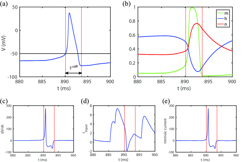
Figure 1: Typical firing event. (a) The trajectory of voltage $V$. The black line indicates the threshold $V^{\textrm{th}}$ and the red dotted lines indicate the stiff period. (b) The trajectory of $m,h,n$. (c) The trajectory of $\frac{dV}{dt}$ . (d) The trajectory of the input current $I_{i}^{\textrm{input}}$ ($\mu\textrm{A$\cdot$cm}^{-2}$). (e) The trajectory of the intrinsic current ($\mu\textrm{A$\cdot$cm}^{-2}$) which is the sum of ionic and leakage currents.

The library method [16] treats the HH neuron’s firing event like an I&F neuron. Once a neuron’s membrane potential reaches the threshold $V^{\textrm{th}}$, its voltage rises and reaches the peak value very quickly because of a large influx of the sodium current, then it drops back down to the lowest point by the potassium current. This process is actually an action potential and lasts for about 3 ms which is indeed the stiff period, as shown in Fig 1(a). If we have a pre-computed high resolution data library of $V,m,h,n$, we can recover their time-courses. In other words, once a neuron’s membrane potential reaches the threshold $V^{\textrm{th}}$, we stop evolving $V,m,h,n$ for the following stiff period $T^{\textrm{stiff}}$, and restart with the values interpolated from the library. Thus the stiff part is avoided and we can use a large time step to evolve the model to raise efficiency.

2.3.1 Build the library

Now we describe how to build the library in detail. Once a neuron’s membrane potential reaches the threshold $V^{\textrm{th}}$, we record the values $I^{\textrm{input}},m,h,n$ and denote them by $I^{\textrm{th}},m^{\textrm{th}},h^{\textrm{th}},n^{\textrm{th}}$, respectively. If we know the exact trajectory of $I^{\textrm{input}}$ for the following stiff period $T^{\textrm{stiff}}$, we can use a sufficiently small time step to evolve the Eq. (1) for $T^{\textrm{stiff}}$ with initial values $V^{\textrm{th}},m^{\textrm{th}},h^{\textrm{th}},n^{\textrm{th}}$ to obtain high resolution trajectories of $V,m,h,n$. We denote the obtained values after evolving by $V^{\textrm{re}},m^{\textrm{re}},h^{\textrm{re}},n^{\textrm{re}}$, where the superscript -re stands for the reset value.

However it is impossible to obtain the exact trajectory of $I^{\textrm{input}}$ without knowing the feedforward and synaptic spike information. As shown in Fig 1(d, e), $I^{\textrm{input}}$ varies during the stiff period with peak value in the range of $O(5)$ $\mu\textrm{A$\cdot$cm}^{-2}$, while the intrinsic current, the sum of ionic and leakage current, is about 30 $\mu\textrm{A$\cdot$cm}^{-2}$ at the spike time, and quickly rises to the peak value about 250 $\mu\textrm{A$\cdot$cm}^{-2}$, then stays at $O(-50)$ $\mu\textrm{A$\cdot$cm}^{-2}$ in the remaining stiff period. Therefore, the intrinsic current is dominant in the stiff period. With this observation, we keep $I^{\textrm{input}}$ as constant throughout the whole stiff period. We emphasize that this is the only assumption made in the library method. Then, given a suite of $I^{\textrm{th}},m^{\textrm{th}},h^{\textrm{th}},n^{\textrm{th}}$, we can obtain a suite of $V^{\textrm{re}},m^{\textrm{re}},h^{\textrm{re}},n^{\textrm{re}}$.

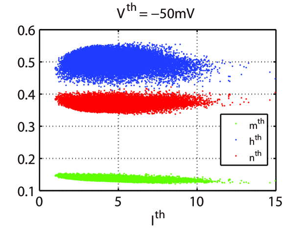
Figure 2: The ranges of values $I^{\textrm{th}},m^{\textrm{th}},h^{\textrm{th}},n^{\textrm{th}}$.

Before building the library, we choose $N_{I},N_{m},N_{h},N_{n}$ different values of $I^{\textrm{th}},m^{\textrm{th}},h^{\textrm{th}},n^{\textrm{th}}$, respectively, equally distributed in their ranges as shown in Fig 2. For each suite of $I^{\textrm{th}},m^{\textrm{th}},h^{\textrm{th}},n^{\textrm{th}}$, we evolve the Eq. (1) for a time interval of $T^{\textrm{stiff}}$ to obtain $V^{\textrm{re}},m^{\textrm{re}},h^{\textrm{re}},n^{\textrm{re}}$ with a sufficiently small time step, $\mathit{e.g.}$, $\Delta t=2^{-16}\approx 1.52\times 10^{-5}$ ms. Note that we should set $I^{\textrm{input}}$ constant $I^{\textrm{input}}=I^{\textrm{th}}$ throughout the whole time interval $T^{\textrm{stiff}}$. Then the data library is built with total size $8N_{I}N_{m}N_{h}N_{n}$. Larger values of $N_{I},N_{m},N_{h},N_{n}$ can increase the accuracy of the library and greatly increase the size of library at the same time. In our simulation, we take $N_{I}=21,N_{m}=16,N_{h}=21,N_{n}=16$, which can make the library sufficiently accurate as is shown in section 3. The library occupies only 6.89 megabyte in binary form and is quite small for today’s computers.

One key point in building the library is to choose a proper threshold value $V^{\textrm{th}}$. The threshold should be relatively low to keep the HH equations not stiff and allow a large time step with the stability requirement satisfied. On the other hand, it should be relatively high that a neuron will definitely fire a spike after its membrane potential reaches the threshold. In this Letter, we take $V^{\textrm{th}}=-50$ mV.

2.3.2 Use the library

We now illustrate how to use the library. Once a neuron’s membrane potential reaches the threshold, we first record the values $I^{\textrm{th}},m^{\textrm{th}},h^{\textrm{th}},n^{\textrm{th}}$, then stop evolving its HH equations of $V,m,h,n$ for the following $T^{\textrm{stiff}}$ ms and restart with values $V^{\textrm{re}},m^{\textrm{re}},h^{\textrm{re}},n^{\textrm{re}}$ linearly interpolated from the pre-computed high resolution data library. For the easy of writing, suppose $I^{\textrm{th}}$ falls between two data points $I_{0}^{\textrm{th}}$ and $I_{1}^{\textrm{th}}$ in the library. Simultaneously find the data points $m_{0}^{\textrm{th}}$ and $m_{1}^{\textrm{th}}$, $h_{0}^{\textrm{th}}$ and $h_{1}^{\textrm{th}}$, $n_{0}^{\textrm{th}}$ and $n_{1}^{\textrm{th}}$, respectively. So we need 16 suites of values in the library to do a linear interpolation. Then the linear interpolation for $V^{\textrm{re}}$ is

$$V^{\textrm{re}}=\sum_{i,j,k,l\in\{0,1\}}V^{\textrm{re}}(I_{i}^{\textrm{th}},m_{j}^{\textrm{th}},h_{k}^{\textrm{th}},n_{l}^{\textrm{th}})\frac{I^{\textrm{th}}-I_{1-i}^{\textrm{th}}}{I_{i}^{\textrm{th}}-I_{1-i}^{\textrm{th}}}\frac{m^{\textrm{th}}-m_{1-j}^{\textrm{th}}}{m_{j}^{\textrm{th}}-m_{1-j}^{\textrm{th}}}\frac{h^{\textrm{th}}-h_{1-k}^{\textrm{th}}}{h_{k}^{\textrm{th}}-h_{1-k}^{\textrm{th}}}\frac{n^{\textrm{th}}-n_{1-l}^{\textrm{th}}}{n_{l}^{\textrm{th}}-n_{1-l}^{\textrm{th}}}$$ (6)

Same results hold for the computing of $m^{\textrm{re}},h^{\textrm{re}},n^{\textrm{re}}$.

As for the parameters $G$ and $H$, obviously, they are not affected by $V,m,h,n$ and are evolved as usual. After obtaining the high resolution library, we can use a large time step to evolve the HH neuron network. The detailed numerical algorithm is given in Algorithm 2.

Input: $t$, $\Delta t$, $\{X_{i}(t)\}$ and $\{s_{il}\}$

Output: $\{X_{i}(t+\Delta t)\}$ and $\{\tau_{il}\}$(if any fired)

Preliminarily evolve the network from $t$ to $t+\Delta t$ to find the first synaptic spike:

for $i=1$ to $N$ do

      Let $M$ denote the total number of feedforward spikes of the $i$th neuron within $[t,t+\Delta t]$ and sort them into an increasing list $T_{m}^{\text{sorted}}$. Then we extend this notation such that $T_{0}^{\text{sorted}}=t$ and $T_{M+1}^{\text{sorted}}=t+\Delta t$.

       for $m=1$ to $M+1$  do

            Advance the equations for the $i$th HH neuron from $T_{m-1}^{\text{sorted}}$ to $T_{m}^{\text{sorted}}$ using the standard RK4 scheme. Then update the conductance $H_{i}(T_{m}^{\text{sorted}})$ by adding $f$ .

             if $V_{i}(T_{m-1}^{\text{sorted}})<V_{th}$, $V_{i}(T_{m}^{\text{sorted}})\geq V_{th}$ then

                  Find the spike time $t_{\text{fire}}^{(i)}$ by cubic Hermite interpolation using the values $V_{i}(T_{m-1}^{\text{sorted}})$, $V_{i}(T_{m}^{\text{sorted}})$, $\frac{dV_{i}}{dt}(T_{m-1}^{\text{sorted}})$ and $\frac{dV_{i}}{dt}(T_{m}^{\text{sorted}})$.

                  

            else

                  Set $t_{\text{fire}}^{(i)}=t+\Delta t$.

            

      

while The minimum of $\{t_{\text{fire}}^{(i)}\}<t+\Delta t$  do

      Suppose $t_{\text{fire}}^{(1)}$ is the minimum one.

       Evolve neuron 1 to $t_{\text{fire}}^{(1)}$, and generate a spike at this moment.

       Record the values $I^{\textbf{th}},m^{\textbf{th}},h^{\textbf{th}},n^{\textbf{th}}$, then perform a linear interpolation from the library to get $V^{\textbf{re}},m^{\textbf{re}},h^{\textbf{re}},n^{\textbf{re}}$.

       Meanwhile, we stop evolving $V,m,h,n$ of neuron 1 for the next $T^{\textbf{stiff}}$ ms, but we still evolve the conductance parameters $G,H$ as usual.

       Update all the remaining neurons.

      

      Preliminarily evolve the network from $t_{\text{fire}}^{(1)}$ to $t+\Delta t$ to find the next first synaptic spike.

We accept $\{X_{i}{(T_{M+1}^{\text{sorted}})}\}$ as the solution $\{X_{i}{(t+\Delta t)}\}$.

Algorithm 2 Library algorithm

2.3.3 Hopf bifurcation and transient states

The introduced library method is intuitive, regarding the reset values $V,m,h,n$ as a function of the input values $I^{\textrm{th}},m^{\textrm{th}},h^{\textrm{th}},n^{\textrm{th}}$. When building the library, we require that the ranges of $I^{\textrm{th}},m^{\textrm{th}},h^{\textrm{th}},n^{\textrm{th}}$ can cover almost all the cases in general firing events. Therefore, given enough cases of $I^{\textrm{th}},m^{\textrm{th}},h^{\textrm{th}},n^{\textrm{th}}$, the library method can predict the reset values quite accurately. We now consider the accuracy of library method with the ideal condition: one single HH neuron driven by constant input $I^{\textrm{input}}$, $i.e.$, the assumption made in building the library is satisfied.

There is a type II behavior that only when the input current larger than a critical value $I^{\textrm{input}}\approx 6.2$ $\mu\textrm{A$\cdot$cm}^{-2}$ can a neuron fire regularly and periodically [17, 18]. The HH model has a sudden jump around this critical value from zero firing rate to regular nonzero firing rate because of a subcritical Hopf bifurcation [18], as shown in Fig 3(a). Below the critical value, some spikes may appear before the neuron converges to stable zero firing rate state. The number of spikes during this transient period depends on how close the constant input is to the critical value, as shown in Fig 3(b). Because our library is built based on the whole information of $I^{\textrm{th}},m^{\textrm{th}},h^{\textrm{th}},n^{\textrm{th}}$, the library method can indeed capture the Hopf bifurcation and transient states. We should point out that the library method misses one spike when $I^{\textrm{input}}=6.25$ $\mu\textrm{A$\cdot$cm}^{-2}$. This is because the library we use is relatively coarse, with $N_{I}=21,N_{m}=16,N_{h}=21,N_{n}=16$.

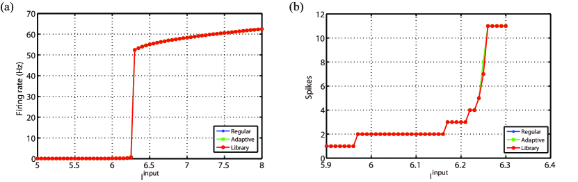
Figure 3: (a) The firing rate as a function of constant input $I^{\textrm{input}}$ ($\mu\textrm{A$\cdot$cm}^{-2}$). (b) The number of spikes during the transient period with initial voltage $V=-65$ mV. The blue and red curves in (a) and (b) indicate the regular method with $\Delta t=2^{-5}=0.03125$ ms and library method with $\Delta t=0.25$ ms, respectively.

We now further check whether the library method can still capture this Hopf phenomena in a large-scale network. We use an all-to-all connected network with 100 excitatory neurons. Each neuron is driven by a constant input $I^{\textrm{input}}$ that follows a uniform distribution with mean value around the critical value. As shown in Fig 4, the library method can still capture the spike events well, with few spikes missed because of the same coarse reason.

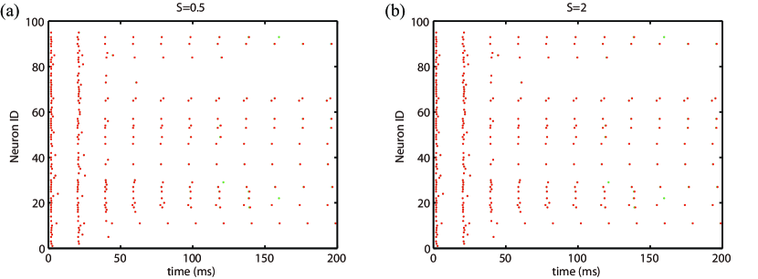
Figure 4: Raster plots of spike events in an all-to-all connected network with 100 excitatory neurons, coupling strength (a) $S=0.5$ $\textrm{mS$\cdot$cm}^{-2}$ and (b) $S=2$ $\textrm{mS$\cdot$cm}^{-2}$. Each neuron is driven by a constant input $I^{\textrm{input}}\sim U(5.9,6.3)$. Time steps and colors are the same as that in Fig 3.

3 Results

3.1 Lyapunov exponent

In this section, we show that the library method with large time steps can capture the statistical properties of the HH network. For the sake of simplicity, we show the numerical results mainly using an all-to-all connected network of 100 excitatory neurons with fixed feedforward Poisson input $\nu=100$ Hz and $f=0.10$ $\textrm{ mS$\cdot$cm}^{-2}$. Then the coupling strength $S$ is the only remaining variable. Other types of HH network and other dynamic regimes can be easily extended and similar results can be obtained.

We first study the dynamic properties of the system by computing the largest Lyapunov exponent which is one of the most important tools to characterize chaotic dynamics [19]. The spectrum of Lyapunov exponents can measure the average rate of divergence or convergence of the reference and the initially perturbed orbits [20, 21, 22]. If the largest Lyapunov exponent is positive, then the reference and perturbed orbits will exponentially diverge and the dynamics is chaotic, otherwise, the dynamics is non-chaotic.

When calculating the largest Lyapunov exponent, denoted by $\lambda$, we use $\mathbf{X}=[X_{1},X_{2},...,X_{N}]$ to represent all the variables of the neurons in the HH model. Denote the reference and perturbed trajectories by $\mathbf{X}(t)$ and $\mathbf{\tilde{X}}(t)$, respectively, then

$$\lambda=\lim_{t\rightarrow\infty}\lim_{\epsilon\rightarrow 0}\frac{1}{t}\ln\frac{||\mathbf{\tilde{X}}(t)-\mathbf{X}(t)||}{||\epsilon||}$$ (7)

where $\epsilon$ is the initial separation. However we cannot use Eq. (7) to compute $\lambda$ directly, because for a chaotic system the separation $||\mathbf{\tilde{X}}(t)-\mathbf{X}(t)||$ is unbounded as $t\rightarrow\infty$ and a numerical ill-condition will happen. The standard algorithm to compute the largest Lyapunov exponent can be found in [22, 23, 24]. The regular method can compute $\lambda$ using these algorithms directly. However, for the library method, the information of $V,m,h,n$ are blank during the stiff period and these algorithms do not work. The extended algorithm in [25] can solve this problem and we use it in this Letter.

As shown in Fig 5(a), we compute the largest Lyapunov exponent as a function of coupling strength $S$ from 0 to 2 $\textrm{mS$\cdot$cm}^{-2}$ by regular and library methods, respectively. The total run time $T$ is 60 seconds which is sufficiently long to have convergent results. The library method with a large time step $\Delta t=0.25$ ms can obtain accurate largest Lyapunov exponent compared with the regular method with a small time step $\Delta t=0.03125$ ms. The results show three typical dynamical regimes that the system is chaotic in $0.55\lesssim S\lesssim 0.875$ $\textrm{mS$\cdot$cm}^{-2}$ and non-chaotic in $0\lesssim S\lesssim 0.55$ and $0.875\lesssim S\lesssim 2$ $\textrm{mS$\cdot$cm}^{-2}$, depending on whether $\lambda$ is positive or negative.

As shown in Fig 5(b), we compute the mean firing rates, denoted by $R$, obtained by the regular and library methods to further demonstrate how accurate the library method is. We also give the relative error in the mean firing rate, which is defined by

$$E_{\textrm{R}}^{\textrm{}}=|R_{\textrm{library}}-R_{\textrm{regular}}|/R_{\textrm{regular}}$$ (8)

As shown in Fig 5(c), the library method can achieve at least 2 digits of accuracy using large time steps ($\Delta t=0.25$ ms).

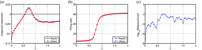
Figure 5: (a) The largest Lyapunov exponent of the HH network versus the coupling strength $S$. (b) Mean firing rate (Hz) versus the coupling strength $S$. (c) The relative error in the mean firing rate between the library and the regular method . The blue and red curves in (a) and (b) indicate the regular method with $\Delta t=2^{-5}=0.03125$ ms and library method with $\Delta t=0.25$ ms, respectively. The total run time is 60 seconds to obtain convergent results.

From the calculation of the largest Lyapunov exponent, we have known that there are three typical dynamical regimes in the HH model. As shown in Fig 6, these three regimes are asynchronous regime in $0\lesssim S\lesssim 0.55$ $\textrm{mS$\cdot$cm}^{-2}$, chaotic regime in $0.55\lesssim S\lesssim 0.875$ $\textrm{mS$\cdot$cm}^{-2}$ and synchronous regime in $0.875\lesssim S\lesssim 2$ $\textrm{mS$\cdot$cm}^{-2}$. Hence we choose three typical coupling strength $S=0.3,0.7$ and $1$ $\textrm{mS$\cdot$cm}^{-2}$ to represent these dynamical regimes, respectively, in the following numerical tests.

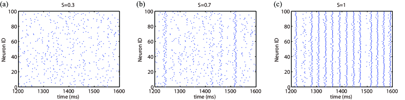
Figure 6: Raster plots of firing events in three typical dynamical regimes with coupling strength (a) $S=0.3$ $\textrm{mS$\cdot$cm}^{-2}$, (b) $S=0.7$ $\textrm{mS$\cdot$cm}^{-2}$, (c) $S=1$ $\textrm{mS$\cdot$cm}^{-2}$. Since all the three methods have similar raster, we only show the result obtained by the regular method.

3.2 The statistical accuracy of voltage

We now study the statistical accuracy of voltage. We first compute the power spectrum of the voltage trace, averaged over all the neurons, as shown in Fig 7. The library method with large time steps can capture the frequencies as well as the regular method, $i.e.$, the library method can capture the first order information of the voltage.

We should point out that when computing the power spectrum, we need the trace of voltage $V$, which is blank during the stiff period in the library method. To solve this problem, we record the trace of voltage $V(t;I^{\textrm{th}},m^{\textrm{th}},h^{\textrm{th}},n^{\textrm{th}})$ when building the library, where $I^{\textrm{th}},m^{\textrm{th}},h^{\textrm{th}},n^{\textrm{th}}$ are the corresponding initial values. In this Letter, we use sampling rate $256$ kHz to record. Then we can perform a linear interpolation to estimate the voltage during the stiff period in the library method. Note that the record process of the trace of voltage is not necessary to evolve the HH model with the library method.

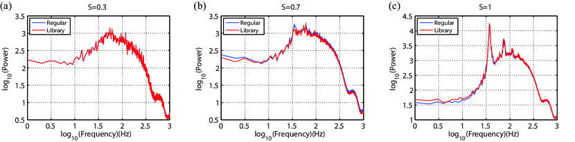
Figure 7: The averaged power spectrum of voltage trace in three typical dynamical regimes with coupling strength (a) $S=0.3$ $\textrm{mS$\cdot$cm}^{-2}$, (b) $S=0.7$ $\textrm{mS$\cdot$cm}^{-2}$, (c) $S=1$ $\textrm{mS$\cdot$cm}^{-2}$. We choose 2kHz for our sampling rate. The time steps and colors used are the same as the one in Fig 5.

We further demonstrate that the library method can capture higher order information of voltage, $e.g.$, the second and third order. Given the voltage traces of two neurons, we can compute their cross power spectral density (cpsd) and its $L^{2}$-norm. We use cpsd function in Matlab to compute in this Letter. Fig 8(a-c) show the $L^{2}$-norm of cpsd between two randomly chosen neurons with different coupling strength $S=0.3,0.7$ and $1$ $\textrm{mS$\cdot$cm}^{-2}$, while Fig 8(d-f) show the results among three neurons. Therefore, the library method with large time steps can also capture the second and third order information of voltage as well as the regular method.

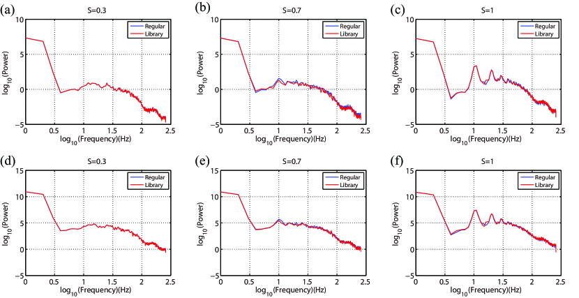
Figure 8: Top panel : The $L^{2}$-norm of cpsd between two randomly chosen neurons with coupling strength $S=0.3,0.7$ and $1$ $\textrm{mS$\cdot$cm}^{-2}$. Bottom panel : The $L^{2}$-norm of cpsd among three randomly chosen neurons with coupling strength $S=0.3,0.7$ and $1$ $\textrm{mS$\cdot$cm}^{-2}$. For example, given the traces of voltage $V_{1}(t),V_{2}(t)$ and $V_{3}(t)$, we use the information of $V_{1}(t),V_{2}(t+\tau)$ and $V_{3}(t)$ to compute cpsd. The time steps and colors used are the same as the one in Fig 5.

3.3 The statistical accuracy of spikes

Thanks to the advances in the spike train measurement like multiple electrode recording techniques, neuroscientists can obtain large amounts of spike data much easier than the voltage. The data can be used in statistical tools, $e.g.$, transfer entropy, maximum entropy and Granger causality [26, 27, 28, 5, 7]. Based on the spike trains, these tools can not only solve the directed causal information and network inference problem [4, 5] but also probe the structure of fire patterns [27, 29, 7]. Another advantage over the voltage is that the spike train data is binary, hence the state space is very small. For example, considering the vector $\mathbf{x}^{(10)}=(x_{1},x_{2},...,x_{10})$ from the spike data, the state space is only $2^{10}=1024$. So it is much easier applied to these tools while achieving faster calculation. Therefore, it is necessary to check if the library method can still obtain accurate spike trains.

As shown in Fig 5, we demonstrate the accuracy of mean firing rate by the library method. However, this is the first order information of spike trains and the at least two digits of accuracy is still very coarse. We now further demonstrate the statistical accuracy of spikes. When evolving the HH model (1), we randomly choose 10 neurons from the network, record their spike times and transform them into binary time series with a time bin 10 ms. We set the value 1 if there is a spike event during the time bin and 0 otherwise. Therefore, the 10 neurons can make up a 10-dimensional vector with total 1024 kinds of combinations. After evolving with a sufficiently long run time, we can obtain a quite accurate distribution of the 10-dimensional vector. As shown in Fig 9, we compare the probabilities of the 10-dimensional vector computed by the library and regular methods. Each star indicates the probability of the same vector (fire pattern) computed by the two methods. If the stars are on the diagonal line, then the library method can capture quite the same distribution as the regular method.

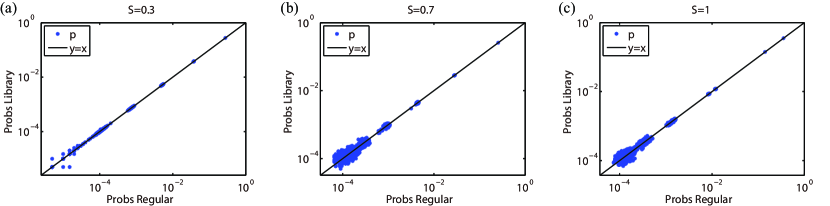
Figure 9: The comparison of the probabilities of the 10-dimesional vector by regular and library method. The stars indicate the probability of the same vector computed by two methods. Therefore, the stars on the diagonal line $y=x$ mean the probabilities are the same and the compared method is as well as the regular method. Time steps are the same as the one in Fig 5. Total run time is $10000$ seconds to obtain precise distribution.

We also do chi-square two sample tests for the comparison of distributions between the library and regular methods. The test statistic with different coupling strength all has p-value greater than $1-10^{-10}$. Therefore, the distributions from the regular and library methods cannot be distinguished in a statistical sense, $e.g.$, the library method can capture the fire patterns very well. Since the statistical tools need only the distribution of fire patterns, we can use the spike trains computed by the library method with large time steps in application.

3.4 Computational efficiency

We now demonstrate the computational efficiency of the library method by comparing the time each method costs with the same total run time. To reduce the system error from the computer, we use a sufficiently long run time of 50 seconds. In the comparison, we fix the time step $\Delta t=2^{-5}=0.03125$ ms in the regular method and change time step in the library method with a maximum value $\Delta t=0.354$ ms. As shown in Fig 10(a), the library method can overall stably obtain a maximum computational speedup around 6 times compared with the regular method. We find that the computational speedup is not increased linearly with the time step. This is because when we use a large time step, the spike-spike correction procedure requires more computation. Besides, once a neuron fires a spike, the library method should call the library for once and evolve the parameters $G$ and $H$ during the stiff period as usual which also costs some time. Therefore, the computational speedup is not increased straightforwardly with the time step.

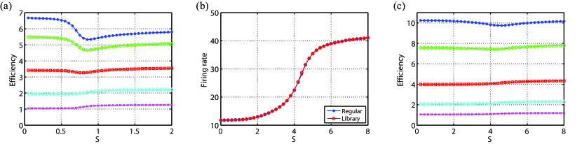
Figure 10: (a) The efficiency of the library method versus the coupling strength $S$ with the time steps $\Delta t=0.354,0.25,0.125,0.0625,0.03125$ ms from top to bottom. Total run time is 50 seconds. (b) Mean firing rate (Hz) and (c) efficiency in a sparse network with 100 excitatory neurons randomly connected with probability 15%. The coupling strength $S_{ij}=S/N$ if there is a connection from $j$-th neuron to $i$-th neuron. Other parameters and time steps are the same as that in (a)

In the all-to-all connected network, once a neuron fires a spike, all the other neurons should update their state and preliminarily evolve the HH equations (1) to find the next spike time. We should point out that real neuron networks are often sparsely connected [30, 31, 32, 33]. So only a few portion of the remaining neurons should update their state when there is a spike event. Therefore, the efficiency shown in Fig 10(a) is underestimated. We consider a sparse network with 100 excitatory neurons randomly connected with probability 15%. As shown in Fig 10(c), the library method can achieve at most 10 times of efficiency with the maximum time step $\Delta t=0.354$ ms.

3.5 Extension

3.5.1 More realistic networks

The results presented in section 3 are mainly based on an all-to-all coupled network. We now consider networks with more complicated structure, $e.g.$, let the firing rates and coupling strength of the model neurons have a distribution [31, 34] rather than a homogeneously value of $S/N$ or nearly fixed firing rate. And further check the validity of the library method in more complicated situations.

We first use a network of 100 excitatory neurons, randomly coupled with probability 15% as shown in Fig 11(a). The coupling strength of each connection follows a Uniform distribution $U(0,0.04)$ $\textrm{ mS$\cdot$cm}^{-2}$ and the Poisson input rate to each neuron follows also a Uniform distribution $U(0,200)$ Hz. Then the firing rate of each neuron has a large range from 0 to tens of Hz as shown in Fig 11(b). We check the statistical accuracy of both voltage and fire patterns in Fig 11(c-f). The test statistic of chi-square two sample tests always has $p$-value greater than $1-10^{-10}$, unless stated otherwise. The library method with a large time step $\Delta t=0.25$ ms can still achieve good performance compared with the regular method.

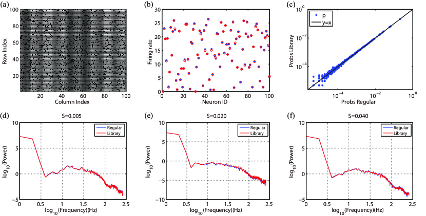
Figure 11: The performance of library method in a network of 100 excitatory neurons, randomly coupled with probability 15%. The coupling strength $S_{ij}\sim U(0,0.04)$ $\textrm{ mS$\cdot$cm}^{-2}$, the Poisson input rate $\nu_{i}\sim U(0,200)$ Hz, the Poisson input strength $f=0.1$ $\textrm{ mS$\cdot$cm}^{-2}$. The blue and red colors indicate the result from regular method with $\Delta t=2^{-5}=0.03125$ ms and library method with $\Delta t=0.25$ ms, respectively. (a) The synaptic adjacency matrix with a black color indicating a connection and white color otherwise. (b) Firing rate of each neuron. (c) The comparison of the probabilities of the 10-dimesional vector. The $L^{2}$-norm of cpsd between two neurons with different coupling strength (d) $S=0.005$ $\textrm{ mS$\cdot$cm}^{-2}$, (e) $S=0.020$ $\textrm{ mS$\cdot$cm}^{-2}$, (f) $S=0.040$ $\textrm{ mS$\cdot$cm}^{-2}$

According to data from living cortical neuronal networks, the coupling strength follows a Log-normal distribution [31]. We then adjust the coupling strength following from a Uniform distribution to a Log-normal distribution but keep the mean value of 0.02 $\textrm{ mS$\cdot$cm}^{-2}$. As shown in Fig 12, the library method can still achieve good performance.

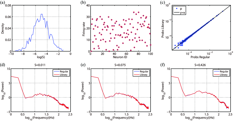
Figure 12: The performance of library method in the same network as shown in Fig 11 but with coupling strength $S_{ij}\sim\textrm{Lognormal}(-4.890,1.956)$ $\textrm{ mS$\cdot$cm}^{-2}$ (the mean value of $S_{ij}=0.02$ $\textrm{ mS$\cdot$cm}^{-2}$). The colors and time steps are the same as that in Fig 11. (a) The distribution of the coupling strength. (b) Firing rate of each neuron. (c) The comparison of the probabilities of the 10-dimesional vector. The $L^{2}$-norm of cpsd between two neurons with different coupling strength (d) $S=0.011$ $\textrm{ mS$\cdot$cm}^{-2}$, (e) $S=0.075$ $\textrm{ mS$\cdot$cm}^{-2}$, (f) $S=0.426$ $\textrm{ mS$\cdot$cm}^{-2}$.

3.5.2 Extended HH-type models

In this part, we apply the library method to other types of HH model for the four most prominent classes of neurons. They are “regular spiking” (RS), “fast spiking” (FS), “intrinsically bursting” (IB) and “low-threshold spike” (LTS) cells according to the pattern of spiking and bursting in intracellular recordings [35]. These HH-type models are obtained by fit method based on different experimental data like from rat somatosensory cortex in vitro, ferret visual cortex in vitro, cat visual cortex in vivo and cat association cortex in vivo. All the four extended HH-type models can be described by the following equation [12]:

$$C_{m}\frac{dV_{i}}{dt}=-g_{\textrm{leak}}(V_{i}-E_{\textrm{leak}})-I_{i}^{\textrm{Na}}-I_{i}^{\textrm{Kd}}-I_{i}^{\textrm{M}}-I_{i}^{\textrm{T}}-I_{i}^{\textrm{L}}+I_{i}^{\textrm{input}}$$ (9)

where $V_{i}$ is the membrane potential of the $i$-th neuron, $I_{i}^{\textrm{Na}},I_{i}^{\textrm{Kd}},I_{i}^{\textrm{M}},I_{i}^{\textrm{T}}$ and $I_{i}^{\textrm{L}}$ are voltage-dependent currents, $I_{i}^{\textrm{input}}$ is the input current, $C_{m}=1\mu\textrm{F$\cdot$c$m^{-2}$}$ is the specific capacitance of the membrane, $g_{\textrm{leak}}$ and $E_{\textrm{leak}}$ are the resting membrane conductance and reversal potential, respectively. Detailed functions and parameters for the four extended HH-type models [12] are given in Appendix.

RS neurons are the most typical neurons in neocortex and is in general excitatory. When injected by a constant depolarizing current, the neurons can fire with short inter-spike-interval (ISI) at first and then the ISI increases and tends to be stable as shown in Fig 13(a). This is called spike-frequency adaptation which is one of the mean features. We also use an excitatory RS-type network with coupling strength following a Log-normal distribution, Poisson input rate following a Uniform distribution to illustrate the validity of library method. The statistical accuracy of spikes are given in Fig 13(e, i).

We should point out that the extended HH-type model contains more voltage-dependent currents, $e.g.$, the IB-type model requires 7 parameters: $I^{\textrm{th}},m^{\textrm{th}},h^{\textrm{th}},n^{\textrm{th}},p^{\textrm{th}},q^{\textrm{th}},r^{\textrm{th}}$ when building the library. As a consequence, the trace of voltage during the stiff period will occupy huge storage space (>10 gigabyte in binary form). Therefore, we do not record the trace of voltage when building the library and present the accuracy of voltage.

FS neurons are another kind of typical neurons in cortex and is in general inhibitory. The mean feature of a FS neuron is that it can fire high-frequency spikes with little or no adaptation, as shown in Fig 13(b). We use an inhibitory FS-type network to show the validity of library method in Fig 13(f, j).

IB neurons are usually excitatory and can produce bursts of spikes, while LTS neurons are usually inhibitory and can fire high-frequency spikes with spike-frequency adaptation. The validity of library method for the IB and LTS network are given in the third and last column of Fig 13, respectively.

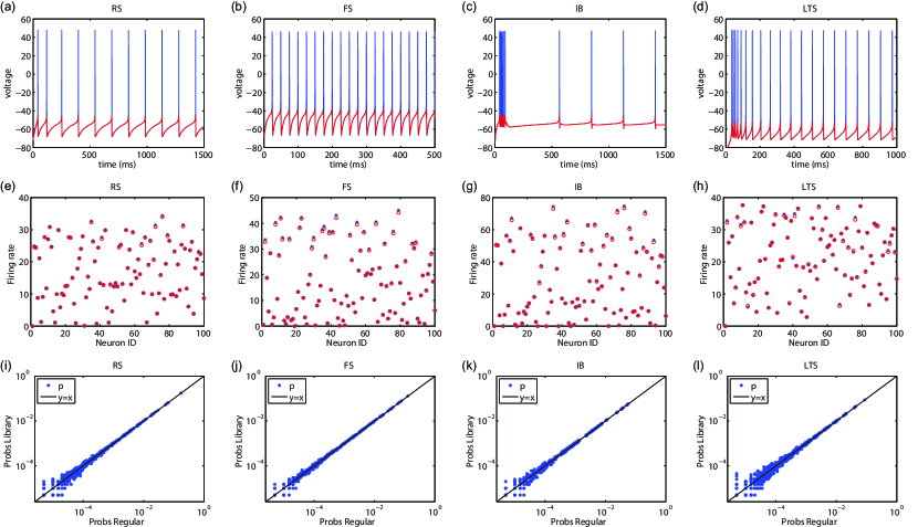
Figure 13: The validity of library method for the extended HH-type models. Top panel: Voltage traces of a single neuron driven by a constant input. Constant input are $I^{\textrm{input}}=0.8,4,0.4,2.2$ $\mu\textrm{A$\cdot$cm}^{-2}$ for the RS, FS, IB and LTS neurons, respectively. Middle panel: Firing rate of each neuron of the RS, FS, IB and LTS networks. Bottom panel: The comparison of the probabilities of the 10-dimesional vector for the RS, FS, IB and LTS networks. The colors and time steps are the same as that in Fig 11. All the four networks have 100 neurons (RS and IB are excitatory network while FS and LTS are inhibitory network), coupled as in Fig 11(a), Poisson input strength $f=0.1$ $\textrm{ mS$\cdot$cm}^{-2}$. Other parameters are RS: coupling strength $S_{ij}\sim\textrm{Lognormal}(-5.757,2.303)$, Poisson input rate $\nu_{i}\sim U(0,200)$ Hz; FS: $S_{ij}\sim\textrm{Lognormal}(-5.757,2.303)$, $\nu_{i}\sim U(200,600)$ Hz; IB: $S_{ij}\sim\textrm{Lognormal}(-6.623,2.649)$, $\nu_{i}\sim U(0,100)$ Hz; LTS: $S_{ij}\sim\textrm{Lognormal}(-5.757,2.303)$, $\nu_{i}\sim U(0,400)$ Hz.

4 Conclusion

In conclusion, we have shown a modified library method to deal with the stiff part during the firing event in evolving the HH model. The library method can enlarge time step (maximum time step 0.354 ms) to reduce the computational cost while achieving high accurate statistical information of the HH neurons. It is worthwhile pointing out that the library method with large time steps can capture the fire patterns or the distribution of the spikes as well as the regular method. This holds a spectral attraction to apply to statistical analysis like the transfer entropy and maximum entropy which require a sufficiently long run time $\sim 20$ minutes to obtain a precise distribution of spikes. However, due to the extra error introduced by calling the library, it can never obtain numerical convergence. But the library method can still retain most of the properties of HH neurons like the chaotic dynamics which is observed in the HH model by computing the largest Lyapunov exponent.

We emphasize that the library method is very attractive with a stably maximum 10 times of speedup in a sparse network. The remarkable speedup of library method holds in spite of the size of the network or the structure of connectivity.

We can successfully extend the idea of library method in more complicated HH-type models with bursting and adaptation behavior. The way to build and use the library are the same as that in the standard HH model although there are more voltage-dependent currents. The library method can also capture most of the statistical properties of these HH-type neurons with high times of speedup.

Finally, we emphasize that the spike-spike correction procedure [10] is necessary in the two methods, especially using a large time step in the library method. This procedure ensures that the spiking sequences estimated are accurate. Even in a strongly coupled network, the synaptic interactions are still correct and will not influence the accuracy of the library method.

References

- [1] Alan L Hodgkin and Andrew F Huxley. A quantitative description of membrane current and its application to conduction and excitation in nerve. The Journal of physiology, 117(4):500, 1952.
- [2] Brian Hassard. Bifurcation of periodic solutions of the hodgkin-huxley model for the squid giant axon. Journal of Theoretical Biology, 71(3):401–420, 1978.
- [3] Peter Dayan and LF Abbott. Theoretical neuroscience: computational and mathematical modeling of neural systems. Journal of Cognitive Neuroscience, 15(1):154–155, 2003.
- [4] Shinya Ito, Michael E Hansen, Randy Heiland, Andrew Lumsdaine, Alan M Litke, and John M Beggs. Extending transfer entropy improves identification of effective connectivity in a spiking cortical network model. PloS one, 6(11):e27431, 2011.
- [5] Douglas Zhou, Yanyang Xiao, Yaoyu Zhang, Zhiqin Xu, and David Cai. Granger causality network reconstruction of conductance-based integrate-and-fire neuronal systems. PloS one, 9(2):e87636, 2014.
- [6] Douglas Zhou, Yanyang Xiao, Yaoyu Zhang, Zhiqin Xu, and David Cai. Causal and structural connectivity of pulse-coupled nonlinear networks. Physical review letters, 111(5):054102, 2013.
- [7] Zhi-Qin John Xu, Guoqiang Bi, Douglas Zhou, and David Cai. A dynamical state underlying the second order maximum entropy principle in neuronal networks. Communications in Mathematical Sciences, 15(3):665–692, 2017.
- [8] David Hansel, Germán Mato, Claude Meunier, and L Neltner. On numerical simulations of integrate-and-fire neural networks. Neural Computation, 10(2):467–483, 1998.
- [9] Michael J Shelley and Louis Tao. Efficient and accurate time-stepping schemes for integrate-and-fire neuronal networks. Journal of Computational Neuroscience, 11(2):111–119, 2001.
- [10] Aaditya V Rangan and David Cai. Fast numerical methods for simulating large-scale integrate-and-fire neuronal networks. Journal of Computational Neuroscience, 22(1):81–100, 2007.
- [11] Eugene M Izhikevich. Simple model of spiking neurons. IEEE Transactions on neural networks, 14(6):1569–1572, 2003.
- [12] Martin Pospischil, Maria Toledo-Rodriguez, Cyril Monier, Zuzanna Piwkowska, Thierry Bal, Yves Frégnac, Henry Markram, and Alain Destexhe. Minimal hodgkin–huxley type models for different classes of cortical and thalamic neurons. Biological cybernetics, 99(4):427–441, 2008.
- [13] Maurizio Mattia and Paolo Del Giudice. Efficient event-driven simulation of large networks of spiking neurons and dynamical synapses. Neural Computation, 12(10):2305–2329, 2000.
- [14] Jan Reutimann, Michele Giugliano, and Stefano Fusi. Event-driven simulation of spiking neurons with stochastic dynamics. Neural Computation, 15(4):811–830, 2003.
- [15] Michelle Rudolph and Alain Destexhe. How much can we trust neural simulation strategies? Neurocomputing, 70(10):1966–1969, 2007.
- [16] Yi Sun, Douglas Zhou, Aaditya V Rangan, and David Cai. Library-based numerical reduction of the hodgkin–huxley neuron for network simulation. Journal of computational neuroscience, 27(3):369–390, 2009.
- [17] Wulfram Gerstner and Werner M Kistler. Spiking neuron models: Single neurons, populations, plasticity. Cambridge university press, 2002.
- [18] Christof Koch and Idan Segev. Methods in neuronal modeling: from ions to networks. MIT press, 1998.
- [19] Valery Iustinovich Oseledec. A multiplicative ergodic theorem. lyapunov characteristic numbers for dynamical systems. Trans. Moscow Math. Soc, 19(2):197–231, 1968.
- [20] Edward Ott. Chaos in dynamical systems. Cambridge university press, 2002.
- [21] John Michael Tutill Thompson and H Bruce Stewart. Nonlinear dynamics and chaos. John Wiley & Sons, 2002.
- [22] Thomas S Parker and Leon Chua. Practical numerical algorithms for chaotic systems. Springer Science & Business Media, 2012.
- [23] Douglas Zhou, Yi Sun, Aaditya V Rangan, and David Cai. Spectrum of lyapunov exponents of non-smooth dynamical systems of integrate-and-fire type. Journal of computational neuroscience, 28(2):229–245, 2010.
- [24] Alan Wolf, Jack B Swift, Harry L Swinney, and John A Vastano. Determining lyapunov exponents from a time series. Physica D: Nonlinear Phenomena, 16(3):285–317, 1985.
- [25] Douglas Zhou, Aaditya V Rangan, Yi Sun, and David Cai. Network-induced chaos in integrate-and-fire neuronal ensembles. Physical Review E, 80(3):031918, 2009.
- [26] Donald H Perkel, George L Gerstein, and George P Moore. Neuronal spike trains and stochastic point processes: Ii. simultaneous spike trains. Biophysical journal, 7(4):419–440, 1967.
- [27] Jonathon Shlens, Greg D Field, Jeffrey L Gauthier, Matthew I Grivich, Dumitru Petrusca, Alexander Sher, Alan M Litke, and EJ Chichilnisky. The structure of multi-neuron firing patterns in primate retina. Journal of Neuroscience, 26(32):8254–8266, 2006.
- [28] Christopher J Quinn, Todd P Coleman, Negar Kiyavash, and Nicholas G Hatsopoulos. Estimating the directed information to infer causal relationships in ensemble neural spike train recordings. Journal of computational neuroscience, 30(1):17–44, 2011.
- [29] Jonathon Shlens, Greg D Field, Jeffrey L Gauthier, Martin Greschner, Alexander Sher, Alan M Litke, and EJ Chichilnisky. The structure of large-scale synchronized firing in primate retina. Journal of Neuroscience, 29(15):5022–5031, 2009.
- [30] David Golomb and David Hansel. The number of synaptic inputs and the synchrony of large, sparse neuronal networks. Neural computation, 12(5):1095–1139, 2000.
- [31] Sen Song, Per Jesper Sjöström, Markus Reigl, Sacha Nelson, and Dmitri B Chklovskii. Highly nonrandom features of synaptic connectivity in local cortical circuits. PLoS biology, 3(3):e68, 2005.
- [32] Christopher J Honey, Rolf Kötter, Michael Breakspear, and Olaf Sporns. Network structure of cerebral cortex shapes functional connectivity on multiple time scales. Proceedings of the National Academy of Sciences, 104(24):10240–10245, 2007.
- [33] Wulfram Gerstner, Werner M Kistler, Richard Naud, and Liam Paninski. Neuronal dynamics: From single neurons to networks and models of cognition. Cambridge University Press, 2014.
- [34] Tomáš Hromádka, Michael R DeWeese, and Anthony M Zador. Sparse representation of sounds in the unanesthetized auditory cortex. PLoS biology, 6(1):e16, 2008.
- [35] Barry W Connors and Michael J Gutnick. Intrinsic firing patterns of diverse neocortical neurons. Trends in neurosciences, 13(3):99–104, 1990.