Query-Based Selection of Optimal Candidates under the Mallows Model

Abstract

We study the secretary problem in which rank-ordered lists are generated by the Mallows model and the goal is to identify the highest-ranked candidate through a sequential interview process which does not allow rejected candidates to be revisited. The main difference between our formulation and existing models is that, during the selection process, we are given a fixed number of opportunities to query an infallible expert whether the current candidate is the highest-ranked or not. If the response is positive, the selection process terminates, otherwise, the search continues until a new potentially optimal candidate is identified. Our optimal interview strategy, as well as the expected number of candidates interviewed and the expected number of queries used, can be determined through the evaluation of well-defined recurrence relations. Specifically, if we are allowed to query $s-1$ times and to make a final selection without querying (thus, making $s$ selections in total) then the optimum scheme is characterized by $s$ thresholds that depend on the parameter $\theta$ of the Mallows distribution but are independent on the maximum number of queries.

1 Introduction

The secretary problem, also known as the game of googol and the picky bride problem, was formally introduced by Gardner [11, 12] and is considered a prototypical example in sequential analysis, optimization, and decision theory. It can be stated as follows: $N$ individuals are assumed to be ranked from best-to-worst without ties according to their qualifications. They apply for a “secretary” position, and are interviewed one by one, in a uniformly random order. When the $i^{\text{th}}$ candidate appears, one can only rank her/him with respect to the $i-1$ already interviewed individuals. At the time of the $i^{\text{th}}$ interview, the employer can make the decision to hire the person presented or continue with the interview process by rejecting the candidate; rejected candidates cannot be revisited at a later time. If only one selection is to be made, what selection strategy (i.e., stopping rule) maximizes the probability of selecting the best (highest ranked) candidate?

The first published solution to the problem is due to Lindley [19] in 1961 and is based on algebraic methods. Dynkin [5] solved the problem in 1963 by viewing the selection process as a Markov chain. For $N$ large enough, the answer turns out to be surprisingly elegant and simple: the first $N/e$ candidates are automatically rejected ($e$ stands for the base of the natural logarithm) and the first candidate that outranks all previously seen candidates after that point is selected for an offer. This strategy ensures a probability of successful identification of the best candidate equal to $1/e$, provided that $N$ is allowed to go to infinity.

The secretary problem has been extended in many directions. Examples include full information games [15], the classical secretary problem on posets [9, 13, 14, 24] and in the context of matroid theory [2, 26], as well as the Prophet inequality model [18]. For more extensions and a detailed history of the development of secretary problem, the interested reader is referred to [6, 8]. In particular, an extension of the classical secretary problem, known as the Dowry problem with multiple choices (henceforth, the Dowry problem), was studied by Gilbert and Mosteller in their seminal work [15]. In the Dowry problem, one is allowed to select $s\geq 1$ candidates during the interview process, and the criteria for success is that the selected group includes the optimal candidate. This review process can be motivated or extended in many different ways: For example, one may view the $s$-collection to represent candidates invited for a second round of interviews.

For both the secretary and Dowry problem, the modeling assumption is that the candidates are presented to the evaluator uniformly at random. Nevertheless, it is often the case that the candidates are presented in an order that is nonuniform [4, 16, 17, 20, 21]. This consideration lends itself to a generalization of the secretary problem introduced by Jones in [17]. The paper [17] considers candidates arriving in an order dictated by a sample permutation from the Mallows distribution [22]. In particular, when $N\to\infty$, Jones [17] showed that the optimal strategy for the classical secretary problem under the Mallows model (parametrized by $\theta>0$) is as follows: (1) when $\theta<1$, reject all but the last $j=\max(-1/\ln{\theta},1)$ candidates and select the next left-to-right maximum thereafter; and (2) when $\theta>1$, reject the first $k$ candidates and select the next left-to-right maximum thereafter. Here, $k$ is a function of $\theta$ but independent on $N$. It is important to point out that the focus of the work addressed the secretary problem (with one selection), with recent extensions providing companion solutions for the postdoc problem [20, 21], introduced by Dynkin in the 1980s [25, 27].

Motivated by a recent line of problems considering learning problems with queries [1, 3, 10, 23], we introduce the problem of query-based sequential analysis under the Mallows model. In our setting, we make use of the Mallows distribution and assume that the decision making entity has access to a limited number of queries to an infallible expert. When faced with a candidate identified by an exploration-exploitation procedure as the potentially optimal choice, an expert provides an answer of the form “Best” and “Not the best.” If the answer is “Not the best,” a new exploration-exploitation stage is initiated, with the potential of using another query at the end of the process. If the answer is “Best,” the sequential examination process terminates. Given a budget of $s-1$ queries, where $s$ is usually a relatively small positive integer, e.g., $2\leq s\leq 5$, the questions of interest is to find the optimal interview strategy, the optimal probability of success and the expected number of candidates interviewed or experts queried until success or termination. Note that we are allowed to make a final selection without querying experts after using all $s-1$ queries; thus, we have a budget of $s-1$ queries and can make at most s selections.

When applied on the random interview model, the above setting resembles the Dowry problem as both allow for selecting $s$ candidates. In the Dowry problem, one is allowed to make $s$ selections without the information about the global ranking of the selected candidates while in our query-based setting the expert is asked if the candidate is globally the best. Furthermore, it assumes that candidate lists are Mallows samples and even for the Dowry problem, such a distribution assumption was not considered in the past.

For a Mallows distribution parametrized by $\theta>0$, the case $\theta>1$ corresponds to a decreasing trend in the quality of candidates while the case $0<\theta<1$ corresponds to an increasing trend in the quality of candidates. The case $\theta=1$ corresponds to the uniform distribution. In our query-based model, we are provided with $s-1$ ($s\geq 1$) opportunities to query an expert whether the current candidate is the best or not. If the best candidate is not identified after these queries we are still allowed to make a final selection without querying experts. In terms of the optimal probability of winning and the optimal strategy, the query-based model with $s-1$ queries is equivalent to the Dowry problem with $s$ selections, since (i) they both have in total a maximum budget of $s$ selections; (ii.1) if a selected candidate presented as the $i^{\text{th}}$ selection, where $1\leq i\leq s-1$, is the globally best candidate then in the query-based model we accept this candidate and stop our search. In the Dowry model we select, save, and move on since we still have at least one selection left, which will not influence the result as we already picked the best candidate; (ii.2) if the $s^{\text{th}}$ selection is the best candidate, the two models are equivalent as we will save the selected candidate in both models; (iii.1) if a candidate at the $i^{\text{th}}$ selection time, where $1\leq i\leq s-1$, is not the globally best candidate then in the query-based model we will be informed about this fact and will continue the search while in the Dowry model we will not have this information available but will still continue since there is at least one selection left; (iii.2) if a selected candidate at the $s^{\text{th}}$ selection point is not the best, then under both models we will save the candidate and terminate.

The optimal query and selection strategies for both our query-based model and the Dowry model depend on the value of the parameter $\theta$ of the Mallows model. For $N\to\infty$ and $\theta>1$, the optimal strategy is an $s$-threshold $(k_{1},\ldots,k_{s})$-strategy (formally defined in Theorem 25) with $0\leq k_{1}\leq\ldots\leq k_{s}\not\to\infty$, where $k_{i}$, $1\leq i\leq s$, is the threshold for the $i^{\text{th}}$ selection. In this setting, an optimal strategy is as follows: When making the $i^{\text{th}}$ selection, for each $1\leq i\leq s$, we reject all candidates up until position $k_{i}$, then select the next left-to-right maxima (a candidate which is the best when compared with all examined candidates up to that point). For $0<\theta<1$, the optimal strategy is also an $s$-threshold $(k_{1},\ldots,k_{s})$-strategy; however, in this case, $k_{1}\leq\ldots\leq k_{s}\leq N-1$ and $N-k_{1}\not\to\infty$.

Furthermore, let $N$ be a fixed positive integer; for each positive real number $\theta$, there exists a sequence of numbers $a_{1}(\theta),a_{2}(\theta),\ldots$ that depends only on $\theta$, such that $a_{1}(\theta)\geq a_{2}(\theta)\geq a_{3}(\theta)\geq\ldots$ and an optimal strategy for the proposed query-based model (with $s-1$ queries in total) is the $s$-threshold $(a_{s}(\theta),\ldots,a_{1}(\theta))$-strategy. In addition, the thresholds in the $(a_{s}(\theta),\ldots,a_{1}(\theta))$-strategy do not change with the value of $s$ if read from the right. For example, let $\theta>0$ be fixed, and assume that the optimal strategy for $s=2$ is the $(a_{2}(\theta),a_{1}(\theta))$-strategy and an optimal strategy for $s=3$ is the $(a_{3}(\theta),a_{2}(\theta),a_{1}(\theta))$-strategy; when $s$ increases from $2$ to $3$, our optimal strategy will only add $a_{3}(\theta)$ on the left and the parameter values at later positions in the strategy will not change with $s$. Even though a special case of our version of the problem exhibits similarities with the Dowry problem with multiple choices proposed by Gilbert and Mosteller [15], there are essential structural and methodological differences, since in our case we allow for early stopping, address non-uniform (e.g., Mallows) candidate interview distributions and, most importantly, provide an exact (non-asymptotic) proof of the optimality of our scheme for any number of queries.

An important combinatorial method to study sequential problems under nonuniform ranking models was developed in a series of papers by Fowlkes and Jones [7], and Jones [16, 17]. For consistency, we use some of the notation and definitions from Jones [17] but also introduce a number of new concepts and combinatorial proof techniques. In particular, finding recurrence relations for more than one selection is significantly more challenging than for the secretary problem, and the optimal strategies differ substantially from the classical ones as our results include multiple thresholds for stopping.

The paper is organized as follows. Section 2 introduces the relevant concepts, terminology and models used throughout the paper. The same section also contains a number of technical lemmas that help in establishing our main results pertaining to the optimal selection strategies. An in-depth analysis of the exploration stages and the probabilities of success for the optimal selection processes under the Mallows distribution are presented in Section 4. Numerical results for the exploration phase lengths and optimal winning probabilities versus $\theta$ are discussed in Section 5. Results of our analysis for the expected number of questions (selections) used as well as the numerical results are presented in Section 6.

2 Preliminaries

The sample space is the set of all permutations of $N$ elements, i.e. the symmetric group $S_{N}$, with the underlying $\sigma$-algebra equal to the power set of $S_{N}$. The best candidate is indexed by $N$, the second-best candidate by $N-1,\ldots,$ and the worst candidate is indexed by $1$. The interview committee can accurately compare the candidates presented up to a certain time point, but cannot assess the quality of the future candidates. We also assume that there is a budget of $s-1$ queries ($s\geq 1$) to be made that produce an answer whether a current candidate is the globally best one or not, as well as a final selection that does not involved queries (thus, a total of $s$ selections). These modeling assumptins are equivalent to those of the Dowry problem with $s$ selections if one only considers the optimal probability of success and winning strategy. Still, there are differences in the expected interview times which are discussed in Section 6.

Furthermore, unlike the standard model of the secretary and Dowry problem, our framework assumes that the candidates are presented (one-by-one, from the left) according to a permutation (order) dictated by the Mallows distribution $\mathcal{M}_{\theta}$, parametrized by a real number $\theta>0$. The probability of presenting a permutation $\pi\in S_{N}$ to the hiring committee equals

$$f(\pi)=\theta^{c(\pi)}\bigg{/}\sum\limits_{\pi\in S_{N}}\theta^{c(\pi)},$$

where $c:S_{N}\to\mathbb{N}$ equals the smallest number of adjacent transpositions needed to transform $\pi$ into the identity permutation $[12\,\cdots\,N]$. Equivalently, $c(\pi)$ equals the number of pairwise element inversions, and is also known as the Kendall $\tau$ distance between the permutation $\pi$ and the identity permutation $[12\,\cdots\,N]$. Note that the notation for a permutation in square bracket form should not be confused with the notation for a set $[a,b]=\{{a,a+1,\ldots,b\}},\,b\geq a,$ and the meaning of the notation used will be clear from the context.

As remarked upon in Section 1, the query-based model and the Dowry model in the uniform permutation selection setting are the same problem when considering the maximum probability of winning and a corresponding optimal strategy. Therefore, for simplicity, we present our results for the new Mallows model in the “language” of the Dowry problem with $s$ selections.

2.1 The $Q,Q^{o},\bar{Q}$ probabilities and strike sets

For a given permutation $\pi\in S_{N}$ drawn according to the Mallows model, we say that a strategy wins if it correctly identifies the best candidate when presented with $\pi$. The notion of a prefix is introduced to represent the current relative ordering of candidates. Given a permutation $\pi\in S_{N}$, the $k^{(th)}$ prefix of $\pi$, denoted by $\pi|_{k},$ is a permutation in $S_{k}$ and it represents the relabelling of the first $k$ elements of $\pi$ according to their relative order. For example, if $\pi=[635124]\in S_{6}$ and $k=4$, then $\pi|_{4}=[4231]$.

Definition 1.

Let $\sigma\in\bigcup\limits_{i=1}^{N}S_{i}$ and assume that the length of the permutation, $|\sigma|$, equals $k$.

(1) We say that $\pi\in S_{N}$ is $\sigma$-prefixed if $\pi|_{k}=\sigma$. For example, $\pi=[165243]\in S_{6}$ is $\sigma=[1432]$-prefixed.

(2) Given that $\pi$ is $\sigma$-prefixed, we say that $\pi$ is $\sigma$-winnable if accepting the prefix $\sigma$, i.e. if accepting the $|\sigma|^{\text{th}}$ candidate when the order $\sigma$ is encountered identifies the best candidate of the interview order $\pi$. More precisely, for $\sigma=[\sigma(1)\sigma(2)\cdots\sigma(k)]$, we have that $\pi$ is $\sigma$-winnable if $\pi$ is $\sigma$-prefixed and $\pi(k)=N$.

Definition 2.

A left-to-right maxima in a permutation $\pi\in S_{N}$ is a position whose value is larger than all values to the left of the position. For example, if $\pi=[423516]\in S_{6}$, then the first, fourth, and sixth position are left-to-right maxima.

Definition 3.

We say that a permutation $\sigma\in\bigcup\limits_{i=1}^{N}S_{i}$ is eligible if it ends in a left-to-right maxima or has length $N$. For example, let $N=6$. Then both $[1324]$ and $[165243]$ are eligible.

A permutation $\pi\in S_{N}$ is sampled from the Mallows model before the interview process. During the interview process, each entry of $\pi$ is presented one-by-one from the left; the relative ordering of the positions presented so far forms a prefix of $\pi$. That is the only information that can be used to decide whether to accept or reject the current candidate. Therefore, every strategy can be represented as a set of permutations of possibly different lengths that lead to an accept decision for the last candidate observed; such a set is called a strike set. More precisely, the selection process proceeds as follow: If the prefix we have seen so far is in the strike set, then we accept the current candidate and continue (if there is at least one selection left); if it does not belong to the strike set, we reject the current candidate and continue. For example, let $N=4$ and $s=1$. Then, the boxed set of permutations $A=\{[12],[213],[3124],[3214]\}$ in Figure 1 is a strike set. The corresponding interview strategy may be summarized as follows: If the relative order of the candidates interviewed so far is in the set $A$, then accept the current candidate; otherwise, reject the current candidate.

Since in our model there are $s$ selections, we make use of $s$-strike sets defined below.

Definition 4.

A set $X\subseteq\bigcup_{j=1}^{N}S_{j}$ is called an $s$-minimal set if it is impossible to have $s+1$ elements $\alpha_{1},\alpha_{2},\ldots,\alpha_{s+1}\in X$ such that $\alpha_{i+1}$ is a prefix of $\alpha_{i}$, for all $i\in\{1,2,\ldots,s\}$.

Definition 5.

A set of permutations $A\subseteq\bigcup_{j=1}^{N}S_{j}$ is called an $s$-strike set if it satisfies the following three conditions:

(1) It comprises prefixes that are eligible.

(2) The set $A$ is $s$-minimal. The set $A$ may contain elements $\alpha_{1},\alpha_{2},\ldots,\alpha_{s}$ such that $\alpha_{i+1}$ is a prefix of $\alpha_{i}$, for all $i\in\{1,2,\ldots,s-1\}$. In other words, based on an $s$-strike set one can make at most $s$ selections.

(3) Every permutation in $S_{N}$ contains some element of $A$ as its prefix (i.e., given an $s$-strike set one can always make a selection based on its elements).

A $1$-strike set corresponds to the valid strike set defined in the paper of Jones [17] when only one choice is allowed. We use the term strike set whenever $s$, the number of total selections, is clear from the context.

From the previous definition and the fact that we are allowed to make at most $s$ selections it follows that any optimal strategy for our problem can be represented by an $s$-strike set. For example, the set {[1], [12], [213], [3124], [3214]} in Figure 1 is a $2$-strike set, which also represents an optimal strategy for the case $N=4$ and $s=2$. See also Example 27. Furthermore, for a permutation $\sigma$ of length $k$, where $1\leq k\leq N$, and $i\in\{1,2,\ldots,s\}$, we make extensive use of the following probabilities.

Definition 6.

Let $\sigma$ be a permutation of length $k$, where $1\leq k\leq N$, and let $i\in\{1,2,\ldots,s\}$. Define

$Q_{i}(\sigma)$, the probability of identifying the best candidate with the strategy accepting the $k^{\text{th}}$ position and using the best strategy thereafter conditioned on the pre-selected interviewing order $\pi$ being $\sigma$-prefixed and $i$ selections still being available when interviewing the candidate at position $k$.

$Q_{i}^{o}(\sigma)$, the probability of identifying the best candidate with the best strategy after making a decision for the $k^{\text{th}}$ position conditioned on the pre-selected interviewing order $\pi$ being $\sigma$-prefixed and $i$ selections still being available right after the interview of the $k^{\text{th}}$ candidate.

$\bar{Q}_{i}(\sigma)$, which equals $\bar{Q}_{i}(\sigma)=\max\{Q_{i}(\sigma),Q^{o}_{i}(\sigma)\}.$

In words, $Q$ represents the probability of winning by accepting the current candidate while $Q^{o}$ is the probability of winning based on future selections in the interview process. In order to ensure the maximum probability of winning, an optimal strategy will examine two available choices, i.e. “accept the current candidate” or “reject the current candidate and implement the best strategy in the future” at each stage of the interview and select the one with a better chance of identifying the best candidate.

Remark 7.

Let $1\leq i\leq s$. Consider an arbitrary permutation $\sigma$ of length $N$. If the last position of $\sigma$ is $N$, then $Q_{i}(\sigma)=1$, $Q^{o}_{i}(\sigma)=0$, and $\bar{Q}^{o}_{i}(\sigma)=1$. If the last position of $\sigma$ is not $N$, then $Q_{i}(\sigma)=0$, $Q^{o}_{i}(\sigma)=0$, and $\bar{Q}^{o}_{i}(\sigma)=0$, since selecting the last candidate will not result in success and the search will terminate after interviewing the last candidate. For a permutation $\sigma$ of length at least $N-i$, $Q_{i+1}(\sigma)=\ldots=Q_{s}(\sigma)$. Furthermore, for a permutation $\sigma$ of length at least $N-i$, $Q^{o}_{i}(\sigma)=Q_{i}^{o}(\sigma)=\ldots=Q_{s}^{o}(\sigma)$.

We also need the following definitions.

Definition 8.

Let $\sigma$ be a permutation of length $k\leq N$. The standard denominator $SD(\sigma)$ of $\sigma$ equals

$$SD(\sigma)=\sum\limits_{\sigma\text{-prefixed }\pi\in S_{N}}\theta^{c(\pi)}.$$

Furthermore, $\text{Win}(\sigma)$ stands for the sum of the weights $\theta^{c(\pi)}$ over all $\sigma$-winnable permutations $\pi\in S_{N}$.

The case $i=1$ was first analyzed by Jones [17], establishing that

$$Q_{1}(\sigma)=\frac{\sum\limits_{\sigma\text{-winnable }\pi\in S_{N}}\theta^{c(\pi)}}{\sum\limits_{\sigma\text{-prefixed }\pi\in S_{N}}\theta^{c(\pi)}}=\frac{Win(\sigma)}{SD(\sigma)}.$$ (1)

Definition 9.

The $\oplus$ operation for two fractions $\frac{a}{b}$ and $\frac{c}{d}$ is defined as $\frac{a}{b}\oplus\frac{c}{d}=\frac{a+c}{b+d}$.

Roughly speaking, the $\oplus$ operation will be used to compute the probability of the union of two disjoint events from two disjoint sample spaces over a new sample space equal to the union of the sample spaces. It is important to point out that we do not cancel common divisors in the defining fractions for the probabilities $Q,Q^{o},\bar{Q}$ until the final step.

Each entry of pre-selected permutation $\pi$ is presented one-by-one from the left during the interview process, and the relative ordering of the already observed positions forms a prefix of $\pi$. This relative ordering changes with more candidates being interviewed and we need a means to describe this process.

Definition 10.

For each $\sigma$ of length $\ell-1$, where $\ell\leq N$, we define $\lambda_{j}(\sigma)$, $1\leq j\leq\ell$, to be the $\sigma$-prefixed permutation of length $\ell$ such that its last position has value $j$; the permutation is obtained by relabelling the $\ell$ positions of $\sigma$. For example, for $\sigma=[123],$ a permutation of length $3$, we have $\lambda_{1}(\sigma)=[2341],\lambda_{2}(\sigma)=[1342],\lambda_{3}(\sigma)=[1243]$ and $\lambda_{4}(\sigma)=[1234]$.

Let $\sigma$ be a permutation of length $1\leq k\leq N$ with $Q_{i}(\sigma),Q^{o}_{i}(\sigma),\bar{Q}_{i}(\sigma)$ defined as above, and $1\leq i\leq s$ selections available right before processing the $k^{\text{th}}$ candidate of a $\sigma$-prefixed permutation. For each $1\leq i\leq s$, if the $k^{\text{th}}$ position of $\sigma$ is selected, then the number of selections available decrease by one; if the $k^{\text{th}}$ candidate is rejected, then the number of selections available does not change. When the number of available selections becomes zero or all candidates are examined, the process terminates.

After making a decision on the $|\sigma|^{\text{th}}$ candidate, the interviewer examines the next applicant while the relative order of the interviewed candidates changes to one of $\lambda_{1}(\sigma),\ldots,\lambda_{k+1}(\sigma)$. An optimal strategy involves making a decision with the largest probability of winning when encountering each of the $\lambda_{1}(\sigma),\ldots,\lambda_{k+1}(\sigma)$:

$$Q^{o}_{i}(\sigma)=\bar{Q}_{i}(\lambda_{1}(\sigma))\oplus\cdots\oplus\bar{Q}_{i}(\lambda_{k+1}(\sigma)).$$ (2)

Proposition 11 provides a way to write $Q_{i}(\sigma)$ using $Q$ probabilities with smaller subscripts (i.e., $Q_{1}(\sigma)$ and $Q^{o}_{i-1}(\sigma)$). This simple result is heavily used in the proofs to come.

Proposition 11.

For $i\in\{2,\ldots,s\}$,

$$Q_{i}(\sigma)=Q_{1}(\sigma)+Q_{i-1}^{o}(\sigma).$$ (3)

Proof.

Equation (3) holds since there are two (disjoint) events that ensure winning after examining the current candidate, i.e., (a) the current candidate is the best and (b) the current candidate is not the best but we identify the best candidate at a later time with a best strategy after rejecting the current candidate. In the first case, the probability of successfully identifying the best candidate is $Q_{1}(\sigma)$; in the second case, the number of available selections decreases by one and the corresponding probability is $Q_{i-1}^{o}(\sigma)$.    $\Box$

Following an approach suggested by Jones [17], we make use prefix trees which naturally capture the inclusion relationships between prefixes of permutations. The concept is best described by an illustrative example, shown in Figure 1 for $S_{4}$. The correspondence between sub-trees/sub-forests is crucial for the proof of Lemma 20 and 22.

Definition 12.

Let $T$ be the tree capturing the inclusion relationships between prefixes of permutations of length at most $N$. In other words, for $V$ being the collection of all permutations of length at most $N$, we let $T=(V,E)$ be such that if $\sigma,\tau\in V$ and $\sigma$ is a prefix of $\tau$ with $|\sigma|=|\tau|-1$, then we have an edge $\sigma\tau\in E$. We define $\bar{T}(\sigma)$ to be the subtree in $T$ comprising $\sigma$ and its descendants and let $T^{o}(\sigma)=\bar{T}(\sigma)-\sigma$ be the forest obtained by deleting $\sigma$ from $\bar{T}(\sigma)$.

In Figure 1, if $\sigma=[12]$, then $\bar{T}(\sigma)$ is the subtree induced by the vertices

$$\{[12],[123],[132],[231],[1234],[1243],[1342],[2341],[1324],[1423],[1432],[2431],[2314],[2413],[3412],[3421]\}$$

and $T^{o}(\sigma)$ is the forest induced by the vertices

$$\{[123],[132],[231],[1234],[1243],[1342],[2341],[1324],[1423],[1432],[2431],[2314],[2413],[3412],[3421]\}.$$

Let $F_{1}$ be the sub-forest obtained by deleting the vertex $[12]$ in the tree induced by $[12]$ and its descendants, let $F_{2}$ be the sub-forest obtained by deleting the vertex $[21]$ in the tree induced by $[21]$ and its children. Then, there is a bijection between $F_{1}$ and $F_{2}$ which preserves all the probabilities used for evaluating the selection strategies.

Definition 13.

We say that a prefix $\sigma$ is type $i$-positive if $Q_{i}(\sigma)\geq Q^{o}_{i}(\sigma)$ and type $i$-negative otherwise, for $i\in\{1,\ldots,s\}$.

We show next that the probabilities $Q_{i}^{o},Q_{i},\bar{Q}_{i}$ for each $i\in\{1,\ldots,s\}$ can be calculated (pre-calculated) using a sequential procedure (backward induction). Based on this result, we will find the winning probability in Section 4 by solving a few well-defined recurrence relation.

Proposition 14.

Let $\tau$ be any permutation of length $k$, where $1\leq k\leq N$. The probabilities $Q_{i}^{o}(\tau),Q_{i}(\tau),\bar{Q}_{i}(\tau)$ for each $i\in\{1,\ldots,s\}$ can be computed recursively.

Proof.

In order to compute the probabilities $Q_{i}^{o}(\tau),Q_{i}(\tau)$ for each $i\in\{1,\ldots,s\}$, we use a double-induction on the subscript $i$ and the length of the prefix.

Base case for outer induction on $i$: We first establish the base case for $i=1$. By Remark 7, the permutations of length $N$ are type $1$-positive, which establishes the base case for the induction on the length of a prefix. More precisely, for a permutation $\tau$ of length $N$, if $\tau(N)=N$ then $Q_{1}(\tau)=\bar{Q}_{1}(\tau)=1$ and $Q^{o}_{1}(\tau)=0$; if $\tau(N)<N$ then $Q_{1}(\tau)=Q^{o}_{1}(\tau)=\bar{Q}_{1}(\tau)=0$.

Assume that the probabilities $Q_{1},Q^{o}_{1},\bar{Q}_{1}$ for permutations of length longer than $k$, $1\leq k\leq N-1$, are already known. We show that $Q_{1}(\tau),Q_{1}^{o}(\tau)$, and $\bar{Q}_{1}(\tau)$ can then also be determined for a length-$k$ permutation $\tau$. By Equation (1), the value of $Q_{1}(\tau)$ can be obtained by finding a fraction with denominator equal to the sum of $\theta^{c(\pi)}$ over all $\pi\in S_{N}$ that are $\tau$-prefixed (i.e., $SD(\tau)$) and the numerator equal to the sum of $\theta^{c(\pi)}$ over all $\pi\in S_{N}$ that are $\tau$-winnable; those values are available since $\theta$ and the statistic $c$ (Kendall distance in our model) are known. By Equation (2), the probability $Q^{o}_{1}(\tau)$ can be obtained from $Q^{o}_{1}(\tau)=\oplus_{j=1}^{k+1}\bar{Q}_{1}(\lambda_{j}(\tau))$. Since each $\lambda_{j}(\tau)$ has length larger than that of $\tau$, each of the $\bar{Q}_{1}(\lambda_{j}(\tau))$ is already available according to the inductive hypothesis. The $\bar{Q}_{1}(\tau)$ probabilities can be determined from $\bar{Q}_{1}(\tau)=\max\{Q_{1}(\tau),Q_{1}^{o}(\tau)\}$, where $Q_{1}(\tau)$ and $Q_{1}^{o}(\tau)$ are known.

Main proof following the base case: Assume now that we know the $Q_{q},Q^{o}_{q},\bar{Q}_{q}$ probabilities for each $1\leq q\leq i-1$, $i\in\{2,\ldots,s\}$, and for every permutation in $\bigcup\limits_{j=1}^{N}S_{j}$. We prove the claimed result for $i$. The probabilities $Q_{i},\bar{Q}_{i}$ of prefixes of length $N$ take either the value $1$ or $0$ depending on whether the last position has value $N$, while the probabilities $Q^{o}_{i}$ are all $0$. This serves as the base case for the inner induction argument on the length of the prefixes.

Let $\tau$ be a permutation of length $k$, where $1\leq k\leq N-1$. Given the probabilities $Q_{i},Q_{i}^{o},\bar{Q}_{i}$ for prefixes of lengths greater than $k$, the $Q_{i}^{o}(\tau)$ probabilities for prefixes $\tau$ of length $k$ can be obtained via $Q_{i}^{o}(\tau)=\oplus_{j=1}^{k+1}\bar{Q}_{i}(\lambda_{j}(\tau))$ from Equation (2); the probabilities $\bar{Q}_{i}(\lambda_{j}(\tau))$ are known by the inductive hypothesis. Moreover, we can find $Q_{i}(\tau)$ by Proposition 11, i.e., $Q_{i}(\tau)=Q_{1}(\tau)+Q_{i-1}^{o}(\tau)$, where $Q_{1}(\tau)$ is known from the base case analysis and $Q_{i-1}^{o}(\tau)$ is available based on the inductive hypothesis. Finally, $\bar{Q}_{i}(\tau)$ can be found using the definition $\bar{Q}_{i}(\tau)=\max\{Q_{i}(\tau),Q^{o}_{i}(\tau)\}$.    $\Box$

Recall that by Equation (1), $Q_{1}(\sigma)$ can be written as a fraction with denominator $SD(\sigma)$ and numerator equal to the sum of $\theta^{c(\pi)}$ over all $\pi$ that are $\sigma$-winnable. In Propositions 15 below we show that the probabilities $Q_{i}(\sigma)$, where $2\leq i\leq s$, and $Q^{o}_{i}(\sigma)$, where $1\leq i\leq s$, can also be expressed as fractions with the standard denominator $SD(\sigma)$.

Proposition 15.

For each $1\leq i\leq s$ and a permutation $\sigma$ of length $\ell$ with $\ell\leq N-1-i$, there exists a collection of $\sigma$-prefixed permutations $\Gamma_{\sigma,i}$ such that each $\mu\in\Gamma_{\sigma,i}$ is of length larger than $|\sigma|$ and type $i$-positive. Furthermore, the set $\Gamma_{\sigma,i}$ is $1$-minimal, and $Q^{o}_{i}(\sigma)=\oplus_{\mu\in\Gamma_{\sigma,i}}Q_{i}(\mu)$, i.e.,

$$Q^{o}_{i}(\sigma)\cdot SD(\sigma)=\sum\limits_{\mu\in\Gamma_{\sigma,i}}Q_{i}(\mu)\cdot SD(\mu)\quad\text{ and }\quad SD(\sigma)=\sum\limits_{\mu\in\Gamma_{\sigma,i}}SD(\mu).$$ (4)

Furthermore,

$$Q_{i}(\sigma)\cdot SD(\sigma)=Q_{1}(\sigma)\cdot SD(\sigma)+\sum\limits_{\mu\in\Gamma_{\sigma,i-1}}Q_{i-1}^{o}(\mu)\cdot SD(\mu).$$ (5)

Proof.

The case $i=1$ in Equation (4) was analyzed in [17]. Since $Q_{2}(\sigma)=Q_{1}(\sigma)+Q^{o}_{1}(\sigma)$, there is a set $\Gamma_{\sigma,1}$ such that

$$Q_{2}(\sigma)\cdot SD(\sigma)=Q_{1}(\sigma)\cdot SD(\sigma)+Q^{o}_{1}(\sigma)\cdot SD(\sigma)=Q_{1}(\sigma)\cdot SD(\sigma)+\sum\limits_{\mu\in\Gamma_{\sigma,1}}Q_{1}(\mu)\cdot SD(\mu),$$

where $\Gamma_{\sigma,1}$ is $1$-minimal and consists of type $1$-positive permutations of length $>|\sigma|$.

After making a decision on the $|\sigma|^{\text{th}}$ candidate, an optimal strategy will examine the children of $\sigma$ in the prefix tree, i.e. $\lambda_{1}(\sigma),\ldots,\lambda_{\ell+1}(\sigma)$, and then make a decision that leads to the largest probability of winning. We present the following algorithm that prove the part of the proposition pertaining to $Q^{o}_{i}(\sigma)$.

• Let $\Gamma_{i}=\varnothing$ and $B=\{\lambda_{1}(\sigma),\ldots,\lambda_{\ell+1}(\sigma)\}$.

  We repeat the Main step until the process terminates.

• Check if $B=\varnothing$; if yes, stop and return the set $\Gamma_{i}$; if no, then do the following: Pick an arbitrary permutation $\phi\in B$, say of length $q$, with $|\sigma|<q\leq N$; check if $\phi$ is both eligible and type $i$-positive ($Q_{i}(\phi)\geq Q_{i}^{o}(\phi)$); if yes, set $\Gamma_{i}=\Gamma_{i}\cup\phi$ and $B=B-\phi$; if no, do not update $\Gamma_{i}$ and let $B=(B-\phi)\cup\bigcup\limits_{j=1}^{q+1}\lambda_{j}(\phi)$. Note that the probabilities $Q_{i}(\phi)$ and $Q_{i}^{o}(\phi)$ are known by Proposition 14.

Since the permutations of length $N$ are type $i$-positive for each $1\leq i\leq s$, the algorithm eventually terminates. By the criteria on the main step of the algorithm, it will produce a set $\Gamma_{i}$ of type $i$-positive eligible permutations that is $1$-minimal and each of the $\gamma\in\Gamma_{i}$ has length larger than $|\sigma|$. At the end of the process, $B$ is an empty set. This follows from two observations.

Observation (i): There is no pair of elements $\alpha,\beta\in\Gamma_{i}$ such that $\alpha$ is a prefix of $\beta$, i.e., $\Gamma_{i}$ contains $1$-minimal prefixes, since otherwise the sub-forest $T^{o}(\alpha)$ will not be processed by the algorithm and it will be impossible for $\beta$ to be selected for inclusion in $\Gamma_{i}$.

Observation (ii): Since we choose a permutation only if it is type $i$-positive and eligible, every permutation in $\Gamma_{i}$ is type $i$-positive and eligible.

Furthermore, by the main step of the algorithm and the induction hypothesis,

$$Q^{o}_{i}(\sigma)\cdot SD(\sigma)=\sum\limits_{\gamma\in\Gamma_{i}}Q_{i}(\gamma)\cdot SD(\gamma)\quad\text{ and }\quad SD(\sigma)=\sum\limits_{\gamma\in\Gamma_{i}}SD(\gamma).$$

Equivalently, if we divide by $SD(\sigma)$ on both sides, we obtain

$$Q^{o}_{i}(\sigma)=\oplus_{\gamma\in\Gamma_{i}}Q_{i}(\gamma).$$

To prove the corresponding formula for $Q_{i+1}(\sigma)$, note that $Q_{i+1}(\sigma)=Q_{1}(\sigma)+Q^{o}_{i}(\sigma)$ and invoke the result of (4) for $Q_{i}^{o}(\sigma)$.    $\Box$

Given the probabilities $Q_{i}^{o},Q_{i},\bar{Q}_{i}$ for all permutations and $i\in\{1,\ldots,s\}$, we describe next a procedure for finding an optimal strategy and its corresponding strike set.

Theorem 16.

There exists an $s$-strike set $A$ which can be partitioned as $A_{s}\cup\cdots\cup A_{1},$ where each $A_{i}$ is a set of type $i$-positive $1$-minimal permutations, $1\leq i\leq s$. The maximum probability of winning equals $\oplus_{\sigma\in A_{s}}Q_{s}(\sigma)$. Expressed in terms of the probability $Q_{1}$, the maximum probability reads as

$$\sum\limits_{\sigma\in A}Q_{1}(\sigma)\cdot SD(\sigma)\bigg{/}\sum\limits_{\pi\in S_{N}}\theta^{c(\pi)}.$$ (6)

Proof.

The optimal winning probability is $\bar{Q}_{s}([1])$. We start by checking whether $Q_{s}([1])\geq Q_{s}^{o}([1])$.

Case 1: $Q^{o}_{s}([1])>Q_{s}([1])$. Then the strike set $A_{s}$ corresponds to the set $\Gamma_{[1],s}$ of Proposition 15 and the winning probability equals $Q^{o}_{s}([1])$. By Equation (4) in Proposition 15, we need to examine each of the permutations in $A_{s}$ in order to find $Q^{o}_{s}([1])$.

Case 2: $Q_{s}([1])\geq Q_{s}^{o}([1])$. Then the strike set $A_{s}=\{[1]\}$ and the winning probability equals $Q_{s}([1])$.

For both Case 1 and Case 2, we apply Equation (5) to each $\mu\in A_{s}$ and then find $Q^{o}_{s-1}(\mu)$ for each $\mu\in A_{s}$. We apply Proposition 15 again and obtain a strike set $A_{s-1}$. We can use this process to find $A_{s-2}$, then $A_{s-3}$, $\ldots$, and finally $A_{1}$. Furthermore, it follows that each $A_{i}$ is type-i-positive and 1-minimal, the set $A$ is an $s$-strike set, and Equation (6) holds.    $\Box$

Figure 1: The prefix tree, $Q_{1},Q^{o}_{1},Q_{2},Q^{o}_{2}$ probabilities , and a $2$-strike set when $N=4$ and $\theta=1$.

2.2 Properties of the $Q,Q^{o},\bar{Q}$ probabilities

Definition 17.

A statistic $c$ is said to be prefix-equivariant if it satisfies $c(\pi)-c(g_{\tau}\cdot\pi)=c([12\cdots k])-c(\tau)$ for all prefixes $\tau$ and all $\pi\in\bar{T}([12\cdots k])$, where $k$ is the length of $\tau$.

Intuitively, the condition $c(\pi)-c(g_{\tau}\cdot\pi)=c([12\cdots k])-c(\tau)$ enforces the statistic $c$ to have the property that permuting the first $k$ entries does not create or remove any “structures” counted by the statistic $c$ that exist at positions larger than $k$. The condition also ensures many useful properties for the probabilities $Q,Q^{o},\bar{Q}$, including invariance under local changes (say, permuting the elements in a prefix). Prefix equivalence will be extensively used in the proofs of the theorems and lemmas to follow. It is straightforward to check that the Kendall statistic is prefix-equivariant.

Definition 18.

Define $g_{\tau}$ to be an action on the symmetric group that arranges (permutes) a prefix $\sigma=[12\cdots k]$ to some other prefix $\tau$ of the same length $k$. This action can be extended to $\bar{T}(\sigma)$ and is denoted by $g_{\tau}\cdot\pi$: It similarly permutes the first $k$ entries and fixes the remaining entries of $\pi\in\bar{T}(\sigma)$. It is easy to see that $g_{\tau}$ is a bijection from $\bar{T}(\sigma)$ to $\bar{T}(\tau)$.

Example 19.

Let $N=6$, $\tau=[132]$, and $\pi=[245361]$. Clearly, $\pi$ is $[123]$-prefixed. Then $g_{\tau}\cdot\pi=[254361]$.

We show in Lemma 20 that the probabilities $Q_{i}(\sigma),Q^{o}_{i}(\sigma),\bar{Q}_{i}(\sigma)$ only depend on the length and the value of the last position of $\sigma$, where $1\leq i\leq s$.

Lemma 20.

Suppose $c$ is a prefix-equivariant statistic. For all permutations $\tau$ of length $k\leq N-1$, the probabilities $Q_{i}$ for each $i\in\{1,\ldots,s\}$ are preserved under the restricted bijection $g_{\tau}:T^{o}(12\cdots k)\to T^{o}(\tau)$. Furthermore, if $\tau$ is eligible then $Q_{i}([12\cdots k])=Q_{i}(\tau)$. Consequently, for $\sigma\in T^{o}(12\cdots k)$,

(a) The probabilities $Q_{i}^{o}(\sigma)$ are preserved by $g_{\tau}$;

(b) The probabilities $\bar{Q}_{i}(\sigma)$ are preserved by $g_{\tau}$;

(c) If $\sigma$ and $\tau$ are eligible, we have that $\sigma$ is type $i$-positive if and only if $g_{\tau}\cdot\sigma$ is type $i$-positive.

Additionally, for $\sigma=[12\cdots k]$ and eligible permutation $\tau$ of length $k$, the statements (a),(b),(c) hold.

Proof.

The proof proceeds by induction on the subscript $i$ of the probabilities $Q_{i},Q^{o}_{i},\bar{Q}_{i}$. The case $i=1$ was analyzed in Theorem 3.5 of [17]. Assume that the result holds for the probabilities $Q_{m},Q^{o}_{m},\bar{Q}_{m}$ with $m\leq i-1$. We next prove the claimed result for $Q_{i},Q^{o}_{i},\bar{Q}_{i}$, where $1\leq i\leq s-1$.

Let $\sigma\in T^{o}(12\cdots k)$. We have

$$Q_{i}(g_{\tau}\cdot\sigma)=Q_{1}(g_{\tau}\cdot\sigma)+Q_{i-1}^{o}(g_{\tau}\cdot\sigma)=Q_{1}(\sigma)+Q_{i-1}^{o}(\sigma)=Q_{i}(\sigma).$$

If $\tau$ is eligible then we apply the argument to the restricted bijection $T^{o}([12\cdots(k-1)])\to T^{o}(\tau|_{k-1})$.

Claim 21.

For $\sigma$ of length $k<\ell\leq N$, $Q^{o}_{i}(g_{\tau}\cdot\sigma)=Q_{i}^{o}(\sigma)$.

Proof.

We use induction on the length of $\sigma$. When $\sigma$ has length $N$ it holds that $Q^{o}_{i}(g_{\tau}\cdot\sigma)=Q^{o}_{i}(\sigma)=0$. Assume now that statement (a) holds for prefixes of length at least $\ell+1$. We next present an argument for the case when $\sigma$ is of length $\ell$, where $k<\ell\leq N-1$.

By the already proved result for the probability $Q_{i}$ and the induction hypothesis, the probabilities $Q_{i}$ and $Q^{o}_{i}$ for a permutation $\mu$ of length larger than $\ell$ only depend on the length of $\mu$ and the value of the last position of $\mu$. By the Main Step of the algorithm described in the proof of Proposition 15, if we process $\sigma$ and end up obtaining a set $\Gamma_{i}=\{\gamma_{1},\ldots,\gamma_{r}\}$, then when we process $g_{\tau}\cdot\sigma$ we end up obtaining the set $\Gamma_{i}^{\prime}=\{g_{\tau}\cdot\gamma_{1},\ldots,g_{\tau}\cdot\gamma_{r}\}$. Therefore, by Proposition 15,

$$Q_{i}^{o}(g_{\tau}\cdot\sigma)=Q_{i}(g_{\tau}\cdot\gamma_{1})\oplus Q_{i}(g_{\tau}\cdot\gamma_{2})\oplus\cdots\oplus Q_{i}(g_{\tau}\cdot\gamma_{r})$$

$$=Q_{i}(\gamma_{1})\oplus Q_{i}(\gamma_{2})\oplus\cdots\oplus\cdot Q_{i}(\gamma_{r})=Q^{o}_{i}(\sigma).\hfill\qquad\Box$$

By Claim 21, statement (a) is true. Claims (b) and (c) can be established from the previous results and the fact $\bar{Q}_{i}(\sigma)=\max\{Q_{i}(\sigma),Q^{o}_{i}(\sigma)\}$. This completes the main part of the proof.

The statements (a), (b), and (c) hold for $\sigma=[12\cdots k]$ and a permutation $\tau$ which is eligible and of length $k$, since we can apply the above argument to $T^{o}(12\cdots(k-1))\to T^{o}(\tau|_{k-1})$.    $\Box$

We prove next that $Q^{o}_{i}(\sigma)$ depends on the length of $\sigma$ but not on the value of the last position of $\sigma$.

Lemma 22.

For all $1\leq i\leq s$, the probability $Q^{o}_{i}(\sigma)$ only depends on the length of $\sigma$.

Proof.

We know $Q_{i}^{o}(\sigma)=0$ for every $\sigma$ of length $N$. Let $\sigma^{\prime}$ and $\sigma^{\prime\prime}$ be two permutations of length $k-1$, where $k\leq N$. For each permutation $\sigma$ of length $k-1$, we define $\sigma_{j}$, $1\leq j\leq k$, as in Definition 10. Let $\phi=[12\cdots(k-1)]$. By Lemma 20, and using the bijections $g_{\sigma^{\prime}}:T^{o}(12\cdots(k-1))\to T^{o}(\sigma^{\prime})$ and $g_{\sigma^{\prime\prime}}:T^{o}(12\cdots(k-1))\to T^{o}(\sigma^{\prime\prime})$, we have

$$Q^{o}_{i}(\sigma^{\prime})=\bar{Q}_{i}(\lambda_{1}(\sigma^{\prime}))\oplus\cdots\oplus\bar{Q}_{i}(\lambda_{k}(\sigma^{\prime}))=\bar{Q}_{i}(\lambda_{1}(\phi^{\prime}))\oplus\cdots\oplus\bar{Q}_{i}(\lambda_{k}(\phi^{\prime}))$$

$$=\bar{Q}_{i}(\lambda_{1}(\sigma^{\prime\prime}))\oplus\cdots\oplus\bar{Q}_{i}(\lambda_{k}(\sigma^{\prime\prime}))=Q^{o}_{i}(\sigma^{\prime\prime}).\hfill\qquad\Box$$

In order to simplify our exposition, in Lemma 23 and Corollary 24, we change the notation and let $Q_{i}(\sigma)$, $Q_{i}^{o}(\sigma)$, $\bar{Q}_{i}(\sigma)$ stand only for the numerators in the definition of the underlying probabilities, each with respect to the standard denominator $SD(\sigma)$. All equalities involving the changed probability notations hold when the original denominators agree.

Lemma 23.

Let $\sigma=[12\cdots(k-1)]$ and define $\bar{Q}_{0}=0$ for any permutation. For $1\leq i\leq s$, one has

$$Q_{i}^{o}(\sigma)=\bar{Q}_{i}(\lambda_{k}(\sigma))+Q_{i}^{o}(\lambda_{k}(\sigma))\cdot\sum\limits_{j=1}^{k-1}\theta^{c(\lambda_{j}(\sigma))-c(\lambda_{k}(\sigma))}\quad\text{and}\quad Q_{i}(\sigma)=\bar{Q}_{i-1}(\lambda_{k}(\sigma))+Q_{i}(\lambda_{k}(\sigma))\cdot\sum\limits_{j=1}^{k-1}\theta^{c(\lambda_{j}(\sigma))-c(\lambda_{k}(\sigma))}.$$

Proof.

The case $i=1$ was proved in Theorem 3.6 of [17]. We first consider $Q_{i}^{o}(\sigma)$. Note that $\sigma$ has $k$ children ($\lambda_{1}(\sigma),\ldots,\lambda_{k}(\sigma)$) in the prefix tree. The permutation $\lambda_{k}(\sigma)$ itself is an eligible child thus $\bar{Q}_{i}(\lambda_{k}(\sigma))$ is the optimal probability for the subtree rooted at $\lambda_{k}(\sigma)$. The subtrees beneath each of the permutations $\lambda_{i}(\sigma)$, $i\in\{1,\ldots,k-1\},$ are isomorphic to $T^{o}(\lambda_{k}(\sigma))$ via the bijections $g_{\lambda_{i}(\sigma)}$. For each $\lambda_{i}(\sigma)$-prefixed $\pi^{\prime}\in S_{N}$, we have to account for a factor of $\theta^{c(\lambda_{i}(\sigma))-c(\lambda_{k}(\sigma))}$. This is due to the fact that $\pi^{\prime}$ corresponds to a $\lambda_{k}(\sigma)$-prefixed permutation of $\pi$ via $g_{\lambda_{i}(\sigma)},$ such that $\pi^{\prime}=g_{\lambda_{i}(\sigma)}\cdot\pi$ and $i\in\{1,\ldots,k-1\}$.

Since $c$ is prefix-equivariant,

$$\theta^{c(\pi^{\prime})}=\theta^{c(\pi)-(c(\lambda_{i}(\sigma))-c(\lambda_{k}(\sigma)))}.$$

Therefore,

$$Q_{i}^{o}(\sigma)=\bar{Q}_{i}(\lambda_{1}(\sigma))+\ldots+\bar{Q}_{i}(\lambda_{k-1}(\sigma))+\bar{Q}_{i}(\lambda_{k}(\sigma))$$

$$=Q^{o}_{i}(\lambda_{1}(\sigma))+\ldots+Q^{o}_{i}(\lambda_{k-1}(\sigma))+\bar{Q}_{i}(\lambda_{k}(\sigma))=Q_{i}^{o}(\lambda_{k}(\sigma))\cdot\sum\limits_{j=1}^{k-1}\theta^{c(\lambda_{j}(\sigma))-c(\lambda_{k}(\sigma))}+\bar{Q}_{i}(\lambda_{k}(\sigma)).$$

By Equation (3), we have

$$Q_{i}(\sigma)=Q_{1}(\sigma)+Q_{i-1}^{o}(\sigma)=Q_{1}(\lambda_{k}(\sigma))\cdot\sum\limits_{j=1}^{k-1}\theta^{c(\lambda_{j}(\sigma))-c(\lambda_{k}(\sigma))}+\bar{Q}_{i-1}(\lambda_{k}(\sigma))+Q_{i-1}^{o}(\lambda_{k}(\sigma))\cdot\sum\limits_{j=1}^{k-1}\theta^{c(\lambda_{j}(\sigma))-c(\lambda_{k}(\sigma))}$$

$$=Q_{i}(\lambda_{k}(\sigma))\cdot\sum\limits_{j=1}^{k-1}\theta^{c(\lambda_{j}(\sigma))-c(\lambda_{k}(\sigma))}+\bar{Q}_{i-1}(\lambda_{k}(\sigma)).\hfill\qquad\Box$$

We observe that $Q^{o}_{i}(\sigma)\geq Q_{i-1}^{o}(\sigma)$, $Q_{i}(\sigma)\geq Q_{i-1}(\sigma)$, $\bar{Q}_{i}(\sigma)\geq\bar{Q}_{i-1}(\sigma)$, and $Q_{i}(\sigma)\geq Q_{i-1}^{o}(\sigma)$ hold true for every $\sigma\in\bigcup\limits_{k=1}^{N}S_{k}$ and $1\leq i\leq s$. By Lemma 23, we show in Corollary 24 that if an eligible permutation is negative then all eligible permutations of shorter length are negative as well.

Corollary 24.

For increasing prefixes $\sigma=[12\cdots(k-1)]$ and $\lambda_{k}(\sigma)=[12\cdots k]$, we have that if $\lambda_{k}(\sigma)$ is type $i$-negative then $\sigma$ is type $i$-negative, where $1\leq i\leq s$.

Proof.

The case $i=1$ was established in Corollary 3.7 of [17]. Suppose that $\sigma$ is type $i$-negative, i.e., such that $Q^{o}_{i}(\lambda_{k}(\sigma))>Q_{i}(\lambda_{k}(\sigma))$. By Lemma 23 and $\bar{Q}_{i}(\lambda_{k}(\sigma))\geq\bar{Q}_{i-1}(\lambda_{k}(\sigma))$,

$$Q_{i}^{o}(\sigma)=Q_{i}^{o}(\lambda_{k}(\sigma))\cdot\sum\limits_{j=1}^{k-1}\theta^{c(\lambda_{j}(\sigma))-c(\lambda_{k}(\sigma))}+\bar{Q}_{i}(\lambda_{k}(\sigma))>Q_{i}(\lambda_{k}(\sigma))\cdot\sum\limits_{j=1}^{k-1}\theta^{c(\lambda_{j}(\sigma))-c(\lambda_{k}(\sigma))}+\bar{Q}_{i-1}(\lambda_{k}(\sigma))=Q_{i}(\sigma).$$

$\Box$

The probabilities $Q,Q^{o},\bar{Q}$ henceforth refer to their original definition (with the denominators included). In words, Corollary 24 asserts that each $Q_{i}(k)-Q_{i}^{o}(k)$ is a non-decreasing function of $k$. By Lemma 20 and 22, if $\sigma$ is eligible, then the probabilities $Q_{i}(\sigma),Q_{i}^{o}(\sigma),\bar{Q}_{i}(\sigma)$ only depend on its length. Let $Q_{i}(k)$ denote the probability $Q_{i}$ of eligible permutations of length $k$, where $1\leq i\leq s$. The probabilities $Q^{o}_{i}(k)$ and $\bar{Q}_{i}(k)$, where $1\leq i\leq s$, are defined similarly.

3 The optimal strategy

By the proof of Theorem 16, we start with checking if $Q_{s}([1])\geq Q^{o}_{s}([1])$ while there are $s$ selections left. For the $i^{\text{th}}$ choice ($j=s+1-i$ selections left), $1\leq i\leq s$, by the algorithm described in Proposition 15, we check if $\sigma$ is eligible and type $j$-positive, i.e., if $Q_{j}(\sigma)\geq Q^{o}_{j}(\sigma)$; if yes, we accept the current candidate and continue to the next selection (if there is one is left); if no, we reject the current candidate and continue our search; if there are no selections left, we terminate the process. By Corollary 24, we know each $Q_{j}(k)-Q_{j}^{o}(k)$ is a non-decreasing function of $k$, which allows us to formulate the optimal strategy.

Theorem 25.

Suppose that the probability distribution on $S_{N}$ is governed by a prefix-equivariant statistic (which includes the Kendall statistic) $c$. For each fixed $\theta>0$, an optimal strategy for our problem with $s$ selections is a positional $s$-thresholds strategy, i.e., there are $s$ numbers $0\leq k_{1}(\theta)\leq k_{2}(\theta)\leq\ldots\leq k_{s}(\theta)\leq N$ such that when considering the $i^{\text{th}}$ selection, where $1\leq i\leq s$, we reject the first $k_{i}$ candidates, wait for the $(i-1)^{\text{th}}$ selection, and then accept the next left-to-right maxima.

Proof.

The algorithms described in Theorem 16 (Proposition 15) produces a strike set which guarantees the optimal winning probability. By Corollary 24 and $Q_{j}(N)\geq Q_{j}^{o}(N)$, there exists some $0\leq k_{i}(\theta)\leq N-1$ such that $Q_{j}(k)\geq Q^{o}_{j}(k)$ for $k\geq k_{i}(\theta)+1$ and $Q_{j}(k)<Q^{o}_{j}(k)$ for all $k\leq k_{i}(\theta)$, where $1\leq i\leq s$. Therefore, an optimal strategy is to reject the first $k_{i}(\theta)$ candidates and then accept the next left-to-right maxima thereafter. It is also clear that every optimal strategy needs to proceed until the $(i-1)^{\text{th}}$ selection is made before considering the $i^{\text{th}}$ selection. Thus, $k_{i-1}(\theta)\leq k_{i}(\theta)$ for each $i\in\{2,\ldots,s\}$.    $\Box$

By the definition of the probabilities $Q_{j}(k),Q^{o}_{j}(k),\bar{Q}_{j}(k)$, we know that they only depend on $\theta,k,N$, and the number of selections left before interviewing the current candidate, i.e., the subscript $j$. Thus, for two different models with $s_{1}$ and $s_{2}$ selections respectively (say $s_{1}<s_{2}$), and the same values of $\theta$ and $N$, we have that the thresholds $k^{\prime}_{s_{1}+1-j}(\theta)$ for the model with $s_{1}$ selections and $k^{\prime\prime}_{s_{2}+1-j}(\theta)$ for the model with $s_{2}$ selections are the same whenever $1\leq j\leq s_{1}$. In other words, for each fixed $\theta>0$, our optimal strategy is right-hand based; and, Corollary 26 holds.

Corollary 26.

Let $N$ be a fixed positive integer. For each $\theta>0$, there is a sequence of numbers $a_{1}(\theta),a_{2}(\theta),\ldots,$ such that when the number of selections $s\geq 1$ is fixed, then an optimal strategy is the $(a_{s}(\theta),a_{s-1}(\theta),\ldots,a_{1}(\theta))$-strategy. In other words, the $(s+1-i)^{\text{th}}$ threshold $k_{s+1-i}(\theta)$ (the $i^{\text{th}}$ from the right) does not depend on the total number of selections allowed (i.e., the value of $s$) and always equals $a_{i}(\theta)$, for $1\leq i\leq s$.

Example 27.

To clarify the above observations and concepts, we present an example for the case $\theta=1$, $s=2$, and $N=4$. An optimal strategy is the $(0,1)$-strategy where we accept the first candidate, ask the expert whether this candidate is the best, and then accept the next left-to-right maxima. The optimal winning probability is $17/24$, an improvement of $6/24$ when compared with the optimal winning probability which equals $11/24$ for the case when only one selection is allowed (see Figure 1). Note that for each prefix $\sigma\in S_{4}$, we list the probabilities $Q_{1},Q_{1}^{o}$ in the first line and the probabilities $Q_{2},Q_{2}^{o}$ in the second line underneath each prefix shown in Figure 1.

4 Results for the Mallows Distribution

Definition 28.

Let $P_{N}(\theta)$ (henceforth $P_{N}$ to avoid notational clutter) be equal to $1+\theta+\ldots+\theta^{N-1}$; by convention, we set $P_{0}(\theta)=0$. Furthermore, let $(P_{N})!$ be a polynomial in $\theta$ equal to $(P_{N})!=P_{N}P_{N-1}\cdot\ldots\cdot P_{1}$.

The following result is well-known and also proved in [17].

Lemma 29 (Lemma 6.2 in [17], [22]).

We have

$$(P_{N})!=\sum\limits_{\pi\in S_{N}}\theta^{\#\text{inversions in }\pi}.$$

For the set $[1,n+m],$ an ordered $2$-partition of the values into two parts $\Pi_{1}$ and $\Pi_{2}$ with $|\Pi_{1}|=n$ and $|\Pi_{2}|=m$ is a partition where all values in $\Pi_{1}$ are positioned before all values in $\Pi_{2}$, while the internal order within $\Pi_{1}$ and $\Pi_{2}$ is irrelevant.

We define

$$B(n,m):=\sum\limits_{\text{All }\Pi_{1},\Pi_{2}\text{ ordered partitions of }[n+m]}\theta^{\#\text{crossing inversions of }(\Pi_{1},\Pi_{2})},$$

where a crossing inversion with respect to $(\Pi_{1},\Pi_{2})$ is an inversions of the form $(a,b)$ where $a\in\Pi_{1}$, $b\in\Pi_{2}$, and $a>b$. A straightforward induction argument can be used to prove that if $\theta=1$ then

$$B(n,m)={n+m\choose n}.$$

For $n,m\geq 1$, define

$${P_{n+m}\choose P_{n}}:=\frac{(P_{n+m})!}{(P_{m})!\cdot(P_{n})!}.$$

The following result was established in a paper by the authors of this work [21].

Lemma 30 ([21]).

For $\theta\neq 1$, $n,m\geq 1$,

$$B(n,m)=\frac{(1-\theta^{n+m})\cdot(1-\theta^{n+m-1})\cdot\ldots\cdot(1-\theta^{n+1})}{(1-\theta^{m})\cdot(1-\theta^{m-1})\cdot\ldots\cdot(1-\theta)},\text{ with }B(n,0)=B(0,m)=1.$$

Note that

$$B(n,m)=\frac{P_{n+m}\cdot\ldots\cdot P_{n+2}\cdot P_{n+1}}{P_{m}\cdot\ldots\cdot P_{2}\cdot P_{1}}=\frac{(P_{n+m})!}{(P_{m})!\cdot(P_{n})!}={P_{n+m}\choose P_{n}}.$$

In order to classify the permutations and compute the winning probabilities according to the selection strategy, we define the following concepts.

Definition 31.

Let $\pi\in S_{N}$. We say that $\pi$ is $(k_{1},\ldots,k_{s})$-winnable if the value $N$ is picked using the $s$-thresholds $(k_{1},\ldots,k_{s})$-strategy, where $s\geq 1$ is an integer. Furthermore, we define $W(N,k_{1},\ldots,k_{s})$ to be the sum of all weights of the $(k_{1},\ldots,k_{s})$-winnable permutations. In other words,

$$W(N,k_{1},\ldots,k_{s}):=\sum\limits_{\pi\in S_{N}\text{ is }(k_{1},\ldots,k_{s})-\text{winnable}}\theta^{\text{\# of inversions in }\pi}.$$

In order to find $W(N,k_{1},\ldots,k_{s})$ for a given $(k_{1},\ldots,k_{s})$-strategy, we make use of the following definition.

Definition 32.

We call a permutation $\pi\in S_{N}$ a $(k_{1},\ldots,k_{s})$-$\leq r$-pickable permutation, for $0\leq r\leq s-1$, if the process of applying the $(k_{1},\ldots,k_{s})$-strategy to $\pi$ uses at most $r$ selections. In addition, we define $T_{\leq r}(N,k_{1},\ldots,k_{s})$ according to

$$T_{\leq r}(N,k_{1},\ldots,k_{s})=\sum\limits_{(k_{1},\ldots,k_{s})-\leq r\text{-pickable permutations }\pi\in S_{N}}\theta^{\text{\# inversions in }\pi}.$$

Remark 33.

For consistency of notation, we allow $N<k_{r}$ for $1\leq r\leq s$. Note that if $N\leq k_{r+1}$ then every permutation in $S_{N}$ uses at most $r$ selections. Moreover, if $N\geq k_{r+1}+1$ then $(k_{1},\ldots,k_{r+1})\text{-}\leq r$-pickable permutations are equivalent to $(k_{1},\ldots,k_{r+2})\text{-}\leq r$-pickable permutations, $\ldots$, $(k_{1},\ldots,k_{s})\text{-}\leq r$-pickable permutations. Thus, we collectively refer to all these permutations as $(k_{1},\ldots,k_{r+1})\text{-}\leq r$-pickable permutations.

Another result of interest establishes a formula for $T_{0}(m,k)$ (i.e., $T_{\leq 0}(m,k)$).

Lemma 34 ([21]).

One has $T_{0}(m,0)=0$, while for $k\geq 1$,

$$T_{0}(m,k)=(\theta^{m-1}+\ldots+\theta^{m-k})\cdot(P_{m-1})!=\theta^{m-k}\cdot P_{k}\cdot(P_{m-1})!.$$

We present next the recurrence relation which can be used to find $T_{\leq r-1}(m,k_{1},\ldots,k_{r}),\text{ where }1\leq r\leq s$.

Lemma 35.

For each $1\leq r\leq s$ and $m\geq k_{r}+1$,

$$T_{\leq r-1}(m,k_{1},\ldots,k_{r})=(P_{m-1})!\cdot\theta^{m-k_{r}}\cdot P_{k_{r}}+(P_{m-1})!\cdot\sum\limits_{i=k_{r}}^{m-1}\frac{T_{\leq r-2}(i,k_{1},\ldots,k_{r-1})}{(P_{i})!}\cdot\theta^{m-1-i}.$$

Proof.

We have to consider two separate cases depending on the position of the value $m$.

Case 1: The value $m$ is at a position $i\in[1,k_{r}]$. If the value $m$ is at a position $i$ in $[1,k_{r-1}],$ we make at most $r-1$ selections; if the value $m$ is at a position $i\in[k_{r-1}+1,k_{r}]$, then we either have made at most $r-2$ selections before position $i$, and ended up without any further selections after position $i$; or, we made the $(r-1)^{\text{th}}$ selection at some position $j\in[k_{r-1}+1,i-1]$ (note that using our strategy we cannot make the $r^{\text{th}}$ selection until after position $k_{r}$), and once again ended up without any further selections after position $i$. In the latter case, we do not select the candidate at position $i$. The other positions can be represented by an arbitrary permutation in $S_{m-1}$. This argument accounts for the term

$$(\theta^{m-1}+\theta^{m-2}+\ldots+\theta^{m-k_{r}})\cdot(P_{m-1})!=(P_{m-1})!\cdot\theta^{m-k_{r}}\cdot P_{k_{r}}.$$

Case 2: The value $m$ is at a position $i\in[k_{r}+1,m]$. Then the entries at positions $[1,i-1]$ must form a $(k_{1},\ldots,k_{r})$-$\leq(r-2)$ -pickable permutation, since if $r-1$ selections were made before the position $i$, then the $r^{\text{th}}$ selection will occur either before position $i$ or at position $i$. There are no restrictions for entries at positions $[i+1,m]$. The value $m$ itself contributes $\theta^{m-i}$ to the claimed expression. Therefore, for Case 2, we have the following contributing term

$$\sum\limits_{i=k_{r}+1}^{m}\theta^{m-i}\cdot T_{\leq r-2}(i-1,k_{1},\ldots,k_{r-1})\cdot B(i-1,m-i)\cdot(P_{m-i})!=$$

$$(P_{m-1})!\cdot\sum\limits_{i=k_{r}+1}^{m}\frac{T_{\leq r-2}(i-1,k_{1},\ldots,k_{r-1})}{(P_{i-1})!}\cdot\theta^{m-i}.\hfill\qquad\Box$$

We first address the following special case for which $m=k_{r}$ and $T_{\leq r-1}(m,k_{1},\ldots,k_{r})$, and use it later to obtain an explicit formula for $W(N,k_{1},\ldots,k_{s})$.

Lemma 36.

For each $1\leq r\leq s$ we have

$$T_{\leq r-1}(k_{r},k_{1},\ldots,k_{r})=(P_{k_{r}})!,$$

since $k_{r}$ equals the threshold for the $r^{\text{th}}$ selection. Thus, in this case we are not allowed to make the $r^{th}$ selection. For $m\geq k_{r}+1$,

$$\frac{T_{\leq r-1}(m,k_{1},\ldots,k_{r})}{(P_{m})!}=\frac{1}{P_{m}}\cdot\Bigg{(}\theta^{m-k_{r}}\cdot P_{k_{r}}+\theta^{m-k_{r-1}-1}\cdot P_{k_{r-1}}\cdot\sum\limits_{i=k_{r}}^{m-1}\frac{1}{P_{i}}+\theta^{m-k_{r-2}-2}\cdot P_{k_{r-2}}\cdot\sum\limits_{i_{1}=k_{r}}^{m-1}\frac{1}{P_{i_{1}}}\sum\limits_{i_{2}=k_{r-1}}^{i_{1}-1}\frac{1}{P_{i_{2}}}$$

$$+\ldots+\theta^{m-k_{1}-r+1}\cdot P_{k_{1}}\cdot\sum\limits_{i_{1}=k_{r}}^{m-1}\frac{1}{P_{i_{1}}}\cdot\sum\limits_{i_{2}=k_{r-1}}^{i_{1}-1}\frac{1}{P_{i_{2}}}\sum\cdots\sum\limits_{i_{r-1}=k_{2}}^{i_{r-2}-1}\frac{1}{P_{i_{r-1}}}\Bigg{)}.$$

Proof.

The proof is by induction. The case $r=1$ holds by Lemma 34. Assume the result is true for all number of queries less than $r$, where $1\leq r\leq s$. We prove that it holds for $r$ as well. By Lemma 35, $T_{\leq r-1}(m,k_{1},\ldots,k_{r})$ can be expressed in terms of $T_{\leq r-2}(i,k_{1},\ldots,k_{r-1})$, $k_{r}\leq r\leq m-1$. Thus, by using the formula for $T_{\leq r-2}(i,k_{1},\ldots,k_{r-1})$, guaranteed by the inductive hypothesis, we obtain the claimed formula for $\frac{T_{\leq r-1}(m,k_{1},\ldots,k_{r})}{(P_{m})!}$. The actual derivations are omitted.    $\Box$

To find $W(N,k_{1},\ldots,k_{s})$, we use a special-case result of Jones [17] for $s=1$.

Theorem 37 (Jones [17]).

For $k_{1}\geq 1$,

$$W(N,k_{1})=\theta^{N-k_{1}-1}\cdot(P_{N-1})!\cdot P_{k_{1}}\cdot\sum\limits_{i=k_{1}}^{N-1}\frac{1}{P_{i}}.$$

Lemma 38.

For $1\leq r\leq s$ and $N\geq k_{r}+1$,

$$W(N,k_{1},\ldots,k_{r})=\theta\cdot P_{N-1}\cdot W(N-1,k_{1},\ldots,k_{r})+T_{\leq r-1}(N-1,k_{1},\ldots,k_{r}).$$

Proof.

We consider the value at position $N$. There are two possible cases to consider.

Case 1: The value is $N$. Then, in order to select the value $N$ at the last position, we require that there are at most $r-1$ selections made for the first $N-1$ positions. This gives rise to the term $T_{\leq r-1}(N-1,k_{1},\ldots,k_{r})$.

Case 2: The value is $i\in\{1,\ldots,N-1\}$. Then, the first $N-1$ positions form a $(k_{1},\ldots,k_{r})$-winnable permutation. The value $i$ at the last position contributes $\theta^{N-i}$ to the overall expression. Therefore, the total contribution equals

$$(\theta^{N-1}+\ldots+\theta)\cdot W(N-1,k_{1},\ldots,k_{r})=\theta\cdot P_{N-1}\cdot W(N-1,k_{1},\ldots,k_{r}).\hfill\qquad\Box$$

Lemma 39 describes the winning probability for a given $(k_{1},\ldots,k_{s})$-strategy, with $0\leq k_{1}\leq\ldots\leq k_{s}\leq N$.

Lemma 39.

For each $1\leq s$ and $N\geq k_{s}+1$ we have

$$\frac{W(N,k_{1},\ldots,k_{s})}{(P_{N})!}=\frac{1}{P_{N}}\cdot\Bigg{(}\Big{(}\theta^{N-k_{1}-1}\cdot P_{k_{1}}\cdot\sum\limits_{i=k_{1}}^{k_{2}-1}\frac{1}{P_{i}}\Big{)}+\Big{(}\theta^{N-k_{2}-1}\cdot P_{k_{2}}\cdot\sum\limits_{i=k_{2}}^{k_{3}-1}\frac{1}{P_{i}}$$

$$+\theta^{N-k_{1}-2}\cdot P_{k_{1}}\cdot\delta(k_{2},k_{3})\cdot\sum\limits_{i_{1}=k_{2}+1}^{k_{3}-1}\frac{1}{P_{i_{1}}}\sum\limits_{i_{2}=k_{2}}^{i_{1}-1}\frac{1}{P_{i_{2}}}\Big{)}+\Big{(}\theta^{N-k_{3}-1}\cdot P_{k_{3}}\cdot\sum\limits_{i=k_{3}}^{k_{4}-1}\frac{1}{P_{i}}$$

$$+\delta(k_{3},k_{4})\cdot(\theta^{N-k_{2}-2}\cdot P_{k_{2}}\cdot\sum\limits_{i_{1}=k_{3}+1}^{k_{4}-1}\frac{1}{P_{i_{1}}}\sum\limits_{i_{2}=k_{3}}^{i_{1}-1}\frac{1}{P_{i_{2}}}+\theta^{N-k_{1}-3}\cdot P_{k_{1}}\cdot\sum\limits_{i_{1}=k_{3}+1}^{k_{4}-1}\frac{1}{P_{i_{1}}}\sum\limits_{i_{2}=k_{3}}^{i_{1}-1}\frac{1}{P_{i_{2}}}\sum\limits_{i_{3}=k_{2}}^{i_{2}-1}\frac{1}{P_{i_{3}}})\Big{)}$$

$$+\ldots+\Big{(}\theta^{N-k_{s}-1}\cdot P_{k_{s}}\cdot\sum\limits_{i=k_{s}}^{N-1}\frac{1}{P_{i}}+$$

$$\delta(k_{s},N)\cdot(\theta^{N-k_{s-1}-2}\cdot P_{k_{s-1}}\cdot\sum\limits_{i_{1}=k_{s}+1}^{N-1}\frac{1}{P_{i_{1}}}\sum\limits_{i_{2}=k_{s}}^{i_{1}-1}\frac{1}{P_{i_{2}}}+\ldots+\theta^{N-k_{1}-s}\cdot P_{k_{1}}\cdot\sum\limits_{i_{1}=k_{s}+1}^{N-1}\frac{1}{P_{i_{1}}}\sum\limits_{i_{2}=k_{s}}^{i_{1}-1}\frac{1}{P_{i_{2}}}\cdots\sum\limits_{i_{s}=k_{2}}^{i_{s-1}-1}\frac{1}{P_{i_{s}}})\Big{)}\Bigg{)},$$

where $\delta(k_{i},k_{i+1})$ (by default, $k_{s+1}=N$) equals $1$ if $k_{i+1}\geq k_{i}+2$ and $0$ otherwise, for $2\leq i\leq s$.

Proof.

We prove the claim by induction. The case $s=1$ holds by Theorem 37. Assume the claim holds for $W(N,k_{1},\ldots,k_{r})/(P_{N})!,$ where $r<s$. We prove the result holds for $r=s$. By Lemma 38,

$$W(N,k_{1},\ldots,k_{s})=\theta\cdot P_{N-1}\cdot W(N-1,k_{1},\ldots,k_{s})+T_{\leq s-1}(N-1,k_{1},\ldots,k_{s})$$

$$=\theta\cdot P_{N-1}\cdot(\theta\cdot P_{N-2}\cdot W(N-2,k_{1},\ldots,k_{s})+T_{\leq s-1}(N-2,k_{1},\ldots,k_{s}))+T_{\leq s-1}(N-1,k_{1},\ldots,k_{s})=\ldots=$$

$$\theta^{N-k_{s}}\cdot\frac{(P_{N-1})!}{(P_{k_{s}-1})!}\cdot W(k_{s},k_{1},\ldots,k_{s-1},k_{s})+\sum\limits_{i=1}^{N-k_{s}}\theta^{i-1}\cdot\frac{(P_{N-1})!}{(P_{N-i})!}\cdot T_{\leq s-1}(N-i,k_{1},\ldots,k_{s})=$$

$$\theta^{N-k_{s}}\cdot\frac{(P_{N-1})!}{(P_{k_{s}-1})!}\cdot W(k_{s},k_{1},\ldots,k_{s-1})+\sum\limits_{i=1}^{N-k_{s}}\theta^{i-1}\cdot\frac{(P_{N-1})!}{(P_{N-i})!}\cdot T_{\leq s-1}(N-i,k_{1},\ldots,k_{s}).$$

By the inductive hypothesis, we can use the formula for $W(k_{s},k_{1},\ldots,k_{s-1})$, and the formula of
$T_{\leq s-1}(m,k_{1},\ldots,k_{s})$ in Lemma 36 to establish the claim. The derivations are omitted.    $\Box$

Remark 40.

A $(k_{1},\ldots,k_{s})$-strategy with $k_{i}=k_{i+1}$ is equivalent to a $(k_{1}^{\prime},\ldots,k_{s}^{\prime})$-strategy with $k_{j}^{\prime}=k_{j}$ for $j\neq i+1$ and $k^{\prime}_{i+1}=k_{i}+1$, where $1\leq i\leq s$. Thus, we may assume that when $k_{1}=0$ we have $k_{2}\geq 1$. Furthermore, for $k_{1}=0$,

$$W(N,0,k_{2},\ldots,k_{s})=\theta^{N-1}\cdot(P_{N-1})!+W(N,k_{2},\ldots,k_{s})\text{ and }\frac{W(N,k_{1},\ldots,k_{s})}{(P_{N})!}=\frac{\theta^{N-1}}{P_{N}}+\frac{W(N,k_{2},\ldots,k_{s})}{(P_{N})!}.$$

We henceforth focus on the optimal strategy when $N\to\infty$. Let $0<\theta<1$ be fixed. The optimal strategy is right-hand based, i.e., we wait until the very end to make even the first selection (the difference between $N$ and $k_{1}$ is a fixed number for each given $\theta,$ with $0<\theta<1$).

Theorem 41.

The asymptotically optimal $(k_{1},\ldots,k_{s})$-strategy for $\theta<1$ has to satisfy $N-k_{1}\not\to\infty$.

Proof.

The proof is postponed to the Appendix (Section 7).    $\Box$

Let $\theta>1$ be fixed. The optimal strategy is left-hand based, i.e., the threshold for the $s^{\text{th}}$ selection is a constant which only depends on $\theta$.

Theorem 42.

The asymptotically optimal $(k_{1},\ldots,k_{s})$-strategy for $\theta>1$ has to satisfy $k_{s}\not\to\infty$.

Proof.

The proof is postponed to the Appendix (Section 7).    $\Box$

By Lemma 41, we know that for $N\to\infty$, $0<\theta<1$, the optimal strategy is a $(k_{1},\ldots,k_{s})$-strategy for some $k_{1}\leq\ldots\leq k_{s}$ with $N-k_{1}\not\to\infty$. By Lemma 39 and the fact that $\frac{1}{P_{i}}=\frac{1-\theta}{1-\theta^{i}}\to 1-\theta$ when $i\to\infty$ and $0<\theta<1$, the optimal probability is a function of $N-k_{1},\ldots,N-k_{s}$ and does not depend on $N$. By Corollary 26, we also know that for a fixed $0<\theta<1$, there is an optimal strategy satisfying $k_{i}=a_{s+1-i}(\theta)$, where $1\leq i\leq s$. To simplify notation, we henceforth use $a_{j}$ to denote $a_{j}(\theta)$, $1\leq j\leq s$.

First, note that $\frac{1}{1-\theta^{i}}\to 1$ when $0<\theta<1$ and $i\to\infty$. Let

$$H^{\prime}_{1}=\theta^{N-a_{1}}\cdot(\frac{1}{\theta}-1)\cdot\sum\limits_{i=a_{1}}^{N-1}1,$$

$$H^{\prime}_{2}=\theta^{N-a_{2}}\cdot\Big{(}(\frac{1}{\theta}-1)\cdot\sum\limits_{i=a_{2}}^{a_{1}-1}1+(\frac{1}{\theta}-1)^{2}\cdot\delta(a_{1},N)\cdot\sum\limits_{i_{1}=a_{1}+1}^{N-1}\sum\limits_{i_{2}=a_{1}}^{i_{1}-1}1\Big{)},$$

$$H^{\prime}_{3}=\theta^{N-a_{3}}\cdot\Big{(}(\frac{1}{\theta}-1)\cdot\sum\limits_{i=a_{2}}^{a_{3}-1}1+(\frac{1}{\theta}-1)^{2}\cdot\delta(a_{2},a_{1})\cdot\sum\limits_{i_{1}=a_{2}+1}^{a_{1}-1}\sum\limits_{i_{2}=a_{2}}^{i_{1}-1}1+(\frac{1}{\theta}-1)^{3}\cdot\delta(a_{1},N)\cdot\sum\limits_{i_{1}=a_{1}+1}^{N-1}\sum\limits_{i_{2}=a_{1}}^{i_{1}-1}\sum\limits_{i_{3}=a_{2}}^{i_{2}-1}1\Big{)},$$

$$\ldots$$

$$H^{\prime}_{s}=\theta^{N-a_{s}}\cdot\Big{(}(\frac{1}{\theta}-1)\cdot\sum\limits_{i=a_{s}}^{a_{s-1}-1}1+(\frac{1}{\theta}-1)^{2}\cdot\delta(a_{s-1},a_{s-2})\cdot\sum\limits_{i_{1}=a_{s-1}+1}^{a_{s-2}-1}\sum\limits_{i_{2}=a_{s-1}}^{i_{1}-1}1$$

$$+(\frac{1}{\theta}-1)^{3}\cdot\delta(a_{s-2},a_{s-3})\cdot\sum\limits_{i_{1}=a_{s-2}+1}^{a_{s-3}-1}\sum\limits_{i_{2}=a_{s-2}}^{i_{1}-1}\sum\limits_{i_{3}=a_{s-1}}^{i_{2}-1}1+\ldots+(\frac{1}{\theta}-1)^{s}\cdot\delta(a_{1},N)\cdot\sum\limits_{i_{1}=a_{1}+1}^{N-1}\sum\limits_{i_{2}=a_{1}}^{i_{1}-1}\sum\limits_{i_{3}=a_{2}}^{i_{2}-1}\cdots\sum\limits_{i_{s}=a_{s-1}}^{i_{s-1}-1}1\Big{)},$$

where $\delta(x,y)=1$ if $y\geq x+2$, and equals $0$ otherwise.

Hence, after reorganizing and simplifying the formula presented in Lemma 39, we have

$$\lim\limits_{N\to\infty}\frac{W(N,a_{s},\ldots,a_{1})}{(P_{N})!}=\lim\limits_{N\to\infty}\sum\limits_{i=1}^{s}H^{\prime}_{i}=:P^{\prime}.$$

By Lemma 42, we know that for $N\to\infty$, $\theta>1$, the optimal strategy is a $(k_{1},\ldots,k_{s})$-strategy for some $0\leq k_{1}\leq\ldots\leq k_{s}\not\to\infty$. By Lemma 39, the fact that $\frac{1}{P_{i}}=\frac{\theta-1}{\theta^{i}-1}$ when $\theta>1$, and the observation that each of the sums

$$\sum\limits_{i_{1}=k_{s}+1}^{N-1}\frac{1}{\theta^{i_{1}}-1}\sum\limits_{i_{2}=k_{s}}^{i_{1}-1}\frac{1}{\theta^{i_{2}}-1}\cdots\sum\limits_{i_{r}=k_{s+2-r}}^{i_{r-1}-1}\frac{1}{\theta^{i_{r}}-1},\quad\text{ where }2\leq r\leq s,$$

converges when $N\to\infty$, it follows that the optimal probability is a function of $k_{1},\ldots,k_{s}$ and does not depend on $N$.

By Corollary 26, we similarly know that for a fixed $\theta>1$, there is an optimal strategy that satisfies $k_{i}=a_{s+1-i}(\theta)$, where $1\leq i\leq s$. Next, let

$$H^{\prime\prime}_{1}=(1-\frac{1}{\theta^{a_{1}}})\cdot(1-\frac{1}{\theta})\cdot\sum\limits_{i=a_{1}}^{N-1}\frac{1}{\theta^{i}-1},$$

$$H^{\prime\prime}_{2}=(1-\frac{1}{\theta^{a_{2}}})\cdot\Big{(}(1-\frac{1}{\theta})\cdot\sum\limits_{i=a_{2}}^{a_{1}-1}\frac{1}{\theta^{i}-1}+(1-\frac{1}{\theta})^{2}\cdot\delta(a_{1},N)\cdot\sum\limits_{i_{1}=a_{1}+1}^{N-1}\frac{1}{\theta^{i_{1}}-1}\sum\limits_{i_{2}=a_{1}}^{i_{1}-1}\frac{1}{\theta^{i_{2}}-1}\Big{)},$$

$$H^{\prime\prime}_{3}=(1-\frac{1}{\theta^{a_{3}}})\cdot\Big{(}(1-\frac{1}{\theta})\cdot\sum\limits_{i=a_{3}}^{a_{2}-1}\frac{1}{\theta^{i}-1}+(1-\frac{1}{\theta})^{2}\cdot\delta(a_{2},a_{1})\cdot\sum\limits_{i_{1}=a_{2}+1}^{a_{1}-1}\frac{1}{\theta^{i_{1}}-1}\sum\limits_{i_{2}=a_{2}}^{i_{1}-1}\frac{1}{\theta^{i_{2}}-1}+$$

$$(1-\frac{1}{\theta})^{3}\cdot\delta(a_{1},N)\cdot\sum\limits_{i_{1}=a_{1}+1}^{N-1}\frac{1}{\theta^{i_{1}}-1}\sum\limits_{i_{2}=a_{1}}^{i_{1}-1}\frac{1}{\theta^{i_{2}}-1}\sum\limits_{i_{3}=a_{2}}^{i_{2}-1}\frac{1}{\theta^{i_{3}}-1}\Big{)},$$

$$\ldots$$

$$H^{\prime\prime}_{s}=(1-\frac{1}{\theta^{a_{s}}})\cdot\Big{(}(1-\frac{1}{\theta})\cdot\sum\limits_{i=a_{s}}^{a_{s-1}-1}\frac{1}{\theta^{i}-1}+(1-\frac{1}{\theta})^{2}\cdot\delta(a_{s-1},a_{s-2})\cdot\sum\limits_{i_{1}=a_{s-1}+1}^{a_{s-2}-1}\frac{1}{\theta^{i_{1}}-1}\sum\limits_{i_{2}=a_{s-1}}^{i_{1}-1}\frac{1}{\theta^{i_{2}}-1}+$$

$$(1-\frac{1}{\theta})^{3}\cdot\delta(a_{s-2},a_{s-3})\cdot\sum\limits_{i_{1}=a_{s-2}+1}^{a_{s-3}-1}\frac{1}{\theta^{i_{3}}-1}\sum\limits_{i_{2}=a_{s-2}}^{i_{1}-1}\frac{1}{\theta^{i_{2}}-1}\sum\limits_{i_{3}=a_{s-1}}^{i_{2}-1}\frac{1}{\theta^{i_{3}}-1}+\ldots+$$

$$(1-\frac{1}{\theta})^{s}\cdot\delta(a_{1},a_{N})\cdot\sum\limits_{i_{1}=a_{1}+1}^{N-1}\frac{1}{\theta^{i_{1}}-1}\sum\limits_{i_{2}=a_{1}}^{i_{1}-1}\frac{1}{\theta^{i_{2}}-1}\sum\limits_{i_{3}=a_{2}}^{i_{2}-1}\frac{1}{\theta^{i_{3}}-1}\cdots\sum\limits_{i_{s}=a_{s-1}}^{i_{s-1}-1}\frac{1}{\theta^{i_{s}}-1}\Big{)},$$

where $\delta(x,y)=1$ if $y\geq x+2$, and equals $0$ otherwise.

After reorganizing terms and simplifying the formula presented in Lemma 39 we obtain

$$\lim\limits_{N\to\infty}\frac{W(N,a_{s},\ldots,a_{1})}{(P_{N})!}=\lim\limits_{N\to\infty}\sum\limits_{i=1}^{s}H^{\prime\prime}_{i}=:P^{\prime\prime}.$$

By Theorems 41 and 42, and the formulas above, when $0<\theta<1$, $P^{\prime}$ is a function of $b_{1}:=N-a_{1},\ldots,b_{s}:=N-a_{s}$ with $1\leq b_{1}<b_{2}<\ldots<b_{s},$ and is maximized at some $b^{\prime}_{1},\ldots b^{\prime}_{s}$ with $b^{\prime}_{s}\not\to\infty$. When $\theta>1$, $P^{\prime\prime}$ is a function of $a_{1},\ldots,a_{s}$ with $0\leq a_{s}\leq a_{s-1}\leq\ldots\leq a_{1},$ and is maximized at some $a^{\prime\prime}_{1},\ldots a^{\prime\prime}_{s}$ with $a^{\prime\prime}_{1}\not\to\infty$. By Corollary 26, for each fixed $0<\theta<1$ we can pick some large enough constant, say $1000$ ($1000$ is a large enough value to serve as a “proxy” for $\infty$, as can be seen from our subsequent numerical computations for values of $\theta$ as small as $0.01$ and $s$ as large as $5$), and perform a computer search for $a^{\prime\prime}_{1}$ (and $b^{\prime}_{1}$). Recall that this value characterizes our optimal strategy for $s=1$. We then proceed to search for $a^{\prime\prime}_{2}\leq a^{\prime\prime}_{1}$ ($b^{\prime}_{2}\geq b^{\prime}_{1}$ ), which jointly with $a^{\prime\prime}_{1}$ ($b^{\prime}_{1}$) characterize our optimal strategy for $s=2$. We then search for $a^{\prime\prime}_{3},\ldots$ ($b^{\prime}_{3},\ldots$) following the same procedure.

5 Numerical Results

All results presented herein hold for $N\to\infty$. By Corollary 26, an optimal strategy for $s^{\prime}=s-1\geq 0$ queries and a fixed $\theta>1$ is an $(a_{s}(\theta),\ldots,a_{1}(\theta))$-strategy, where $a_{i}(\theta)\not\to\infty$ for $1\leq i\leq s$. For the case $0<\theta<1$, we let $b_{i}(\theta)=N-a_{i}(\theta)$, where $i\geq 1$. An optimal strategy for $s^{\prime}=s-1\geq 0$ queries and a fixed $0<\theta<1$ is an $(N-b_{s}(\theta),\ldots,N-b_{1}(\theta))$-strategy, where $b_{i}(\theta)\not\to\infty$ for each $1\leq i\leq s$. Since the maximum probability of success increases very slowly as $s$ increases above $5$, and since the corresponding computational times increase as well, we only numerically computed the maximum probability of success and an optimal strategy for $s\leq 5$. The results are presented in Table 1.

As expected, for each fixed $s\geq 1,$ the smallest probability of success arises for $\theta=1$. Moreover, if $s$ is a fixed positive integer, then the optimal probability of success tends to $1$ when $\theta\to 0$ as well as when $\theta\to\infty$. It is also intuitively clear that when $0<\theta<1$, as $\theta$ decreases, the Mallows distribution concentrates around the identity permutation $[12\cdots N]$; in this setting, a $(N-b_{s},\ldots,N-b_{1})$-strategy with “small” values of $b_{1},\ldots,b_{s}$ has a high probability to identify the best candidate. When $\theta>1$, the Mallows distribution concentrates around the permutation $[N(N-1)\cdots 21]$ and as $\theta$ increases, a $(a_{s},\ldots,a_{1})$-strategy with “small” values of $a_{1},\ldots,a_{s}$ has a high probability to identify the best candidate. Note that for $\theta>1$ and a fixed $(a_{s},\ldots,a_{1})$-strategy, the value of $\theta$ for which the probability of success is maximized does not occur when $\theta\to 1+$ or $\theta\to\infty$ but for some other fixed value. This is the reason for the observable small decreases in the optimal probability of success for $\theta>1$, depicted in Figure 2.

For each fixed $i\geq 1$, $a_{i}\to\infty$ as $\theta\to 1+$ and the number $b_{i}\to\infty$ as $\theta\to 1-$. Furthermore, for each fixed $\theta>0$, the optimal probability of winning increases as $s$ increases and tends to $1$ as $s\to\infty$. This is also intuitively clear, since for fixed $\theta>0$ there is a better chance of succeeding when more queries are allowed, and we are guaranteed to succeed if we have infinitely many selections. Note that this probability increases dramatically when $s$ decreases. In particular, for $s>5$ the smallest probability of success exceeds $0.9$; this is the main reason why we focus our attention on results for $s\leq 5$.

$\theta$	$b_{1}$	$p$	$b_{2}$	$p$	$b_{3}$	$p$	$b_{4}$	$p$	$b_{5}$	$p$
0.01	1	0.99	2	0.9999	3	0.999999	4	0.99999999	5	0.9999999999
0.1	1	0.9	2	0.99	3	0.999	4	0.9999	5	0.99999
0.2	1	0.8	2	0.96	3	0.992	4	0.9984	5	0.99968
0.3	1	0.7	2	0.91	3	0.973	4	0.9919	5	0.99757
0.4	1	0.6	2	0.84	3	0.936	4	0.9744	5	0.98976
0.5	1	0.5	2	0.75	3	0.875	4	0.9375	5	0.96875
0.6	2	0.48	3	0.72	5	0.84672	6	0.916992	7	0.955008
0.7	3	0.441	5	0.67767	6	0.814527	8	0.89181519	9	0.9367475
0.8	4	0.4096	7	0.6455296	9	0.78394163	12	0.86742506	14	0.91836337
0.9	9	0.38742049	14	0.61618841	19	0.75683265	24	0.84462315	28	0.90023365
0.91	11	0.38552196	16	0.61384283	21	0.75431993	26	0.84249939	31	0.8984815
0.92	12	0.38365188	18	0.61122396	24	0.75183545	30	0.84029209	35	0.89669505
0.93	14	0.38150867	21	0.60859444	28	0.74920064	34	0.83810534	40	0.89490443
0.94	16	0.37948013	25	0.60588389	32	0.74670942	40	0.83589721	47	0.89310511
0.95	19	0.3773536	29	0.60328914	39	0.74418598	48	0.8337195	56	0.89132711
0.96	24	0.37541325	37	0.60083222	49	0.74172818	60	0.83157908	70	0.88956127
0.97	33	0.37353448	50	0.59832096	65	0.73930464	80	0.82945187	94	0.88780406
0.98	49	0.37160171	74	0.59585024	97	0.73687357	119	0.82732738	141	0.88604612
0.99	99	0.36972964	149	0.59341831	195	0.73448001	239	0.82521971	282	0.8842961
$\theta$	$a_{1}$	$p$	$a_{2}$	$p$	$a_{3}$	$p$	$a_{4}$	$p$	$a_{5}$	$p$
1.01	46	0.36918367	25	0.59372585	15	0.73609875	9	0.82818603	6	0.8884655
1.02	23	0.37052858	12	0.59643023	7	0.74010572	4	0.83314574	3	0.89440668
1.03	15	0.37184338	8	0.59927181	5	0.74430003	3	0.83883113	2	0.90046661
1.04	11	0.37307045	6	0.60209564	4	0.74764429	2	0.84437558	1	0.90873876
1.05	9	0.37453849	5	0.60494232	3	0.75260449	2	0.84770309	1	0.9146162
1.06	8	0.37555657	4	0.60780968	2	0.75709372	1	0.85599814	1	0.91585315
1.07	6	0.376652	3	0.60956208	2	0.76137673	1	0.86299515	0	0.92841571
1.08	6	0.3782214	3	0.61365158	2	0.76357932	1	0.86737476	0	0.94144883
1.09	5	0.37998224	3	0.61493159	1	0.7678056	1	0.86916554	0	0.95173435
1.1	5	0.38013275	2	0.61811891	1	0.77490222	1	0.86897463	0	0.95988372
1.2	2	0.3946616	1	0.65166097	0	0.81832763	0	0.95363085	0	0.99176211
1.3	1	0.40196949	1	0.66305426	0	0.89382349	0	0.98072423	0	0.99771086
1.4	1	0.42452167	0	0.71023596	0	0.93366818	0	0.99101943	0	0.9992478
1.5	1	0.43301723	0	0.76635056	0	0.95655232	0	0.99547373	0	0.99972306
1.6	1	0.43330022	0	0.80830022	0	0.97048698	0	0.99757918	0	0.99988899
1.7	1	0.42868095	0	0.84044565	0	0.97935572	0	0.99864254	0	0.9999524
1.8	0	0.44444444	0	0.86557747	0	0.98520273	0	0.9992085	0	0.99997843
1.9	0	0.47368421	0	0.88555846	0	0.98917129	0	0.999523	0	0.99998975
2	0	0.5	0	0.90167379	0	0.99193195	0	0.99970422	0	0.99999493
3	0	0.66666667	0	0.969846	0	0.99918728	0	0.99999306	0	0.99999998
4	0	0.75	0	0.98686745	0	0.99983997	0	0.99999953	0	0.9999999999
5	0	0.8	0	0.99310967	0	0.99995498	0	0.99999994	0	0.9999999999

Table 1: Maximum probability of success $p$ and an optimal strategy for $0<\theta<1$ and $\theta>1$ under the Mallows model.

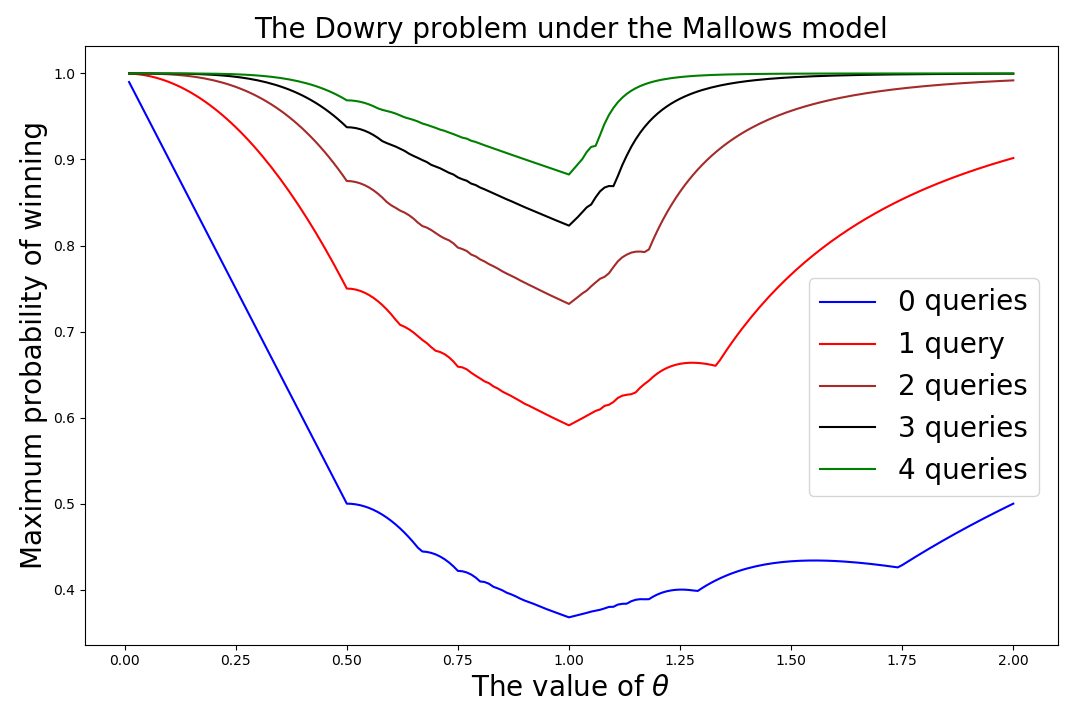
Figure 2: The maximum probability of success using our optimal strategy under the Mallows model.

6 Expected Number of Queries and Interviewed Candidates

The maximum probability of winning for the Dowry model with $s$ selections and the query-based model with $s-1$ queries are the same, as both models have a budget of $s$ selections and the goal is to choose the best candidate (note that this claim holds for all Mallows parameters, but that the Dowry problem has – until this work – only been studied for a uniform distribution of candidate orders for which $\theta=1$). However, the expected stopping times are very different. Under the query-based model, the process immediately terminates after obtaining a positive answer from the expert. On the other hand, the decision making entity continues to interview the remaining candidates after a selection is made (provided there is a selection left) under the Dowry setting, as it has no information about weather the current candidate is the best.

Furthermore, since a query to an expert is costly in practice, it is also of interest to examine the expected number of queries or interviews made during the process.

6.1 Expected Number of Queries

In this setting, we are interested in two expectations: Unconditional expectations: The expected number of selections made using the optimal strategy (described in Table 1); Conditional expectations: The expected number of selections made conditioned on the event that the best candidate is selected using the optimal strategy (described in Table 1).

Claim 43.

The conditional and unconditional expected number of selections for the query-based model is the same as for the Dowry model.

Proof.

Assume that under the query-based model we made a total $r$ selections, where $0\leq r\leq s$, using our optimal $(k_{1},\ldots,k_{s})$-strategy with $k_{i}=a_{s+1-i}(\theta),$ $1\leq i\leq s$. We show next that the Dowry model makes the same number of selections.

First, assume that $r=0$. Then the value $N$ is located at a position $j\leq k_{1}$, since otherwise there is at least one left-to-right maxima at a position in $[k_{1},N]$ and thus our optimal query strategy will result in at least one selection in both models.

Next, assume that $1\leq r\leq s-1$ and that the $r^{\text{th}}$ query is made at a position $j\geq k_{r}+1$. The value $N$ must be at a position $h$ such that $h\geq j$, since if $h<j$ there would have been no query at position $j$.

Under the above assumption, we proceed as follows. First, assume that $h=j$. In the Dowry model, the $1^{\text{st}}$, $\ldots$, $(r-1)^{\text{th}}$ selections/queries are the same as the expert keeps giving a negative answer. We then pick up the value $N$ at position $j$ (without knowing this fact in the Dowry model) and examine the list until the end; we do not make the $(r+1)^{\text{th}}$ selection since there is no left-to-right maxima after position $j$. Second, assume that $h>j$. Then we must have $h\leq k_{r+1}$ since otherwise the $(r+1)^{\text{th}}$ selection will be made. In the Dowry model, the $1^{\text{st}}$, $\ldots$, $(r-1)^{\text{th}}$, and $r^{\text{th}}$ selections are the same as those in the query-based model as the latter gives negative answers. We do not make another selection until position $k_{r+1}$ since the $(r+1)^{\text{th}}$ selection is not allowed until after position $k_{r+1}$, and we cannot perform the $(r+1)^{\text{th}}$ selection after position $k_{r+1}$ since there is no left-to-right maxima following position $h$.

The last case to consider is $r=s$. We used all $s-1$ queries to query an expert, received $s-1$ negative answers, and then made a final decision at position $j\geq k_{s}+1$. Under the Dowry model, we made the same $s-1$ selections, without knowing that they are not the best, then made the final selection at the same position $j$.

Similarly, we can show that if $r$, $1\leq r\leq s$, selections are made in the Dowry model then the same number of selections will be made using the query-based model. Similar arguments apply for the case when we condition on the event of identifying the best candidate.    $\Box$

Definition 44.

We call a permutation $\pi\in S_{N}$ exactly $r$-$(k_{1},\ldots,k_{s})$-winnable if the best value $N$ is selected as the $r^{\text{th}}$ selection when using the $(k_{1},\ldots,k_{s})$-strategy, where $1\leq r\leq s$. For simplicity, we abbreviate the name to $r$-winnable whenever the strategy is clear. Similarly to Definition 31, we define for $1\leq r\leq s$ that

$$W_{r}(N,k_{1},\ldots,k_{s})=\sum\limits_{r\text{-winnable }\pi\in S_{N}}\theta^{c(\pi)}.$$

Definition 45.

We call a permutation $\pi\in S_{N}$ exactly $r$-$(k_{1},\ldots,k_{s})$-pickable if it results in exactly $r$ selections using the $(k_{1},\ldots,k_{s})$-strategy, where $0\leq r\leq s$. We also abbreviate this reference to $r$-pickable whenever the strategy is clear. Similarly to Definition 32, we define for $0\leq r\leq s$ that

$$T_{r}(m,k_{1},\ldots,k_{s})=\sum\limits_{r\text{-pickable }\pi\in S_{N}}\theta^{c(\pi)}.$$

By Definition 31 and 44, the following result is straightforward.

Proposition 46.

One has $W(N,k_{1},\ldots,k_{s})=\sum\limits_{i=1}^{s}W_{i}(k_{1},\ldots,k_{s}).$

6.1.1 The Unconditional Expectations

By Definition 45, it is straightforward to see that the expected number of selections made using the $(k_{1},\ldots,k_{s})$-strategy equals

$$\sum\limits_{i=1}^{s}i\cdot\frac{T_{i}(N,k_{1},\ldots,k_{s})}{(P_{N})!}.$$

The following Lemma is a consequence of Definitions 32 and 45.

Lemma 47.

For $N\geq k_{s}+1$, we have $T_{0}(N,k_{1},\ldots,k_{s})=T_{0}(N,k_{1})$, and for $1\leq i\leq s$,

$$T_{i}(N,k_{1},\ldots,k_{s})=T_{\leq i}(N,k_{1},\ldots,k_{s})-T_{\leq i-1}(N,k_{1},\ldots,k_{s}).$$

Every permutation uses at most $s$ selections by the definition of the $(k_{1},\ldots,k_{s})$-strategy. By Lemma 36, when $\theta>1$ and $1\leq r\leq s$, we have

$$\lim\limits_{N\to\infty}\frac{T_{\leq r-1}(N,k_{1},\ldots,k_{s})}{(P_{N})!}=\lim\limits_{N\to\infty}\frac{T_{\leq r-1}(N,k_{1},\ldots,k_{r})}{(P_{N})!}=(1-\frac{1}{\theta^{k_{r}}})+$$

$$(1-\frac{1}{\theta})\cdot(1-\frac{1}{\theta^{k_{r-1}}})\cdot\sum\limits_{i=k_{r}}^{\infty}\frac{1}{\theta^{i}-1}+(1-\frac{1}{\theta})^{2}\cdot(1-\frac{1}{\theta^{k_{r-2}}})\cdot\sum\limits_{i_{1}=k_{r}}^{\infty}\frac{1}{\theta^{i_{1}}-1}\sum\limits_{i_{2}=k_{r-1}}^{i_{1}-1}\frac{1}{\theta^{i_{2}}-1}+\ldots+$$

$$(1-\frac{1}{\theta})^{r-1}\cdot(1-\frac{1}{\theta^{k_{1}}})\cdot\sum\limits_{i_{1}=k_{r}}^{\infty}\frac{1}{\theta^{i_{1}}-1}\sum\limits_{i_{2}=k_{r-1}}^{i_{1}-1}\frac{1}{\theta^{i_{2}}-1}\sum\cdots\sum\limits_{i_{r-1}=k_{2}}^{i_{r-2}-1}\frac{1}{\theta^{i_{r-1}}-1}.$$

When $0<\theta<1$ and $1\leq r\leq s$, we define $z_{r}=N-k_{r}$. Since $z_{1}=N-k_{1}\not\to\infty$,

$$\lim\limits_{N\to\infty}\frac{T_{\leq r-1}(N,k_{1},\ldots,k_{s})}{(P_{N})!}=\lim\limits_{N\to\infty}\frac{T_{\leq r-1}(N,k_{1},\ldots,k_{r})}{(P_{N})!}=\theta^{z_{r}}+$$

$$\theta^{z_{r-1}}\cdot(\frac{1}{\theta}-1)\cdot\lim\limits_{N\to\infty}\sum\limits_{i=k_{r}}^{N-1}1+\theta^{z_{r-2}}\cdot(\frac{1}{\theta}-1)^{2}\cdot\lim\limits_{N\to\infty}\sum\limits_{i_{1}=k_{r}}^{N-1}\sum\limits_{i_{2}=k_{r-1}}^{i_{1}-1}1+\ldots+$$

$$\theta^{z_{1}}\cdot(\frac{1}{\theta}-1)^{r-1}\cdot\lim\limits_{N\to\infty}\sum\limits_{i_{1}=k_{r}}^{N-1}\sum\limits_{i_{2}=k_{r-1}}^{i_{1}-1}\sum\ldots\sum\limits_{i_{r-1}=k_{2}}^{i_{r-2}-1}1.$$

6.1.2 The Unconditional Expectations

The expected number of queries made conditioned on successfully identifying the best candidate $N$ using the $(k_{1},\ldots,k_{s})$-strategy equals

$$\frac{\sum\limits_{i=1}^{s}i\cdot W_{i}(N,k_{1},\ldots,k_{s})/((P_{N})!)}{W(N,k_{1},\ldots,k_{s})/((P_{N})!)}=\frac{\sum\limits_{i=1}^{s}i\cdot W_{i}(N,k_{1},\ldots,k_{s})}{W(N,k_{1},\ldots,k_{s})}.$$

Assume that $N\geq k_{s}+1$ and observe that $\frac{W(N,k_{1},\ldots,k_{s})}{(P_{N})!}$ represents the probability of selecting the best candidate using the $(k_{1},\ldots,k_{s})$-strategy. Fix $k_{1},\ldots,k_{s}$. Since there can be at most $s$ selections when using the $(k_{1},\ldots,k_{s})$-strategy, $\frac{W(N,k_{1},\ldots,k_{s})}{(P_{N})!}$ represents the entity of interest when at most $s$ selections are made, $\frac{W(N,k_{1},\ldots,k_{s-1})}{(P_{N})!}$ represents the entity of interest when at most $s-1$ selections are made, $\ldots$, and $\frac{W(N,k_{1})}{(P_{N})!}$ represents the entity of interest when at most $1$ selection is made using the $(k_{1},\ldots,k_{s})$-strategy. This implies the following lemma.

Lemma 48.

For $N\geq k_{s}+1$, we have $W_{1}(N,k_{1},\ldots,k_{s})=W(N,k_{1})$, and for $2\leq i\leq s$,

$$W_{i}(N,k_{1},\ldots,k_{s})=W(N,k_{1},\ldots,k_{i})-W(N,k_{1},\ldots,k_{i-1}).$$

6.1.3 Numerical Results for $s=5$

Note that the opportunities to query an expert are always precious. Since we also want to maintain consistency with Section 5, we focus our attention on $s=5$. Both types of expectations based on the formulas from the previous subsections and for the optimal strategy described in Table 1 are listed in Table 2.

6.2 The Expected Number of Candidates Interviewed

The results for the query-based and the Dowry model differ in this setting. For the query-based model, we are informed when the best candidate is selected and thus stop interviewing. However, for the Dowry model, we do not have this information and will continue interviewing until the last candidate, except if we run out of selections.

The results below pertain to the case that we are performing interviews using a $(k_{1},\ldots,k_{s})$-strategy, where $k_{i}=a_{s+1-i}$ for each $1\leq i\leq s$. As before, we examine both the unconditional expectations and the conditional expectation given that best candidate is identified.

$\theta$	Unconditional	Conditional	$\theta$	Unconditional	Conditional
0.01	4.95	4.95	1.01	2.62667769	2.6972733
0.1	4.5	4.500045	1.02	2.62685978	2.68959942
0.2	4	4.00128041	1.03	2.59496416	2.66220979
0.3	3.5	3.50852572	1.04	2.79034804	2.80523622
0.4	3	3.03103783	1.05	2.64119948	2.68710199
0.5	2.5	2.58064516	1.06	2.49825217	2.57955508
0.6	2.7629312	2.81568154	1.07	3.29738824	3.17161865
0.7	2.64786481	2.71674096	1.08	3.20212123	3.09601664
0.8	2.6662117	2.73919532	1.09	3.12062719	3.02727948
0.9	2.63578947	2.71329095	1.10	3.04382379	2.96407481
0.91	2.61849239	2.69864672	1.2	2.54054933	2.52012037
0.92	2.63266523	2.70893875	1.3	2.26194433	2.25566216
0.93	2.63017179	2.70570293	1.4	2.07936215	2.07716359
0.94	2.63844464	2.71288008	1.5	1.94829005	1.94744469
0.95	2.62322511	2.7016097	1.6	1.84863362	1.84828375
0.96	2.62165305	2.69958325	1.7	1.76979138	1.76963762
0.97	2.6297567	2.70548721	1.8	1.70556686	1.70549578
0.98	2.62015186	2.69950777	1.9	1.65206303	1.65202872
0.99	2.61956681	2.69846554	2	1.60669004	1.60667284
			3	1.36430699	1.36430692
1	2.61986256	2.69822343	4	1.26329306	1.26329306
			5	1.20693541	1.20693541

Table 2: Unconditional and conditional expected number of selections used in the optimal strategies with $\theta>0$ and $s=5$.

6.2.1 The Query-based Model

Case 1: Unconditional expectations. Define

$$Y^{\prime}(m)=\sum\limits_{\begin{subarray}{c}\pi\in S_{N}\text{ s.t. we terminate at }m\\ \text{ using the $(k_{1},\ldots,k_{s})$-strategy}\end{subarray}}\theta^{c(\pi)}.$$

We are interested in

$$\sum\limits_{j=k_{1}+1}^{N}j\cdot\frac{Y^{\prime}(j)}{(P_{N})!}.$$

Let $k_{1}+1\leq m\leq N$. There are three cases to consider for the position $m$ at which we stop interviewing the candidates in $\pi$.

Case 1.1: $k_{i}+1\leq m\leq k_{i+1}$, where $1\leq i\leq s-1$. The position $m$ must contain the value $N$ and at most $i-1$ selections can be made before position $m$, since if the former constraint does not hold we will continue interviewing until the $s^{\text{th}}$ selection and if the latter constraint does not hold then we cannot select the best candidate at position $m$ and thus will not stop at position $m$.

Therefore,

$$Y^{\prime}(m)=\theta^{N-m}\cdot B(m-1,N-m)\cdot T_{\leq i-1}(k_{1},\ldots,k_{s})\cdot(P_{N-m})!=\frac{(P_{N-1})!}{(P_{m-1})!}\cdot\theta^{N-m}\cdot T_{\leq i-1}(m-1,k_{1},\ldots,k_{s}).$$

Case 1.2: $k_{s}+1\leq m\leq N-1$. Then interviews terminate at $m$ if either $m$ is a left-to-right maxima and all $s-1$ experts were queried before position $m$ (with a final selection left for position $m$); or position $m$ has value $N$ and at most $s-2$ experts were queried before position $m$. To see this, if we stop at position $m$ then position $m$ must be a left-to-right maxima and either no selection is left after the final selection at position $m$ (i.e., we cannot continue interviewing) or position $m$ has the value $N$ and there is at least one query left before interviewing position $m$ (thus we query the expert and get the answer that we found the best candidate and stop at position $m$).

In the former case, the first $m$ positions are arbitrary elements from $\{1,\ldots,N\}$; the $m^{\text{th}}$ position has the largest value among the first $m$ positions; and exactly $s-1$ selections were used for positions in $[1,m-1]$. Now, $T_{s-1}(m-1,k_{1},\ldots,k_{s})$ counts the inversions within the first $m$ positions, $(P_{N-m})!$ counts the inversions within positions $[m+1,N]$, while $B(m,N-m)$ counts the inversions between the two sets. Moreover, $\theta^{N-m}\cdot T_{\leq s-2}(m-1,k_{1},\ldots,k_{s})\cdot B(m-1,N-m)\cdot(P_{N-m})!$ accounts for the case when position $m$ has value $N$ and at most $s-2$ queries are made before position $m$.

Therefore,

$$Y^{\prime}(m)=B(m,N-m)\cdot T_{s-1}(m-1,k_{1},\ldots,k_{s})\cdot(P_{N-m})!+\theta^{N-m}\cdot T_{\leq s-2}(m-1,k_{1},\ldots,k_{s})\cdot B(m-1,N-m)\cdot(P_{N-m})!$$

$$=T_{s-1}(m-1,k_{1},\ldots,k_{s})\cdot\frac{(P_{N})!}{(P_{m})!}+\theta^{N-m}\cdot T_{\leq s-2}(m-1,k_{1},\ldots,k_{s})\cdot\frac{(P_{N-1})!}{(P_{m-1})!}.$$

Case 1.3: $m=N$. Since the interviewing process must stop at $N$ we have

$$Y^{\prime}(N)=(P_{N})!-\sum\limits_{j=k_{1}+1}^{N-1}Y^{\prime}(j).$$

Case 2: Conditional Expectations. Define

$$Y^{\prime\prime}(m)=\sum\limits_{\begin{subarray}{c}\pi\in S_{N}\text{ is $(k_{1},\ldots,k_{s})$-winnable and}\\ \text{the search terminates at }m\end{subarray}}\theta^{c(\pi)}.$$

We are interested in

$$\frac{\sum\limits_{j=k_{1}+1}^{N}j\cdot Y^{\prime\prime}(j)/(P_{N})!}{W(N,k_{1},\ldots,k_{s})/(P_{N})!}=\frac{\sum\limits_{j=k_{1}+1}^{N}j\cdot Y^{\prime\prime}(j)}{W(N,k_{1},\ldots,k_{s})}.$$

There are two cases to consider.

Case 2.1: $k_{i}+1\leq m\leq k_{i+1}$, where $1\leq i\leq s-1$. Then the value $N$ had to be at position $m$ and at most $i-1$ selections were made before position $m$, since position $m$ must contain the value $N$ in order for the process to terminate successfully, and since if $i$ selections were made before position $m$, one could not have choose the value $N$ at position $m$. Therefore, for this case

$$Y^{\prime\prime}(m)=\theta^{N-m}\cdot T_{\leq i-1}(m-1,k_{1},\ldots,k_{s})\cdot B(m-1,N-m)\cdot(P_{N-m})!=\frac{(P_{N-1})!}{(P_{m-1})!}\cdot\theta^{N-m}\cdot T_{\leq i-1}(m-1,k_{1},\ldots,k_{s}).$$

Case 2.2: $m\geq k_{s}+1$. Again the value $N$ had to be at position $m$ and at most $s-1$ selections had to be made before position $m$. Therefore, for this case

$$Y^{\prime\prime}(m)=\theta^{N-m}\cdot T_{\leq s-1}(m-1,k_{1},\ldots,k_{s})\cdot B(m-1,N-m)\cdot(P_{N-m})!=\frac{(P_{N-1})!}{(P_{m-1})!}\cdot\theta^{N-m}\cdot T_{\leq s-1}(m-1,k_{1},\ldots,k_{s}).$$

6.2.2 The Expectations for the Dowry Model

In the Dowry model, the aim is to use all $s$ selections, since we do not have the information whether each of our selection is the best or not. Hence, $m\geq k_{s}+1$.

Case 1: Unconditional Expectations. Define

$$Z^{\prime}(m)=\sum\limits_{\begin{subarray}{c}\pi\in S_{N}\text{ terminate at }m\\ \text{ using the $(k_{1},\ldots,k_{s})$-strategy}\end{subarray}}\theta^{c(\pi)}.$$

We are interested in

$$\sum\limits_{j=k_{s}+1}^{N}j\cdot\frac{Z^{\prime}(j)}{(P_{N})!}.$$

Case 1.1: $k_{s}+1\leq m\leq N-1$. We only care weather the $s^{\text{th}}$ selections is made at position $m$. Thus, for each subset $S$ of $m$ values of $\{1,\ldots,N\}$, since the largest value of $S$ must be placed at position $m$ and exactly $s-1$ selections had to be made before position $m$, we have that $T_{s-1}(m-1,k_{1},\ldots,k_{s})$ counts the number of inversions within the first $m$ positions for each fixed $S$; $B(m,N-m)$ counts the number of inversions between the two sets in the partition of $N$, $|\Pi_{1}|=m$ and $|\Pi_{2}|=N-m$, while $(P_{N-m})!$ counts the number of inversions within positions $[m+1,N]$. Therefore, in this case,

$$Z^{\prime}(m)=T_{s-1}(m-1,k_{1},\ldots,k_{s})\cdot B(m,N-m)\cdot(P_{N-m})!=T_{s-1}(m-1,k_{1},\ldots,k_{s})\cdot\frac{(P_{N})!}{(P_{m})!}.$$

Case 1.2: $m=N$. All cases not covered by Case 1.1 include terminating at the last position and thus in this case

$$Z^{\prime}(m)=(P_{N})!-\sum\limits_{j=k_{s}+1}^{N-1}Z^{\prime}(j).$$

Case 2: Conditional Expectations. Define

$$Z^{\prime\prime}(m)=\sum\limits_{\begin{subarray}{c}\pi\in S_{N}\text{ is $(k_{1},\ldots,k_{s})$-winnable}\\ \text{and terminates at }m\end{subarray}}\theta^{c(\pi)}.$$

The entity of interest is

$$\frac{\sum\limits_{j=k_{s}+1}^{N}j\cdot Z^{\prime\prime}(j)/(P_{N})!}{W(N,k_{1},\ldots,k_{s})/(P_{N})!}=\frac{\sum\limits_{j=k_{s}+1}^{N}j\cdot Z^{\prime\prime}(j)}{W(N,k_{1},\ldots,k_{s})}.$$

Case 2.1: Terminating at a position $k_{s}+1\leq j\leq N-1$ and identifying the optimal candidate. Then, the $s^{\text{th}}$ selection is made at position $m$ and position $m$ has value $N$. Therefore, in this case,

$$Z^{\prime\prime}(j)=\theta^{N-m}\cdot T_{s-1}(m-1,k_{1},\ldots,k_{s})\cdot B(m-1,N-m)\cdot(P_{N-m})!=\theta^{N-m}\cdot T_{s-1}(m-1,k_{1},\ldots,k_{s})\cdot\frac{(P_{N-1})!}{(P_{m-1})!}.$$

Case 2.2: Terminating at position $N$ and identifying the optimal candidate. It is possible that not all of the $s-1$ selections were used before and the best candidate was selected at position $N$; it is also possible that the best candidate was picked at some position in $[k_{s+1},N-1]$ but not all selections were used before the position $N$ and thus the search continued until after position $N$ (those two possibilities do not account for all possible cases). In this case,

$$\frac{Z^{\prime\prime}(N)}{(P_{N})!}=\frac{W(N,k_{1},\ldots,k_{s})}{(P_{N})!}-\sum\limits_{j=k_{s}+1}^{N-1}\frac{Z^{\prime\prime}(j)}{(P_{N})!}.$$

6.2.3 Numerical Results for $s=5$

We again focus our attention on $s=5$. Both types of expectations based on the formulas from the previous subsections and for the optimal strategy described in Table 1 are listed in Table 2.

Acknowledgment. The work was supported in part by the NSF grants NSF CCF 15-26875, CIF 1513373, through Rutgers University, and The Center for Science of Information at Purdue University, under contract number 239 SBC PURDUE 4101-38050. The work was done while X. Liu was with the University of Illinois, Urbana-Champaign.

7 Appendix

We make use of the following two results.

Theorem 49 (Jones [17], Theorem 6.5).

For $\theta<1$, the optimal asymptotic selection strategy for the secretary problem is to reject $N-j(\theta)\not\to\infty$ (not depending on $N$) candidates and then accept the next left-to-right maxima thereafter.

Theorem 50 (Jones [17], Corollary 6.6).

For $\theta>1$, the optimal asymptotic selection strategy for the secretary problem is to reject $j(\theta)\not\to\infty$ (not depending on $N$) candidates and then accept the next left-to-right maxima thereafter.

Proof of Theorem 41. The proof follows by induction.

First, note that $N-k_{1}\not\to\infty$ implies $N-k_{2},\ldots,N-k_{s}\not\to\infty$. The base case for one threshold hold by Theorem 49. We assume the argument works for $\leq s-1$ thresholds and prove the result for $s$-thresholds with $s\geq 2$.

By Lemma 38 and the fact $T_{\leq s-1}(k_{s},k_{1},\ldots,k_{s-1},k_{s})=(P_{k_{s}})!$, we have

$$\frac{W(N,k_{1},\ldots,k_{s})}{(P_{N})!}=\frac{1}{P_{N}}\cdot\Big{(}\frac{\theta^{N-k_{s}}\cdot P_{k_{s}}\cdot W(k_{s},k_{1},\ldots,k_{s-1})}{(P_{k_{s}})!}+\frac{T_{\leq s-1}(N-1,k_{1},\ldots,k_{s})}{(P_{N-1})!}+$$

$$\theta\cdot\frac{T_{\leq s-1}(N-2,k_{1},\ldots,k_{s})}{(P_{N-2})!}+\ldots+\theta^{N-k_{s}-2}\cdot\frac{T_{\leq s-1}(k_{s}+1,k_{1},\ldots,k_{s})}{(P_{k_{s}+1})!}+\theta^{N-k_{s}-1}\cdot 1\Big{)}.$$ (7)

Step 1: Suppose that $N-k_{s}\not\to\infty$ does not hold, i.e., that $N-k_{s}\to\infty$. Then, since the probability

$$\frac{W(k_{s},k_{1},\ldots,k_{s-1})}{(P_{k_{s}})!}\leq 1,\quad\text{ we have }$$

$$\frac{\theta^{N-k_{s}}\cdot P_{k_{s}}\cdot W(k_{s},k_{1},\ldots,k_{s-1})}{(P_{k_{s}})!}\to\frac{\theta^{N-k_{s}}}{1-\theta}\cdot\frac{W(k_{s},k_{1},\ldots,k_{s-1})}{(P_{k_{s}})!}\to 0.$$

Moreover, by Lemma 36, for $0\leq j\leq N-k_{s}-2$,

$$\theta^{j}\cdot\frac{T_{\leq s-1}(N-j-1,k_{1},\ldots,k_{s})}{(P_{N-j-1})!}=\frac{1}{P_{N-j-1}}\cdot\Big{(}\theta^{N-k_{s}-1}\cdot P_{k_{s}}+\theta^{N-k_{s-1}-2}\cdot P_{k_{s-1}}\cdot\sum\limits_{i=k_{s}}^{N-j-2}\frac{1}{P_{i}}+$$ (8)

$$\theta^{N-k_{s-2}-3}\cdot P_{k_{s-2}}\cdot\sum\limits_{i_{1}=k_{s}}^{N-j-2}\frac{1}{P_{i_{1}}}\sum\limits_{i_{2}=k_{s-1}}^{i_{1}-1}\frac{1}{P_{i_{2}}}+\ldots+\theta^{N-k_{1}-s}\cdot P_{k_{1}}\cdot\sum\limits_{i_{1}=k_{s}}^{N-j-2}\frac{1}{P_{i_{1}}}\cdot\sum\limits_{i_{2}=k_{s-1}}^{i_{1}-1}\frac{1}{P_{i_{2}}}\sum\cdots\sum\limits_{i_{s-1}=k_{2}}^{i_{s-2}-1}\frac{1}{P_{i_{s-1}}}\Big{)}.$$

For each term inside the bracket of (8), since $N-k_{i}\to\infty$, $\theta^{N-k_{i}}\to 0$ exponentially, and the sum part (without the multiplier) of each term approaches infinity as a polynomial function in $N-k_{i+1}\leq N-k_{i}$. The latter claim holds since $\frac{1}{P_{i}}=\frac{1-\theta}{1-\theta^{i}}\leq 1$ when $i\geq 1$ and the smallest value of the subscript equals $k_{2}\geq 1$.

Since $N-j-1\geq k_{s}+1$, we have

$$\theta^{j}\cdot\frac{T_{\leq s-1}(N-j-1,k_{1},\ldots,k_{s})}{(P_{N-j-1})!}\leq(\theta^{N-k_{s}-1}+\theta^{N-k_{s-1}-2}\cdot(N-k_{s-1})+\theta^{N-k_{s-2}-3}\cdot(N-k_{s-2})^{2}+\ldots$$

$$+\theta^{N-k_{1}-s}\cdot(N-k_{1})^{s-1})\leq s\cdot\max\limits_{q=1}^{s}\{\theta^{N-k_{q}-(s+1-q)}\cdot(N-k_{q})^{s-q}\}\to 0.$$

Above, the convergence rate $\to 0$ is exponential. Thus,

$$\frac{T_{\leq s-1}(N-1,k_{1},\ldots,k_{s})}{(P_{N-1})!}+\theta\cdot\frac{T_{\leq s-1}(N-2,k_{1},\ldots,k_{s})}{(P_{N-2})!}+\ldots+\theta^{N-k_{s}-2}\cdot\frac{T_{\leq s-1}(k_{s}+1,k_{1},\ldots,k_{s})}{(P_{k_{s}+1})!}+\theta^{N-k_{s}-1}$$

$$\leq(N-k_{s})\cdot s\cdot\max\limits_{q=1}^{s}\{\theta^{N-k_{q}-(s+1-q)}\cdot(N-k_{q})^{s-q}\}\leq s\cdot\max\limits_{q=1}^{s}\{\theta^{N-k_{q}-(s+1-q)}\cdot(N-k_{q})^{s+1-q}\}\to 0.$$

Step 2: Suppose that $N-k_{1}\not\to\infty$ does not hold, i.e., that $N-k_{1}\to\infty$.

From Step 1, we know that for an optimal strategy, $N-k_{s}\not\to\infty$ has to hold. We also know that $k_{s}-k_{1}\to\infty$. By the induction hypothesis,

$$\frac{W(k_{s},k_{1},\ldots,k_{s-1})}{(P_{k_{s}})!}\text{ is maximized when }k_{s}-k_{1}\not\to\infty(\text{ and is not maximized when }k_{s}-k_{1}\to\infty).$$ (9)

Moreover, for each $0\leq j\leq N-k_{s}-1$, by Lemma 36 and (8),

$$\theta^{j}\cdot\frac{T_{\leq s-1}(N-j-1,k_{1},\ldots,k_{s})}{(P_{N-j-1})!}\text{ is maximized when }N-k_{s},\ldots,N-k_{1}\not\to\infty.$$ (10)

To see why this is the case, say $N-k_{i}\to\infty$ and $N-k_{i+1}\not\to\infty$. Then the term involving $\theta^{N-k_{q}-(s+1-q)}$ approaches zero for $1\leq q\leq i$ (when $k_{1}=0$, the last term is zero by default).

Therefore, by (9) and (10),

$$\frac{W(N,k_{1},\ldots,k_{s})}{(P_{N})!}\text{ is maximized only when }N-k_{1}\not\to\infty,$$

which also implies $N-k_{1}\not\to\infty,\ldots,N-k_{s}\not\to\infty$.    $\Box$

Proof of Theorem 42: The proof proceeds by induction. For consistency, let $k_{0}=-1$ and $k_{s+1}=N$.

Note that $k_{s}\not\to\infty$ implies $k_{s-1},\ldots,k_{1}\not\to\infty$. By Theorem 50, the argument works for one threshold. Suppose now that the argument works for at most $s-1$ thresholds. We prove the claimed result for $s$ thresholds. To this end, we show that the choice $k_{i}\not\to\infty$ and $k_{i+1}\to\infty$ is always at least as good as the choice $k_{i-1}\not\to\infty$ and $k_{i}\to\infty$, where $1\leq i\leq s-1$.

Claim 51.

For the case $k_{i}\to\infty$ and $k_{i-1}\not\to\infty$, where $1\leq i\leq s$ we have

$$\frac{W(N,k_{1},\ldots,k_{s})}{(P_{N})!}\to\frac{W(k_{i},k_{1},\ldots,k_{i-1})}{(P_{k_{i}})!}.$$

Proof.

By Lemma 38 and $T_{\leq s-1}(k_{s},k_{1},\ldots,k_{s-1},k_{s})=(P_{k_{s}})!$,

$$\frac{W(N,k_{1},\ldots,k_{s})}{(P_{N})!}=\frac{1}{P_{N}}\cdot\Big{(}\frac{\theta^{N-k_{s}}\cdot P_{k_{s}}\cdot W(k_{s},k_{1},\ldots,k_{s-1})}{(P_{k_{s}})!}+\frac{T_{\leq s-1}(N-1,k_{1},\ldots,k_{s})}{(P_{N-1})!}+$$

$$\theta\cdot\frac{T_{\leq s-1}(N-2,k_{1},\ldots,k_{s})}{(P_{N-2})!}+\ldots+\theta^{N-k_{s}-2}\cdot\frac{T_{\leq s-1}(k_{s}+1,k_{1},\ldots,k_{s})}{(P_{k_{s}+1})!}+\theta^{N-k_{s}-1}\Big{)}.$$

$$=\quad\cdots=$$

$$\frac{1}{P_{N}}\cdot\Big{(}\frac{\theta^{N-k_{i}}\cdot P_{k_{i}}\cdot W(k_{i},k_{1},\ldots,k_{i-1})}{(P_{k_{i}})!}+$$

$$\frac{T_{\leq s-1}(N-1,k_{1},\ldots,k_{s})}{(P_{N-1})!}+\theta\cdot\frac{T_{\leq s-1}(N-2,k_{1},\ldots,k_{s})}{(P_{N-2})}+\ldots+\theta^{N-k_{s}-2}\cdot\frac{T_{\leq s-1}(k_{s}+1,k_{1},\ldots,k_{s})}{(P_{k_{s}+1})!}+\theta^{N-k_{s}-1}$$

$$+\quad\cdots\quad+$$

$$+\theta^{N-k_{i+1}}\cdot\frac{T_{\leq i}(k_{i+1}-1,k_{1},\ldots,k_{i})}{(P_{k_{i+1}-1})!}+\ldots+\theta^{N-k_{i}-2}\cdot\frac{T_{i}(k_{i}+1,k_{1},\ldots,k_{i})}{(P_{k_{i}+1})!}+\theta^{N-k_{i}-1}\Big{)}.$$ (11)

Since $T_{j}(m,k_{1},\ldots,k_{j+1})\leq(P_{m})!$,

$$\frac{T_{\leq s-1}(N-1,k_{1},\ldots,k_{s})}{(P_{N-1})!}+\theta\cdot\frac{T_{\leq s-1}(N-2,k_{1},\ldots,k_{s})}{(P_{N-2})!}+\ldots+\theta^{N-k_{s}-2}\cdot\frac{T_{\leq s-1}(k_{s}+1,k_{1},\ldots,k_{s})}{(P_{k_{s}+1})!}+\theta^{N-k_{s}-1}$$

$$+\quad\cdots\quad+$$

$$+\theta^{N-k_{i+1}}\cdot\frac{T_{\leq i}(k_{i+1}-1,k_{1},\ldots,k_{i})}{(P_{k_{i+1}-1})!}+\ldots+\theta^{N-k_{i}-2}\cdot\frac{T_{i}(k_{i}+1,k_{1},\ldots,k_{i})}{(P_{k_{i}+1})!}+\theta^{N-k_{i}-1}$$

$$\leq 1+\theta+\ldots+\theta^{N-k_{i}-1}=\frac{\theta^{N-k_{i}}-1}{\theta-1},$$

and thus $\leavevmode\nobreak\ \eqref{prob2}$ converges to

$$\frac{1}{1-1/(\theta^{N})}\cdot\Big{(}(1-1/\theta^{k_{i}})\cdot\frac{W(k_{i},k_{1},\ldots,k_{i-1})}{(P_{k_{i}})!}+(1/\theta^{k_{i}}-1/(\theta^{N}))\Big{)}\to\frac{W(k_{i},k_{1},\ldots,k_{i-1})}{(P_{k_{i}})!}\text{ as }k_{i}\to\infty.\hfill\qquad\Box$$

We compare the class of $(k_{1},\ldots,k_{s})$-strategies for which $k_{i-1}\not\to\infty$ (Case 1) and $k_{i}\to\infty$, with the class of $(k_{1},\ldots,k_{s})$-strategies for which $k_{i}\not\to\infty$ and $k_{i+1}\to\infty$ (Case 2).

Claim 52.

For every strategy $(k_{1}^{\prime},\ldots,k_{s}^{\prime})$ covered under Case 1 there is a strategy covered under Case 2 which performs better.

Proof.

Let $(k_{1}^{\prime},\ldots,k_{s}^{\prime})$ be a strategy with $k_{i-1}^{\prime}\not\to\infty$ and $k_{i}^{\prime}\to\infty$ (Case 1) and let $(k_{1}^{\prime\prime},\ldots,k_{s}^{\prime\prime})$ be a strategy such that $k_{j}^{\prime\prime}=k_{j}^{\prime}$ for $j\in\{1,\ldots,s\}-\{i\}$, $k_{i}^{\prime\prime}\not\to\infty$. Note that $k_{i}^{\prime\prime}\not\to\infty,k_{i+1}^{\prime\prime}\to\infty$ and thus the $(k_{1}^{\prime\prime},\ldots,k_{s}^{\prime\prime})$-strategy is also covered under Case 2.

By Claim 51, the probability of success for the $(k_{1}^{\prime},\ldots,k_{s}^{\prime})$-strategy is

$$\lim\limits_{k_{i}\to\infty}\frac{W(k_{i}^{\prime},k_{1}^{\prime},\ldots,k_{i-1}^{\prime})}{(P_{k_{i}^{\prime}})!}<\lim\limits_{k_{i+1}^{\prime\prime}\to\infty}\frac{W(k_{i+1}^{\prime\prime},k_{1}^{\prime\prime},\ldots,k_{i-1}^{\prime\prime},k_{i}^{\prime\prime})}{(P_{k_{i+1}^{\prime\prime}})!},$$

which is the winning probability for the $(k_{1}^{\prime\prime},\ldots,k_{s}^{\prime\prime})$-strategy since the latter case has one more selection than the former case and the value $k_{i}^{\prime\prime}$ can be placed anywhere as long as $k_{i}^{\prime\prime}\geq k_{i-1}^{\prime\prime}$ and $k_{i}^{\prime\prime}\not\to\infty$.    $\Box$

By Claim 52, the proof follows.    $\Box$

References

- [1] H. Ashtiani, S. Kushagra, S. Ben-David, “Clustering with same-cluster queries,” Advances in Neural Information Processing Systems (NIPS), pp. 3224–3232, 2016.
- [2] M. Babaioff, N. Immorlica, R. Kleinberg, “Matroids, secretary problems, and online mechanisms” ACM-SIAM Symposium on Discrete Algorithms (SODA), pp. 434–443, 2007.
- [3] I. Chien, C. Pan, and O. Milenkovic, “Query k-means clustering and the double dixie cup problem,” Advances in Neural Information Processing Systems (NeurIPS), 31, pp. 6649-6658, 2018.
- [4] M. Crews, B. Jones, K. Myers, L. Taalman, M. Urbanski and B. Wilson, “Opportunity Costs in the Game of Best Choice, ” The Electronic Journal of Combinatorics, vol. 26, no. 1, #P1.45, 2019.
- [5] E.B. Dynkin, “The optimal choice of the stopping moment for a Markov process,” Dokl. Akad. Nauk. SSSR, vol. 150, pp. 238–240, 1963.
- [6] T. Ferguson, “Who solved the secretary problem?,” Statistical science, Vol. 4, no. 3, pp. 282–289,1989.
- [7] A. Fowlkes and B. Jones, Positional strategies in games of best choice, Involve, vol. 12, no. 4, 647–658, 2019. MR 3941603
- [8] P. R. Freeman, “The secretary problem and its extensions - A review,” Internat. Statist. Rev. vol.51, pp. 189–206, 1983.
- [9] R. Freij, J. Wastlund, “Partially ordered secretaries,” Electron Commun Probab, vol. 15, pp. 504–507, 2010.
- [10] W. Huleihel, A. Mazumdar, M. Medard, and S. Pal, “Same-cluster querying for overlapping clusters,” Advances in Neural Information Processing Systems (NeurIPS), 30, pp. 10485-10495, 2019.
- [11] M. Gardner, “Mathematical games”, Scientific American, vol. 202, no. 2, pp. 152, 1960a.
- [12] M. Gardner, “Mathematical games”, Scientific American, vol. 202, no. 3, pp. 178–179, 1960b.
- [13] B. Garrod and R. Morris, “The secretary problem on an unknown poset,” Random Structures & Algorithms, vol. 43, pp. 429–451, 2012.
- [14] N. Georgiou, M. Kuchta, M. Morayne, J. Niemiec, “On a universal best choice algorithm for partially ordered sets”, Random Structures & Algorithms, vol. 32, pp. 263–273, 2008.
- [15] J. Gilbert and F. Mosteller, “Recognizing the maximum of a sequence,” J. Amer. Statist. Assoc., vol. 61, pp. 35–73, 1966.
- [16] B. Jones, “Avoiding patterns and making the best choice,” Discrete Mathematics, vol. 342, no. 6, pp.1529-1545, 2019.
- [17] B. Jones, “Weighted games of best choice,” SIAM Journal on Discrete Mathematics, vol. 34, no. 1, pp. 399–414, 2020.
- [18] U. Krengel and L. Sucheston, “On semiamarts, amarts, and processes with finite value”, Probability on Banach spaces, Adv. Probab. Related Topics, vol. 4, pp. 197–266. Dekker, New York, 1978.
- [19] D.V. Lindley, “Dynamic programming and decision theory,” Appl. Statist., vol.10, pp. 39–52, 1961.
- [20] X. Liu and O. Milenkovic, “The Postdoc Problem under the Mallows Model,” 2021 IEEE International Symposium on Information Theory (ISIT), pp. 3214–3219.
- [21] X. Liu and O. Milenkovic, “Finding the second-best candidate under the Mallows model”, Theoretical Computer Science, vol. 929, pp.39–68.
- [22] C. L. Mallows, “Non-null ranking models,” Biometrika, vol. 44, no. 1/2, pp. 114–130, 1957.
- [23] A. Mazumdar and B. Saha, “Clustering with noisy queries,” Advances in Neural Information Processing Systems (NIPS), pp. 5788-5799, 2017.
- [24] J. Preater, “The best-choice problem for partially ordered objects”, Oper Res Lett, vol. 25, pp. 187–190, 1999.
- [25] J. S. Rose, “A problem of optimal choice and assignment,” Operations Research, vol. 30, pp. 172–181, 1982.
- [26] J.A. Soto, “Matroid secretary problem in the random assignment model”, ACM-SIAM Symposium on Discrete Algorithms (SODA), pp. 1275–1284, 2011.
- [27] R. J. Vanderbei, “The postdoc variant of the secretary problem,” Technical report, Princeton University, Tech. Rep., 2012.