Observing and modelling the young solar analogue EK Draconis: starspot distribution, elemental abundances, and evolutionary status

Abstract

Observations and modelling of stars with near-solar masses in their early phases of evolution are critical for a better understanding of how dynamos of solar-type stars evolve. We examine the chemical composition and the spot distribution of the pre-main-sequence solar analogue EK Dra. Using spectra from the HERMES Spectrograph (La Palma), we obtain the abundances of 23 elements with respect to the solar ones, which lead to a $[{\rm Fe/H}]=0.03$, with significant overabundance of Li and Ba. The s-process elements Sr, Y, and Ce are marginally overabundant, while Co, Ni, Cu, Zn are marginally deficient compared to solar abundances. The overabundance of Ba is most likely due to the assumption of depth-independent microturbulent velocity. Li abundance is consistent with the age and the other abundances may indicate distinct initial conditions of the pre-stellar nebula. We estimate a mass of 1.04 $M_{\odot}$ and an age of $27^{+11}_{-8}$ Myr using various spectroscopic and photometric indicators. We study the surface distribution of dark spots, using 17 spectra collected during 15 nights using the CAFE Spectrograph (Calar Alto). We also conduct flux emergence and transport (FEAT) simulations for EK Dra’s parameters and produce 15-day-averaged synoptic maps of the likely starspot distributions. Using Doppler imaging, we reconstruct the surface brightness distributions for the observed spectra and FEAT simulations, which show overall agreement for polar and mid-latitude spots, while in the simulations there is a lack of low-latitude spots compared to the observed image. We find indications that cross-equatorial extensions of mid-latitude spots can be artefacts of the less visible southern-hemisphere activity.

forestgreenrgb0.00, 0.30, 0.00 purplergb0.50, 0.0, 0.50

1 Introduction

Monitoring young solar analogues is of key importance in determining patterns of magnetic activity on the Sun during its early stages of evolution (e.g. Kriskovics et al., 2019). Such observations are essential for testing theoretical models of the physical processes underlying stellar magnetic activity, namely, the generation, emergence, and surface transport of magnetic flux in solar-type stars. A fundamental problem awaiting explanation is the surface distribution of spots on such young and active stars, which is very different from solar patterns. In addition, investigating magnetic activity in young solar analogues is of great importance in understanding the angular momentum evolution (Cang et al., 2020) and the stellar dynamo, as they strongly affect each other throughout stellar evolution (Güdel, 2007; Brun & Browning, 2017). Probing stellar magnetic activity also holds special interest, since magnetic activity has important effects on the structure and evolution of planetary atmospheres (Johnstone, 2017), as well as detectability of exoplanets (Aigrain et al., 2016).

Doppler Imaging (hereafter DI) is a widely used technique in reconstructing distributions of relative brightness (or temperature) on the visible parts of rapidly rotating cool stars (see, Strassmeier, 2009). For a realistic Doppler image, three critical prerequisites are (a) a sufficiently large rotation rate and a good coverage of rotational phases, (b) a precise determination of fundamental stellar parameters, (c) high-resolution spectra with sufficiently high signal-to-noise ratios.

Using high-resolution spectra, detailed profiles of the chemical composition can also be obtained. This gives insight for studies of solar-like magnetic activity throughout stellar evolution, such as the Li abundance, which is often used as an indicator of the stellar age (see, e.g., Carlos et al., 2016). Elemental abundances are also important in revealing the initial chemical compositions of stellar birthplaces, and to evaluate the effects of metallicity on magnetic activity (Karoff et al., 2018).

In this study, we infer the starspot distribution using time-series of high-resolution spectra. We also carry out an extensive chemical abundance analysis for a large number of elements aiming to derive the abundance pattern for the atmosphere of EK Dra, and compare this with the solar elemental abundances. To interpret the observed Doppler images, we synthesise artificial ones, by applying the flux emergence and transport model developed by Işık et al. (2018), considering the age of EK Draconis.

1.1 EK Dra

EK Dra (G1.5V) can be considered as a laboratory to characterise the magnetic activity of a solar-type star at its early stages of evolution. Various ages between 30 and 125 Myr are proposed for EK Dra (see, e.g. Soderblom & Clements, 1987; Stauffer et al., 1998; Wichmann et al., 2003; König et al., 2005; Järvinen et al., 2007). It is the primary component of a widely separated binary system. The mass of the secondary component is about $0.5~{}M_{\odot}$ (König et al., 2005). EK Dra rotates at a rate of about 10 times that of the Sun (recently given by Järvinen et al. (2018) as $P_{\rm rot}\sim 2.606$ km/s).

The first Doppler Image (hereafter DI) of this young solar analogue was performed by Strassmeier & Rice (1998), using high-resolution CFHT spectra obtained in 1995. They found several cool spots distributed throughout low- to mid-latitudes, while the dominant spot was located at around 70-80^∘ latitudes. They estimated spots with temperature deficits in the range between 400-1200 K. Using photometric data gathered between 1994-1998, they pointed out that a high-latitude feature can be responsible for the continuous decline of the mean brightness. Fröhlich et al. (2002) performed long-term photometry covering 35 years, using Sky-Patrol plates obtained at Sonneberg Observatory and found a secular dimming of 0.0057 $\pm{0.0008}$ mag/yr within the observation time-range considered. Järvinen et al. (2005) analyzed V-band photometric data of EK Dra covering 21 years using light curve inversions and found that the system shows long-lived, non-axisymmetric spot distribution with active longitudes on opposite hemispheres. König et al. (2005) calculated the masses of the primary and secondary components as 0.9$M_{\rm\odot}$ and 0.5$M_{\rm\odot}$, respectively, and found that the orbit of the binary system is highly eccentric with $e=0.82$, using a combination of speckle observations and radial velocity measurements. They also obtained the effective temperature, $T_{\rm eff}$, as 5700 K and the surface gravity, $\log g$, as 4.37, using high-resolution spectra. In another detailed study of EK Dra, Järvinen et al. (2007) found both high- and low-latitude spots 500 K cooler than the quiet photosphere, using the inversions of atomic line profiles and mentioned both equatorward and poleward migration of spots around active longitudes. Furthermore, they pointed out that the equivalent widths of CaII-IRT emission cores increased during the light-curve minimum, indicating a positive correlation between photospheric and chromospheric activity. From a detailed model-atmosphere analysis of high-resolution spectra of EK Dra, they obtained $T_{\rm eff}$=5750 K, logg=4.5, and the microturbulent velocity, $\xi$, as 1.6 km/s. They estimated an age between 30-50 Myr.

Järvinen et al. (2009) studied EK Dra, based on additional spectra obtained in 2007. They also inferred high-latitude spot concentrations. Rosén et al. (2016) published two brightness maps, along with vector magnetic maps, using spectra obtained in 2007 and 2012. They found spots covering all longitudes and a wide latitudinal range, excluding high-latitude regions above $\sim 60^{\circ}$.

Waite et al. (2017) reconstructed brightness and magnetic maps using spectropolarimetric observations covering six years of data obtained at the CFHT and TBL observatories between 2006 and 2012. Their surface reconstructions between 2006 and 2007 show large spots located at intermediate latitudes, while the maps based on 2008 data show a dominant polar spot region. The maps also showed significant spot evolution over three-month periods, which the authors interpreted as rapid reorganisation of the global magnetic field. Using Stokes V data, they also obtained an average equatorial rotational velocity ($\Omega_{\rm eq}\sim 2.50\pm 0.08~{}{\rm rad~{}d}^{-1}$) as well as a surface differential rotation rate with an average rotational shear of $\Delta\Omega\sim 0.27^{+0.24}_{-0.26}~{}{\rm rad~{}d}^{-1}$.

The most recent Doppler imaging study of EK Dra was carried out by Järvinen et al. (2018) (hereafter J18), using a time series of very high resolution intensity spectra obtained at the Large Binocular Telescope equipped with the Potsdam Echelle Polarimetric and Spectroscopic Instrument (PEPSI). Using 10 spectra obtained between April 3 - 11 2015, they reconstructed a temperature map including 4 distinctive cool spots located at mid- to low latitudes, with temperature differences ranging from 280 K to 990 K with respect to the photosphere.

There are only two studies conducting a detailed analysis of the abundances of several chemical elements for EK Dra. However, both of these studies are based on automated spectral synthesis modelling methods. Valenti & Fischer (2005) derived the abundances of Na, Si, Ti, Fe, and Ni elements with respect to the solar abundances. [Na/H], [Si/H], and [Ni/H] are derived as -0.04 dex indicating solar-like values. However, they find [Ti/H]=$0.15\pm 0.05$ and [Fe/H]=$0.16\pm 0.03$, which are marginally larger than the solar abundances. Brewer et al. (2016) also derived the abundances of 15 elements. The abundances of C, Si, V, Cr, Mn, Fe, and Y are derived to be very close to the solar ones, i.e., within $\pm 0.06$ dex. However, they derived slightly larger abundances (0.11-0.22 dex) for N, O, and Ca, and slightly smaller abundances (between -0.13 and -0.19) for Na, Mg, Al, and Ni, with respect to the solar abundances. In addition to these studies, König et al. (2005), Järvinen et al. (2007), and Järvinen et al. (2018) reported ${\rm[Fe/H]}=-0.16\pm 0.02$, $0.00\pm 0.05$, and $-0.20\pm 0.02$, respectively, from the spectrum synthesis. König et al. (2005) and Järvinen et al. (2007) also derived the lithium abundance log $(N_{Li})$ for the star as $3.02\pm 0.02$ and $3.30\pm 0.05$, respectively.

2 Observations and Data Reduction

The high resolution time-series spectra of EK Dra were obtained between 17 and 31 July, 2015 with the CAFE spectrograph (Aceituno et al., 2013) attached to the 2.2 m telescope at the Calar Alto Observatory (Almeria, Spain) and with the HERMES spectrograph (Raskin et al., 2011) attached to the 1.2 m Mercator telescope at the Roque de los Muchachos Observatory (La Palma, Spain) between 15 December 2015 and 17 May 2016. During the Calar Alto run, we obtained 17 spectra covering a wavelength range between 4050Å - 9095 Å and an average resolution of R=62000, while we obtained 12 spectra of EK Dra with an average resolution of R=85000 and a wavelength coverage between 3780 - 9007 Å. The log of observations including Signal-to-Noise Ratio (SNR) values is given in Table 1. We also observed slowly-rotating and non-active template stars HD 143761 (G0 V), HD146233 (G2 V), HD 4628 (K2.5 V) and HD 22049 (K2 V) during the observing runs. The ephemeris used for the phase calculation of the spectral data obtained in this study is taken from Järvinen et al. (2018) and given in equation 1 below:

$${\rm HJD}=2445781.8590+2^{\rm d}.606\times E.$$ (1)

As seen from Table 1, we have good phase coverage of EK Dra; 17 spectra covering 15 days were obtained from CAFE in July 2015. On the other hand, for the HERMES run, the spectral data covers 6 months distributed among December 2015, March 2016 and May 2016. Therefore, we used the CAFE data only for Doppler Imaging, while the HERMES data is used only for abundance analysis, since such intermittent coverage over such a length of time is not ideal for DI. In addition, the CAFE data used for the DI procedure almost uniformly samples the rotation period of the star, in fact it has the densest spectral coverage compared to previous DI studies. The reduction procedures such as bias and flat correction, removal of cosmic rays, wavelength calibration and heliocentric velocity correction for the Calar Alto data were performed with the help of the IRAF (Image Reduction and Analysis Facility) standard packages. For the reduction process of HERMES data, we used the automatic pipeline of the spectrograph (Raskin et al., 2011).

We applied the signal enhancing Least Squares Deconvolution (LSD) technique (Donati et al., 1997) to obtain high SNR profiles of the spectral data. The LSD routine is based on a cross-correlation technique that combines photospheric lines in the observed spectrum into a single profile in the velocity space to enhance the SNR value. The line list required by the LSD technique was derived from the Vienna Atomic Line Database (VALD) (Kupka et al., 1999), considering the effective temperature ($T_{\rm eff}$) and the surface gravity ($\log g$) of EK Dra. During the preparation of the line list, wavelength regions covering chromospheric lines as well as the strong telluric lines were extracted to prevent any artefacts in the LSD profiles. The LSD profiles of the template stars were also obtained, which are used for the generation of lookup tables to model the local intensity profile during DI process. The resolving power of R=62000 allows us to generate the velocity profiles with 2.5 km/s intervals.

Table 1: Phase-ordered spectroscopic observation log of EK Dra.

Date	Exp. Time (sec.)	PhaseMid	SNR
Calar Alto Observing run
18.07.2015	1800	0.069	90
19.07.2015	1800	0.135	77
21.07.2015	2200	0.220	115
22.07.2015	2200	0.267	88
29.07.2015	1800	0.284	58
30.07.2015	1800	0.339	69
19.07.2015	1800	0.495	90
27.07.2015	1800	0.536	83
22.07.2015	2300	0.597	115
22.07.2015	2300	0.644	80
30.07.2015	1800	0.671	90
17.07.2015	1800	0.679	81
31.07.2015	1800	0.720	70
20.07.2015	2000	0.834	103
21.07.2015	2200	0.885	93
28.07.2015	1800	0.909	93
29.07.2015	1800	0.961	55
La Palma Observing run
25.03.2016	1200	0.107	131
17.12.2015	1200	0.164	134
28.03.2016	1200	0.259	154
16.05.2016	1200	0.359	100
15.12.2015	1200	0.401	96
26.03.2016	1200	0.491	109
29.03.2016	1200	0.646	155
17.05.2016	1200	0.735	147
27.03.2016	1000	0.870	145
19.12.2015	1200	0.939	111
15.05.2016	1800	0.963	96
15.05.2016	1200	0.985	107

3 Fundamental Parameters

We have estimated the effective temperature ($T_{\rm eff}$), surface gravity ($\log g$), rotational velocity ($v{\rm sin}i$), microturbulence ($\xi$), distance, mass ($M$), radius ($R$), and age ($\tau$) of EK Dra using various photometric and spectroscopic methods. The results and adopted values are summarised in Table 2. The uncertainties of the adopted atmospheric parameters were estimated from the standard deviations of the individual measurements.

Table 2: Fundamental Parameters of EK Dra.

Parameter	Valuea	Method and notes
$T_{{\rm eff}}\ [K]$	$5672$	Strömgren photometry
	$5811\pm 65$	Geneva photometry
	$5799\pm 100$	Johnson photometry + F96
	$5926\pm 100$	Johnson photometry + B98
	$5776\pm 100$	Johnson photometry + SF00
	$5770\pm 120$	SDSS $g$ and $r$ filters + B12
	$5664\pm 120$	Gaia photometry + B12
	$5770\pm 50$	Excitation eq. of Fe I
	$5770\pm 80$	Adopted
Log $g$ [cgs]	$4.41$	Strömgren photometry
	$4.28\pm 0.26$	Geneva photometry
	$4.54\pm 0.15$	SDSS $g$ and $r$ filters + B12
	$4.46\pm 0.12$	Gaia photometry + B12
	$4.40\pm 0.10$	Ion. eq. of Ti I/II and Cr I/II
	$4.4\pm 0.1$	Adopted
$\xi_{{\rm mic}}$ [km s-1]	$1.7\pm 0.1$	by minimizing $\sigma_{{\rm[Fe/H]}}$
Dist. [pc]	$34.45\pm 0.03$	Gaia parallax
$M$ [$M_{\rm\odot}$]	$1.04\pm 0.04$	$T_{\rm eff}-{\rm log}g$ diagram + B12
$R$ [$R_{\rm\odot}$]	$1.07\pm 0.10$	$T_{\rm eff}-{\rm log}g$ diagram + B12
Log $\tau\rm{{}^{b}}$	$\lesssim 7.7$	From Li abundance
	$7.43\pm 0.15$	$T_{\rm eff}-{\rm log}g$ diagram + B12
		(Adopted)
vsin$i$ [km s-1]	$17.0\pm 0.5$	From Fe I lines
	$16.6\pm 0.2$	From DI (Adopted)
vrad [km s-1]	$-20.26\pm 0.01$	From DI
$i$ [∘]	$63$	From J18

^a Systematic uncertainties caused by isochrones (B12) were assumed as $\pm 0.1$ dex for log $g$ and $\pm 100$ K for $T_{{\rm eff}}$.
^b $\tau$: age in years.

The magnitudes of EK Dra in Johnson ($BV$), Geneva ($UB_{1}B_{2}V_{1}G$), and Strömgren ($uvby$) systems were collected from Hipparcos/Tycho catalogue (ESA, 1997), Rufener (1988), Olsen (1983), and Hauck & Mermilliod (1998). $T_{\rm eff}$ and log $g$ of the star were initially derived using the photometric calibrations of Flower (1996, F96), Bessell et al. (1998, B98), Sekiguchi & Fukugita (2000, SF00), Kunzli et al. (1997, K97), and Napiwotzki (1997, N97). The distance of the star was calculated to be $35\pm 0.4$ pc from its Gaia DR2 parallax Gaia Collaboration et al. (2016, 2018). The colour excess of the star was derived to be $E(b-y)=0.002$ from Strömgren photometry. At the distance and galactic position of EK Dra, the 3D dust map of Green et al. (2015) also gave a null (i.e., $E(B-V)=0.00$) colour excess. The colour excess of the star was therefore neglected for all photometric systems.

Besides the photometric calibrations in Strömgren and Geneva systems, we also estimate the atmospheric parameters of EK Dra using colour-magnitude diagrams with theoretical isochrones for Gaia DR2 (G, $G_{\rm BP}$ and $G_{\rm RP}$) and SDSS DR14 ($gr$) magnitudes. The isochrones were taken from PARSEC (Bressan et al., 2012, B12). We chose the isochrones computed for Weiler’s (2018) Gaia filter transmissions proposed for bright stars. The mean of these photometrically estimated $T_{\rm eff}$ and $\log g$ values were refined further through spectroscopic methods (see Sec. 4 for the details) and the final atmospheric parameters were derived as $T_{{\rm eff}}=5770\pm 80$ K and log $g=4.4\pm 0.1$. We then plotted the star on the $T_{\rm eff}-{\rm log}g$ diagram (Fig. 1) and estimated the mass, radius, and the age of the star. A mass of $1.04\pm 0.04$ M$\odot$ and an age of log $\tau=7.43\pm 0.15$ (i.e., $27^{+11}_{-8}$ Myr) were consequently estimated, putting EK Dra on the pre-main sequence phase of its evolution, most likely in the post-T Tauri stage.

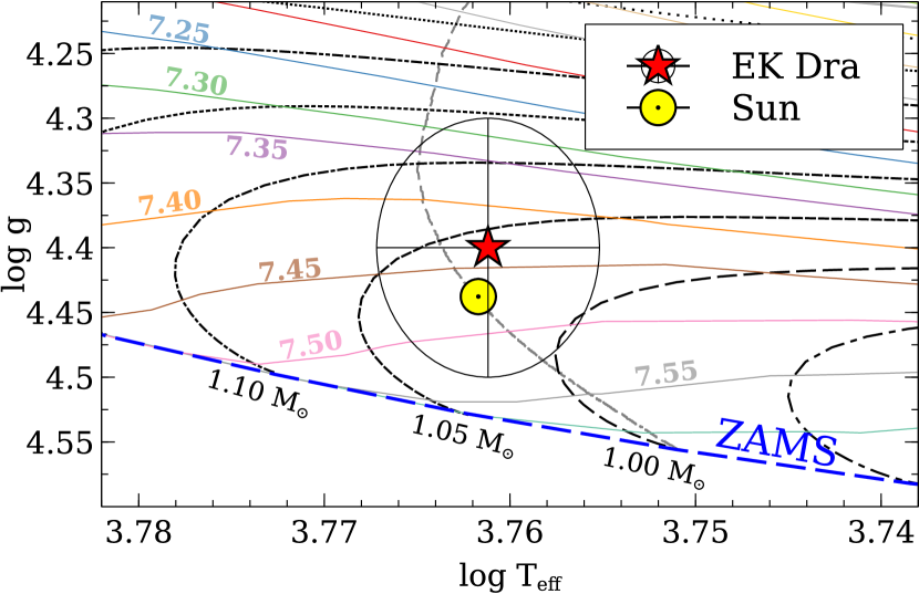
Figure 1: EK Dra on a $T_{\rm eff}-{\rm log}g$ diagram with PARSEC isochrones and pre-main sequence (PMS) evolutionary tracks. The masses are shown below each evolutionary track. The logarithm of the ages (log $\tau$, $\tau$ in years) are also shown above each isochrone with corresponding colour codes (we note that these ages are only valid for PMS stars). The theoretical position of the Sun and its main-sequence evolutionary track (dashed gray line) are displayed only for a comparison purpose. All tracks and isochrones are for the initial metallicity $z=0.01774$.

4 Chemical Abundance Analysis

The model atmospheres were computed with ATLAS12 (Kurucz, 1993; Sbordone et al., 2004) assuming Local Thermodynamic Equilibrium (LTE) and plane-parallel geometry. For the spectrum synthesis, the atomic data was retrieved from VALD (Piskunov et al., 1995; Ryabchikova et al., 1997; Kupka et al., 1999, 2000) and the NIST database (Kramida et al., 2015). The detailed list of the atomic lines can be found in Kılıçoğlu et al. (2016). The oscillator strengths of ⁷Li lines were adopted from Reddy et al. (2002). The mixing length parameter were calculated to be $\alpha=1.53$ from the calibration of Ludwig et al. (1999).

In order to avoid photospheric activity as much as possible, we selected spectra obtained by the HERMES spectrograph when the star is in a less active phase, i.e., the spectra have weak emission features in the Ca II H&K lines. Three out of 12 observed HERMES spectra, obtained consecutively on March 29th, 2016, fitted this condition. We merged these three spectra to increase the S/N and used the merged spectrum for chemical abundance analysis. We carefully selected 434 unblended (or barely blended) lines of Li, C, Na, Mg, Al, Si, S, Ca, Sc, Ti, V, Cr, Mn, Fe, Co, Ni, Cu, Zn, Sr, Y, Ba, Ce, and Nd in the spectrum. We then fitted these observed spectra line-by-line with synthetic profiles produced by SYNSPEC49 and its SYNPLOT interface. The code was modified to minimise the $\chi^{2}$ between the model and the observed points, using the Levenberg-Marquardt algorithm (Markwardt, 2009). The rotational velocity was derived to be $v$sin$i$ = $17.0\pm 0.5$ km s^-1 by adjusting the synthetic spectra to the unblended iron lines.

To derive the microturbulent velocity of EK Dra, we obtained the iron abundance [Fe/H] using 190 unblended Fe I lines for a set of microturbulent velocities ranging from 0.0 to 4.0 km s^-1. Figure 2 shows the standard deviation of the derived ${\rm[Fe/H]}$ as a function of the microturbulent velocity. The adopted microturbulent velocity is the value which minimises the standard deviation, i.e., $\xi=1.72\pm 0.10$ km s^-1. The abundances of the other elements were determined after this step using the obtained $\xi$ value.

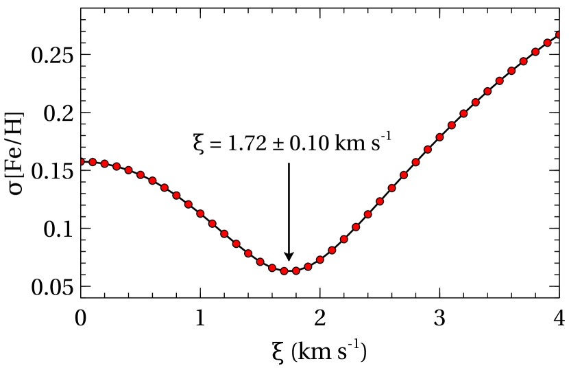
Figure 2: Standard deviation of the derived iron abundance vs. the microturbulent velocity for EK Dra.

The atmospheric parameters of EK Dra were refined by testing the excitation equilibrium of Fe I and the ionisation equilibrium of Ti I/II and Cr I/II. The scatter plot of excitation potential vs. Fe abundances (from Fe I lines) gave the minimum regression slope at $T_{\rm eff}=5770$ K (Fig. 3). For log $g$=4.4, we derived the same Cr abundance from both Cr I and Cr II lines, and the same Ti abundances from both Ti I and Ti II lines (within $\pm 0.02$ dex). We could not use Fe lines for ionisation equilibrium because there were an insufficient number of Fe II lines in the spectra for the analysis. These atmospheric parameters therefore provided reasonable ionisation and excitation equilibria for the star.

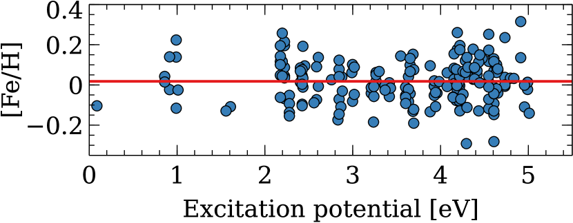
Figure 3: [Fe/H] versus excitation energies of the Fe I lines for $T_{\rm eff}=5770$ K. Red regression line with a slope of 0.0 confirms the excitation equilibrium.

We performed a detailed uncertainty analysis for the chemical abundances. Within the uncertainty limits, we altered $T_{\rm eff}$, $\log g$, and $v_{\rm mic}$ parameters of the synthetic spectrum and re-derived the abundances for each variation. We also derived standard errors ($\sigma^{2}_{\rm sterr}$) of the abundances derived from individual lines for each element. Therefore, the uncertainties given in Table 3 are calculated using the assumption below:

$$\sigma_{\rm tot}=\sqrt{\sigma^{2}_{T_{\rm eff}}+\sigma^{2}_{{\rm log}g}+\sigma^{2}_{\rm\xi}+\sigma^{2}_{\rm sterr}}$$

The final abundances of 23 elements are given in Table 3 and the deviations from the solar abundances (taken from Grevesse & Sauval, 1998) are illustrated in Fig. 4. We have detected significant overabundances of Li and Ba (Fig. 5). The 3D non-LTE (NLTE) correction for Li abundance $\Delta A({\rm Li})=0.07$ has been adopted from Harutyunyan et al. (2018). The lithium abundance $A_{\rm NLTE}({\rm Li})$$=3.35$ we measure is quite large and comparable with that of T Tauri stars. This shows that there is no remarkable Li depletion for EK Dra. Martin et al. (1992) have reported that most of the lithium depletion occurs in the last stage of pre-main-sequence evolution, i.e., about 50 Myr for $1.0\,M_{\odot}\lesssim M\lesssim 1.1\,M_{\odot}$. Therefore, the photospheric lithium abundance of EK Dra indicates that the star is most likely younger than $\sim{}50$ Myr, and this age limit agrees well with the age we found from the $T_{\rm eff}-{\rm log}g$ diagram ($27^{+11}_{-8}$ Myr). The cause of the Ba overabundances seen in very young chromospherically active stars has recently been investigated by Reddy & Lambert (2017). They concluded the Ba abundances could be overestimated due to the depth-independent microturbulence approximation: the line forming layer of Ba II is much higher than that of Fe, and consequently, larger microturbulent velocities are needed to model the Ba II lines. In their Fig 10., stars with larger chromospheric activity index log $R^{\prime}_{\rm HK}$ tend to exhibit larger Ba abundances (from Ba II lines). The activity index of EK Dra has been reported to be log $R^{\prime}_{\rm HK}=-4.19\pm 0.04$ by Rosén et al. (2016) and log $R^{\prime}_{\rm HK}=-4.08\pm 0.05$ by Boro Saikia et al. (2018). Using a rough extrapolation from the Fig 10. of Reddy & Lambert (2017) for the mean log $R^{\prime}_{\rm HK}\approx-4.13$, we reach [Ba/H] $\approx+0.45$ which is indeed slightly below the Ba abundance we found from Ba II lines, i.e., [Ba/H] $=0.63$. This makes the photospheric Ba abundance of EK Dra only slightly larger than solar (i.e., [Ba/H] $\approx 0.18$) and quite similar to the other adjacent heavy element abundances, such as, Sr, Y, and Ce. The abundances of all studied elements heavier than Li deviate by $\pm 0.21$ or less from the solar values. The largest deviation (except for Li and Ba) belongs to Si. However, the Si abundance was derived only from two lines and it might be affected by the random errors of the oscillator strengths. The abundances of Co, Ni, Cu, and Zn is slightly lower and the abundances of Sr, Y, Ba, and Ce are slightly greater than the solar photospheric abundances. The reason of these deviations are discussed in Sec. 7.

Table 3: Abundances of the elements for EK Dra.

Element	log$(N_{\rm X}/N_{\rm H})$	[X/H]*	# of lines
	$+12$
${\rm Li}_{\rm LTE}$	$3.28\pm 0.08$	$2.18$	1 (Li I)
${\rm Li}_{\rm NLTE+3D}$	$3.35\pm 0.08$	$2.25$	1 (Li I)
C	$8.45\pm 0.06$	$-0.07$	4 (C I)
Na	$6.28\pm 0.05$	$-0.05$	3 (Na I)
Mg	$7.59\pm 0.06$	$0.01$	3 (Mg I)
Al	$6.46\pm 0.04$	$-0.01$	4 (Al I)
Si	$7.76\pm 0.09$	$0.21$	2 (Si II)
S	$7.42\pm 0.07$	$0.09$	5 (S I)
Ca	$6.44\pm 0.06$	$0.08$	18 (Ca I/II)
Sc	$2.99\pm 0.04$	$-0.18$	4 (Sc I/II)
Ti	$4.96\pm 0.06$	$-0.06$	41 (Ti I/II)
V	$3.97\pm 0.09$	$-0.03$	16 (V I)
Cr	$5.67\pm 0.07$	$0.00$	51 (Cr I/II)
Mn	$5.39\pm 0.08$	$0.00$	7 (Mn I)
Fe	$7.53\pm 0.07$	$0.03$	190 (Fe I)
Co	$4.76\pm 0.07$	$-0.16$	8 (Co I)
Ni	$6.14\pm 0.05$	$-0.11$	58 (Ni I)
Cu	$4.13\pm 0.07$	$-0.08$	2 (Cu I)
Zn	$4.46\pm 0.06$	$-0.14$	2 (Zn I)
Sr	$3.11\pm 0.05$	$0.14$	3 (Sr I/II)
Y	$2.33\pm 0.06$	$0.10$	3 (Y II)
Ba	$2.76\pm 0.11$	$0.63$	4 (Ba II)
Ce	$1.69\pm 0.05$	$0.11$	2 (Ce II)
Nd	$1.51\pm 0.07$	$0.01$	3 (Nd II)
*[X/H]$={\rm log}(N_{\rm X}/N_{\rm H})-{\rm log}(N_{\rm X,\odot}/N_{\rm H,\odot})$

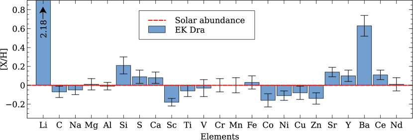
Figure 4: Logarithmic abundances of the elements for EK Dra relative to their solar abundances.

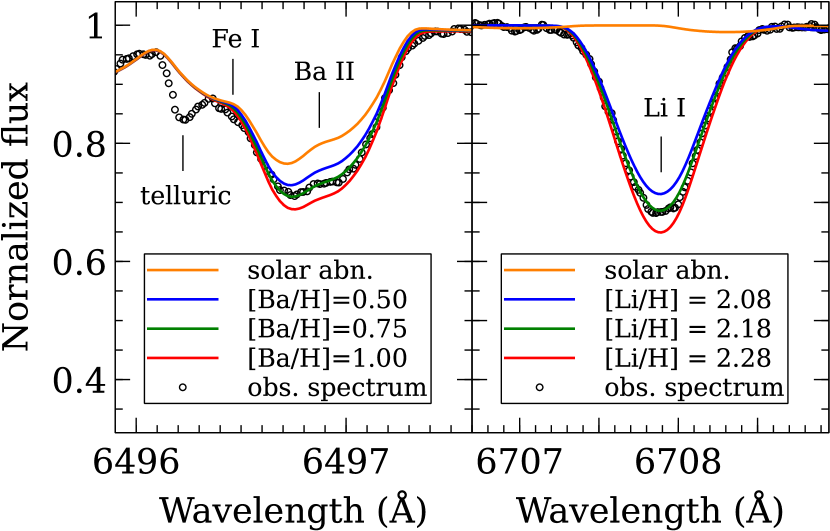
Figure 5: Ba II 6496.989 and L I 6707.983 lines yielding overabundances.

The lowest and highest values for the magnetic field $\langle B\rangle$ of EK Dra were reported as 57 and 92 G, respectively, by Waite et al. (2017). To test whether this magnetic field affects the derived chemical abundances, we plotted the abundances derived from individual lines with their effective Landé $g$ factors for Ti, Cr, Fe, and Ni (Fig. 6). Here, we note that we do not consider the change in the thermal properties of the stellar atmosphere introduce by magnetic fields (e.g., Solanki, 1986; Solanki & Brigljevic, 1992; Solanki, 1993), which can influence the strength of spectral lines irrespectively of their Landé $g$ factors (e.g., Solanki & Stenflo, 1984; Shelyag et al., 2007). We also note that the polarimetric estimates of $\langle B\rangle$ probably underestimate the actual values, because small-scale magnetic flux elements remain undetected. See et al. (2019), however, suggested that the level of underestimation may be minor for the specific case of EK Dra. Fig. 6 indicates the lines with larger Landé $g$ factors tend to give larger abundances, most-likely due to the magnetic strengthening of the absorption lines. This effect appears to be negligible for Ti and Fe with a Pearson Correlation Coefficient (PCC) of about 0.14 and the slopes of their regression lines are only 0.07 and 0.05, respectively. However, the effect is more noticeable for Cr, and particularly for Ni, with a larger PCCs of 0.29 and 0.45, and larger slopes of 0.15 and 0.24, respectively. This shows that our derived Cr snd Ni abundances might be slightly overestimated due to the magnetic field. Our test is restricted to only four chemical elements as the other elements do not provide sufficient number of modelable lines.

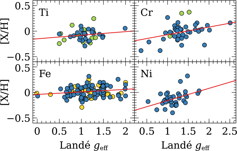
Figure 6: Line-by-line abundances of the elements versus effective Landé factors ($g_{\rm eff}$) of the lines. The abundances derived from the first and the second ionisation stages of the elements are represented by blue and green circles, respectively. For Fe, the yellow circles also represent Fe I, but they are for the lines with lower quality of oscillator strengths, i.e., quality of B+, B or worse in the accuracy classification of NIST.

5 The starspot distribution

5.1 Doppler Imaging

It is known that inaccurate stellar parameters lead to artefacts in the reconstructed Doppler images (e.g. Unruh, 1996). Optimal stellar parameters are thus crucial for DI reconstructions. Here, we take advantage of the fact that several DI reconstructions of EK Dra are available in the literature, providing us with a reliable set of initial parameters to use in our analysis. In this section, we first explain how we adopt the parameters obtained in this study (see Sections 3 and 4), and carry out a 2D grid search for the critical parameters used in the DI procedure.

We used the Doppler imaging code DoTS (Collier Cameron, 1997, 1992), which is based on the Maximum Entropy Method (MEM) for iterative regularisation of the resulting image. The DoTS code reconstructs the spot filling factor ($f_{s}$) across the observable part of the star, using a two-temperature approximation for the representation of the quiet photosphere and spotted pixels. This procedure requires look-up tables generated using spectra of template stars for the calculation of intensity contributions of each element across the stellar surface. We assumed the temperatures of the quiet and spotted photospheres as 5750 K and 5000 K, respectively, by adopting the average spot temperature from J18. We used the linear limb-darkening coefficients derived by Claret et al. (2012, 2013).

For the input stellar parameters required by the DoTS code, we used the ones obtained in Section 3, except for the axial inclination $i$ as $63^{\circ}$, the rotation period and the epoch as given in Equation 1, which we took from J18. In order to avoid spurious reconstruction of high-latitude spots, we performed a two-dimensional grid search for the equivalent-width parameter EW vs. $v\sin i$. The EW parameter controls the strength of the synthetic line profile. The resulting $\chi^{2}$ values are shown in Fig. 7. The $v\sin i$ value of 16.6$\pm 0.2$ km/s obtained from the grid search is in accordance with both J18 and the one based on the spectral synthesis in Sect. 3 (see Table 2). The error of the $v\sin i$ parameter was estimated from $\chi^{2}_{\rm min}+1$ of $v\sin i$ value obtained from two-dimensional grid search (see Bevington & Robinson, 2003, for details). Following MEM iterations, we achieved a reduced $\chi^{2}$ value of 1.127. In addition to the two-dimensional grid search for the EW and $v\sin i$ parameters (Fig. 7), we also carried out a grid search for the axial inclination (see Appendix A for details). Although the search result gives an axial inclination value of $56^{\circ}\pm 5^{\circ}$, we keep the value as $63^{\circ}$ during DI process for a more consistent comparison of the resultant map with the one obtained by J18 (see Section 5.2). The reconstructed spot positions and sizes do not alter significantly between inclination angles of $56$ and $63^{\circ}$.

The best-fit models for the velocity profiles obtained using the Calar-Alto dataset are given in Fig. 8, along with the residuals, which are within $\pm 0.0035$. The residuals are likely related to uncertainties in the estimation of stellar parameters. In order to examine the ${v\sin i}$ value that is obtained from $\chi^{2}$ minimisation, we also performed an alternative approach previously carried out by Donati et al. (2003) and recently by Cang et al. (2020), which is based on optimising the ${v\sin i}$ (and the EW parameter in our case) until phase-averaged residuals are minimised (see Appendix B for details). The resulting surface reconstructions (with the obtained $v\sin i$ of 16.6 km/s) are indistinguishable from our map in Fig. 8.

The projected disc images corresponding to the resulting Doppler image are shown in Fig. 9 at different rotational phases. The highest mean filling factor pertains to the spot near the pole, centred at around $77^{\circ}$ latitude. The remaining spots are distributed from middle to low latitudes. A detailed discussion on the spot distribution will be given in Sections 5.2 and 7.2.

Although Waite et al. (2017) did not find a measurable surface differential rotation using LSD intensity profiles, we ran a grid search to determine the differential rotation. We assumed

$$\Omega(\lambda)=\Omega_{\rm eq}-\Delta\Omega\sin^{2}\lambda,$$ (2)

where $\Omega$ is the angular velocity at a given latitude $\lambda$, $\Omega_{\rm eq}$ is that at the equator, and $\Delta\Omega$ is the pole-equator difference. We searched for the pair ($\Omega_{\rm eq}$, $\Delta\Omega$) that minimises $\chi^{2}$. The resulting $\chi^{2}$ landscape is shown in Fig. 10. The solutions did not converge to a global minimum, i.e., a reliable estimate for $\Delta\Omega$. Nevertheless, the deepest minimum lies within the range of strong shear rates estimated by Waite et al. (2017), using Stokes V data (about 4 times solar surface shear). It is also consistent with the shear derived from the range of photometric periods measured by Messina & Guinan (2003). Because our results do not provide a significant estimate for $\Delta\Omega$, we present the resulting sheared spot map only in the Appendix C. We have found that differential rotation of this magnitude mainly affects the shape of the spots, in the sense that spots appear more sheared, owing to latitudinal differential rotation. Also, less spots are reconstructed at low latitudes. To evaluate the effect of such strong surface shear levels on the surface reconstructions, we performed additional simulations using the FEAT model (see Section 6), of which further details are given in Appendix C.

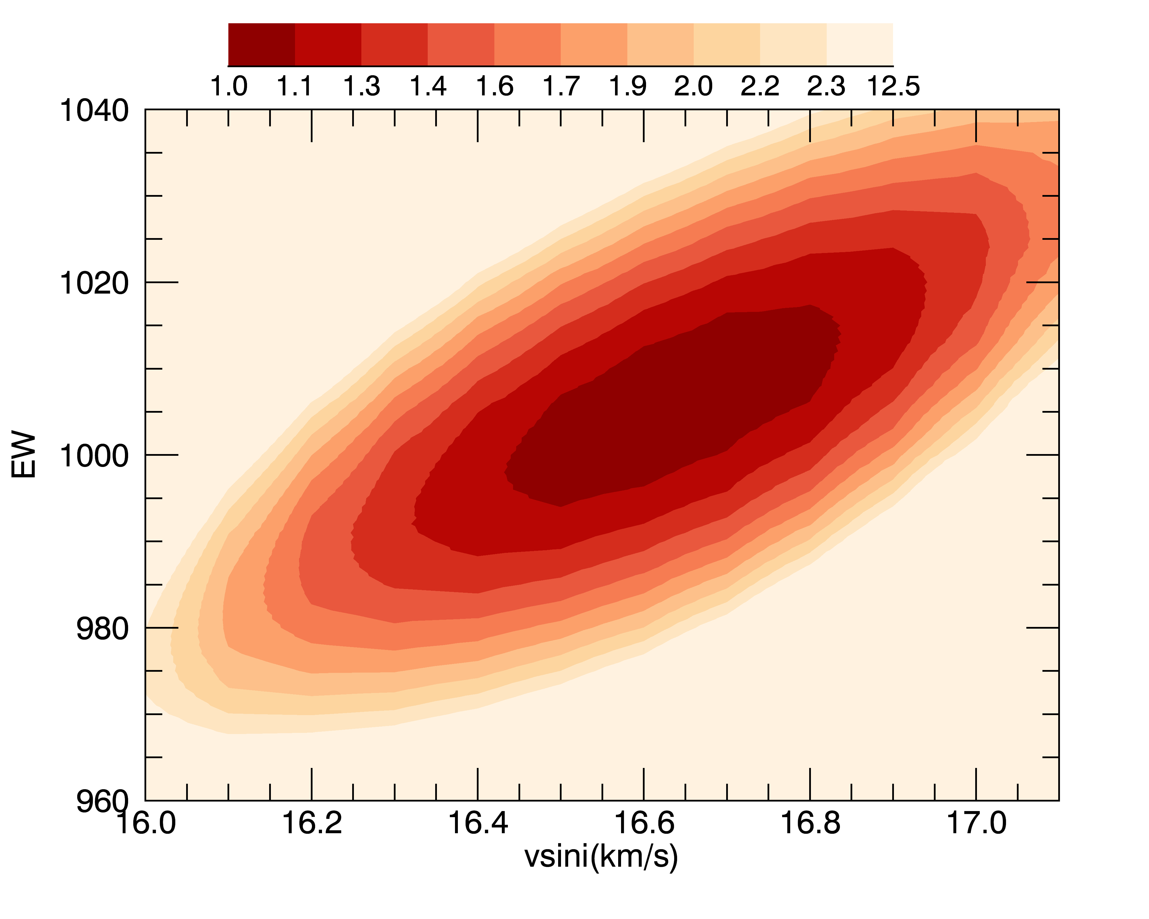
Figure 7: Two-dimensional grid search showing reduced $\chi^{2}$, used to optimise EW and ${v\sin i}$ parameters.

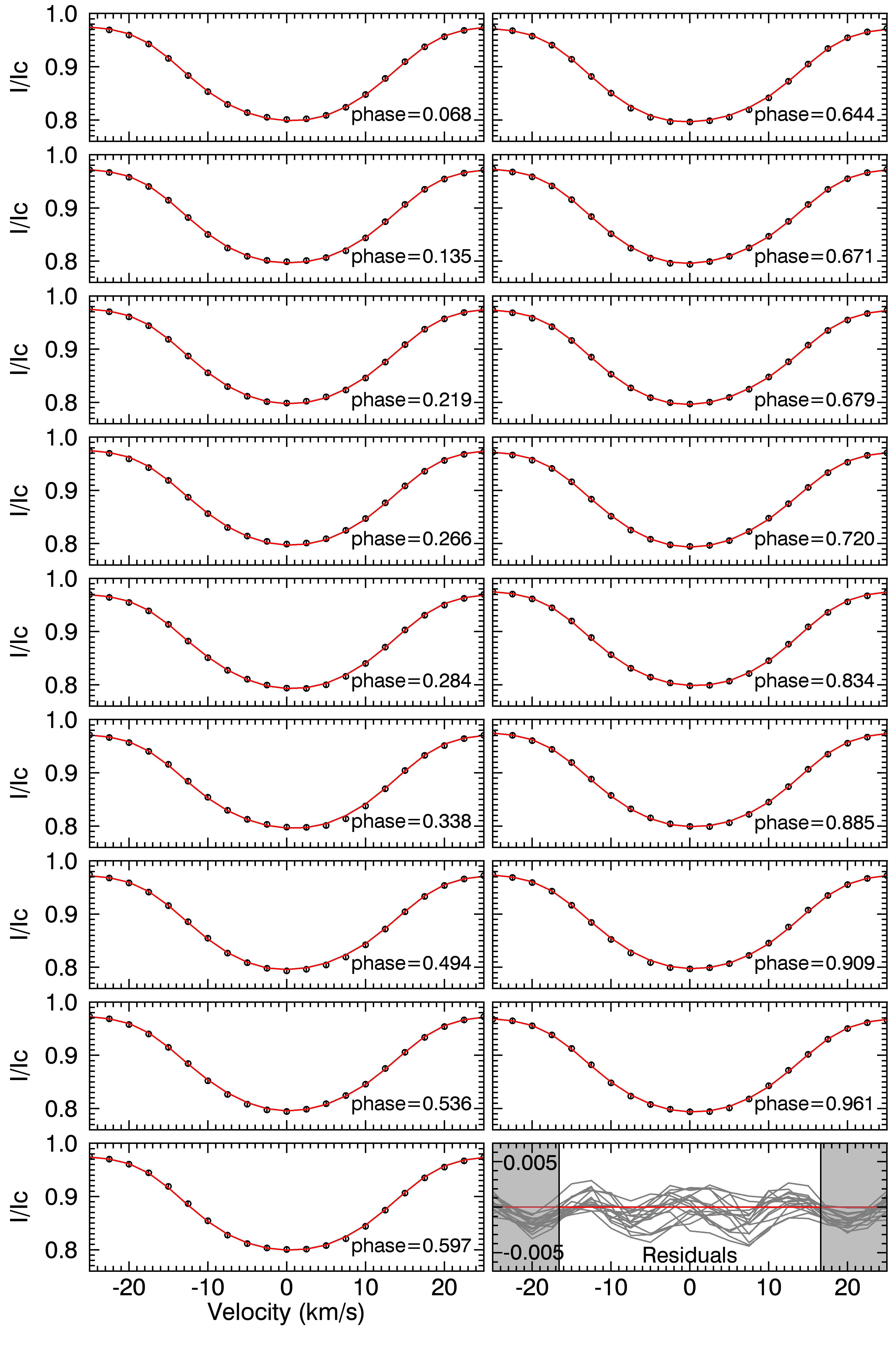
Figure 8: Phase-ordered LSD profiles (black circles). Red solid lines represent the maximum-entropy regularised models with the wavelength expressed in terms of radial velocity. The lowest-right panel shows the residuals of all observed profiles from the synthesised profiles, where the shaded regions mark the velocities beyond the $\pm v\sin i$ value. The rms value obtained from the combined residuals is $1.57\times 10^{-3}$ and $\chi^{2}=5.0\times 10^{-5}$. Note that the error bars of each data point remain inside the black circles.

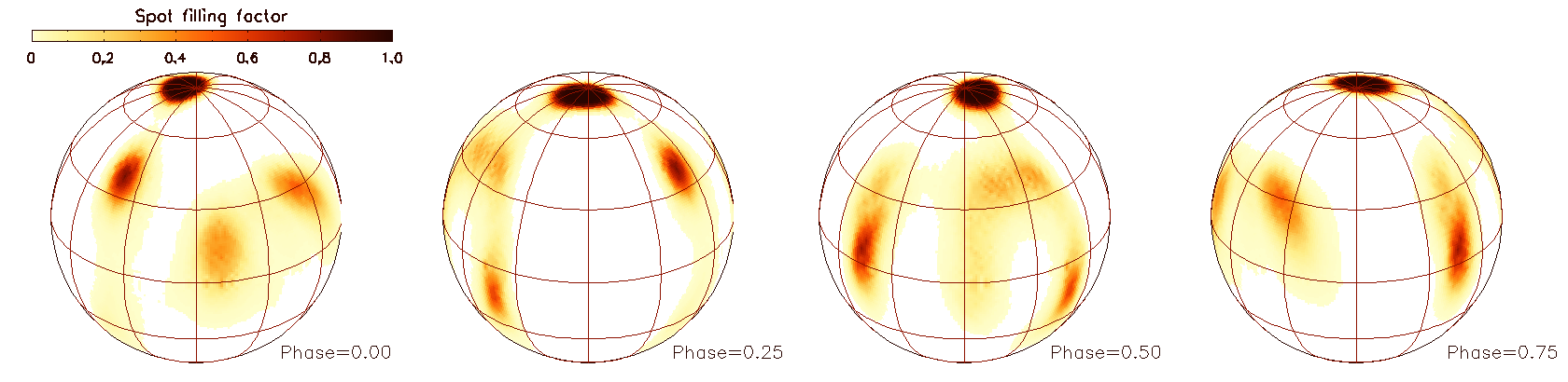
Figure 9: Projected disc images of EK Dra obtained from DI inversions at different rotational phases $\phi$=0.0, 0.25, 0.50, and 0.75.

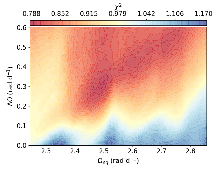
Figure 10: Two-dimensional grid search for the differential rotation parameters using Stokes I data of EK Draconis.

5.2 Comparing contemporaneous images

The most recent DI study of EK Dra was performed by J18, using very high resolution (R$\sim$230,000) spectral data, covering nine days. They obtained ten spectra between 3-11 April 2015, which is about 3.5 months earlier than our observations. This relatively short time interval between the observing runs provides an opportunity to compare the two maps. However, given the indications for strong differential rotation (Waite et al., 2017, and also our Fig. 10), a detailed comparison of spots between the two maps is likely unreliable, especially in the longitudinal direction. We emphasise that the following is a qualitative comparison between the overall spot distributions, in particular regarding the latitudinal zones where the spots are found.

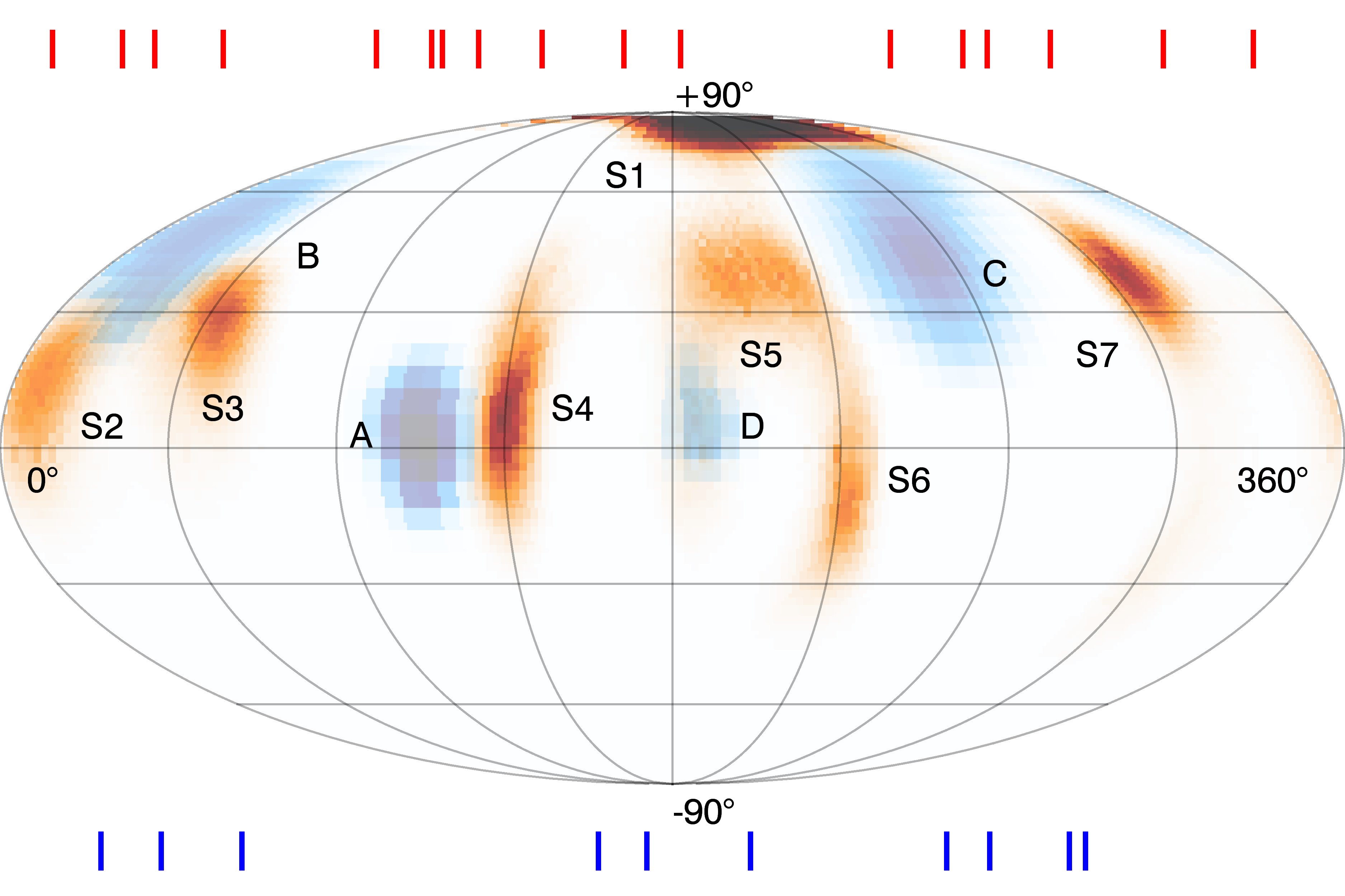
Figure 11: A comparison of the spot distribution of EK Dra obtained in this study (labelled as S1 to S5) and by Järvinen et al. (2018) (labelled as A to D). The red and blue stripes show the distribution of spectral data obtained in this study and by Järvinen et al. (2018) along stellar longitude.

We show in Fig. 11 a comparison of the two Doppler images, based on the same ephemeris, so that the rotational phases are congruent in both cases for the equator. Our near-polar spot S1 has no counterpart in the J18 image. However, both images show spots at mid-latitudes ($30^{\circ}$ to $60^{\circ}$, B-C vs. S3, S5, S7) and across the equator (A, D vs. S2, S4, S6). We suggest a possible explanation for the cross-equatorial spots in Section 7.2.

The occurrence of a strong near-polar spot in our map indicates a substantial change in the large-scale distribution of activity within 3.5 months. Such rapid variation was visible also in the surface maps by Waite et al. (2017), for December 2006, January and February 2007, as the high-latitude spot had disappeared within 3 months. In addition, their January 2008 map shows a predominant near-polar spot, which is very similar to the one in Fig. 9. The difference with the surface map obtained by J18 may indicate that we have captured an episode of polar-spot formation.

6 Modelling the spot distribution

We used the Flux Emergence And Transport (hereafter FEAT) modelling platform developed by Işık et al. (2018), to simulate the surface distribution of spotted regions on EK Dra. This platform consists of three parts: (1) a solar-like butterfly diagram of emergence latitudes, times, and sizes of spot groups through a single 11-year cycle; (2) the rise of magnetic flux loops from the base to the top of a solar-like convection zone model, which yields emergence latitudes and tilt angles; (3) surface transport of emerging magnetic flux in the form of bipolar magnetic regions (hereafter BMRs). The resulting time-dependent surface distribution of the signed magnetic field is then used to obtain the distribution of dark spots, using the simple approach taken by Işık et al. (2018): 1-degree-squared pixels with a field strength above 187 G is considered as pertaining to a starspot. This value was determined by matching the observed mean spot coverage on the Sun during a typical activity maximum, by taking into account pixels above this threshold in SFT snapshots.

In this way, we confront the simulated FEAT maps with the Doppler image obtained in Sect. 5. In this paper we do not give a full description of the FEAT model, for which we refer the reader to Işık et al. (2018). Before briefly describing the steps (1)-(3), we first assess the validity of adopting a solar internal structure model for EK Dra, when modelling the dynamics of flux tubes in step (2).

6.1 Convection zone geometry

We compare the convection zone geometry of a solar internal structure model with a corresponding model for EK Dra, using Modules for Experiments in Stellar Astrophysics (MESA Paxton et al., 2011; Paxton et al., 2013, 2015, 2018, 2019). Taking the initial mass to be $1.04\,M_{\odot}$ (Sect. 3, Table 2) and using the default parameters defined in MESA (as of this writing) with $Z=0.02$, we modelled the pre-main-sequence evolution of EK Dra. We also produced a reference model for the Sun at an age of $4.69$ Gyr.

Figure 12 shows the evolution of the base and the top locations of the convection zone from the MESA solution. The age and its error range indicated in the figure are taken from our estimate for EK Dra (Sect. 3). It turns out that the convection zone of EK Dra must have a very similar aspect ratio to that of the Sun. This result is consistent with our finding that EK Dra and the Sun are very close to each other in the $T_{\rm eff}-\log g$ diagram (Sect. 3, Fig. 1). Considering the proximity of EK Dra to the Sun on the $T_{\rm eff}-\log g$ diagram along with Fig. 12, we suggest that EK Dra has a more ’Sun-like’ internal stratification than that of a young $1\,M_{\odot}$ star at an age between 20-40 Myr! For this reason, we adopted the non-local mixing-length solar convection zone model when modelling the emergence of magnetic flux tubes (Sect. 6.2).

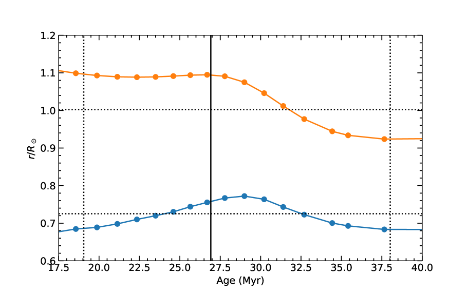
Figure 12: Evolution of the bottom (blue) and the top (orange) radial locations of the convection zone in a stellar model with the mass of EK Dra. The radial locations are given as fractions of the radius of a solar model at an age of 4.69 Gyr, for which the horizontal dotted lines show the convection zone boundaries. The vertical lines show EK Dra’s age (full line) and its error range (dotted lines).

6.2 Emergence and transport of magnetic flux

We carried out numerical simulations using the FEAT module for the emergence of magnetic flux. As in Işık et al. (2018), we set up a single activity cycle with a solar-like butterfly diagram at the bottom of the convection zone. The total number of emerging BMRs is scaled with the rotation rate with respect to that of the Sun, to account for the rotation-activity relation. EK Dra rotates at a rate of 9.6 times the Sun, so we assume its BMR emergence frequency is also 9.6 times that of the Sun throughout its activity cycle, which we simply assumed to be 11 years long. The models presented here are close to the model considered by Işık et al. (2018), for which the rotation rate and the activity level are 8 times that of the Sun.

Taking into account the solar convection-zone stratification (Sect. 6.1), we tracked the trajectories of magnetic flux tubes rising throughout the convection zone, for the rotation rate of EK Dra. For these computations we assumed that the internal rotation profile is the same as that of the Sun. The initial field strengths of the tubes were determined using a linear stability diagram for flux rings at the bottom of the convection zone, calculated for the rotation rate of EK Dra, using also a solar-like internal differential rotation profile with the solar absolute rotational shear.

As the final stage of FEAT, we carried out a surface flux transport (SFT) simulation covering 11 years of a solar-like cycle, for which the emergence latitudes and tilt angles were taken from the flux-tube simulations described above. We assumed the same latitudinal rotation profile as on the Sun, so that the pole-equator lag is the same as on the Sun. Two examples of the resulting surface images are shown in Fig. 13a,c, which are 3.5 months apart from each other, to evaluate possible extent of spot evolution within the time frame limited by our spectra and those of J18. To simulate the time spread of the spectra we used for DI, we averaged SFT snapshots with 1-day resolution over 15 days. The phase of the solar-like 11-year activity cycle shown here corresponds to about two years before the activity maximum. A near-polar spot region with a wide longitudinal extension is present, along with mid-latitude activity at smaller spatial scales. We note that each pixel on these images has an angular area of 1 degree-squared. The combined effect of mid-latitude emergence of strongly tilted BMRs, differential rotation, poleward meridional flow, and supergranular diffusion are responsible for the formation of the polar spot here (Schüssler et al., 1996; Schrijver & Title, 2001; Işık et al., 2007, 2011, 2018).

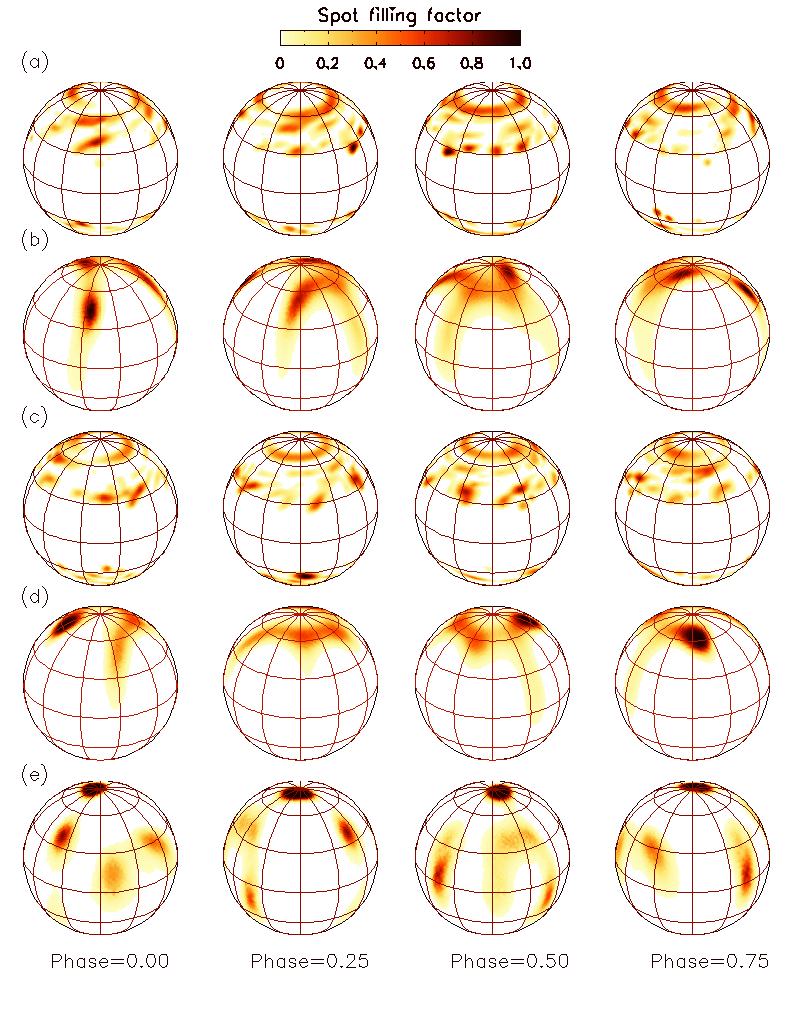
Figure 13: Comparison of FEAT simulations with the Doppler image of EK Dra. Panels (a) and (c) are 15-day averaged simulations as seen on four rotational phases, (b) and (d) show their corresponding synthetic Doppler images. Panel (e) shows the Doppler image (Fig. 9) reconstructed from the observations.

7 Discussion

7.1 Chemical composition

The effective temperature ($5770\pm 80$ K) and surface gravity ($\log g=4.4\pm 0.1$) we derived using various photometric and spectroscopic methods agree well with those derived by Strassmeier & Rice (1998); König et al. (2005); Järvinen et al. (2007, 2018) within the uncertainty limits. The derived microturbulent velocity, $\xi=1.7\pm 0.1$ km s^-1 agrees also well with that of Järvinen et al. (2007), which is 1.6 km s^-1, and it is slightly lower than that of Strassmeier & Rice (1998), which is 2.0 km s^-1. These atmospheric parameters are very similar to those of the Sun (Fig. 1).

We found the elemental abundances of the atmosphere of EK Dra to be nearly solar for all studied elements within $\pm 0.21$ deviation, except for Li and Ba (Fig. 4). The overabundance of [Li/H] = 2.18 indicates the youth of the star, i.e., $\tau\lesssim 50$ Myr, and is consistent with the age we found from the $T_{\rm eff}-{\rm log}g$ diagram ($27^{+11}_{-8}$ Myr). The Ba abundance was, however, most likely overestimated due to the assumption of depth-independent microturbulent velocity (see Reddy & Lambert, 2017). We estimate the corrected one as ${\rm[Ba/H]}\approx 0.18$. With this correction, the abundance pattern of EK Dra shows that Sr, Y, Ba, and Ce are marginally overabundant with respect to the Sun. The common trait of these four elements is that they are dominated by s-process nucleosynthesis for the solar system (see Fig. 20 of Wallerstein et al., 1997). The enrichment of these elements indicates that the progenitor low- and/or intermediate-mass AGB stars might have contributed the enrichment of EK Dra’s birthplace somewhat more than in the case of the solar nebula. The small but systematic underabundances of Co, Ni, Cu, and Zn indicate that supernovae have affected the birthplace of EK Dra to a lesser extent, in comparison to the pre-solar environment. However, we note that all such apparent abundance deviations of trace elements can result from the assumptions we used for the abundance analysis: the assumption of LTE, neglect of the 3D structure of the stellar photosphere, omission of magnetic field, and depth-independent microturbulent velocity. A more detailed 3D non-LTE atmosphere modelling can allow a more accurate assessment of the deviations from solar abundances in EK Dra’s atmosphere.

The position of EK Dra on the $T_{\mathrm{eff}}$-log $g$ diagram suggests that the star is on the pre-main-sequence with a mass of $1.04\pm 0.04$ M_⊙, most-likely being a post-T Tauri star. Montes et al. (2001) have mentioned that EK Dra is a member of the Local Association, using all three components of its space velocity. López-Santiago et al. (2006) also suggested that the star belongs to the Local Association B4 subgroup, using kinematic, spectroscopic, and photometric criteria. Using the Gaia DR2 data, we derived the space velocity components as $U=-5.98$ km s^-1, $V=-30.15$ km s^-1, and $W=-3.56$ km s^-1. In the $UV$ velocity plane, components match those typically measured in Pleiades cluster, subgroup B4, and AB Dor moving group. However, the estimated young age of the star is either smaller or at the lowest limit of these groups. This makes it difficult to clearly reveal which cluster/association/moving group the star belongs to. The W velocity component is also not close to any of those of these groups. The difference seen in the W component may be due to the radial velocity of the EK Dra being disturbed by the secondary component.

7.2 Spot distribution: observations vs. models

We now confront the FEAT simulations presented in Fig. 13a,c with the spot distribution inferred by Doppler imaging (Fig. 13e). To make them more compatible, we first rescaled the unsigned magnetic flux density (filtered between 187 and 800 G) to spot filling factor, so that any pixel with $|B|<187$ G has no contribution, and the pixel with $|B|\geqslant 800$ G has a filling factor of unity. Next, we generated synthetic LSD profiles at the same rotational phases as for our spectra. Using these profiles we produced two Doppler images corresponding to the two simulated epochs 3.5 months apart. This time interval was chosen to comply with the time difference between the spectra used by J18 and in this study (see Sect. 5.2, Fig. 11).

In the simulated DIs (Fig. 13b,d), it is evident that only relatively large structures were reconstructed. The main reason for this is that smaller individual spot groups do not distort the line profiles sufficiently to have detectable modulation. Another reason is that the maximum-entropy algorithm is sensitive to the largest gradients in the input image. There is a qualitative parallelism between the observed image and the simulated one in Fig. 13b, in that there is a strong near-polar and a mid-latitude (40-45^∘ latitude) feature of comparable contrast. There are no spots in the latitude range $0^{\circ}-30^{\circ}$ in the simulated Doppler images, unlike the observed DI. This is related to the relatively high lowest latitude, which is determined by the Coriolis effect imparted on rising flux tubes. For future modelling, we propose that a latitudinal scatter in emergence latitudes can be included in the model. This effect is already thought to occur in the Sun, owing to convective buffeting of rising tubes. An alternative (and perhaps co-existing) mechanism is that spot-producing flux tubes can form at any depth throughout the convection zone. Owing to a much shorter rising distance compared to that for the base of the convection zone, such tubes can be responsible for low-latitude spots. In some 3D magnetoconvection simulations, such toroidal flux systems are seen to self-organise in the midst of the convection zone (e.g. Nelson et al., 2013, 2014). These two effects, namely the latitudinal scatter and a more extended depth range for flux-tube formation, can be considered in the future as further improvements of the FEAT model.

In the simulations (compare Fig. 13a with b and c with d), the features which are extended over latitude down to the equator are signatures of mid-latitude spots in the southern hemisphere, which become prominent in some rotational phases. There are similar elongated features on the observed image, visible in all rotational phases, which can also be related to opposite-hemisphere spots. A prominent example is the spot that is highly extended to the southern hemisphere, centred at a negative latitude, near the rotational phase 0.35.

On the second simulated image (Fig. 13d), the similarity with the observed image is somewhat less, because the mean latitude of activity at this epoch (in the simulation) is closer to the pole, owing to poleward diffusion of highly tilted BMRs. For this reason, the strong southern feature in phase 0.25 in the input image does not lead to a large equatorward extension on the DI, but rather intensifies the high-latitude northern feature.

The SFT models in Fig. 13a,c show that within 3.5 months the spot configuration can change significantly, owing to a high emergence frequency of spots and the ongoing surface transport of magnetic flux. The resulting synthetic Doppler images (Fig. 13b,d) do not show much spatial correlation either. This means that any spatial correlation between the two Doppler images in Fig. 11 (especially in longitude) can be coincidental.

8 Conclusions

Based on the 23 elements analysed, we conclude that the chemical composition of EK Dra’s atmosphere is very similar to that of the Sun, within $\pm 0.21$ deviation, except for Li (Fig. 4). The excess of lithium is consistent with the age of the star, which we estimated to be $27^{+11}_{-8}$ Myr using isochrones on the $T_{\rm eff}-{\rm log}g$ diagram. This supports previous findings that EK Dra is a pre-main-sequence star in the post-T Tauri phase of its evolution. Its position on the HR diagram is so close to that of the Sun, that this 1.04-solar-mass star is closer to the Sun in terms of its internal structure than for a 1-solar-mass star of the same pre-main-sequence age.

Motivated by the first comparison of Doppler imaging and FEAT models, we conclude that the presence of near-polar and mid-latitude spots on Doppler images can be produced by a solar-type wave of activity in the convection zone, mediated by rotational effects on rising flux tubes (Schüssler & Solanki, 1992; Işık et al., 2018). However, the presence of near-equatorial spots are not fully explained by this model. We showed that at least those DI features with large latitudinal elongation can be contaminated by southern-hemisphere activity, which can be poorly reconstructed with the DI technique. The more compact and round features can be related with actual low-latitude emergence. In this case, convective buffeting of rising tubes or a radially extended generation of toroidal flux (i.e., a distributed dynamo) can be responsible. We suggest that when such low-latitude emergences are much less frequent than for mid-latitude emergences, they would be preferably detected with DI, which is sensitive to longitudinal gradients and works more precisely for lower latitudes, owing to the larger extent in radial velocities. Forward modelling of Doppler images with physical models (e.g., Lehmann et al., 2019, who modelled ZDI images) is promising for a deeper understanding of the observational manifestations of stellar activity patterns.

Appendix A axial inclination search

We carried out a grid search for the axial inclination parameter using the Calar-Alto dataset. The resulting variation of $\chi^{2}$ is shown in Fig. 14. We obtained the best axial inclination value as $56^{\circ}~{}\pm 5^{\circ}$ by fitting a parabola to $\chi^{2}$ values. Considering the formal error as $\pm 5^{\circ}$ and the systematic error to be higher, the resulting axial inclination value is consistent with the one obtained by J18, as well as the one by Waite et al. (2017). It is also consistent with the other stellar parameters (e.g., the stellar radius) reported in the literature. We also note that replacing $\i=63^{\circ}$ adopted in this study (Table 2) by $56^{\circ}$ has negligible impact on the reconstructed Doppler image.

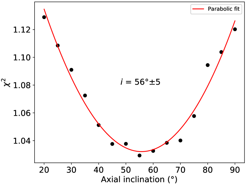
Figure 14: Results from a grid-search for the optimal axial inclination based on our data.

Appendix B Optimisation of projected rotational velocity and the equivalent width parameter

We have optimised $v\sin i$ by requiring that the phase-averaged residuals are minimised. This led to a $v\sin i$ of 16.7 km/s and a slightly higher EW than the estimate from Fig. 7. This solution is not far from that of $\chi^{2}$ minimisation, for which a $v\sin i$ of 16.6 km/s was found. The phase-averaged LSD profile, the model using the optimised parameters and the corresponding residuals are shown in Fig. 15. The morphology of the residuals is the same as that obtained for phase-ordered LSD profiles (lowest-right panel of Fig. 8). The residuals have an amplitude of about $\pm 0.001$, which is smaller than the residuals that were obtained by J18. The map reconstructed using the parameters achieved from the optimisation procedure is almost indifferent than the one imaged using parameters derived from $\chi^{2}$ minimisation.

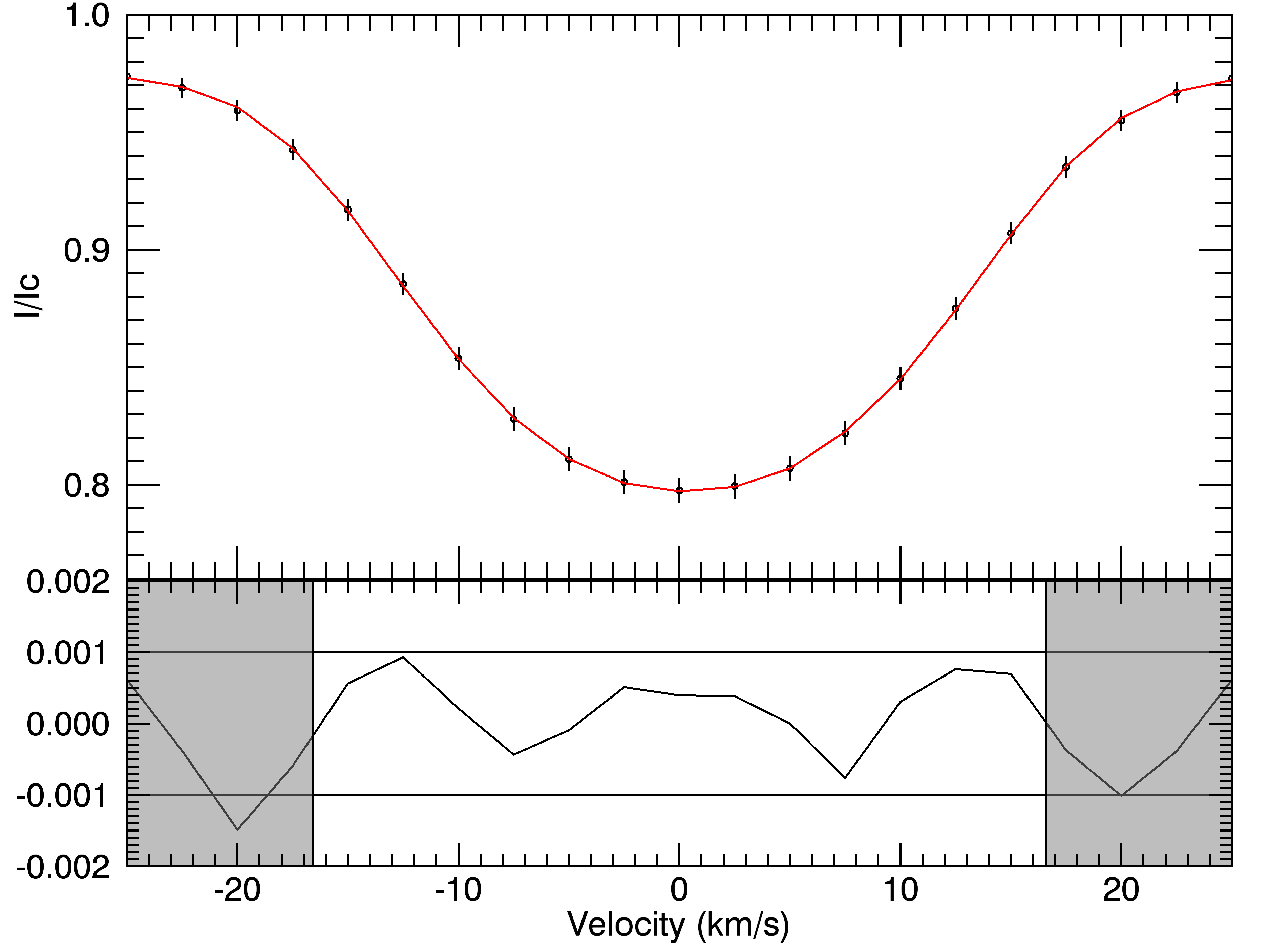
Figure 15: Phase-averaged LSD profile of EK Dra together with the error bars (top panel, black circles) obtained using the Calar-Alto data-set. Red solid line represents the maximum entropy regularised model obtained from the optimisation of the ${v\sin i}$ and the EW parameters. Bottom panel shows the residuals from the model.

Appendix C Simulations of strong differential rotation

There are multiple indications in the literature for the existence of strong solar-like differential rotation (DR) on EK Dra. Messina & Guinan (2003) used the observed range of photometric period from the observations covering $\sim$16 years and estimated an equator-to-pole difference in angular velocity, $\Delta\Omega$, of about 4 times the solar value. Based on 6 years of DR measurements with the ZDI technique, Waite et al. (2017, see Table 6) estimated a significantly large variance about the mean $\Delta\Omega=0.27$rad s^-1, which is also about 4 times solar DR. Because it is not possible to reach a global $\chi^{2}$ minimum for $\Delta\Omega$ and $\Omega$ using only the Stokes I (intensity) profiles (Fig. 10), we have presented the rigid-body-rotation solution in this study, as has been the standard approach in the field in such cases.

However, motivated by indications for strong DR on EK Dra, here we reconstructed DIs of SFT simulations that were run with 2 and 4 times solar DR ($\Delta\Omega$), in the same way as in Fig. 13a-d, which were for solar DR strength. The results are shown in Fig. 16 (panels A and B), where we imposed the corresponding DR strength. The longitudinal and latitudinal elongations of the spot features (owing to increasingly strong shear) follow similar patterns in the reconstructed maps. In addition, there are low-latitude spotted regions in the reconstructed maps, though no such features exist in the input SFT maps. This is a combined consequence of the higher resolving power of the DI technique at lower latitudes and the coincidental phase encounters of southern-hemisphere spots in the FEAT models, as discussed in Section 7.2. In general, there is reasonable agreement between the input images and the reconstructions, indicating that sheared spot distributions can be well-reconstructed for up to 4 times solar DR. For comparison, we show in Fig. 16 (panel C) two Doppler images of EK Dra, reconstructed for rigid rotation and for 4 times solar DR, which is about the value corresponding to the minimum $\chi^{2}$ in Fig. 10. In the sheared DI, there is considerably less spot coverage near the equator than in the rigid-body solution. In this sense, our FEAT models match more closely with the sheared DI of EK Dra.

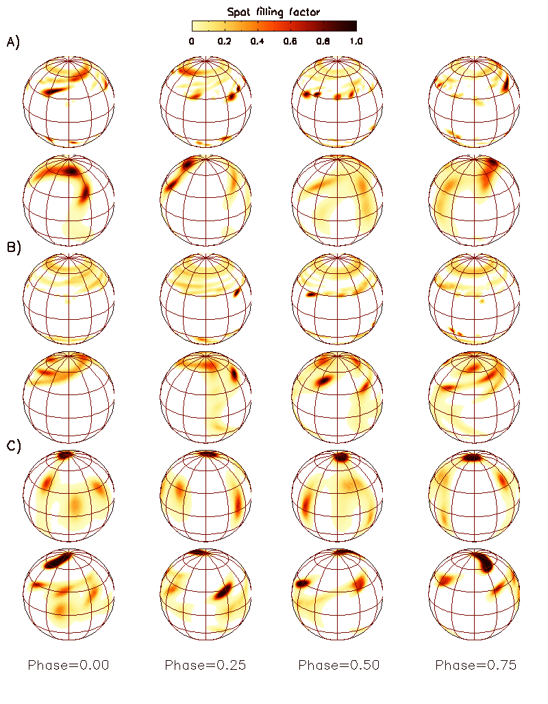
Figure 16: FEAT simulations and their reconstructions assuming 2 (panel A) and 4 (panel B) times the solar DR, in comparison to observed Doppler images of EK Dra for rigid-body and 4 times solar DR (panel C).

References

- Aceituno et al. (2013) Aceituno J., et al., 2013, A&A, 552, A31
- Aigrain et al. (2016) Aigrain S., et al., 2016, in 19th Cambridge Workshop on Cool Stars, Stellar Systems, and the Sun (CS19). p. 12, doi:10.5281/zenodo.154565
- Bessell et al. (1998) Bessell M. S., Castelli F., Plez B., 1998, A&A, 333, 231
- Bevington & Robinson (2003) Bevington P. R., Robinson D. K., 2003, Data reduction and error analysis for the physical sciences. Boston, MA: McGraw-Hill
- Boro Saikia et al. (2018) Boro Saikia S., et al., 2018, A&A, 616, A108
- Bressan et al. (2012) Bressan A., Marigo P., Girardi L., Salasnich B., Dal Cero C., Rubele S., Nanni A., 2012, MNRAS, 427, 127
- Brewer et al. (2016) Brewer J. M., Fischer D. A., Valenti J. A., Piskunov N., 2016, ApJS, 225, 32
- Brun & Browning (2017) Brun A. S., Browning M. K., 2017, Living Reviews in Solar Physics, 14, 4
- Cang et al. (2020) Cang T. Q., et al., 2020, arXiv e-prints, p. arXiv:2008.12120
- Carlos et al. (2016) Carlos M., Nissen P. E., Meléndez J., 2016, A&A, 587, A100
- Claret et al. (2012) Claret A., Hauschildt P. H., Witte S., 2012, A&A, 546, A14
- Claret et al. (2013) Claret A., Hauschildt P. H., Witte S., 2013, A&A, 552, A16
- Collier Cameron (1992) Collier Cameron A., 1992, in Byrne P. B., Mullan D. J., eds, Lecture Notes in Physics, Berlin Springer Verlag Vol. 397, Surface Inhomogeneities on Late-Type Stars. p. 33, doi:10.1007/3-540-55310-X_131
- Collier Cameron (1997) Collier Cameron A., 1997, MNRAS, 287, 556
- Donati et al. (1997) Donati J.-F., Semel M., Carter B. D., Rees D. E., Collier Cameron A., 1997, MNRAS, 291, 658
- Donati et al. (2003) Donati J. F., et al., 2003, MNRAS, 345, 1145
- ESA (1997) ESA ed. 1997, The HIPPARCOS and TYCHO catalogues. Astrometric and photometric star catalogues derived from the ESA HIPPARCOS Space Astrometry Mission ESA Special Publication Vol. 1200
- Flower (1996) Flower P. J., 1996, ApJ, 469, 355
- Fröhlich et al. (2002) Fröhlich H. E., Tschäpe R., Rüdiger G., Strassmeier K. G., 2002, A&A, 391, 659
- Gaia Collaboration et al. (2016) Gaia Collaboration et al., 2016, A&A, 595, A1
- Gaia Collaboration et al. (2018) Gaia Collaboration et al., 2018, A&A, 616, A1
- Green et al. (2015) Green G. M., et al., 2015, ApJ, 810, 25
- Grevesse & Sauval (1998) Grevesse N., Sauval A. J., 1998, Space Sci. Rev., 85, 161
- Güdel (2007) Güdel M., 2007, Living Reviews in Solar Physics, 4, 3
- Harutyunyan et al. (2018) Harutyunyan G., Steffen M., Mott A., Caffau E., Israelian G., González Hernández J. I., Strassmeier K. G., 2018, A&A, 618, A16
- Hauck & Mermilliod (1998) Hauck B., Mermilliod M., 1998, A&AS, 129, 431
- Işık et al. (2007) Işık E., Schüssler M., Solanki S. K., 2007, A&A, 464, 1049
- Işık et al. (2011) Işık E., Schmitt D., Schüssler M., 2011, A&A, 528, A135
- Işık et al. (2018) Işık E., Solanki S. K., Krivova N. A., Shapiro A. I., 2018, A&A, 620, A177
- Järvinen et al. (2005) Järvinen S. P., Berdyugina S. V., Strassmeier K. G., 2005, A&A, 440, 735
- Järvinen et al. (2007) Järvinen S. P., Berdyugina S. V., Korhonen H., Ilyin I., Tuominen I., 2007, A&A, 472, 887
- Järvinen et al. (2009) Järvinen S. P., Korhonen H., Berdyugina S. V., Ilyin I., 2009, in Stempels E., ed., American Institute of Physics Conference Series Vol. 1094, 15th Cambridge Workshop on Cool Stars, Stellar Systems, and the Sun. pp 660–663, doi:10.1063/1.3099200
- Järvinen et al. (2018) Järvinen S. P., Strassmeier K. G., Carroll T. A., Ilyin I., Weber M., 2018, A&A, 620, A162
- Johnstone (2017) Johnstone C. P., 2017, in Nandy D., Valio A., Petit P., eds, Vol. 328, Living Around Active Stars. pp 168–179, doi:10.1017/S1743921317003775
- Karoff et al. (2018) Karoff C., et al., 2018, ApJ, 852, 46
- Kılıçoğlu et al. (2016) Kılıçoğlu T., Monier R., Richer J., Fossati L., Albayrak B., 2016, AJ, 151, 49
- König et al. (2005) König B., Guenther E. W., Woitas J., Hatzes A. P., 2005, A&A, 435, 215
- Kramida et al. (2015) Kramida A., Yu. Ralchenko Reader J., and NIST ASD Team 2015, NIST Atomic Spectra Database (ver. 5.3), [Online]. Available: http://physics.nist.gov/asd [2017, October 1]. National Institute of Standards and Technology, Gaithersburg, MD.
- Kriskovics et al. (2019) Kriskovics L., Kővári Z., Vida K., Oláh K., Carroll T. A., Granzer T., 2019, A&A, 627, A52
- Kunzli et al. (1997) Kunzli M., North P., Kurucz R. L., Nicolet B., 1997, A&AS, 122, 51
- Kupka et al. (1999) Kupka F., Piskunov N., Ryabchikova T. A., Stempels H. C., Weiss W. W., 1999, A&AS, 138, 119
- Kupka et al. (2000) Kupka F. G., Ryabchikova T. A., Piskunov N. E., Stempels H. C., Weiss W. W., 2000, Baltic Astronomy, 9, 590
- Kurucz (1993) Kurucz R., 1993, ATLAS9 Stellar Atmosphere Programs and 2 km/s grid. Kurucz CD-ROM No. 13. Cambridge, Mass.: Smithsonian Astrophysical Observatory, 1993., 13
- Lehmann et al. (2019) Lehmann L. T., Hussain G. A. J., Jardine M. M., Mackay D. H., Vidotto A. A., 2019, MNRAS, 483, 5246
- López-Santiago et al. (2006) López-Santiago J., Montes D., Crespo-Chacón I., Fernández-Figueroa M. J., 2006, ApJ, 643, 1160
- Ludwig et al. (1999) Ludwig H.-G., Freytag B., Steffen M., 1999, A&A, 346, 111
- Markwardt (2009) Markwardt C. B., 2009, in Bohlender D. A., Durand D., Dowler P., eds, Astronomical Society of the Pacific Conference Series Vol. 411, Astronomical Data Analysis Software and Systems XVIII. p. 251 (arXiv:0902.2850)
- Martin et al. (1992) Martin E. L., Magazzu A., Rebolo R., 1992, A&A, 257, 186
- Messina & Guinan (2003) Messina S., Guinan E. F., 2003, A&A, 409, 1017
- Montes et al. (2001) Montes D., López-Santiago J., Fernández-Figueroa M. J., Gálvez M. C., 2001, A&A, 379, 976
- Napiwotzki (1997) Napiwotzki R., 1997, A&A, 322, 256
- Nelson et al. (2013) Nelson N. J., Brown B. P., Brun A. S., Miesch M. S., Toomre J., 2013, ApJ, 762, 73
- Nelson et al. (2014) Nelson N. J., Brown B. P., Brun A. S., Miesch M. S., Toomre J., 2014, Sol. Phys., 289, 441
- Olsen (1983) Olsen E. H., 1983, A&AS, 54, 55
- Paxton et al. (2011) Paxton B., Bildsten L., Dotter A., Herwig F., Lesaffre P., Timmes F., 2011, ApJS, 192, 3
- Paxton et al. (2013) Paxton B., et al., 2013, ApJS, 208, 4
- Paxton et al. (2015) Paxton B., et al., 2015, ApJS, 220, 15
- Paxton et al. (2018) Paxton B., et al., 2018, ApJS, 234, 34
- Paxton et al. (2019) Paxton B., et al., 2019, ApJS, 243, 10
- Piskunov et al. (1995) Piskunov N. E., Kupka F., Ryabchikova T. A., Weiss W. W., Jeffery C. S., 1995, A&AS, 112, 525
- Raskin et al. (2011) Raskin G., et al., 2011, A&A, 526, A69
- Reddy & Lambert (2017) Reddy A. B. S., Lambert D. L., 2017, ApJ, 845, 151
- Reddy et al. (2002) Reddy B. E., Lambert D. L., Laws C., Gonzalez G., Covey K., 2002, MNRAS, 335, 1005
- Rosén et al. (2016) Rosén L., Kochukhov O., Hackman T., Lehtinen J., 2016, A&A, 593, A35
- Rufener (1988) Rufener F., 1988, Catalogue of stars measured in the Geneva Observatory photometric system : 4 : 1988
- Ryabchikova et al. (1997) Ryabchikova T. A., Piskunov N. E., Kupka F., Weiss W. W., 1997, Baltic Astronomy, 6, 244
- Sbordone et al. (2004) Sbordone L., Bonifacio P., Castelli F., Kurucz R. L., 2004, Memorie della Societa Astronomica Italiana Supplementi, 5, 93
- Schrijver & Title (2001) Schrijver C. J., Title A. M., 2001, ApJ, 551, 1099
- Schüssler & Solanki (1992) Schüssler M., Solanki S. K., 1992, A&A, 264, L13
- Schüssler et al. (1996) Schüssler M., Caligari P., Ferriz-Mas A., Solanki S. K., Stix M., 1996, A&A, 314, 503
- See et al. (2019) See V., et al., 2019, ApJ, 876, 118
- Sekiguchi & Fukugita (2000) Sekiguchi M., Fukugita M., 2000, AJ, 120, 1072
- Shelyag et al. (2007) Shelyag S., Schüssler M., Solanki S. K., Vögler A., 2007, A&A, 469, 731
- Soderblom & Clements (1987) Soderblom D. R., Clements S. D., 1987, AJ, 93, 920
- Solanki (1986) Solanki S. K., 1986, A&A, 168, 311
- Solanki (1993) Solanki S. K., 1993, Space Sci. Rev., 63, 1
- Solanki & Brigljevic (1992) Solanki S. K., Brigljevic V., 1992, A&A, 262, L29
- Solanki & Stenflo (1984) Solanki S. K., Stenflo J. O., 1984, A&A, 140, 185
- Stauffer et al. (1998) Stauffer J. R., Schultz G., Kirkpatrick J. D., 1998, ApJ, 499, L199
- Strassmeier (2009) Strassmeier K. G., 2009, A&ARv, 17, 251
- Strassmeier & Rice (1998) Strassmeier K. G., Rice J. B., 1998, A&A, 330, 685
- Unruh (1996) Unruh Y. C., 1996, in Strassmeier K. G., Linsky J. L., eds, IAU Symposium Vol. 176, Stellar Surface Structure. p. 35
- Valenti & Fischer (2005) Valenti J. A., Fischer D. A., 2005, ApJS, 159, 141
- Waite et al. (2017) Waite I. A., et al., 2017, MNRAS, 465, 2076
- Wallerstein et al. (1997) Wallerstein G., et al., 1997, Reviews of Modern Physics, 69, 995
- Weiler (2018) Weiler M., 2018, A&A, 617, A138
- Wichmann et al. (2003) Wichmann R., Schmitt J. H. M. M., Hubrig S., 2003, A&A, 399, 983