Multimodal Variational Autoencoders for Semi-Supervised Learning: In Defense of Product-of-Experts

Abstract

Multimodal generative models should be able to learn a meaningful latent representation that enables a coherent joint generation of all modalities (e.g., images and text). Many applications also require the ability to accurately sample modalities conditioned on observations of a subset of the modalities. Often not all modalities may be observed for all training data points, so semi-supervised learning should be possible. In this study, we propose a novel product-of-experts (PoE) based variational autoencoder that have these desired properties. We benchmark it against a mixture-of-experts (MoE) approach and a PoE approach of combining the modalities with an additional encoder network. An empirical evaluation shows that the PoE based models can outperform the contrasted models. Our experiments support the intuition that PoE models are more suited for a conjunctive combination of modalities.

[inst1]organization=Novo Nordisk Foundation Center for Biosustainability, Technical University of Denmark, addressline=Kemitorvet 220, city=Copenhagen, postcode=2800, country=Denmark

[inst2]organization=Department of Computer Science, University of Copenhagen, addressline=Universitetsparken 1, city=Copenhagen, postcode=2100, country=Denmark

1 Introduction

Multimodal generative modelling is important because information about real-world objects typically comes in different representations, or modalities. The information provided by each modality may be erroneous and/or incomplete, and a complete reconstruction of the full information can often only be achieved by combining several modalities. For example, in image- and video-guided translation [1], additional visual context can potentially resolve ambiguities (e.g., noun genders) when translating written text.

In many applications, modalities may be missing for a subset of the observed samples during training and deployment. Often the description of an object in one modality is easy to obtain, while annotating it with another modality is slow and expensive. Given two modalities, we call samples paired when both modalities are present, and unpaired if one is missing. The simplest way to deal with paired and unpaired training examples is to discard the unpaired observations for learning. The smaller the share of paired samples, the more important becomes the ability to additionally learn from the unpaired data, referred to as semi-supervised learning in this context (following the terminology from 2. Typically one would associate semi-supervised learning with learning form labelled and unlabelled data to solve a classification or regression tasks). Our goal is to provide a model that can leverage the information contained in unpaired samples and to investigate the capabilities of the model in situations of low levels of supervision, that is, when only a few paired samples are available. While a modality can be as low dimensional as a label, which can be handled by a variety of discriminative models [3], we are interested in high dimensional modalities, for example an image and a text caption.

Learning a representation of multimodal data that allows to generate high-quality samples requires the following: 1) deriving a meaningful representation in a joint latent space for each high dimensional modality and 2) bridging the representations of different modalities in a way that the relations between them are preserved. The latter means that we do not want the modalities to be represented orthogonally in the latent space – ideally the latent space should encode the object’s properties independent of the input modality. Variational autoencoders (4) using a product-of-experts (PoE, 5, 6) approach for combining input modalities are a promising approach for multimodal generative modelling having the desired properties, in particular the VAEVAE(a) model developed by [7] and a novel model termed SVAE, which we present in this study. Both models can handle multiple high dimensional modalities, which may not all be observed at training time.

It has been argued that a PoE approach is not well suited for multimodal generative modelling using variational autoencoders (VAEs) in comparison to additive mixture-of-experts (MoE). It has empirically been shown that the PoE-based MVAE [7] fails to properly model two high-dimensional modalities in contrast to an (additive) MoE approach referred to as MMVAE, leading to the conclusion that “PoE factorisation does not appear to be practically suited for multi-modal learning” [8]. This study sets out to test this conjecture for state-of-the-art multimodal VAEs.

The next section summarizes related work. Section 3 introduces SVAE as an alternative PoE based VAE approach derived from axiomatic principles. Then we present our experimental evaluation of multimodal VAEs before we conclude.

2 Background and Related Work

We consider multimodal generative modelling. We mainly restrict our considerations to two modalities $x_{1}\in X_{1},x_{2}\in X_{2}$, where one modality may be missing at a time. Extensions to more modalities are discussed in Section 3.5. To address the problem of generative cross-modal modeling, one modality $x_{1}$ can be generated from another modality $x_{2}$ by simply using independently trained generative models ($x_{1}\rightarrow x_{2}$ and $x_{2}\rightarrow x_{1}$) or a composed but non-interchangeable representation [9, 10]. However, the ultimate goal of multimodal representation learning is to find a meaningful joint latent code distribution bridging the two individual embeddings learned from $x_{1}$ and $x_{2}$ alone. This can be done by a two-step procedure that models the individual representations first and then applies an additional learning step to link them [11, 12, 13]. In contrast, we focus on approaches that learn individual and joint representations simultaneously. Furthermore, our model should be able to learn in a semi-supervised setting. [14] introduced two models suitable for the case when one modality is high dimensional (e.g., an image) and another is low dimensional (e.g., a label) while our main interest are modalities of high complexity.

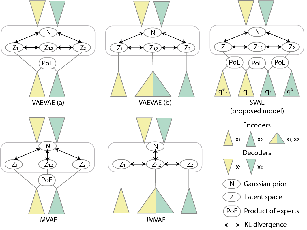
Figure 1: Schematic overview bi-modal VAEs using a PoE and additional network structures that are capable of semi-supervised learning without requiring a two step learning procedure. VAEVAE (a) and (b) are by [2], JMVAE is by [15], MVAE is by [7], and SVAE is our newly proposed model. Each triangle stands for an individual neural network, the colors indicate the two different modalities.

We consider models based on variational autoencoders (VAEs, 4, 16). Standard VAEs learn a latent representation $z\in Z$ for a set of observed variables $x\in X$ by modelling a joint distribution $p(x,z)=p(z)p(x|z)$. In the original VAE, the intractable posterior $q(z|x)$ and conditional distribution $p(x|z)$ are approximated by neural networks trained by maximising the ELBO loss taking the form

$$\mathcal{L}=E_{q(z|x)}[\log{p(x|z)}]-D_{\text{KL}}(q(z|x)\;\|\;\mathcal{N}(0,I))$$ (1)

with respect to the parameters of the networks modelling $q(z|x)$ and $p(x|z)$. Here $D_{\text{KL}}(\cdot\;\|\;\cdot)$ denotes the Kullback-Leibler divergence. Bi-modal VAEs that can handle a missing modality extend this approach by modelling $q(z|x_{1},x_{2})$ as well as $q_{1}(z|x_{1})$ and $q_{2}(z|x_{2})$, which replace the single $q(z|x)$. Multimodal VAEs may differ in 1) the way they approximate $q(z|x_{1},x_{2})$, $q_{1}(z|x_{1})$ and $q_{2}(z|x_{2})$ by neural networks and/or 2) the structure of the loss function, see Figure 1. Typically, there are no conceptual differences in the decoding, and we model the decoding distributions in the same way for all methods considered in this study.

[15] introduced a model termed JMVAE (Joint Multimodal VAE), which belongs to the class of approaches that can only learn from the paired training samples (what we refer to as the (fully) supervised setting). It approximates $q(z|x_{1},x_{2})$, $q_{1}(z|x_{1})$ and $q_{2}(z|x_{2})$ with three corresponding neural networks and optimizes an ELBO-type loss of the form

$$\mathcal{L}=E_{q(z|x_{1},x_{2})}[\log{p_{1}(x_{1}|z)}+\log{p_{2}(x_{2}|z)}]-D_{\text{KL}}(q(z|x_{1},x_{2})\;\|\;\mathcal{N}(0,I))\\ -D_{\text{KL}}(q(z|x_{1},x_{2})\;\|\;q_{1}(z|x_{1}))-D_{\text{KL}}(q(z|x_{1},x_{2})\;\|\;q_{2}(z|x_{2}))\enspace.$$ (2)

The last two terms imply that during learning the joint network output must be generated which requires paired samples.

The MVAE (Multimodal VAE) model [7] is the first multimodal VAE-based model allowing for missing modalities that does not require any additional network structures for learning the joint latent code distribution. The joint posterior is modeled using a product-of-experts (PoE, 5, 6) as $q(z|x_{1:M})\propto\prod_{m}q_{m}(z|x_{m})$. For the missing modality $q_{k}(z|x_{k})=1$ is assumed. The model by [7] allows for semi-supervised learning while keeping the number of model parameters low. The multiplicative combination of the experts can be interpreted as a conjunction. In the context of probabilistic metric spaces, the product is a triangular norm (t-norm) and generalizes the “AND” operation to multi-valued logic.

The bridged model [17] highlights the need for an additional network structure for approximating the joint latent code distribution. It attempts to keep the advantages of the additional encoding networks. It reduces the number of model parameters by introducing the bridge encoder that consists of one fully connected layer which takes $z_{1}$ and $z_{2}$ latent code vectors generated from $x_{1}$ and $x_{2}$ and outputs the mean and the variance of the joint latent code distribution.

The arguably most advanced multimodal VAE models is VAEVAE by [2], which we discuss in detail in the next section (see also Algorithm 1).

[8] proposed a MoE model termed MMVAE (Mixture-of-experts Multimodal VAE). In MMVAE model the joint variational posterior for $M$ modalities is approximated as $q(z|x_{1:M})=\sum_{m}{\alpha_{m}}q_{m}(z|x_{m})$ where $\alpha_{m}=\frac{1}{M}$. The model utilizes a loss function from the importance weighted autoencoder (IWAE, 18) that computes a tighter lower bound compared to the VAE ELBO loss. The MoE rule formulation allows in principle to train with a missing modality $i$ by assuming $\alpha_{i}=0$, however, [8] do not highlight or evaluate this feature. They empirically compare MVAE [7] and MMVAE, concluding that MVAE often fails to learn the joint latent code distribution. Because of these results and those presented by [2], we did not include MVAE as a benchmark model in our experiments.

3 SVAE

We developed a new approach as an alternative to VAEVAE. Both models 1) are VAE based; 2) allow for interchangeable cross-model generation as well as a learning joint embedding; 3) allow for missing modalities at training time; and 4) can be applied to two similarly complex high dimensional modalities. Next, we will present our new model SVAE (it was originally developed to analyse mass spectrometry data, see Section 4.4, and thus referred to as SpectraVAE). Then we highlight the differences to VAEVAE. Finally, we state a newly derived objective function for training the models. We first consider two modalities and generalize to more modalities in Section 3.5.

3.1 SVAE

Since both modalities might not be available for all the samples, it should be possible to marginalize each of them out of $q(z|x_{1},x_{2})$. While the individual encoding distributions $q(z|x_{1})$ and $q(z|x_{2})$ can be approximated by neural networks as in the standard VAE, we need to define a meaningful approximation of the joint encoding distribution $q(z|x)=q(z|x_{1},x_{2})$. In the newly proposed SVAE model, these distributions are defined as the following:

$$q(z|x_{1},x_{2}) =\frac{1}{Z(x_{1},x_{2})}q_{1}(z|x_{1})q_{2}(z|x_{2})$$ (3)

$$q(z|x_{1}) =q_{1}(z|x_{1})q^{*}_{2}(z|x_{1})$$ (4)

$$q(z|x_{2}) =q_{2}(z|x_{2})q^{*}_{1}(z|x_{2})$$ (5)

$$q(z) =\mathcal{N}(0,I)$$ (6)

where $Z(x_{1},x_{2})$ is a normalization constant. The distributions $q_{1}(z|x_{1})$, $q_{2}(z|x_{2})$ and the unormalized distributions $q^{*}_{2}(z|x_{1})$ and $q^{*}_{1}(z|x_{2})$ are approximated by different neural networks. The networks approximating $q_{i}(z|x_{i})$ and $q^{*}_{j}(z|x_{i})$, $i,j\in\{1,2\}$ have the same architecture. In case both observations are available, $q(z|x_{1},x_{2})$ is approximated by applying the product-of-experts rule with $q_{1}(z|x_{1})$ and $q_{2}(z|x_{2})$ being the experts for each modality. In case of a missing modality, equation 4 or 5 is used. If, for example, $x_{2}$ is missing, the $q^{*}_{2}(z|x_{1})$ distribution takes over as a “replacement” expert, modelling marginalization over $x_{2}$.

The model is derived in Section 3.2. The desired properties of the model were that 1) when no modalities are observed the generating distribution for the latent code is Gaussian, 2) the modalities are independent given the latent code, 3) both experts cover the whole latent space with equal probabilities, and 4) the joint encoding distribution $q(z|x_{1},x_{2})$ is modelled by a PoE.

3.2 Derivation of the SVAE model architecture

We define our model in an axiomatic way, requiring the following properties:

1. When no modalities are observed, the generating distribution for the latent code is Gaussian:

   $$q(z)=p(z)=\mathcal{N}(0,I)$$ (7)

   This property is well known from VAEs and allows easy sampling.

2. The two modalities are independent given the latent code, so the decoder distribution is:

   $$p(x_{1},x_{2}|z)=p_{1}(x_{1}|z)p_{2}(x_{2}|z)$$ (8)

   The second property formalizes our goal that the latent representation contains all relevant information from all modalities.

   The joint distribution $p(z|x)=p(z|x_{1},x_{2})$ is given by

   $$p(z|x_{1},x_{2})=\frac{p(z)p_{1}(x_{1},x_{2}|z)}{p(x_{1},x_{2})}=\frac{p(z)p_{1}(x_{1},x_{2}|z)}{\int p(z^{\prime})p(x_{1},x_{2}|z^{\prime})\text{d}z^{\prime}}\\ \overset{(\ref{eqa})}{=}\frac{p(z)p_{1}(x_{1}|z)p_{2}(x_{2}|z)}{\int p(z^{\prime})p(x_{1}|z^{\prime})p(x_{2}|z^{\prime})\text{d}z^{\prime}}\enspace.$$ (9)

3. Both experts cover the whole latent space with equal probabilities:

   $$q(z)=q_{1}(z)=\int q_{1}(z|x_{1})p(x_{1})\text{d}x_{1}=\int q_{2}(z|x_{2})p(x_{2})\text{d}x_{2}=q_{2}(z)$$ (10)

4. The joint encoding distribution $q(z|x)=q(z|x_{1},x_{2})$ is assumed to be given by the product-of-experts rule [5, 6]:

   $$q(z|x_{1},x_{2})=\frac{1}{Z(x_{1},x_{2})}q_{1}(z|x_{1})q_{2}(z|x_{2})$$ (11)

   with $Z(x_{1},x_{2})=\int q_{1}(z^{\prime}|x_{1})q_{2}(z^{\prime}|x_{2})\text{d}z^{\prime}$. The modelling by a product-of-experts in equation 11 is a simplification of equation 9 to make the model tractable.

Given equation 11 and equation 10 we obtain

$$q(z)=\int q(z|x)p(x)\text{d}x=\int q(z|x_{1},x_{2})p(x_{1},x_{2})\text{d}x_{1}\text{d}x_{2}\\ \overset{(\ref{eq2})}{=}\int\frac{1}{Z(x_{1},x_{2})}q_{1}(z|x_{1})q_{2}(z|x_{2})p(x_{1})p(x_{2}|x_{1})\text{d}x_{1}\text{d}x_{2}\enspace.$$ (12)

Let us define

$$q^{*}_{j}(z|x_{i})=\int\frac{1}{Z(x_{i},x_{j})}q_{j}(z|x_{j})p(x_{j}|x_{i})\text{d}x_{j}$$ (13)

and write

$$q(z)\overset{(\ref{eq5})}{=}\int q_{1}(z|x_{1})p(x_{1})\int\frac{1}{Z(x_{1},x_{2})}q_{2}(z|x_{2})p(x_{2}|x_{1})\text{d}x_{2}\text{d}x_{1}\\ =\int p(x_{1})q_{1}(z|x_{1})q^{*}_{2}(z|x_{1})\text{d}x_{1}\enspace.$$ (14)

So the proposal distributions are:

$$q(z|x_{1},x_{2}) =\frac{1}{Z(x_{1},x_{2})}q_{1}(z|x_{1})q_{2}(z|x_{2})$$ (15)

$$q(z|x_{1}) =q_{1}(z|x_{1})q^{*}_{2}(z|x_{1})$$ (16)

$$q(z|x_{2}) =q_{2}(z|x_{2})q^{*}_{1}(z|x_{2})$$ (17)

$$q(z) =\mathcal{N}(0,I)$$ (18)

3.3 SVAE vs. VAEVAE

The VAEVAE model [2] is the most similar to ours. Wu et al. define two variants which can be derived from the SVAE model in the following way. Variant (a) can be derived by setting $q^{*}(z|x_{1})=q^{*}(z|x_{2})=1$. Variant (b) is obtained from (a) by additionally using a separate network to model $q(z|x_{1},x_{2})$. Having a joint network $q(z|x_{1},x_{2})$ implements the most straightforward way of capturing the inter-dependencies of the two modalities. However, the joint network cannot be trained on unpaired data – which can be relevant when the share of supervised data gets smaller. Option (a) uses the product-of-experts rule to model the joint distribution of the two modalities as well, but does not ensure that both experts cover the whole latent space (in contrast to SVAE, see equation 10), which can lead to individual latent code distributions diverging. Based on this consideration and the experimental results from [2], we focused on benchmarking VAEVAE (b) and refer to it as simply VAEVAE in Section 4.

SVAE resembles VAEVAE in the need for additional networks besides one encoder per each modality and the structure of ELBO loss. It does, however, solve the problem of learning the joint embeddings in a way that allows to learn the parameters of approximated $q(z|x_{1},x_{2})$ using all available samples, i.e., both paired and unpaired. If $q(z|x_{1},x_{2})$ is approximated with the joint network that accepts concatenated inputs, as in JMVAE and VAEVAE (b), the weights of $q(z|x_{1},x_{2})$ can only be updated for the paired share of samples. If $q(z|x_{1},x_{2})$ is approximated with a PoE of decoupled networks as in SVAE, the weights are updated for each sample whether paired or unpaired – which is the key differentiating feature of SVAE compared to existing architectures.

3.4 A New Objective Function

When developing SVAE, we devised a novel ELBO-type loss:

$$\mathcal{L}= E_{p_{\text{paired}}(x_{1},x_{2})}\big{[}E_{q(z|x_{1},x_{2})}[\log{p_{1}(x_{1}|z)}+\log{p_{2}(x_{2}|z)}]$$

$$-D_{\text{KL}}(q(z|x_{1},x_{2})\;\|\;p(z|x_{1}))-D_{\text{KL}}(q(z|x_{1},x_{2})\;\|\;p(z|x_{2}))\big{]}$$

$$+E_{p_{\text{paired}}(x_{1})}\left[E_{q(z|x_{1})}[\log{p_{1}(x_{1}|z)}]-D_{\text{KL}}(q(z|x_{1})\;\|\;p(z))\right]$$

$$+E_{p_{\text{paired}}(x_{2})}\left[E_{q(z|x_{2})}[\log{p_{2}(x_{2}|z)}]-D_{\text{KL}}(q(z|x_{2})\;\|\;p(z))\right]$$ (19)

$$\mathcal{L}_{1}= E_{p_{\text{unpaired}}(x_{1})}\left[E_{q(z|x_{1})}[\log{p_{1}(x_{1}|z)}]-D_{\text{KL}}(q(z|x_{1})\;\|\;p(z))\right]$$ (20)

$$\mathcal{L}_{2}= E_{p_{\text{unpaired}}(x_{2})}\left[E_{q(z|x_{2})}[\log{p_{2}(x_{2}|z)}]-D_{\text{KL}}(q(z|x_{2})\;\|\;p(z))\right]$$ (21)

$$\mathcal{L}_{\text{comb}}= \mathcal{L}+\mathcal{L}_{1}+\mathcal{L}_{2}$$ (22)

Here $p_{\text{paired}}$ and $p_{\text{unpaired}}$ denote the distributions of the paired and unpaired training data, respectively. The differences between this loss and the loss function used to train VAEVAE by [2] are highlighted in Algorithm 1.

The loss function can derived as follows. Let consider the optimization problem

$$E_{p_{\text{Data}}(x_{1},x_{2})}[\log p(x_{1},x_{2})]=\\ =\frac{1}{2}E_{p_{\text{Data}}(x_{1},x_{2})}[\log p(x_{1}|x_{2})+\log p(x_{2})+\log p(x_{2}|x_{1})+\log p(x_{1})]\\ =\frac{1}{2}E_{p_{\text{Data}}(x_{1},x_{2})}[\log p(x_{1}|x_{2})]+\frac{1}{2}E_{p_{\text{Data}}(x_{1},x_{2})}[\log p(x_{2}|x_{1})]\\ +\frac{1}{2}E_{p_{\text{Data}}(x_{2})}[\log p(x_{2})]+\frac{1}{2}E_{p_{\text{Data}}(x_{1})}[\log p(x_{1})]\enspace.$$ (23)

We can now proceed by finding lower-bounds for each term. For the last two terms $\log p(x_{i})$ we can use the standard ELBO as given in equation 1. This gives the terms

$$\mathcal{L}_{i}=E_{p_{\text{Data}}(x_{i})}\left[E_{q(z|x_{i})}[\log{p_{i}(x_{i}|z)}]-D_{\text{KL}}(q(z|x_{i})\;\|\;p(z))\right]$$ (24)

Next, we will derive $\log p(x_{1}|x_{2})$. This we can do in terms of a conditional VAE [10], where we condition all terms on $x_{2}$ (or $x_{1}$ if we model $\log p(x_{2}|x_{1})$). So we derive the log-likelihood for $p(x_{1}|x_{2})=\int p(x_{1}|z)p(z|x_{2})dz$, where $p(z|x_{2})$ is now our prior. By model assumption we further have $p(x_{1},x_{2},z)=p(x_{1}|z)p(x_{2}|z)p(z)$ and therefore $p(x_{1}|x_{2},z)=p(x_{1}|z)$. Thus we arrive at the ELBO losses

$$\mathcal{L}_{12}=E_{p_{\text{Data}}(x_{1},x_{2})}\left[E_{q(z|x_{1},x_{2})}[\log{p_{1}(x_{1}|z)}]-D_{\text{KL}}(q(z|x_{1},x_{2})\;\|\;p(z|x_{2}))\right]$$ (25)

and

$$\mathcal{L}_{21}=E_{p_{\text{Data}}(x_{1},x_{2})}\left[E_{q(z|x_{1},x_{2})}[\log{p_{2}(x_{2}|z)}]-D_{\text{KL}}(q(z|x_{1},x_{2})\;\|\;p(z|x_{1}))\right]\enspace.$$ (26)

We now insert the terms in equation 23 and arrive at:

$$2E_{p_{\text{Data}}(x_{1},x_{2})}[\log p(x_{1},x_{2})]\geq\mathcal{L}_{12}+\mathcal{L}_{21}+\mathcal{L}_{1}+\mathcal{L}_{2}\\ =E_{p_{\text{Data}}(x_{1},x_{2})}\left[E_{q(z|x_{1},x_{2})}[\log{p_{1}(x_{1}|z)}]-D_{\text{KL}}(q(z|x_{1},x_{2})\;\|\;p(z|x_{2}))\right]\\ +E_{p_{\text{Data}}(x_{1},x_{2})}\left[E_{q(z|x_{1},x_{2})}[\log{p_{2}(x_{2}|z)}]-D_{\text{KL}}(q(z|x_{1},x_{2})\;\|\;p(z|x_{1}))\right]\\ +E_{p_{\text{Data}}(x_{1})}\left[E_{q(z|x_{1})}[\log{p_{1}(x_{1}|z)}]-D_{\text{KL}}(q(z|x_{1})\;\|\;p(z))\right]\\ +E_{p_{\text{Data}}(x_{2})}\left[E_{q(z|x_{2})}[\log{p_{2}(x_{2}|z)}]-D_{\text{KL}}(q(z|x_{2})\;\|\;p(z))\right]\enspace.$$ (27)

The first two terms together give

$$E_{p_{\text{Data}}(x_{1},x_{2})}\left[E_{q(z|x_{1},x_{2})}[\log{p_{1}(x_{1}|z)}+\log{p_{2}(x_{2}|z)}]\right]\enspace.$$ (28)

We do not know the conditional prior $p(z|x_{i})$. By definition of the VAE, we are allowed to optimize the prior, therefore we can parameterize it and optimize it. However, we know that in an optimal model $p(z|x_{i})\approx q(z|x_{i})$ and it might be possible to prove that if $p(z|x_{i})$ is learnt in the same model-class as $q(z|x_{i})$ we can find that the optimum is indeed $p(z|x_{i})=q(z|x_{i})$. Inserting this choice into the equation gives the end-result.

Input : Supervised example $(x_{1},x_{2})$, unsupervised example $x_{1}^{\prime}$, unsupervised example $x_{2}^{\prime}$

$z^{\prime}\sim q(z|x_{1},x_{2})$

$z_{x_{1}}\sim q_{1}(z|x_{1})$

$z_{x_{2}}\sim q_{2}(z|x_{2})$

$d_{1}=D_{\text{KL}}(q(z^{\prime}|x_{1},x_{2})\|q_{1}(z_{x_{1}}|x_{1}))\bm{+D_{\text{KL}}(q_{1}(z_{x_{1}}|x_{1})\|p(z))}$

$d_{2}=D_{\text{KL}}(q(z^{\prime}|x_{1},x_{2})\|q_{2}(z_{x_{2}}|x_{2}))\bm{+D_{\text{KL}}(q_{2}(z_{x_{2}}|x_{2})\|p(z))}$

$\mathcal{L}=\log{p_{1}(x_{1}|z)}+\log{p_{2}(x_{2}|z)}+\bm{\log{p_{1}(x_{1}|z_{x_{1}})}}+\bm{\log{p_{2}(x_{2}|z_{x_{2}})}}+d_{1}+d_{2}$

$\mathcal{L}_{x_{1}}=\log{p_{1}(x_{1}^{\prime}|z_{x_{1}})}+D_{\text{KL}}(q_{1}(z_{x_{1}}|x_{1}^{\prime})\|p(z))$

$\mathcal{L}_{x_{2}}=\log{p_{2}(x_{2}^{\prime}|z_{x_{2}})}+D_{\text{KL}}(q_{2}(z_{x_{2}}|x_{2}^{\prime})\|p(z))$

$\mathcal{L}_{\text{comb}}=\mathcal{L}+\mathcal{L}_{x_{1}}+\mathcal{L}_{x_{2}}$

Algorithm 1 Loss computation (forward pass) for SVAE and VAEVAE*. In bold are terms that are different from [2]

3.5 SVAE and VAEVAE for more than two modalities

In the following, we formalize the VAEVAE model for three modalities and present a naïve extension of the SVAE model to more than two modalities.

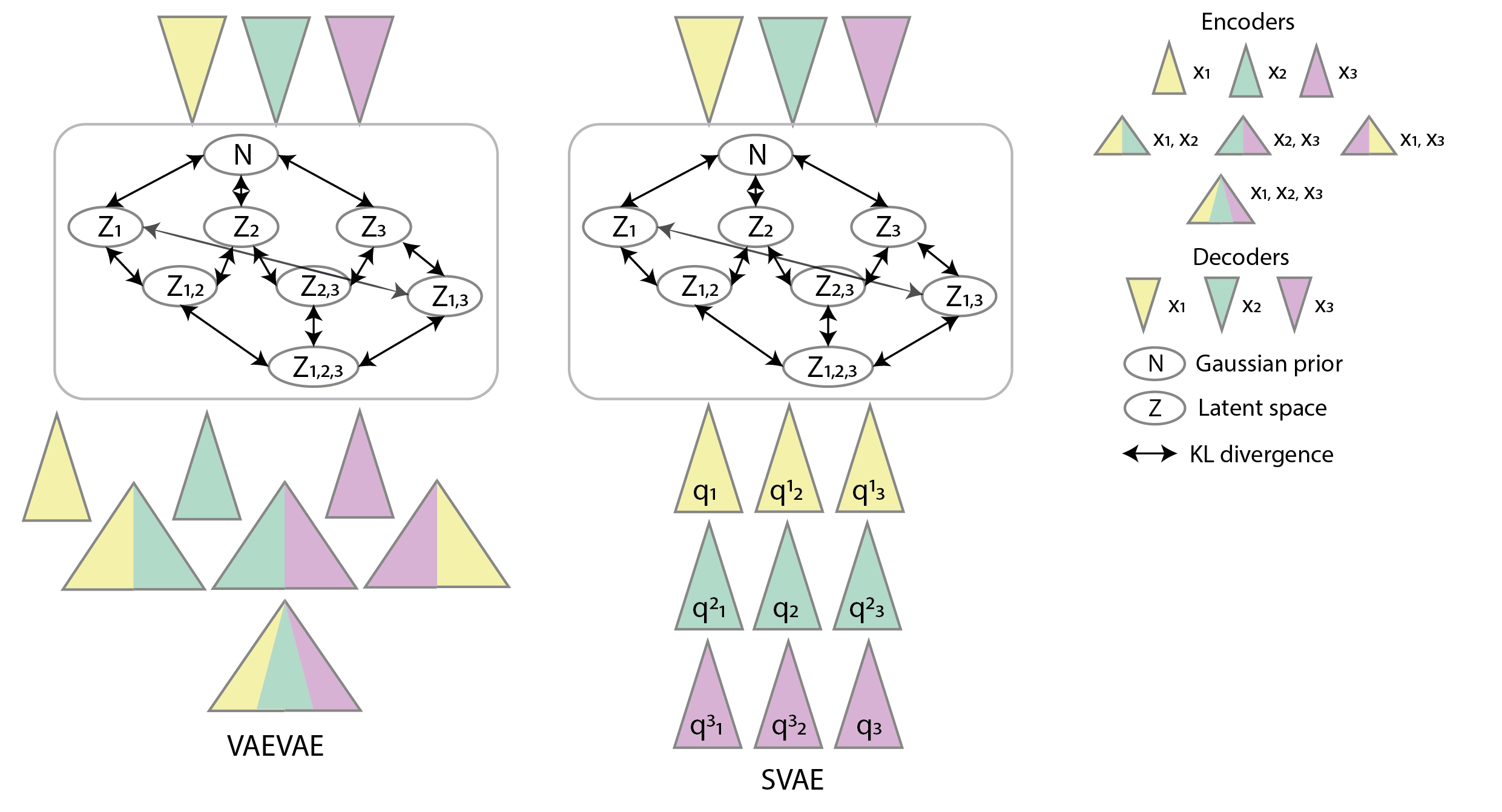
Figure 2: The SVAE and VAEVAE network architectures for 3-modalities. The number of parameters is $kn^{2}$ for SVAE and $kn2^{n-1}$ for VAEVAE, where $n$ is the number of modalities and $k$ is the number of parameters in one encoding network.

In the canonical extension of VAEVAE to three modalities, the three- and two-modal relations are captured by the corresponding networks $q(z|x_{1},x_{2},x_{3})$, $q(z|x_{i},x_{j})$ and $q(z|x_{i})$ for $i,j\in\{1,2,3\}$, see Figure 2. In the general $n$-modal case, the model has $2^{n}$ networks. For $n=3$, the loss function reads:

$$\mathcal{L}_{1,2,3}= E_{p_{\text{paired}}(x_{1},x_{2},x_{3})}\left[E_{q(z|x_{1},x_{2},x_{3})}[\log{p_{1}(x_{1}|z)}+\log{p_{2}(x_{2}|z)}+\log{p_{3}(x_{3}|z)}]\right]$$

$$-D_{\text{KL}}(q(z|x_{1},x_{2},x_{3})\;\|\;q(z|x_{1},x_{2}))$$

$$-D_{\text{KL}}(q(z|x_{1},x_{2},x_{3})\;\|\;q(z|x_{2},x_{3}))$$

$$-D_{\text{KL}}(q(z|x_{1},x_{2},x_{3})\;\|\;q(z|x_{1},x_{3}))$$ (29)

$$\mathcal{L}_{ij}= E_{p_{\text{paired}}(x_{1},x_{2},x_{3})}\left[E_{q(z|x_{i},x_{j})}[\log{p_{i}(x_{i}|z)}+\log{p_{j}(x_{j}|z)}]\right]$$

$$-D_{\text{KL}}(q(z|x_{i},x_{j})\;\|\;q(z|x_{1}))-D_{\text{KL}}(q(z|x_{i},x_{j})\;\|\;q(z|x_{2}))$$

$$-D_{\text{KL}}(q(z|x_{i},x_{j})\;\|\;q(z|x_{3}))-D_{\text{KL}}(q(z|x_{i},x_{j})\;\|\;q(z))$$ (30)

$$\mathcal{L}_{i}= E_{p_{\text{unpaired}}(x_{i})}\left[E_{q(z|x_{i})}[\log{p_{i}(x_{i}|z)}]-D_{\text{KL}}(q(z|x_{i})\;\|\;q(z))\right]$$ (31)

$$\mathcal{L}_{\text{comb}}= \mathcal{L}_{1,2,3}+\sum\limits_{i,j\in\{1,2,3\},i\neq j}\mathcal{L}_{i,j}+\sum\limits_{i=1}^{3}\mathcal{L}_{i}$$ (32)

In this study, we considered a simplifying extension of SVAE to $n$ modalities using $n^{2}$ networks $q_{i}^{j}(z|x_{j})$ for $i,j\in\{1,\dots,n\}$. For the 3-modal case depicted in Figure 2, the PoE relations between the modalities are defined in the following way:

$$q(z|x_{1},x_{2},x_{3}) =\frac{1}{Z(x_{1},x_{2},x_{3})}q_{1}^{1}(z|x_{1})q_{2}^{2}(z|x_{2})q_{3}^{3}(z|x_{3})$$ (33)

$$i,j,k\in\{1,2,3\},i\neq j\neq k:$$ (34)

$$q^{i}(z|x_{i},x_{j}) =\frac{i}{Z(x_{i},x_{j})}q_{i}^{i}(z|x_{i})q_{j}^{j}(z|x_{j})q_{k}^{i}(z|x_{i})$$ (35)

$$q^{j}(z|x_{i},x_{j}) =\frac{1}{Z(x_{i},x_{j})}q_{i}^{i}(z|x_{i})q_{j}^{j}(z|x_{j})q_{k}^{j}(z|x_{j})$$ (36)

$$q(z|x_{i}) =q_{i}^{i}(z|x_{i})q_{j}^{i}(z|x_{i})q_{k}^{i}(z|x_{i})$$ (37)

$$q(z) =\mathcal{N}(0,I)$$ (38)

The corresponding SVAE loss function has additional terms due to the fact that the relations between pairs of modalities need to be captured with two PoE rules $q^{i}(z|x_{i},x_{j})$ and $q^{i}(z|x_{i},x_{j})$ in SVAE, while there is only a single network $q(z|x_{i},x_{j})$ in VAEVAE. The loss functions equation 29–equation 32 above are modified in a way that $f(q(z|x_{i},x_{j}))=f(q^{i}(z|x_{i},x_{j}))+f(q^{j}(z|x_{i},x_{j}))$ for any function $f$.

This extension of the bi-modal case assumes that $p(x_{i},x_{j}|x_{k})=p(x_{i}|x_{k})p(x_{j}|x_{k})$ for $i,j,k\in\{1,2,3\},i\neq j\neq k$, which implies that $x_{i}$, $x_{j}$ and $x_{k}$ are independent of each other.

4 Experiments

We conducted experiments to compare state-of-the-art PoE based VAEs with the MoE approach MMVAE [8]. We considered VAEVAE (b) as proposed by [2] and SVAE as described above. The two approaches differ both in the underlying model as well as the objective function. For a better understanding of these differences, we also considered an algorithm referred to as VAEVAE*, which has the same model architecture as VAEVAE and the same loss function as SVAE. The difference in the training procedure for VAEVAE and VAEVAE* is shown in Algorithm 1. Since the VAEVAE implementation was not publicly available at the time of writing, we used our own implementation of VAEVAE based on the PiXYZ library. For details about the experiments we refer to Appendix A. The source code to reproduce the experiments can be found at https://github.com/sgalkina/poe-vaes. More qualitative examples are shown in Figure 3 for SVAE and VAEVAE.

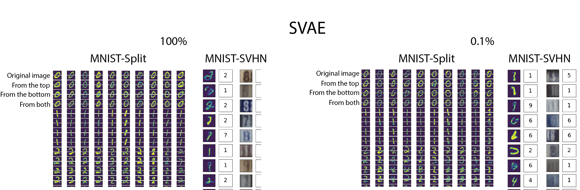
(a)

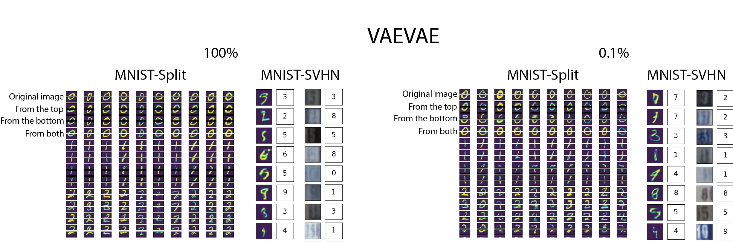
(b)

Figure 3: MNIST-Split image reconstructions of a top half and a bottom half given the top half, the bottom half of the original image or both halves. Side-by-side MNIST-SVHN reconstruction from randomly sampled latent space, with oracle predictions of a digit class. The joint coherence is a share of classes predicted the same. The examples are generated by SVAE and VAEVAE for the supervision levels 100% and 0.1%

For an unbiased evaluation, we considered the same test problems and performance metrics as [8]. In addition, we designed an experiment referred to as MNIST-Split that was supposed to be well-suited for PoE. In all experiments we kept the network architectures as similar as possible (see Appendix A). For the new benchmark problem, we constructed a multi-modal dataset where the modalities are similar in dimensionality as well as complexity and are providing missing information to each other rather than duplicating it. The latter should favor a PoE modelling, which suits an “AND” combination of the modalities.

We measured performance for different supervision levels for each dataset (e.g., 10% supervision level means that 10% of the training set samples were paired and the remaining 90% were unpaired).

Finally, we compared VAEVAE and SVAE on the real-world bioinformatics task that motivated our study, namely learning a joint representation of mass spectra and molecule structures.

4.1 Image and image: MNIST-Split

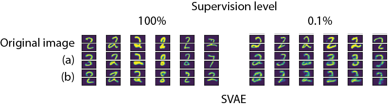
Figure 4: MNIST-Split image reconstructions of a top half and a bottom half given (a) the top half; (b) the bottom half of the original image.

We created an image reconstruction dataset based on MNIST digits [19]. The images were split horizontally into equal parts, either two or three depending on the experimental setting. These regions are considered as different input modalities.

Intuitively, for this task a joint representation should encode the latent class labels, the digits. The correct digit can sometimes be inferred from only one part of the image (i.e., one modality), but sometimes both modalities are needed. In the latter cases, an “AND” combination of the inputs is helpful. This is in contrast to the MNIST-SVHN task described below, where the joint label could in principle be inferred from each input modality independently.

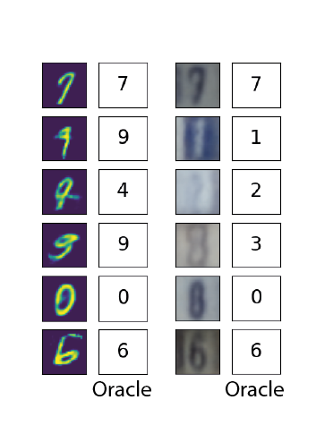
Figure 5: MNIST-SVHN reconstruction for fully supervised VAEVAE.

Two modalities: MNIST-Split.

In the bi-modal version referred to as MNIST-Split, the MNIST images were split in top and bottom halves of equal size, and the halves were then used as two modalities. We tested the quality of the image reconstruction given one or both modalities by predicting the reconstructed image label with an independent oracle network, a ResNet-18 [20] trained on the original MNIST dataset. The evaluation metrics were joint coherence, synergy, and cross-coherence. For measuring joint coherence, 1000 latent space vectors were generated from the prior and both halves of an image were then reconstructed with the corresponding decoding networks. The concatenated halves yield the fully reconstructed image. Since the ground truth class labels do not exist for the randomly sampled latent vectors, we could only perform a qualitative evaluation, see Figure 4. Synergy was defined as the accuracy of the image reconstruction given both halves. Cross-coherence considered the reconstruction of the full image from one half and was defined as the fraction of class labels correctly predicted by the oracle network.

Table 1: Evaluation of the models trained on the fully supervised datasets.

	Accuracy (both)	Accuracy (top half)	Accuracy (bottom half)
MMVAE	0.539	0.221	0.283
SVAE	0.948	0.872	0.816
VAEVAE	0.956	0.887	0.830
VAEVAE*	0.958	0.863	0.778

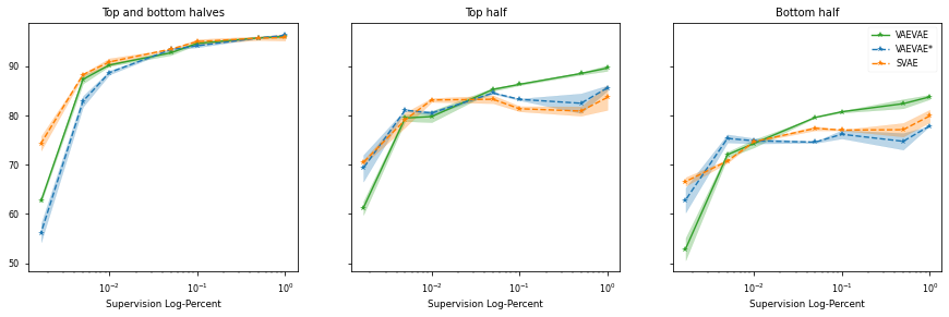
(a)

Figure 6: MNIST-Split dataset. Accuracy of an oracle network applied to images reconstructed given the full image (both halves), the top half and the bottom half.

The quantitative results are shown in Table 1 and Figure 6. All PoE architectures clearly outperformed MMVAE even when trained on the low supervision levels. In this experiment, it is important that both experts agree on a class label. Thus, as expected, the multiplicative PoE fits the task much better than the additive mixture. Utilizing the novel loss function (22) gave the best results for very low supervision (SVAE and VAEVAE*).

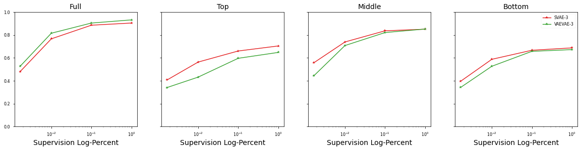
Figure 7: MNIST-Split-3 dataset, reproducing the logic of MNIST-Split for the input images split into three parts. The plots show the accuracy of an oracle network getting the full image or a single of the three single modalities (Top, Middle, Button) as inputs.

Three modalities: MNIST-Split-3.

We compared a simple generalization of the SVAE model to more than two modalities with the canonical extension of the VAEVAE model described in Section 3.5 on the MNIST-Split-3 data, the 3-modal version of MNIST-Split task. Figure 7 shows that SVAE performed better when looking at the reconstructions from individual modalities, but worse when all three modalities are given. While the number of parameters in the bi-modal case is the same for SVAE and VAEVAE, it grows exponentially for VAEVAE and stays in order of $n^{2}$ for SVAE where $n$ is the number of modalities, see Figure 2 and Section 3.5 for details.

4.2 Image and image: MNIST-SVHN

Figure 8: Performance on MNIST-SVHN for different supervision levels. (left) Joint coherence, a share of generated images with the same digit class; (middle) Cross-coherence, accuracy of SVHN reconstructions given MNIST; (right) Cross-coherence, accuracy of MNIST reconstructions given SVHN.

The first dataset considered by [8] is constructed by pairing MNIST and SVHN [21] images showing the same digit. This dataset shares some properties with MNIST-Split, but the relation between the two modalities is different: the digit class is derived from a concatenation of two modalities in MNIST-Split, while in MNIST-SVHN it could be derived from any modality alone. As before, oracle networks are trained to predict the digit classes of MNIST and SVHN images. Joint coherence was again computed based on 1000 latent space vectors generated from the prior. Both images were then reconstructed with the corresponding decoding networks. A reconstruction was considered correct if the predicted digit classes of MNIST and SVHN were the same. Cross-coherence was measured as above.

Figure 5 shows examples of paired image reconstructions from the randomly sampled latent space of the fully supervised VAEVAE model. The digit next to the each reconstruction shows the digit class prediction for this image. The quantitative results in Figure 8 show that all three PoE based models reached a similar joint coherence as MMVAE, VAEVAE scored even higher. The cross-coherence results were best for MMVAE, but the three PoE based models performed considerably better than the MVAE baseline reported by [8].

4.3 Image and text: CUB-Captions

The second benchmark considered by [8] is the CUB Images-Captions dataset [22] containing photos of birds and their textual descriptions. Here the modalities are of different nature but similar in dimensionality and information content. We used the source code by Shi et al. to compute the same evaluation metrics as in the MMVAE study. Canonical correlation analysis (CCA) was used for estimating joint and cross-coherences of images and text [23]. The projection matrices $W_{x}$ for images and $W_{y}$ for captions were pre-computed using the training set of CUB Images-Captions and are available as part of the source code. Given a new image-caption pair $\tilde{x},\tilde{y}$, we computed the correlation between the two by $\operatorname{corr}(\tilde{x},\tilde{y})=\frac{\phi(\tilde{x})^{T}\phi(\tilde{y})}{\left\lVert\phi(\tilde{x})\right\rVert\left\lVert\phi(\tilde{y})\right\rVert}$, where $\phi(\tilde{k})=W_{k}^{T}\tilde{k}-\operatorname{avg}(W_{k}^{T}k)$.

We employed the same image generation procedure as in the MMVAE study. Instead of creating the images directly, we generated 2048-d feature vectors using a pre-trained ResNet-101. In order to find the resulting image, a nearest neighbours lookup with Euclidean distance was performed. A CNN encoder and decoder was used for the (see Table A.5 and Table A.6). Prior to computing the correlations, the captions were converted to 300-d vectors using FastText [24]. As in the experiment before, we used the same network architectures and hyperparameters as [8]. We sampled 1000 latent space vectors from the prior distribution. Images and captions were then reconstructed with the decoding networks. The joint coherence was then computed as the CCA for the resulting image and caption averaged over the 1000 samples. Cross-coherence was computed from caption to image and vice versa using the CCA averaged over the whole test set.

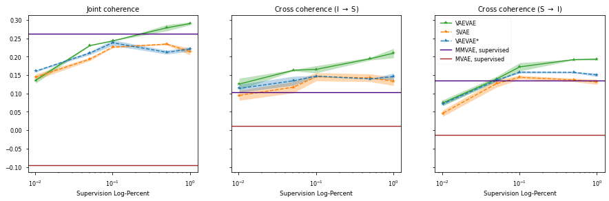
Figure 9: CUB Images-Captions dataset. Performance metrics for different supervision levels. (left) Joint coherence, the correlation between images and labels reconstructed from the randomly sampled latent vectors; (middle) Cross-coherence, the correlation of the reconstructed caption given the image; (right) Cross-coherence, the correlation of the reconstructed image given the caption.

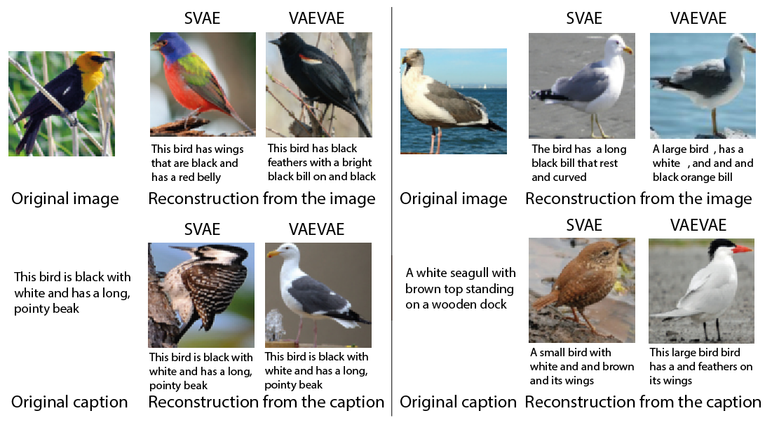
Figure 10: Examples of image and caption reconstructions given one modality input for SVAE and VAEVAE. Given that the caption can be broad (e.g., ”this bird is black and white and has a long pointy beak” in the example), it can fit many different images. In this case, the image from the caption reconstruction tends to better fit the description than the original image. The same goes for images: one of the reconstructed images has a bird with a red belly which got reflected in the generated caption even though it was not a part of the original caption.

As can be seen in Figure 9, VAEVAE showed the best performance among all models. With full supervision the VAEVAE model outperformed MMVAE in all three metrics. The cross-coherence of the three PoE models was higher or equal to MMVAE except for very low supervision levels. All three PoE based models were consistently better than MVAE.

4.4 Chemical structures and mass spectra

We evaluated SVAE and VAEVAE on a real-world bioinformatics application. The models were used for annotating mass spectra with molecule structures. Discovering chemical composition of a biological sample is one of the key problems in analytical chemistry. Mass spectrometry is a common high throughput analytical method. Thousands of spectra can be generated in a short time, but identification rates of the corresponding molecules is still low for most of the studies.

We approach the spectra annotation problem with bi-modal VAEs in the following way: the SVAE and VAEVAE models are trained on a subset of the MoNA (Mass Bank of North America) dataset [25], where the mass spectra suitable for molecule identification are assembled. We focused on tandem mass spectra from only one type of mass spectrometer collected in the positive ion mode. The mass spectra were the first modality. To represent a molecule structure, we used a molecule structural fingerprint, a bit string where an individual bit shows if a substructure from a predefined set of possible substructures is present in the molecule. Fingerprints of length $2149$ were used as the second modality. During testing, only the mass spectrum was provided and the fingerprint was predicted. A molecule structure still has to be identified based on the predicted structural fingerprint. We did this by ranking the candidate molecules from a molecule database based on the cross entropy loss between the molecule fingerprint and the predicted fingerprint.

For evaluation, we used competition data from the CASMI2017 (Critical Assessment of Small Molecule Identification) challenge [26]. Since the molecule structure identification is based on ranking the candidate list, we focused on the part of the challenge where the candidate list is already provided for each spectrum. In the preliminary experiments, SVAE outperformed VAEVAE in predicting molecule structural fingerprints from mass spectra, see Figure 11.

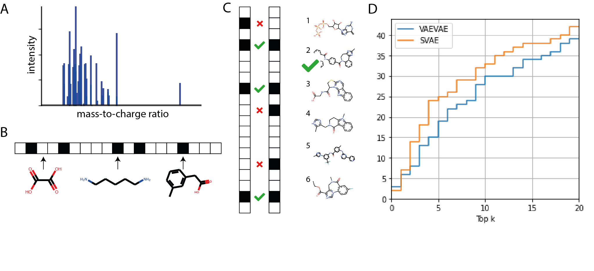
Figure 11: A) The first modality: a tandem mass spectrum; B) The second modality: a molecule structure fingerprint, a bit string where each bit represents if a given substructure is present in the molecule; C) The performance evaluation: the fingerprint is predicted with only the spectrum as input. The candidate molecules are ranked by cross-entropy loss between their fingerprints and the predicted fingerprint. The rank of the correct candidate is used for comparing the performance of different methods. D) The evaluation results for CASMI2017 challenge, with 112 test spectra and 200-10000 candidate molecules for each spectrum: The plot shows for how many spectra the correct candidate appeared in top $k$ candidates. SVAE performs better than VAEVAE in this preliminary evaluation.

5 Discussion and Conclusions

We studied bi-modal variational autoencoders (VAEs) based on a product-of-experts (PoE)architecture, in particular VAEVAE as proposed by [2] and a new model SVAE, which we derived in an axiomatic way, and represents a generalization of the VAEVAE architecture. The models learn representations that allow coherent sampling of the modalities and accurate sampling of one modality given the other. They work well in the semi-supervised setting, that is, not all modalities need to be always observed during training. It has been argued that the mixture-of-experts (MoE) approach MMVAE is preferable to a PoE for multimodal VAEs [8], in particular in the fully supervised setting (i.e., when all data are paired). This conjecture was based on a comparison with the MVAE model [7], but is refuted by our experiments showing that VAEVAE and our newly proposed SVAE can outperform MMVAE on experiments conducted by [8]. Intuitively, PoEs are more tailored to towards an “AND” (multiplicative) combination of the input modalities. This is supported by our experiments on halved digit images, where a conjunctive combination is helpful and the PoE models perform much better than MMVAE. In a real-world bioinformatics task, SVAE outperformed VAEVAE in predicting molecule structural fingerprints from mass spectra. We also expanded SVAE and VAEVAE to 3-modal case and show that SVAE demonstrates better performance on individual modalities reconstructions while having less parameters than VAEVAE.

Appendix A Details of experiments

The encoder and decoder architectures for each experiment and modality are listed below. To implement joint encoding network (VAEVAE architecture), an fully connected layer followed by ReLU is added to the encoding architecture for each modality. Another fully connected layer accepts the concatenated features from the two modalities as an input and outputs the latent space parameters. Adam optimiser is used for learning in all the models [27]. We used a padding of 1 pixel if the stride was 2 pixels and no padding otherwise.

MNIST-Split.

The models are trained for 200 epochs with the learning rate $2\cdot 10^{-4}$. The best epoch is chosen by the highest accuracy of the reconstruction from the top half evaluated on the validation set. We used a latent space dimensionality of $L=64$. The network architectures are described in Table A.2.

Encoder
Input $\in\mathbb{R}^{3\times 32\times 32}$
$4\times 4$ conv. 64 stride 2 ReLU
$4\times 4$ conv. 128 stride 2 ReLU
$4\times 4$ conv. 256 stride 2 ReLU
FC. 786 ReLU
FC. L, FC. L

Decoder
Input $\in\mathbb{R}^{L}$
FC. L ReLU
FC. 512 ReLU
FC. 112 ReLU
$4\times 4$ upconv. 56 stride 1 ReLU
$4\times 4$ upconv. 28 stride 2 ReLU

Table A.2: Network architectures for MNIST-Split for each image half.

MNIST-SVHN.

The models were trained for 50 epochs with learning rates $10^{-3}$ and $10^{-4}$. Only the results for the best learning rate are reported ($10^{-3}$ for VAEVAE and VAEVAE* and $10^{-4}$ for SVAE). The best epoch was chosen based on the highest joint coherence evaluated on the validation set. We used a latent space dimensionality of $L=20$. The network architectures are summarized in Table A.4 and Table A.3 for the MNIST and SVHN modality, respectively.

Encoder
Input $\in\mathbb{R}^{1\times 28\times 28}$
FC. 400 ReLU
FC. $L$, FC. $L$

Decoder
Input $\in\mathbb{R}^{L}$
FC. 400 ReLU
FC. 1 x 28 x 28 Sigmoid

Table A.3: Network architectures for MNIST-SVHN: MNIST.

Encoder
Input $\in\mathbb{R}^{3x32x32}$
$4\times 4$ conv. 32 stride 2 ReLU
$4\times 4$ conv. 64 stride 2 ReLU
$4\times 4$ conv. 128 stride 2 ReLU
$4\times 4$ conv. $L$ stride 1 , $4\times 4$ conv. $L$ stride 1

Decoder
Input $\in\mathbb{R}^{L}$
$4\times 4$ upconv. 128 stride 1 ReLU
$4\times 4$ upconv. 64 stride 2 ReLU
$4\times 4$ upconv. 32 stride 2 ReLU
$4\times 4$ upconv. 3 stride 2 Sigmoid

Table A.4: Network architectures for MNIST-SVHN: SVHN.

CUB-Captions.

The models were trained for 200 epochs with the learning rate $10^{-4}$. The best epoch was chosen based on the highest joint coherence evaluated on the validation set. We used a latent space dimensionality of $L=64$. The network architectures are described in Table A.5 and Table A.6 for the text and image modality, respectively.

Encoder
Input $\in\mathbb{R}^{1590}$
Word Emb. 256
$4\times 4$ conv. 32 stride 2 BatchNorm2d ReLU
$4\times 4$ conv. 64 stride 2 BatchNorm2d ReLU
$4\times 4$ conv. 128 stride 2 BatchNorm2d ReLU
$1\times 4$ conv. 256 stride $1\times 2$ pad $0\times 1$ & BatchNorm2d ReLU
$1\times 4$ conv. 512 stride $1\times 2$ pad $0\times 1$ & BatchNorm2d ReLU
$4\times 4$ conv. $L$ stride 1 , $4\times 4$ conv. $L$ stride 1

Decoder
Input $\in\mathbb{R}^{L}$
$4\times 4$ upconv. 512 stride 1 ReLU
$1\times 4$ upconv. 256 stride $1\times 2$ pad $0\times 1$ & BatchNorm2d ReLU
$1\times 4$ upconv. 128 stride $1\times 2$ pad $0\times 1$ & BatchNorm2d ReLU
$4\times 4$ upconv. 64 stride 2 BatchNorm2d ReLU
$4\times 4$ upconv. 32 stride 2 BatchNorm2d ReLU
$4\times 4$ upconv. 1 stride 2 ReLU
Word Emb.${}^{\text{T}}$ 1590

Table A.5: Network architectures for CUB-Captions language processing.

Encoder
Input $\in\mathbb{R}^{2048}$
FC. 1024 ELU
FC. 512 ELU
FC. 256 ELU
FC. L, FC. L

Decoder
Input $\in\mathbb{R}^{L}$
FC. 256 ELU
FC. 512 ELU
FC. 1024 ELU
FC. 2048

Table A.6: Network architectures for CUB-Captions image processing.

MNIST-Split-Three.

The models were trained for 50 epochs with the learning rate $2\cdot 10^{-4}$. The best epoch was chosen by the highest accuracy of the reconstruction from the top half evaluated on the validation set. We used a latent space dimensionality of $L=64$. The network architectures are described in Table A.7.

Encoder
Input $\in\mathbb{R}^{3x32x32}$
$4\times 4$ conv. 64 stride 2 ReLU
$4\times 4$ conv. 128 stride 2 ReLU
$4\times 4$ conv. 256 stride 2 ReLU
FC. 786 ReLU
FC. L, FC. L

Decoder
Input $\in\mathbb{R}^{L}$
FC. L ReLU
FC. 512 ReLU
FC. 112 ReLU
$4\times 4$ upconv. 56 stride 1 ReLU
$2\times 4$ upconv. 28 stride 2 ReLU

Table A.7: Network architectures for MNIST-Split-Three for each image part.

Spectra and molecule fingerprints.

The models were trained for 140 epochs with the learning rate $10^{-4}$. The best epoch was chosen by the highest accuracy of the test set. We used a latent space dimensionality of $L=300$. The network architectures are described in Table A.8 and Table A.9.

Encoder
Input $\in\mathbb{R}^{11000}$
FC. 10000 & BatchNorm1d ReLU
FC. 5000 & BatchNorm1d ReLU
FC. 2048 & BatchNorm1d ReLU
FC. L, FC. L

Decoder
Input $\in\mathbb{R}^{L}$
FC. 3000 & BatchNorm1d ReLU
FC. 5000 & BatchNorm1d ReLU
FC. 10000 & BatchNorm1d ReLU
FC. 11000

Table A.8: Network architectures for the spectra-fingerprints experiment, spectra modality.

Encoder
Input $\in\mathbb{R}^{2149}$
FC. 1024 ReLU
FC. 1000 ReLU
FC. L, FC. L

Decoder
Input $\in\mathbb{R}^{L}$
FC. 500 ReLU
FC. 1024 ReLU
FC. 2149 & Sigmoid

Table A.9: Network architectures for the spectra-fingerprints experiment, fingerprints modality.

References

- [1] O. Caglayan, P. Madhyastha, L. Specia, L. Barrault, Probing the need for visual context in multimodal machine translation, in: Proceedings of the 2019 Conference of the North American Chapter of the Association for Computational Linguistics: Human Language Technologies (NAACL HLT), Vol. 1, 2019, pp. 4159–4170.
- [2] M. Wu, N. Goodman, Multimodal generative models for compositional representation learning, arXiv:1912.05075 (2019).
- [3] J. E. van Engelen, H. H. Hoos, A survey on semi-supervised learning, Machine Learning 109 (2) (2020) 373–440.
- [4] D. P. Kingma, M. Welling, Auto-encoding variational Bayes, in: International Conference on Learning Representations (ICLR), 2014.
- [5] G. E. Hinton, Training products of experts by minimizing contrastive divergence, Neural Computation 14 (8) (2002) 1771–1800.
- [6] M. Welling, Product of experts, Scholarpedia 2 (10) (2007) 3879.
- [7] M. Wu, N. Goodman, Multimodal generative models for scalable weakly-supervised learning, in: Advances in Neural Information Processing Systems 31 (NIPS), 2018, pp. 5575–5585.
- [8] Y. Shi, S. N, B. Paige, P. Torr, Variational mixture-of-experts autoencoders for multi-modal deep generative models, in: Advances in Neural Information Processing Systems (NeurIPS), 2019, pp. 15718–15729.
- [9] W. Wang, X. Yan, H. Lee, K. Livescu, Deep variational canonical correlation analysis, arXiv:1610.03454 (2016).
- [10] K. Sohn, H. Lee, X. Yan, Learning structured output representation using deep conditional generative models, in: Advances in Neural Information Processing Systems (NeurIPS), 2015, pp. 3483–3491.
- [11] Y. Tian, J. Engel, Latent translation: Crossing modalities by bridging generative models, arXiv:1902.08261 (2019).
- [12] C. Silberer, M. Lapata, Learning grounded meaning representations with autoencoders, in: Proceedings of the 52nd Annual Meeting of the Association for Computational Linguistics (ACL), Vol. 1, Association for Computational Linguistics, 2014, pp. 721–732.
- [13] J. Ngiam, A. Khosla, M. Kim, J. Nam, H. Lee, A. Y. Ng, Multimodal deep learning, in: Proceedings of the 28th International Conference on International Conference on Machine Learning (ICML), 2011, p. 689–696.
- [14] D. P. Kingma, S. Mohamed, D. J. Rezende, M. Welling, Semi-supervised learning with deep generative models, in: Advances in Neural Information Processing Systems (NeurIPS), 2014, pp. 3581–3589.
- [15] M. Suzuki, K. Nakayama, Y. Matsuo, Joint Multimodal Learning with Deep Generative Models, in: International Conference on Learning Representations Workshop (ICLR) Workshop Track, 2017.
- [16] D. J. Rezende, S. Mohamed, D. Wierstra, Stochastic backpropagation and approximate inference in deep generative models, in: Proceedings of the 31st International Conference on Machine Learning (ICML), Vol. 32(2) of Proceedings of Machine Learning Research, PMLR, 2014, pp. 1278–1286.
- [17] R. N. Yadav, A. Sardana, V. P. Namboodiri, R. M. Hegde, Bridged variational autoencoders for joint modeling of images and attributes, 2020 IEEE Winter Conference on Applications of Computer Vision (WACV) (2020) 1468–1476.
- [18] Y. Burda, R. Grosse, R. Salakhutdinov, Importance weighted autoencoders, in: International Conference on Learning Representations (ICLR), 2016. arXiv:1509.00519.
- [19] Y. LeCun, L. Bottou, Y. Bengio, P. Haffner, Gradient-based learning applied to document recognition, Proceedings of the IEEE 86 (11) (1998) 2278–2324.
- [20] K. He, X. Zhang, S. Ren, J. Sun, Deep residual learning for image recognition, in: 2016 IEEE Conference on Computer Vision and Pattern Recognition (CVPR), 2016, pp. 770–778.
- [21] Y. Netzer, T. Wang, A. Coates, A. Bissacco, B. Wu, A. Y. Ng, Reading digits in natural images with unsupervised feature learning, in: NIPS Workshop on Deep Learning and Unsupervised Feature Learning 2011, 2011.
- [22] C. Wah, S. Branson, P. Welinder, P. Perona, S. Belongie, The Caltech-UCSD Birds-200-2011 Dataset, Tech. Rep. CNS-TR-2011-001, California Institute of Technology (2011).
- [23] D. Massiceti, P. K. Dokania, N. Siddharth, P. H. S. Torr, Visual dialogue without vision or dialogue, in: NeurIPS Workshop on Critiquing and Correcting Trends in Machine Learning, 2018. arXiv:1812.06417.
- [24] P. Bojanowski, E. Grave, A. Joulin, T. Mikolov, Enriching word vectors with subword information, Transactions of the Association for Computational Linguistics 5 (2017) 135–146.
-
[25]
M. Vinaixa, E. L. Schymanski, S. Neumann, M. Navarro, R. M. Salek, O. Yanes,
Mass
spectral databases for LC/MS- and GC/MS-based metabolomics: State of the
field and future prospects, TrAC Trends in Analytical Chemistry 78 (2016)
23–35.
doi:10.1016/J.TRAC.2015.09.005.
URL https://www.sciencedirect.com/science/article/pii/S0165993615300832 -
[26]
E. L. Schymanski, C. Ruttkies, M. Krauss, C. Brouard, T. Kind, K. Dührkop,
F. Allen, A. Vaniya, D. Verdegem, S. Böcker, J. Rousu, H. Shen,
H. Tsugawa, T. Sajed, O. Fiehn, B. Ghesquière, S. Neumann,
Critical assessment of small
molecule identification 2016: automated methods, Journal of Cheminformatics
9 (1) (Mar. 2017).
doi:10.1186/s13321-017-0207-1.
URL https://doi.org/10.1186/s13321-017-0207-1 - [27] D. P. Kingma, J. Ba, Adam: A method for stochastic optimization, in: International Conference on Learning Representations (ICLR), 2015.