Enhancing Population Persistence by a Protection Zone in a Reaction-Diffusion Model with Strong Allee Effect

Abstract

Protecting endangered species has been an important issue in ecology. We derive a reaction-diffusion model for a population in a one-dimensional bounded habitat, where the population is subjected to a strong Allee effect in its natural domain but obeys a logistic growth in a protection zone. We establish the conditions for population persistence and extinction via the principal eigenvalue of an associated eigenvalue problem and investigate the dependence of this principal eigenvalue on the location (i.e., the starting point and the length) of the protection zone. The results are used to design the optimal protection zone under different boundary conditions, that is, to suggest the starting point and length of the protection zone with respect to different population growth rate in the protection zone, in order for the population to persist in a long term.

Key words. A reaction-diffusion model; strong Allee effect; protection zone; population persistence; principal eigenvalue.

MSC2020: 34B09; 35B40; 35K55; 92D25.

1 Introduction and our model

1.1 Introduction

Endangered species or native species may be subjected to density decline due to various reasons such as climate change, habitat change, pollution, predation, harvest, invasion of alien species, etc. Strategies or management plans have been designed in order to maintain the species and their habitats at a certain level so that the populations can continue to grow and influence the habitats and the associated ecosystems in a healthy manner. Establishing protection zones such as natural reserves has been considered as an effective method to protect endangered species from extinction, or otherwise to slow down the speed of its extinction; see e.g., [28, 29, 3, 31, 36, 25].

The Allee effect is a ubiquitous phenomenon in biology showing that the population growth rate can be significantly small or even negative when the population density or size is very low, due to e.g., the difficulty in finding mates or defending against predators, and that the population growth rate is also negative when the population density or size exceeds a large number due to the environment limit; see e.g., [1, 10, 23]. In particular, it is referred to a strong Allee effect if the growth rate is negatively related to the population size or a weak Allee effect if the growth rate is positively related to the population size, when the population size is small. This phenomenon has been observed, for instance, for the west Atlantic cod (Ganus morhus) (see e.g., [13]), Vancouver Island marmot (Marmota vancouverensis) (see e.g., [5]), and marine species such as blue crab, oyster (see e.g., [23]). The Allee effect has been increasingly studied in population models in recent decades. The dynamics of a single species with Allee effect has been explored in e.g., [45, 44, 15, 52, 34, 53, 54, 42]; the dynamics of predator-prey models with Allee effect on the prey has been investigated in e.g., [11, 37, 48, 49].

When a species is subjected to significant predation, harvest, or competition, establishing protection zones, where its population can enter or exit freely but its predators, competitors, or human beings are prohibited from entering, allows the species to freely grow and be preserved within the protection zones. Population models have been developed to predict and evaluate population responses to management actions such as protection zones that affect growth, survival, and spread. Reaction-diffusion predator-prey models and competition models with protection zones for the prey or for the weak competitor were first investigated in a sequence of works by Du et al, in [19] for a Holling type II predator-prey system, in [16, 22] for the competition system, in [18] for a Leslie type predator-prey system, and in [20] for predator-prey systems with protection coefficients. Results there showed that the prey or the weak competitor can successfully survive with the other species if the size of the protection zone is large enough while situations may be complicated and the persistence of the species may depend on demographic and dispersal characteristics of all involved species as well as the habitat features if the size of the protection zone is small. The effect of cross-diffusion on the stationary problem (i.e., the problem for the steady state) was studied for predator-prey systems with protection zones in [38, 35] and for a Lotka-Voltera competition system with a protection zone in [51]. Predator-prey systems with protection zones for the prey were also studied in [26, 46] (with Beddington-DeAngelis type functional response), in [9] (with a prey refuge where a constant amount of preys are protected from being predated), and in [11] (with a protection zone and strong Allee effect for the prey). For a single species living in a habitat where a protection zone is set up in a natural domain where the population is subjected to extra removal due to external reasons, its dynamics was studied in e.g., [21, 55] (in a temporally constant environment), in [14] (in random environments), and in [12] (with spatially heterogeneous harvesting quota). In particular, when a single species was subjected to strong Allee effect outside of the protection zones, reaction-diffusion models were applied to investigate the role of the length and the structure (one single connected patch or separated patches) of the protection zones on species spreading in [15], as well as the effect of protection zones on the long-term behaviors and spread of a species with free boundary conditions in [45, 44].

In this work, we are interested in the effect of the protection zone on the long-term dynamics of an endangered species with spatial dispersal and how the protection zone can enhance population persistence of the species. Our main purpose is to suggest strategies for the placement of an optimal protection zone in order for the population to persist when the initial population density is small. Note that it may be very difficult for an endangered species to recover when its density is sufficiently low. We assume that the population is subjected to a strong Allee effect in its natural domain so that such a species will die out if its initial population size is small. To help the population persist, a protection zone is set up in its domain and in this zone the population can keep growing to its carrying capacity. We will study a reaction-diffusion system that describes the dynamics of the population in such a habitat. Previous studies have discovered that a large size of the protection zone can usually help population persist (see e.g., [19, 16, 18, 21, 55]). We will establish population persistence and extinction via the principal eigenvalue of the eigenvalue problem associated with the linearized system at the trivial solution. Then we will derive the precise influence of the protection zone, specifically, the starting point and the length of the protection zone, on the persistence conditions under different boundary conditions via the investigation of the dependence of the principal eigenvalue on these factors. Based on these results, we will then design the optimal location of the protection zone in each case.

1.2 Our model

To describe the spatiotemporal evolution of a single species that is subjected to the strong Allee effect growth, we consider a reaction-diffusion equation on a one-dimensional bounded habitat $(0,L)$:

$$u_{t}=u_{xx}+g(u),\quad 0<x<L,\;\;t>0,$$ (1.1)

where $u(t,x)$ is the density of the population at location $x$ at time $t$, $L$ is the total length of the habitat represented by the interval $[0,L]$. The growth rate $g(u)$ satisfies the following basic technical assumptions, which are similar to those in [7, 42]:

1. $g\in C^{1}([0,+\infty))$, $g^{\prime}(0)<0=g(0)=g(a)=g(1)$ with $0<a<1$, $g(u)$ is positive for $a<u<1$, and $g(u)$ is negative otherwise.

Here the local carrying capacity of $g$ is rescaled as $1$, and $a$ is the local threshold value for the extinction/persistence of the population, which is also known as the sparsity constant. The most important feature of (1.1) is that it admits bistable steady states, and different initial conditions can lead to different asymptotic behaviors of the solutions [54]. Especially, $\lim\limits_{t\rightarrow\infty}u(t,x)=0$ provided that the initial quantity is below $a$. Hence, the persistence is always conditional.

Another universal acceptable growth for a single species is the logistic type, which leads to the following problem:

$$u_{t}=u_{xx}+f(u),\quad 0<x<L,\;\;t>0,$$ (1.2)

where the growth rate $f(u)$ satisfies the following basic technical assumptions, which are similar to those in [42]:

1. $f\in C^{1}([0,+\infty))$, $f^{\prime}(0)>0=f(0)=f(1)$, $f(u)$ is positive for $0<u<1$, and $f(u)$ is negative otherwise.

For simplicity, the local carrying capacity of $f$ is also rescaled as $1$. It is well known that all solutions of problem (1.2) with non-negative and not identically zero initial data will converge to the steady state $u=1$ as $t\rightarrow+\infty$. It leads to an unconditional persistence of the population for all initial condition.

Typical examples of strong Allee effect growth functions and logistic growth functions are

$$g(u)=ru(1-u)(u-a),\quad f(u)=ru(1-u),$$ (1.3)

where $r>0$ represents the intrinsic growth rate of the population, and $a\in(0,1)$ indicates that the population growth rate becomes negative when its density is below $a$.

To conserve an endangered species in a bounded region, one effective way is to introduce a protection zone within which the population’s continuous growth is guaranteed. Mathematically, one may use the strong Allee effect growth to describe the dynamics of the endangered species in its natural domain, and a logistic type growth for its dynamics in the protection zone. As a result, we are led to consider the following model that describes the dynamics of a population in a one-dimensional habitat with a protection zone:

$$\begin{cases}u_{t}=u_{xx}+F(u),&\,x\in(0,L),\ \ t>0,\\ u(0,x)=u_{0}(x)\geq 0,&\,x\in(0,L),\end{cases}$$ (1.4)

where

$$F(u)=\left\{\begin{array}[]{l}f(u),\quad x\in(\alpha,\alpha+l),\\ g(u),\quad x\in(0,\alpha)\cup(\alpha+l,L).\end{array}\right.$$

Here, $(\alpha,\alpha+l)$ represents a protection zone with starting point $\alpha$ and length $l>0$ satisfying $0\leq\alpha<\alpha+l\leq L$. Note that the species follows the strong Allee effect growth $g(u)$ on $(0,\alpha)\cup(\alpha+l,L)$, while it obeys the logistic growth $f(u)$ in the protection zone $(\alpha,\alpha+l)$, and that $g$ and $f$ satisfy the conditions in (A1) and (A2), respectively. We will use general functions $g$ and $f$ to derive our theories, but use specific examples of $g$ and $f$ in (1.3) in numerical simulations.

Boundary conditions at $x=0$ and $x=L$ can be assumed to be a general Robin type:

$$\alpha_{1}u_{x}(t,0)-\alpha_{2}u(t,0)=0,\quad\alpha_{1}\geq 0,\quad\alpha_{2}\geq 0,\quad\alpha_{1}^{2}+\alpha_{2}^{2}\neq 0,\quad t>0,$$ (1.5a)

$$\beta_{1}u_{x}(t,L)+\beta_{2}u(t,L)=0,\quad\beta_{1}\geq 0,\quad\beta_{2}\geq 0,\quad\beta_{1}^{2}+\beta_{2}^{2}\neq 0,\quad t>0,$$ (1.5b)

which typically includes special boundary conditions such as

$$\begin{array}[]{lllll}\text{Neumann condition: }&u_{x}(t,0)=0&\text{ or }&u_{x}(t,L)=0,&t>0,\\ \text{Dirichlet condition: }&u(t,0)=0&\text{ or }&u(t,L)=0,&t>0.\end{array}$$ (1.6)

For any given $u_{0}\in C([0,L])$, it is easy to check that equation (1.4)-(1.5) admits a unique solution $u(\cdot,\cdot)\in C^{1,2}((0,\infty)\times([0,L]\backslash\{\alpha,\alpha+l\}))\cap C^{\frac{\gamma}{2},1+\gamma}((0,\infty)\times[0,L])\cap C([0,\infty)\times[0,L])$ for any $\gamma\in(0,1)$ and $u(t,\cdot)$ exists for all $t>0$, and that if $u_{0}\geq 0,\not\equiv 0$, then $u(t,x)>0$ for all $(t,x)\in(0,\infty)\times[0,L]$ except at the Dirichlet boundary ends; see e.g., [33, 4]. Moreover, a simple comparison analysis gives $\limsup\limits_{t\rightarrow\infty}u(t,x)\leq 1$ for any nonnegative solution.

Given $t>0$, since any nonnegative solution $u(t,x)$ of (1.4)-(1.5) is continuously differentiable at the interface points $\alpha$ and $\alpha+l$, this means biologically that the population density is continuous and the population flux is conserved at these points, where the population growth conditions change.

The rest of the paper is organized as follows. In section 2, we will present general theories for population persistence and extinction by virtue of the principal eigenvalue of the associated eigenvalue problem for the linearized equation at the trivial solution. In section 3, we will study the dependence of the principal eigenvalue on the starting point and the length of the protection zone under different sets of boundary conditions and then provide management plans for setting up the protection zone. Section 4 ends the paper with a brief discussion of the biological implications of the obtained results and some perspective of future work. In the appendix, we present the detailed calculation of Lemmas 3.5 and 3.6.

2 The theories for population persistence and extinction

In this section, we will establish theories for population persistence and extinction for (1.4)-(1.5). We first introduce some function spaces. In the case of Neumann or Robin boundary conditions, let $\mathbb{X}=C^{1}([0,L],\mathbb{R})$ denote the Banach space of continuously differentiable functions on $[0,L]$ with the norm $\textstyle\|u\|=\max\limits_{x\in[0,L]}|u(x)|+\max\limits_{x\in[0,L]}|u^{\prime}(x)|$ for $u\in\mathbb{X}$. The set of nonnegative functions forms a solid cone $\mathbb{X}_{+}$ in $\mathbb{X}$ with interior $Int(\mathbb{X}_{+})=\{u\in\mathbb{X}:u(x)>0,\forall x\in[0,L]\}$. In the case of Dirichlet boundary conditions, let $\mathbb{X}=C_{0}([0,L],\mathbb{R})\cap C^{1}([0,L],\mathbb{R})$ be the set of continuously differentiable functions on $[0,L]$ vanishing on the boundary with the norm $\textstyle||u||=\max\limits_{x\in[0,L]}|u(x)|+\max\limits_{x\in[0,L]}|u^{\prime}(x)|$. The set of nonnegative functions $\mathbb{X}_{+}$ forms a solid cone in $X$ with nonempty interior in $X$ given by $Int(\mathbb{X}_{+})=\{u\in\mathbb{X}_{+}:u(x)>0\mbox{ for all }x\in(0,L),u_{x}(0)>0,u_{x}(L)<0\}$. If one of the boundary conditions is Neumann or Robin and the other one is Dirichlet, the function space $\mathbb{X}$ can be similarly defined.

The linearized problem of (1.4)-(1.5) at $u=0$ satisfies

$$\left\{\begin{array}[]{l}\displaystyle u_{t}=u_{xx}-H(x)u,\quad x\in(0,L),\quad t>0,\\ \text{ with boundary conditions as in (\ref{udbcs})},\end{array}\right.$$ (2.1)

where

$$H(x)=\begin{cases}-f^{\prime}(0),&x\in(\alpha,\alpha+l),\\ -g^{\prime}(0),&x\in(0,\alpha)\cup(\alpha+l,L).\end{cases}$$ (2.2)

Letting $u(t,x)=e^{-\lambda t}\varphi(x)$, we obtain the eigenvalue problem associated with (2.1):

$$\left\{\begin{array}[]{ll}-\varphi_{xx}+H(x)\varphi=\lambda\varphi,&\quad x\in(0,L),\\ \alpha_{1}\varphi^{\prime}(0)-\alpha_{2}\varphi(0)=0,&\quad\beta_{1}\varphi^{\prime}(L)+\beta_{2}\varphi(L)=0.\end{array}\right.$$ (2.3)

It is well-known that (2.3) admits a unique principal eigenvalue, denoted by $\lambda_{1}(\alpha,l)$, associated with a positive eigenfunction in $Int(X_{+})$, denoted by $\varphi_{1}$. Indeed, it follows from standard elliptic regularity theory that $\varphi_{1}\in C^{2}([0,L]\backslash\{\alpha,\,\alpha+l\})\cap C^{1}([0,L])$.

We now use the principal eigenvalue $\lambda_{1}(\alpha,l)$ of (2.3) to establish population persistence or extinction for (1.4)-(1.5). The main result in this section is given as below.

Theorem 2.1.

The following statements hold.

1. If $\lambda_{1}(\alpha,l)<0$, then the population will be uniformly persistent in the sense that there exists $\xi_{0}>0$ such that for any $\phi\in\mathbb{X}_{+}\setminus\{\mathbf{0}\}$, the solution $u(t,x)$ of (1.4)-(1.5) with the initial data $\phi$ satisfies

   $$\liminf_{t\rightarrow\infty}u(t,x)\geq\xi_{0},\ \mbox{ uniformly for }x\in[0,L],$$ (2.4)

   in the case of Robin boundary conditions or

   $$\liminf_{t\rightarrow\infty}u(t,x)\geq\xi_{0}\tilde{e}(x),\ \mbox{ uniformly for }x\in[0,L],$$ (2.5)

   in the case of Dirichlet boundary conditions, where $\tilde{e}(\cdot)$ is a given positive element in $Int(\mathbb{X}_{+})$.

2. If $\lambda_{1}(\alpha,l)>0$, then there exist small initial data in $\mathbb{X}_{+}$ such that $\limsup\limits_{t\rightarrow\infty}u(t,x)=0$ uniformly for $x\in[0,L]$.

Proof.

(i). Note that the problem (1.4)-(1.5) has a unique solution in $\mathbb{X}$ and the solution to (1.4)-(1.5) remains nonnegative on its interval of existence if it is nonnegative initially (see e.g., [33, 4]). Let $\{\Phi_{t}\}_{t\geq 0}$ be the semiflow generated by (1.4)-(1.5) such that $u(t,x)=\Phi_{t}(u_{0})(x)$, where $u(t,x)$ is the solution of (1.4)-(1.5) with initial condition $u_{0}$. Then $\Phi_{t}:\mathbb{X}_{+}\rightarrow\mathbb{X}_{+}$ is point dissipative since for any initially nonnegative continuous data $u_{0}$, the solution $u(t,x)$ satisfies $0\leq\limsup\limits_{t\rightarrow\infty}u(t,x)\leq 1$ for all $x\in[0,L]$. Moreover, the maximum principle also implies that for any $v\in\mathbb{X}_{+}\setminus\{\mathbf{0}\}$, $\Phi_{t}(v)(x)>0$ for all $t>0$ and $x\in[0,L]$ except at the Dirichlet boundary point(s). Obviously, $\Phi_{t}:\mathbb{X}_{+}\rightarrow\mathbb{X}_{+}$ is compact for all $t>0.$ By [24, Theorem 3.4.8], it follows that $\Phi_{t}:\mathbb{X}_{+}\rightarrow\mathbb{X}_{+}$ ($t>0$), has a global compact attractor.

We now state the following claim: there exists $\delta_{0}>0$ such that

$$\limsup\limits_{t\rightarrow\infty}||\Phi_{t}(v)||\geq\delta_{0},\ \forall v\in\mathbb{X}_{+}\setminus\{\mathbf{0}\}.$$

To this end, let $\varphi_{1}\in\mathbb{X}_{+}$ be a positive eigenfunction of the eigenvalue problem (2.3) corresponding to the principal eigenvalue $\lambda_{1}(\alpha,l)<0$. Then there exists a sufficiently small $\epsilon_{0}>0$ such that for any $\epsilon\in(0,\epsilon_{0})$, the eigenvalue problem

$$\left\{\begin{array}[]{ll}\displaystyle-\varphi_{xx}-(f^{\prime}(0)-\epsilon)\varphi=\lambda\varphi,&\quad x\in(\alpha,\alpha+l),\\ \displaystyle-\varphi_{xx}-(g^{\prime}(0)-\epsilon)\varphi=\lambda\varphi,&\quad x\in(0,\alpha)\cup(\alpha+l,L),\\ \alpha_{1}\varphi^{\prime}(0)-\alpha_{2}\varphi(0)=0,&\quad\beta_{1}\varphi^{\prime}(L)+\beta_{2}\varphi(L)=0\end{array}\right.$$ (2.6)

admits a principal eigenvalue $\lambda_{1}^{\epsilon}<0$ with a positive eigenfunction $\varphi_{1}^{\epsilon}\in\mathbb{X}_{+}$. Let $\bar{\epsilon}\in(0,\epsilon_{0})$. By the continuity of $f$ and $g$, there exists a $\delta_{0}>0$ such that $f(u)>(f^{\prime}(0)-\bar{\epsilon})u$ and $g(u)>(g^{\prime}(0)-\bar{\epsilon})u$ when $0<u<\delta_{0}$ for all $x\in[0,L]$. Assume, for the sake of contradiction, that there exists $v_{0}\in\mathbb{X}_{+}\setminus\{\mathbf{0}\}$ such that the solution $u(t,x)=\Phi_{t}(v_{0})(x)$ of (1.4)-(1.5) with the initial value $v_{0}$ satisfies

$$\limsup\limits_{t\rightarrow\infty}||\Phi_{t}(v_{0})||<\delta_{0}.$$ (2.7)

Then there exists a large $t_{0}>0$, such that $u(t,x)<\delta_{0}$ for all $x\in[0,L]$ and $t\geq t_{0}$, and hence, $f(u)>(f^{\prime}(0)-\bar{\epsilon})u$ and $g(u)>(g^{\prime}(0)-\bar{\epsilon})u$ for all $x\in[0,L]$ and $t\geq t_{0}.$ Therefore, it holds that

$$\left\{\begin{array}[]{ll}\displaystyle u_{t}=u_{xx}+f(u)>u_{xx}+(f^{\prime}(0)-\bar{\epsilon})u,&\,x\in(\alpha,\alpha+l),\\ \displaystyle u_{t}=u_{xx}+g(u)>u_{xx}+(g^{\prime}(0)-\bar{\epsilon})u,&\,x\in(0,\alpha)\cup(\alpha+l,L),\end{array}\right.$$ (2.8)

for all $t\geq t_{0}$. Since $u(t_{0},\cdot)\in\mbox{Int }\mathbb{X}_{+}$, we can choose a sufficiently small number $\eta>0$, such that $u(t_{0},\cdot)\geq\eta\varphi_{1}^{\bar{\epsilon}}(\cdot)$, where $\varphi_{1}^{\bar{\epsilon}}$ is the positive eigenfunction of (2.6) (with $\epsilon=\bar{\epsilon}$) corresponding to $\lambda_{1}^{\bar{\epsilon}}$. Note that for $t\geq t_{0}$, $\eta e^{-\lambda_{1}^{\bar{\epsilon}}(t-t_{0})}\varphi_{1}^{\bar{\epsilon}}(x)$ is the unique solution of

$$\left\{\begin{array}[]{l}\displaystyle\bar{u}_{t}=\bar{u}_{xx}+(f^{\prime}(0)-\bar{\epsilon})\bar{u},\quad x\in(\alpha,\alpha+l),\ \ t>t_{0},\\ \displaystyle\bar{u}_{t}=\bar{u}_{xx}+(g^{\prime}(0)-\bar{\epsilon})\bar{u},\quad x\in(0,\alpha)\cup(\alpha+l,L),\ \ t>t_{0},\\ \mbox{ with boundary conditions as in (\ref{udbcs})},\\ \bar{u}(t_{0},x)=\eta\varphi_{1}^{\bar{\epsilon}}(x),\ \ \ \ \ \ \,\ \ \ \ x\in(0,L).\end{array}\right.$$ (2.9)

Then it follows from the comparison principle that $u(t,x)\geq\eta e^{-\lambda_{1}^{\bar{\epsilon}}(t-t_{0})}\varphi_{1}^{\bar{\epsilon}}(x)$ for all $x\in[0,L],t\geq t_{0}$, and hence, $\textstyle\max_{x\in[0,L]}u(t,x)\rightarrow\infty$ as $t\rightarrow\infty$, which contradicts (2.7). Therefore, $\limsup\limits_{t\rightarrow\infty}||\Phi_{t}(v)||\geq\delta_{0}$ for all $v\in\mathbb{X}_{+}\setminus\{\mathbf{0}\}.$ The claim is proved.

For $\phi\in\mathbb{X}_{+}$, we define $p(\phi):=\min\limits_{x\in[0,L]}\phi(x)$ in the case of Robin boundary conditions for (1.4)-(1.5) or $p(\phi):=\sup\{\beta\in\mathbb{R}_{+}:\phi(x)\geq\beta\tilde{e}(x),\forall x\in[0,L]\}$ in the case of Dirichlet boundary conditions for (1.4)-(1.5), where $\tilde{e}$ is a given element in $Int(C_{0}^{1}([0,L],\mathbb{R}_{+}))$. Clearly, $p^{-1}(0,\infty)\subseteq\mathbb{X}_{+}\setminus\{\mathbf{0}\}$. Furthermore, one can show that $p$ is a generalized distance function for the semiflow $\Phi_{t}$ in the sense that $p$ has the property that if $p(\phi)>0$ or $\phi\in\mathbb{X}_{+}\setminus\{\mathbf{0}\}$ with $p(\phi)=0$, then $p(\Phi_{t}(\phi))>0$ for all $\ t>0$ (see, e.g., [43]). By the above claim, it follows that $W^{s}(\{\mathbf{0}\})\cap(\mathbb{X}_{+}\setminus\{\mathbf{0}\})=\emptyset$, where $W^{s}(\{\mathbf{0}\})$ is the stable set of $\{\mathbf{0}\}$ (see [43]). It then follows from Theorem 3 in [43] that there exists $\xi_{0}>0$ such that $\liminf\limits_{t\rightarrow\infty}p(\Phi_{t}(\phi))>\xi_{0}$ for any $\phi\in\mathbb{X}_{+}\setminus\{\mathbf{0}\}$. That is, $[\Phi_{t}(\phi)](x)>\xi_{0}$ in the case of Robin boundary conditions or $[\Phi_{t}(\phi)](x)>\xi_{0}\tilde{e}(x)$ in the case of Dirichlet boundary conditions, for any $\phi\in\mathbb{X}_{+}\setminus\{\mathbf{0}\}$ and sufficiently large $t$. Hence, (2.4) and (2.5) are proved.

(ii). Note that $u=0$ is locally asymptotically stable for (1.4)-(1.5) if $\lambda_{1}(\alpha,l)>0$. In this case, for any sufficiently small initial value $v\in\mathbb{X}_{+}\setminus\{\mathbf{0}\}$ (i.e., when $||v||$ is sufficiently small), the solution $u(t,x)$ of (1.4)-(1.5) through $v$ satisfies $\limsup\limits_{t\rightarrow\infty}u(t,x)=0$ and hence $\lim\limits_{t\rightarrow\infty}u(t,x)=0$ uniformly for all $x\in[0,L]$. Therefore, the population dies out in the long term for such initial data. ∎

In the following, we give sufficient conditions to guarantee persistence and extinction of the species respectively. Firstly, we provide an explicit condition to ensure population persistence in terms of model parameters of (1.4)-(1.5). Consider the auxiliary scalar equation with Dirichlet boundary conditions on $\bar{\Omega}_{0}=[\alpha,\alpha+l]$:

$$\begin{cases}u_{xx}+f(u)=0,\quad&x\in(\alpha,\alpha+l),\\ u=0,\quad&x=\alpha,\alpha+l.\end{cases}$$ (2.10)

It is well-known (see e.g., Theorem 2.5 in [39]) that (2.10) has a unique positive solution satisfying $0<\theta_{f}(x)<1$ for $x\in(\alpha,\alpha+l)$ when $f^{\prime}(0)>\lambda_{0}(\Omega_{0})$, where $\lambda_{0}(\Omega_{0})=\pi^{2}/l^{2}$ is the unique principal eigenvalue of the eigenvalue problem

$$\begin{cases}\phi_{xx}=-\lambda\phi,\quad&x\in(\alpha,\alpha+l),\\ \phi=0,\quad&x=\alpha,\alpha+l.\end{cases}$$ (2.11)

Then we can prove the following result for population persistence in a habitat with a large protection zone.

Proposition 2.1.

Suppose that $f^{\prime}(0)>\pi^{2}/l^{2}$, i.e., $l$ is properly large but satisfies $0<l\leq\alpha+l\leq L$. Then any nonnegative solution $u(t,x)$ ($u\not\equiv 0$) of (1.4)-(1.5) satisfies

$$\liminf\limits_{t\rightarrow\infty}u(t,x)\geq\underline{u}(x)$$

for all $x\in[0,L]$, where

$$\underline{u}(x)=\begin{cases}\theta_{f}(x),\quad&x\in(\alpha,\alpha+l),\\ 0,\quad&x\in(0,L)\backslash(\alpha,\alpha+l).\end{cases}$$ (2.12)

Proof.

Let $\bar{u}=\max\{1,\max\limits_{x\in[0,L]}u_{0}(x)\}$. Then $\underline{u}(x)<\bar{u}$ on $[0,L]$. Clearly, $\bar{u}$ is an upper solution of (1.4). By using the glued local lower solution in $[0,L]$ (see Theorem 1.25 in [7]), we know that $\underline{u}(x)$ defined in (2.12) is a lower solution of (1.4). Then by the upper-lower solution theory, the nonnegative solution $u(t,x)$ of (1.4) satisfies

$$\underline{u}(x)\leq\liminf_{t\rightarrow\infty}u(t,x),\;\;x\in[0,L]$$

for any initial value $u_{0}$ satisfying $u_{0}\in\mathbb{X}$, $u_{0}\geq,\not\equiv 0$. ∎

Next, we give a sufficient condition for population extinction when one of the boundary conditions is not Neumann. Let $\lambda_{0}(L)$ be the principal eigenvalue of the eigenvalue problem:

$$\begin{cases}-\varphi^{\prime\prime}=\lambda\varphi,&\quad x\in(0,L),\\ \alpha_{1}\varphi^{\prime}(0)-\alpha_{2}\varphi(0)=0,&\quad\beta_{1}\varphi^{\prime}(L)+\beta_{2}\varphi(L)=0.\end{cases}$$ (2.13)

The value of $\lambda_{0}(L)$ or the conditions that $\lambda_{0}(L)$ should satisfy are given in Table 2.1.

	$\begin{array}[]{l}\mbox{ Dirchlet }\\ \varphi(L)=0\end{array}$	$\begin{array}[]{l}\mbox{ Neumann }\\ \varphi^{\prime}(L)=0\end{array}$	$\begin{array}[]{l}\mbox{ Robin }(\beta_{i}>0)\\ \beta_{1}\varphi^{\prime}(L)+\beta_{2}\varphi(L)=0\end{array}$
$\begin{array}[]{l}\mbox{ Dirchlet }\\ \varphi(0)=0\end{array}$	$\dfrac{\pi^{2}}{L^{2}}$	$\dfrac{\pi^{2}}{4L^{2}}$	$\tan{\sqrt{\lambda_{0}}L}=-\dfrac{\beta_{1}\sqrt{\lambda_{0}}}{\beta_{2}}$
$\begin{array}[]{l}\mbox{ Neumann }\\ \varphi^{\prime}(0)=0\end{array}$	$\dfrac{\pi^{2}}{4L^{2}}$	$0$	$\tan{\sqrt{\lambda_{0}}L}=\dfrac{\beta_{2}}{\beta_{1}\sqrt{\lambda_{0}}}$
$\begin{array}[]{l}\mbox{ Robin }(\alpha_{i}>0)\\ \alpha_{1}\varphi^{\prime}(0)-\alpha_{2}\varphi(0)=0\end{array}$	$\tan{\sqrt{\lambda_{0}}L}=-\dfrac{\alpha_{1}\sqrt{\lambda_{0}}}{\alpha_{2}}$	$\tan{\sqrt{\lambda_{0}}L}=\dfrac{\alpha_{2}}{\alpha_{1}\sqrt{\lambda_{0}}}$	$\cot{\sqrt{\lambda_{0}}L}=\dfrac{\alpha_{1}\beta_{1}\lambda_{0}-\alpha_{2}\beta_{2}}{\sqrt{\lambda_{0}}(\alpha_{2}\beta_{1}+\alpha_{1}\beta_{2})}$

Table 2.1: The values or conditions for the principle eigenvalue $\lambda_{0}(L)$ of (2.13) under different boundary conditions. For simplicity, we denote $\lambda_{0}(L)$ by $\lambda_{0}$ in the table.

Let $\lambda_{1}^{\ast}:=\lambda_{0}(L)-f^{\prime}(0)$ be the principal eigenvalue of

$$\begin{cases}-\varphi_{xx}-f^{\prime}(0)\varphi=\lambda\varphi,\quad x\in(0,L),\\ \mbox{the boundary condition at }x=0\mbox{ or }x=L\mbox{ is not Neumann.}\end{cases}$$ (2.14)

Before stating our result, we need to introduce a so-called subhomogeneous condition for $f$ and $g$ based on (A1) and (A2). They are typically satisfied by the examples in (1.3).

1. $f(u)/u\leq f^{\prime}(0)$ and $g(u)/u\leq-g^{\prime}(0)$ for any $u>0$, and $f^{\prime}(0)\geq-g^{\prime}(0)$.

Proposition 2.2.

Assume that (A3) holds. Let $u(t,x)$ be the solution of (1.4)-(1.5) with the same boundary conditions as in (2.14) for $t>0$. If $\lambda_{1}^{\ast}>0$, then $\lim\limits_{t\rightarrow\infty}u(t,x)=0$ uniformly for all $x\in[0,L]$.

Proof.

Consider

$$\begin{cases}\bar{u}_{t}=\bar{u}_{xx}+f^{\prime}(0)\bar{u},\quad x\in(\alpha,\alpha+l),\,t>0,\\ \bar{u}_{t}=\bar{u}_{xx}-g^{\prime}(0)\bar{u},\quad x\in(0,\alpha)\cup(\alpha+l,L),\,t>0,\\ \bar{u}(0,x)=u_{0}(x)\geq 0,\quad x\in(0,L),\\ \bar{u}(t,0)\mbox{ and }\bar{u}(t,L)\mbox{ satisfy the same boundary conditions as in (\ref{newproeq1}) for }t>0.\end{cases}$$ (2.15)

From (A1)-(A3), $f(\bar{u})\leq f^{\prime}(0)\bar{u}$ and $g(\bar{u})\leq-g^{\prime}(0)\bar{u}\leq f^{\prime}(0)\bar{u}$ for all $\bar{u}\geq 0$. By the comparison principle (see e.g., [33, Lemma A.3]), all nonnegative solutions of (1.4) satisfy $u(t,x)\leq\bar{u}(t,x)\leq\tilde{u}(t,x)$, given the same initial value condition $u_{0}$, where $\tilde{u}(t,x)$ is the solution of

$$\begin{cases}\tilde{u}_{t}=\tilde{u}_{xx}+f^{\prime}(0)\tilde{u},\quad x\in(0,L),\,t>0,\\ \tilde{u}(0,x)=u_{0}(x)\geq 0,\quad x\in(0,L),\\ \tilde{u}(t,0)\mbox{ and }\tilde{u}(t,L)\mbox{ satisfy the same boundary conditions as in (\ref{newproeq1}) for }t>0.\end{cases}$$ (2.16)

Thus, $\lim\limits_{t\rightarrow\infty}\tilde{u}(t,x)=0$ uniformly for all $x\in[0,L]$ if $\lambda_{1}^{\ast}>0$, which completes the proof. ∎

Remark 2.1.

Proposition 2.1 implies that the population will not be extinct when the length of the protection zone $l$ is larger than the threshold $\pi/\sqrt{f^{\prime}(0)}$. In this case, no matter how small the initial value is, provided that it is not zero, the population will not be wiped out at least in the protection zone. Note that $\lambda_{1}(\alpha,l)$ is not used in the proof of Proposition 2.1. We will confirm in the next section that $\lambda_{1}(\alpha,l)<0$ follows from the assumption $f^{\prime}(0)>\pi^{2}/l^{2}$ for (1.4)-(1.5) with some specific boundary conditions. Since $\lambda_{0}(L)$ decreases in $L$, we know that $\lambda_{0}(L)>f^{\prime}(0)$ for small $L$. Thus, Proposition 2.2 indicates that the population will be extinct if the total habitat length $L$ is smaller than some critical value, except in the case where the Neumann boundary condition is applied at $x=0,L$ and the population will always be extinct in this case despite the initial value distribution.

In the rest of the paper, we say that the population will persist if $\lambda_{1}(\alpha,l)<0$ and the population will be extinct if $\lambda_{1}(\alpha,l)>0$. In particular, since our purpose is to protect endangered species with a small initial population density, by saying that the population will be extinct, we mean that the population will die out if its initial distribution is sufficiently small.

3 The effect of the protection zone on population persistence

Proposition 2.1 indicates that a large size of the protection zone guarantees population persistence at least in the protection zone. In this section, we investigate the dependence of $\lambda_{1}(\alpha,l)$ on $\alpha$ and $l$ and then provide more details about how the protection zone $[\alpha,\alpha+l]$ influences population persistence or extinction. In this section, we always assume (A1), (A2) and $f^{\prime}(0)\geq-g^{\prime}(0)$ in (A3).

3.1 The relation between $\lambda_{1}(\alpha,l)$ and $l$

Note that $\lambda_{1}(\alpha,l)$ is a continuous and differentiable function in $\alpha\in[0,L-l]$ or in $l\in[0,L-\alpha]$; see e.g., [27]. By a simple observation, we have the following result.

Lemma 3.1.

For any fixed $\alpha\in(0,L)$, $\lambda_{1}(\alpha,l)$ decreases with respect to $l\in(0,L-\alpha)$.

Proof.

Given an $\alpha\in(0,L)$, $H$ defined in (2.3) is decreasing with regard to $l$ since $-f^{\prime}(0)<0<-g^{\prime}(0)$. By the monotonicity of the principal eigenvalue $\lambda_{1}(\alpha,l)$ of (2.3) in the reaction function $H$ (see e.g., [27, Lemma 15.5]), we know that $\lambda_{1}(\alpha,l)$ also decreases in $l$. ∎

Remark 3.1.

Lemma 3.1 implies that the longer the protection zone is, the easier it is for the population to persist in the whole habitat.

3.2 The relation between $\lambda_{1}(\alpha,l)$ and $\alpha$

In the following, we investigate the dependence of $\lambda_{1}(\alpha,l)$ on $\alpha$. Note that $\lambda_{1}(\alpha,l)$ and $\varphi_{1}$ satisfy

$$\left\{\begin{array}[]{ll}\displaystyle-\varphi_{1,xx}-f^{\prime}(0)\varphi_{1}=\lambda_{1}(\alpha,l)\varphi_{1},&\quad x\in(\alpha,\alpha+l),\\ \displaystyle-\varphi_{1,xx}-g^{\prime}(0)\varphi_{1}=\lambda_{1}(\alpha,l)\varphi_{1},&\quad x\in(0,\alpha)\cup(\alpha+l,L),\\ \alpha_{1}\varphi_{1}^{\prime}(0)-\alpha_{2}\varphi_{1}(0)=0,&\quad\beta_{1}\varphi_{1}^{\prime}(L)+\beta_{2}\varphi_{1}(L)=0.\end{array}\right.$$ (3.1)

We can derive some estimates for $\lambda_{1}(\alpha,l)$ as follows. Consider the eigenvalue problems

$$\begin{cases}-\varphi_{xx}-f^{\prime}(0)\varphi=\lambda\varphi,&\quad x\in(0,L),\\ \alpha_{1}\varphi^{\prime}(0)-\alpha_{2}\varphi(0)=0,&\quad\beta_{1}\varphi^{\prime}(L)+\beta_{2}\varphi(L)=0,\end{cases}$$ (3.2)

and

$$\begin{cases}-\varphi_{xx}-g^{\prime}(0)\varphi=\lambda\varphi,&\quad x\in(0,L),\\ \alpha_{1}\varphi^{\prime}(0)-\alpha_{2}\varphi(0)=0,&\quad\beta_{1}\varphi^{\prime}(L)+\beta_{2}\varphi(L)=0.\end{cases}$$ (3.3)

Denote by $\lambda_{L,f}$ and $\lambda_{L,g}$ the principle eigenvalues of (3.2) and (3.3), respectively. The following result is valid.

Lemma 3.2.

Let $\lambda_{1}(\alpha,l)$ be the principal eigenvalue of (2.3). Then

$$\lambda_{L,f}<\lambda_{1}(\alpha,l)<\lambda_{L,g}.$$

Proof.

Note that $-f^{\prime}(0)\not\equiv,\leq H\leq,\not\equiv-g^{\prime}(0)$ on $[0,L]$. The result follows from the monotonicity of the principal eigenvalue $\lambda_{1}(\alpha,l)$ of (2.3) in the reaction function $H$ (see e.g., [27, Lemma 15.5]). ∎

We first show that $f^{\prime}(0)+\lambda_{1}(\alpha,l)>0$ is always true.

Lemma 3.3.

$\lambda_{1}(\alpha,l)+f^{\prime}(0)>0$ is always true under the general boundary conditions in (1.5).

Proof.

We know that $\lambda_{L,f}=\lambda_{0}(L)-f^{\prime}(0)$ and $\lambda_{L,g}=\lambda_{0}(L)-g^{\prime}(0)$. Lemma 3.2 implies

$$\lambda_{0}(L)-f^{\prime}(0)=\lambda_{L,f}<\lambda_{1}(\alpha,l)<\lambda_{L,g}=\lambda_{0}(L)-g^{\prime}(0).$$ (3.4)

This indicates that $\lambda_{1}(\alpha,l)+f^{\prime}(0)>0$ if $\lambda_{0}(L)\geq 0$. Therefore, by Table 2.1, $\lambda_{1}(\alpha,l)+f^{\prime}(0)>0$ is always true for boundary conditions in (1.5). ∎

In the following, we derive the relation between $\lambda_{1}(\alpha,l)$ and $\alpha$ when $g^{\prime}(0)+\lambda_{1}(\alpha,l)$ has different signs. Denote

$$\tilde{f}:=\sqrt{f^{\prime}(0)+\lambda_{1}(\alpha,l)},\quad\tilde{g}:=\sqrt{|g^{\prime}(0)+\lambda_{1}(\alpha,l)|}.$$ (3.5)

We first consider the case of

(H1). $g^{\prime}(0)+\lambda_{1}(\alpha,l)<0.$
In this case, a simple analysis shows that $\varphi_{1}$ on $[0,L]$ can be expressed as

$$\varphi_{1}(x)=\left\{\begin{array}[]{ll}C_{3}e^{-\tilde{g}x}+C_{4}e^{\tilde{g}x},&\text{for}\;\;x\in[0,\alpha],\\ C_{1}\cos\tilde{f}x+C_{2}\sin\tilde{f}x,&\text{for}\;\;x\in[\alpha,\alpha+l],\\ C_{5}e^{-\tilde{g}x}+C_{6}e^{\tilde{g}x},&\text{for}\;\;x\in[\alpha+l,L],\end{array}\right.$$ (3.6)

where each $C_{i}$ ($i=1,\cdots,6$) is a constant. By the boundary conditions of $\varphi_{1}$ at $0$ and $L$, we have

$$\begin{array}[]{l}\alpha_{1}\varphi_{1}^{\prime}(0)-\alpha_{2}\varphi_{1}(0)=\alpha_{1}(-C_{3}{\tilde{g}}+C_{4}{\tilde{g}})-\alpha_{2}(C_{3}+C_{4})=0,\\ \beta_{1}\varphi_{1}^{\prime}(L)+\beta_{2}\varphi_{1}(L)=\beta_{1}(-C_{5}{\tilde{g}}e^{-{\tilde{g}}L}+C_{6}{\tilde{g}}e^{{\tilde{g}}L})+\beta_{2}(C_{5}e^{-{\tilde{g}}L}+C_{6}e^{{\tilde{g}}L})=0,\end{array}$$

which imply $C_{3}=R_{1}C_{4}$ and $C_{6}=R_{2}C_{5}$ with

$$R_{1}=\frac{\alpha_{1}{\tilde{g}}-\alpha_{2}}{\alpha_{1}{\tilde{g}}+\alpha_{2}},\quad R_{2}=e^{-2{\tilde{g}}L}\frac{\beta_{1}{\tilde{g}}-\beta_{2}}{\beta_{1}{\tilde{g}}+\beta_{2}}.$$ (3.7)

Substituting $C_{3}$ and $C_{6}$ into (3.6) yields

$$\varphi_{1}(x)=\left\{\begin{array}[]{ll}R_{1}C_{4}e^{-\tilde{g}x}+C_{4}e^{\tilde{g}x},&\text{for}\;\;x\in[0,\alpha],\\ C_{1}\cos\tilde{f}x+C_{2}\sin\tilde{f}x,&\text{for}\;\;x\in[\alpha,\alpha+l],\\ C_{5}e^{-\tilde{g}x}+R_{2}C_{5}e^{\tilde{g}x},&\text{for}\;\;x\in[\alpha+l,L],\end{array}\right.$$

and

$$\varphi_{1}^{\prime}(x)=\left\{\begin{array}[]{ll}-R_{1}C_{4}{\tilde{g}}e^{-\tilde{g}x}+C_{4}{\tilde{g}}e^{\tilde{g}x},&\text{for}\;\;x\in[0,\alpha],\\ -C_{1}{\tilde{f}}\sin\tilde{f}x+C_{2}{\tilde{f}}\cos\tilde{f}x,&\text{for}\;\;x\in[\alpha,\alpha+l],\\ -C_{5}{\tilde{g}}e^{-\tilde{g}x}+R_{2}C_{5}{\tilde{g}}e^{\tilde{g}x},&\text{for}\;\;x\in[\alpha+l,L].\end{array}\right.$$

In view of the fact that $\varphi_{1}$ is continuously differentiable at $\alpha$ and $\alpha+l$, we find that

$$R_{1}C_{4}e^{-{\tilde{g}}\alpha}+C_{4}e^{{\tilde{g}}\alpha}=C_{1}\cos\tilde{f}\alpha+C_{2}\sin\tilde{f}\alpha,$$ (3.8)

$$-C_{4}R_{1}{\tilde{g}}e^{-\tilde{g}\alpha}+C_{4}{\tilde{g}}e^{\tilde{g}\alpha}=-C_{1}{\tilde{f}}\sin\tilde{f}\alpha+C_{2}{\tilde{f}}\cos\tilde{f}\alpha,$$ (3.9)

$$C_{5}e^{-\tilde{g}(\alpha+l)}+R_{2}C_{5}e^{\tilde{g}(\alpha+l)}=C_{1}\cos\tilde{f}(\alpha+l)+C_{2}\sin\tilde{f}(\alpha+l),$$ (3.10)

$$-C_{5}\tilde{g}e^{-\tilde{g}(\alpha+l)}+C_{5}R_{2}{\tilde{g}}e^{\tilde{g}(\alpha+l)}=-C_{1}{\tilde{f}}\sin\tilde{f}(\alpha+l)+C_{2}{\tilde{f}}\cos\tilde{f}(\alpha+l).$$ (3.11)

Then $\eqref{RR1}\times\eqref{RR2}+\dfrac{\eqref{RR3}\times\eqref{RR4}}{\tilde{f}^{2}}$ leads to

$$\begin{array}[]{rl}&C_{4}C_{5}(R_{1}e^{-{\tilde{g}}\alpha}+e^{{\tilde{g}}\alpha})(e^{-\tilde{g}(\alpha+l)}+R_{2}e^{\tilde{g}(\alpha+l)})+C_{4}C_{5}\frac{(-R_{1}{\tilde{g}}e^{-\tilde{g}\alpha}+{\tilde{g}}e^{\tilde{g}\alpha})(-\tilde{g}e^{-\tilde{g}(\alpha+l)}+R_{2}{\tilde{g}}e^{\tilde{g}(\alpha+l)})}{{\tilde{f}}^{2}}\\ =&(C_{1}\cos\tilde{f}\alpha+C_{2}\sin\tilde{f}\alpha)(C_{1}\cos\tilde{f}(\alpha+l)+C_{2}\sin\tilde{f}(\alpha+l))\\ &+(-C_{1}\sin\tilde{f}\alpha+C_{2}\cos\tilde{f}\alpha)(-C_{1}\sin\tilde{f}(\alpha+l)+C_{2}\cos\tilde{f}(\alpha+l))\\ =&(C_{1}^{2}+C_{2}^{2})\cos{\tilde{f}}l\end{array}$$ (3.12)

and $\eqref{RR1}\times\eqref{RR4}-\eqref{RR3}\times\eqref{RR2}$ leads to

$$\begin{array}[]{rl}&C_{4}C_{5}(R_{1}e^{-{\tilde{g}}\alpha}+e^{{\tilde{g}}\alpha})(-\tilde{g}e^{-\tilde{g}(\alpha+l)}+R_{2}{\tilde{g}}e^{\tilde{g}(\alpha+l)})-C_{4}C_{5}(-R_{1}{\tilde{g}}e^{-\tilde{g}\alpha}+{\tilde{g}}e^{\tilde{g}\alpha})(e^{-\tilde{g}(\alpha+l)}+R_{2}e^{\tilde{g}(\alpha+l)})\\ =&(C_{1}\cos\tilde{f}\alpha+C_{2}\sin\tilde{f}\alpha)(-C_{1}{\tilde{f}}\sin\tilde{f}(\alpha+l)+C_{2}{\tilde{f}}\cos\tilde{f}(\alpha+l))\\ &-(-C_{1}{\tilde{f}}\sin\tilde{f}\alpha+C_{2}{\tilde{f}}\cos\tilde{f}\alpha)(C_{1}\cos\tilde{f}(\alpha+l)+C_{2}\sin\tilde{f}(\alpha+l))\\ =&-(C_{1}^{2}+C_{2}^{2}){\tilde{f}}\sin{\tilde{f}}l.\end{array}$$ (3.13)

By simplifying (3.12) and (3.13), we obtain that $\lambda_{1}(\alpha,l)$ satisfies

$$\begin{array}[]{rl}\tan\tilde{f}l&=\dfrac{\tilde{f}\tilde{g}\left(\left(e^{-\tilde{g}(\alpha+l)}+R_{2}e^{\tilde{g}(\alpha+l)}\right)(-R_{1}e^{-\tilde{g}\alpha}+e^{\tilde{g}\alpha})-(R_{1}e^{-\tilde{g}\alpha}+e^{\tilde{g}\alpha})\left(-e^{-\tilde{g}(\alpha+l)}+R_{2}e^{\tilde{g}(\alpha+l)}\right)\right)}{\tilde{f}^{2}(R_{1}e^{-\tilde{g}\alpha}+e^{\tilde{g}\alpha})\left(e^{-\tilde{g}(\alpha+l)}+R_{2}e^{\tilde{g}(\alpha+l)}\right)+\tilde{g}^{2}(-R_{1}e^{-\tilde{g}\alpha}+e^{\tilde{g}\alpha})\left(-e^{-\tilde{g}(\alpha+l)}+R_{2}e^{\tilde{g}(\alpha+l)}\right)}.\end{array}$$ (3.14)

For simplicity, we introduce the following notations:

$$\begin{array}[]{ll}A=R_{1}e^{-\tilde{g}\alpha}+e^{\tilde{g}\alpha},&B=e^{-\tilde{g}(\alpha+l)}+R_{2}e^{\tilde{g}(\alpha+l)},\\ C=-R_{1}e^{-\tilde{g}\alpha}+e^{\tilde{g}\alpha},&D=-e^{-\tilde{g}(\alpha+l)}+R_{2}e^{\tilde{g}(\alpha+l)},\\ T_{1}=BC-AD,&T_{2}=\tilde{f}^{2}AB+\tilde{g}^{2}CD,\quad T_{3}=BC+AD,\quad T_{4}=AB{\tilde{f}}^{2}-CD{\tilde{g}}^{2},\\ \hat{R_{1}}=\displaystyle\frac{2\alpha_{1}\alpha_{2}}{(\alpha_{1}{\tilde{g}}+\alpha_{2})^{2}},&\hat{R_{2}}=\displaystyle\frac{2\beta_{1}\beta_{2}}{(\beta_{1}{\tilde{g}}+\beta_{2})^{2}}.\end{array}$$ (3.15)

Then (3.14) becomes

$$\tan{\tilde{f}}l=\frac{{\tilde{f}}{\tilde{g}}(BC-AD)}{{\tilde{f}}^{2}AB+{\tilde{g}}^{2}CD}=\frac{{\tilde{f}}{\tilde{g}}T_{1}}{T_{2}}.$$ (3.16)

Now we consider the monotonicity of $\lambda_{1}(\alpha,l)$ with respect to $\alpha$. Without causing confusion, for simplicity we will write $\lambda_{1}(\alpha,l)$ just as $\lambda_{1}$ below. Note that

$$\begin{array}[]{ll}A_{\alpha}=C({\tilde{g}}_{\alpha}\alpha+{\tilde{g}})+R_{1,\alpha}e^{-{\tilde{g}}\alpha},&B_{\alpha}=D({\tilde{g}}_{\alpha}(\alpha+l)+{\tilde{g}})+R_{2,\alpha}e^{{\tilde{g}}(\alpha+l)},\\ C_{\alpha}=A({\tilde{g}}_{\alpha}\alpha+{\tilde{g}})-R_{1,\alpha}e^{-{\tilde{g}}\alpha},&D_{\alpha}=B({\tilde{g}}_{\alpha}(\alpha+l)+{\tilde{g}})+R_{2,\alpha}e^{{\tilde{g}}(\alpha+l)},\\ R_{1,\alpha}=\hat{R_{1}}{\tilde{g}}_{\alpha},&R_{2,\alpha}=(-2LR_{2}+e^{-2{\tilde{g}}L}\hat{R_{2}}){\tilde{g}}_{\alpha},\\ {\tilde{f}}_{\alpha}={\tilde{f}}_{\lambda_{1}}\cdot{\lambda_{1}}_{\alpha}=\displaystyle\frac{{\lambda_{1}}_{\alpha}}{2{\tilde{f}}},&{\tilde{g}}_{\alpha}={\tilde{g}}_{\lambda_{1}}\cdot{\lambda_{1}}_{\alpha}=\displaystyle-\frac{{\lambda_{1}}_{\alpha}}{2{\tilde{g}}},\end{array}$$ (3.17)

where subscripts _α and ${}_{\lambda_{1}}$ represent partial derivatives with respect to $\alpha$ and $\lambda_{1}$, respectively. Differentiating (3.16) with respect $\alpha$ on two sides yields

$$\begin{array}[]{l}\sec^{2}{\tilde{f}}l\cdot l\cdot{\tilde{f}}_{\alpha}\\ =\displaystyle\frac{(({\tilde{g}}_{\alpha}{\tilde{f}}+{\tilde{f}}_{\alpha}{\tilde{g}})T_{1}+{\tilde{g}}{\tilde{f}}T_{1,\alpha})T_{2}-(2{\tilde{f}}{\tilde{f}}_{\alpha}AB+2{\tilde{g}}{\tilde{g}}_{\alpha}CD+{\tilde{f}}^{2}A_{\alpha}B+{\tilde{f}}^{2}AB_{\alpha}+{\tilde{g}}^{2}C_{\alpha}D+{\tilde{g}}^{2}CD_{\alpha}){\tilde{g}}{\tilde{f}}T_{1}}{T_{2}^{2}},\end{array}$$

which implies

$$\begin{array}[]{rcl}&&\sec^{2}{\tilde{f}}l\cdot lT_{2}^{2}\frac{{\lambda_{1}}_{\alpha}}{2{\tilde{f}}}\\ &=&({\tilde{g}}_{\alpha}{\tilde{f}}+{\tilde{f}}_{\alpha}{\tilde{g}})T_{1}T_{2}+{\tilde{f}}{\tilde{g}}T_{2}((CD-AB){\tilde{g}}_{\alpha}l-(B+D)e^{-{\tilde{g}}\alpha}R_{1,\alpha}+(C-A)e^{{\tilde{g}}(\alpha+l)}R_{2,\alpha})\\ &&-2{\tilde{f}}^{2}{\tilde{g}}{\tilde{f}}_{\alpha}ABT_{1}-2{\tilde{f}}{\tilde{g}}^{2}{\tilde{g}}_{\alpha}CDT_{1}\\ &&-{\tilde{f}}^{3}{\tilde{g}}T_{1}B(R_{1,\alpha}e^{-{\tilde{g}}\alpha}+C({\tilde{g}}_{\alpha}\alpha+{\tilde{g}}))-{\tilde{f}}^{3}{\tilde{g}}T_{1}A(R_{2,\alpha}e^{{\tilde{g}}(\alpha+l)}+D({\tilde{g}}_{\alpha}(\alpha+l)+{\tilde{g}}))\\ &&-{\tilde{f}}{\tilde{g}}^{3}T_{1}D(A({\tilde{g}}_{\alpha}\alpha+{\tilde{g}})-R_{1,\alpha}e^{-{\tilde{g}}\alpha})-{\tilde{f}}{\tilde{g}}^{3}T_{1}C(B({\tilde{g}}_{\alpha}(\alpha+l)+{\tilde{g}})+R_{2,\alpha}e^{{\tilde{g}}(\alpha+l)})\\ &=&(AB{\tilde{f}}^{2}-CD{\tilde{g}}^{2})({\tilde{g}}_{\alpha}{\tilde{f}}-{\tilde{f}}_{\alpha}{\tilde{g}})T_{1}-T_{1}{\tilde{g}}_{\alpha}\alpha(BC+AD){\tilde{f}}{\tilde{g}}({\tilde{f}}^{2}+{\tilde{g}}^{2})\\ &&-T_{1}{\tilde{g}}(BC+AD){\tilde{f}}{\tilde{g}}({\tilde{f}}^{2}+{\tilde{g}}^{2})-{\tilde{f}}{\tilde{g}}(B-D)(B+D)(A^{2}{\tilde{f}}^{2}+C^{2}{\tilde{g}}^{2})l{\tilde{g}}_{\alpha}\\ &&-{\tilde{f}}{\tilde{g}}(A+C)(B^{2}{\tilde{f}}^{2}+D^{2}{\tilde{g}}^{2})R_{1,\alpha}e^{-{\tilde{g}}\alpha}-{\tilde{f}}{\tilde{g}}(B-D)(A^{2}{\tilde{f}}^{2}+C^{2}{\tilde{g}}^{2})R_{2,\alpha}e^{{\tilde{g}}(\alpha+l)}\\ &=&(AB{\tilde{f}}^{2}-CD{\tilde{g}}^{2})(-\frac{{\tilde{f}}}{2{\tilde{g}}}-\frac{{\tilde{g}}}{2{\tilde{f}}})T_{1}{\lambda_{1}}_{\alpha}\\ &&+T_{1}\frac{1}{2{\tilde{g}}}{\lambda_{1}}_{\alpha}\alpha(BC+AD){\tilde{f}}{\tilde{g}}({\tilde{f}}^{2}+{\tilde{g}}^{2})-T_{1}(BC+AD){\tilde{f}}{\tilde{g}}^{2}({\tilde{f}}^{2}+{\tilde{g}}^{2})\\ &&-{\tilde{f}}{\tilde{g}}(B-D)(B+D)(A^{2}{\tilde{f}}^{2}+C^{2}{\tilde{g}}^{2})l(-\frac{{\lambda_{1}}_{\alpha}}{2{\tilde{g}}})-{\tilde{f}}{\tilde{g}}(A+C)(B^{2}{\tilde{f}}^{2}+D^{2}{\tilde{g}}^{2})\hat{R_{1}}(-\frac{{\lambda_{1}}_{\alpha}}{2{\tilde{g}}})e^{-{\tilde{g}}\alpha}\\ &&-{\tilde{f}}{\tilde{g}}(B-D)(A^{2}{\tilde{f}}^{2}+C^{2}{\tilde{g}}^{2})(-2LR_{2}+e^{-2{\tilde{g}}L}\hat{R_{2}})(-\frac{{\lambda_{1}}_{\alpha}}{2{\tilde{g}}})e^{{\tilde{g}}(\alpha+l)}\\ &=&{\lambda_{1}}_{\alpha}[-(\frac{{\tilde{f}}}{2{\tilde{g}}}+\frac{{\tilde{g}}}{2{\tilde{f}}})(AB{\tilde{f}}^{2}-CD{\tilde{g}}^{2})T_{1}+\frac{{\tilde{f}}({\tilde{f}}^{2}+{\tilde{g}}^{2})}{2}T_{1}\alpha(BC+AD)+2{\tilde{f}}(A^{2}{\tilde{f}}^{2}+C^{2}{\tilde{g}}^{2})(l-L)R_{2}\\ &&+{\tilde{f}}(B^{2}{\tilde{f}}^{2}+D^{2}{\tilde{g}}^{2})\hat{R_{1}}+{\tilde{f}}(A^{2}{\tilde{f}}^{2}+C^{2}{\tilde{g}}^{2})e^{-2{\tilde{g}}L}\hat{R_{2}}]-{\tilde{f}}{\tilde{g}}^{2}({\tilde{f}}^{2}+{\tilde{g}}^{2})T_{1}(BC+AD).\end{array}$$

By (3.16), we also have

$$\sec^{2}{\tilde{f}l}T_{2}^{2}=(1+\tan^{2}{\tilde{f}l})T_{2}^{2}=T_{2}^{2}+{\tilde{f}}^{2}{\tilde{g}}^{2}T_{1}^{2}.$$

Then we finally obtain

$$\begin{array}[]{l}{\lambda_{1}}_{\alpha}=\displaystyle\frac{{\tilde{f}}{\tilde{g}}^{2}({\tilde{f}}^{2}+{\tilde{g}}^{2})T_{1}T_{3}}{E_{{\lambda_{1}}_{\alpha}}}\end{array}$$ (3.18)

with

$$\begin{array}[]{rcl}E_{{\lambda_{1}}_{\alpha}}&=&-(\frac{{\tilde{f}}}{2{\tilde{g}}}+\frac{{\tilde{g}}}{2{\tilde{f}}})T_{1}T_{4}+\frac{{\tilde{f}}({\tilde{f}}^{2}+{\tilde{g}}^{2})}{2}T_{1}\alpha T_{3}-2{\tilde{f}}(A^{2}{\tilde{f}}^{2}+C^{2}{\tilde{g}}^{2})(L-l)R_{2}+{\tilde{f}}(B^{2}{\tilde{f}}^{2}+D^{2}{\tilde{g}}^{2})\hat{R_{1}}\\ &&+{\tilde{f}}(A^{2}{\tilde{f}}^{2}+C^{2}{\tilde{g}}^{2})e^{-2{\tilde{g}}L}\hat{R_{2}}-\frac{l(T_{2}^{2}+{\tilde{f}}^{2}{\tilde{g}}^{2}T_{1}^{2})}{2{\tilde{f}}}.\end{array}$$

We conclude the above analysis in the following result.

Lemma 3.4.

If $g^{\prime}(0)+\lambda_{1}(\alpha,l)<0$, then the principal eigenvalue $\lambda_{1}(\alpha,l)$ of (3.1) satisfies (3.14) and (3.18), where the related parameters (or notations) are defined in (3.5), (3.7) and (3.15).

Next we consider the case of
(H2). $g^{\prime}(0)+\lambda_{1}(\alpha,l)=0.$
By following a similar process as in the case of (H1), we can obtain the following results; detailed calculations are included in Appendix 5.1.

Lemma 3.5.

If $g^{\prime}(0)+\lambda_{1}(\alpha,l)=0$, then the principal eigenvalue $\lambda_{1}(\alpha,l)$ of (3.1) satisfies the following relations.

1. When Dirichlet boundary conditions are applied at $x=0,L$, we have

   $$\begin{array}[]{rl}\tan\tilde{f}l&=\dfrac{\tilde{f}(L-l)}{{\tilde{f}}^{2}\alpha(L-\alpha-l)-1},\end{array}$$ (3.19)

   and

   $${\lambda_{1}}_{\alpha}=\frac{{\tilde{f}}(L-l)(-{\tilde{f}}^{2}(L-\alpha-l)+{\tilde{f}}^{2}\alpha)}{({\tilde{f}}^{2}\alpha(L-\alpha-l)-1)^{2}\frac{\sec^{2}{\tilde{f}}l\cdot l}{2{\tilde{f}}}-\frac{1}{2{\tilde{f}}}(L-l)({\tilde{f}}^{2}\alpha(L-\alpha-l)-1)+(L-l){\tilde{f}}\alpha(L-\alpha-l)}.$$ (3.20)

2. When Neumann boundary condition is applied at $x=0$ and Dirichlet boundary condition is applied at $x=L$, we have

   $$\begin{array}[]{rl}\tan\tilde{f}l&=\dfrac{1}{\tilde{f}(L-\alpha-l)},\end{array}$$ (3.21)

   and

   $${\lambda_{1}}_{\alpha}=\frac{2\tilde{f}^{2}}{\tilde{f}^{2}sec^{2}\tilde{f}l\cdot l\cdot(L-\alpha-l)^{2}+L-\alpha-l}.$$ (3.22)

Finally, we consider the case of
(H3). $g^{\prime}(0)+\lambda_{1}(\alpha,l)>0.$
Similarly as before, we can obtain the following results; detailed calculations are included in Appendix 5.2.

Lemma 3.6.

If $g^{\prime}(0)+\lambda_{1}(\alpha,l)>0$, then the principal eigenvalue $\lambda_{1}(\alpha,l)$ of (3.1) satisfies the following relations.

1. When Dirichlet boundary conditions are applied at $x=0,L$, we have

   $$\begin{array}[]{rl}\tan\tilde{f}l&=\dfrac{\tilde{f}\tilde{g}\sin\tilde{g}(L-l)}{\bar{T}_{dd}},\end{array}$$ (3.23)

   and

   $${\lambda_{1}}_{\alpha}=\frac{({\tilde{f}}{\tilde{g}}^{4}-{\tilde{f}}^{3}{\tilde{g}}^{2})\sin{\tilde{g}}(L-l)\sin{\tilde{g}}(L-2\alpha-l)}{E_{dd}},$$ (3.24)

   where

   $$\begin{array}[]{rcl}\bar{T}_{dd}&=&{\tilde{f}}^{2}\sin\tilde{g}\alpha\cdot\sin\tilde{g}(L-\alpha-l)-{\tilde{g}}^{2}\cos\tilde{g}\alpha\cdot\cos\tilde{g}(L-\alpha-l),\\ E_{dd}&=&\frac{\bar{T}_{dd}^{2}\sec^{2}{\tilde{f}}l\cdot l}{2{\tilde{f}}}-\frac{1}{2}{\tilde{f}}{\tilde{g}}\sin{\tilde{g}}(L-l)\cos{\tilde{g}}(L-l)-\frac{1}{2{\tilde{g}}}{\tilde{f}}^{3}\sin{\tilde{g}}(L-l)\sin{\tilde{g}}\alpha\sin{\tilde{g}}(L-\alpha-l)\\ &&+\frac{1}{2{\tilde{f}}}{\tilde{g}}^{3}\sin{\tilde{g}}(L-l)\cos{\tilde{g}}\alpha\cos{\tilde{g}}(L-\alpha-l)+\frac{1}{2}{\tilde{f}}\tilde{g}^{2}(L-l)\cos^{2}{\tilde{g}}\alpha+\frac{1}{2}{\tilde{f}}^{2}{\tilde{g}}(L-l)\sin^{2}{\tilde{g}}\alpha\\ &&+\frac{1}{2}({\tilde{f}}^{3}-\tilde{f}{\tilde{g}}^{2})\alpha\sin{\tilde{g}}(L-l)\sin{\tilde{g}}(L-2\alpha-l).\end{array}$$

2. When Neumann boundary condition is applied at $x=0$ and Dirichlet boundary condition is applied at $x=L$, we have

   $$\begin{array}[]{rl}\tan\tilde{f}l&=\dfrac{\tilde{f}\tilde{g}\cos\tilde{g}(L-l)}{\bar{T}_{nd}},\end{array}$$ (3.25)

   and

   $${\lambda_{1}}_{\alpha}=\frac{\cos{\tilde{g}}(L-l)\cos{\tilde{g}}(L-2\alpha-l)({\tilde{f}}^{3}{\tilde{g}}^{2}-{\tilde{f}}{\tilde{g}}^{4})}{E_{nd}},$$ (3.26)

   where

   $$\begin{array}[]{rcl}\bar{T}_{nd}&=&{\tilde{f}}^{2}\cos\tilde{g}\alpha\cdot\sin\tilde{g}(L-\alpha-l)+{\tilde{g}}^{2}\sin\tilde{g}\alpha\cdot\cos\tilde{g}(L-\alpha-l),\\ E_{nd}&=&\frac{\bar{T}_{nd}^{2}\sec^{2}{\tilde{f}}l\cdot l}{2{\tilde{f}}}+\frac{1}{2}{\tilde{f}}{\tilde{g}}\cos{\tilde{g}}(L-l)\sin{\tilde{g}}(L-l)-\frac{1}{2{\tilde{g}}}{\tilde{f}}^{3}\cos{\tilde{g}}(L-l)\cos{\tilde{g}}\alpha\sin{\tilde{g}}(L-\alpha-l)\\ &&-\frac{1}{2{\tilde{f}}}{\tilde{g}}^{3}\cos{\tilde{g}}(L-l)\sin{\tilde{g}}\alpha\cos{\tilde{g}}(L-\alpha-l)+\frac{1}{2}{\tilde{f}}^{3}(L-l)\cos^{2}{\tilde{g}}\alpha+\frac{1}{2}{\tilde{f}}{\tilde{g}}^{2}(L-l)\sin^{2}{\tilde{g}}\alpha\\ &&-\frac{1}{2}({\tilde{f}}^{3}-\tilde{f}{\tilde{g}}^{2})\alpha\cos{\tilde{g}}(L-l)\cos{\tilde{g}}(L-2\alpha-l).\end{array}$$

Remark 3.2.

If Neumann boundary conditions are applied at $x=0$ and $x=L$, then by the fact of $\lambda_{0}(L)=0$ and Lemma 3.2 (or (3.4)), we have $\lambda_{1}(\alpha,l)+g^{\prime}(0)<\lambda_{0}(L)=0$. Therefore, (H2) or (H3) cannot occur in this case.

3.3 Population persistence under specific boundary conditions

In this subsection, we obtain precise conditions for population persistence for model (1.4)-(1.5) under different boundary conditions.

We first introduce the following relations that will be used in the analysis:

$$\begin{array}[]{l}\alpha\geq 0,\,l>0,\alpha+l\leq L,\,L-l\geq 0,\,{\tilde{f}}>0,\,{\tilde{g}}>0,\end{array}$$ (3.27)

and

$$\begin{array}[]{l}\mbox{ under (H1), }-1\leq R_{1}\leq 1,\,-1\leq R_{2}\leq 1,\,A>0,\,B>0,\,C>0,\,D<0,\,T_{1}>0,\,T_{4}>0,\end{array}$$ (3.28)

where $\tilde{f}$, $\tilde{g}$, $A$, $B$, $C$, $D$, $T_{1}-T_{4}$, $R_{1}$, $R_{2}$, $\hat{R_{1}}$, and $\hat{R_{2}}$ are defined in (3.5), (3.7), and (3.15).

Case 1. Neumann boundary conditions at $x=0,L$. By Remark 3.2, $\lambda_{1}(\alpha,l)+g^{\prime}(0)<0$ and only Lemma 3.4 applies in this case. Note that

$$\begin{array}[]{ll}R_{1}=1,&R_{2}=e^{-2{\tilde{g}}L},\quad\hat{R_{1}}=0,\quad\hat{R_{2}}=0,\\ A=e^{-\tilde{g}\alpha}+e^{\tilde{g}\alpha},&B=e^{-\tilde{g}(\alpha+l)}+e^{-2{\tilde{g}}L}e^{\tilde{g}(\alpha+l)},\\ C=-e^{-\tilde{g}\alpha}+e^{\tilde{g}\alpha},&D=-e^{-\tilde{g}(\alpha+l)}+e^{-2{\tilde{g}}L}e^{\tilde{g}(\alpha+l)}.\end{array}$$ (3.29)

Moreover, (3.16) becomes

$$\begin{array}[]{rl}\tan\tilde{f}l&=\dfrac{2\tilde{f}\tilde{g}\left(e^{-\tilde{g}l}-e^{-2\tilde{g}L}e^{\tilde{g}l}\right)}{\tilde{f}^{2}(e^{-\tilde{g}\alpha}+e^{\tilde{g}\alpha})\left(e^{-\tilde{g}(\alpha+l)}+e^{-2\tilde{g}L}e^{\tilde{g}(\alpha+l)}\right)+\tilde{g}^{2}(-e^{-\tilde{g}\alpha}+e^{\tilde{g}\alpha})\left(-e^{-\tilde{g}(\alpha+l)}+e^{-2\tilde{g}L}e^{\tilde{g}(\alpha+l)}\right)},\end{array}$$ (3.30)

and (3.18) becomes

$${\lambda_{1}}_{\alpha}=\frac{{\tilde{f}}{\tilde{g}}^{2}({\tilde{f}}^{2}+{\tilde{g}}^{2})T_{1}T_{3}}{-(\frac{{\tilde{f}}}{2{\tilde{g}}}+\frac{{\tilde{g}}}{2{\tilde{f}}})T_{1}T_{4}+\frac{{\tilde{f}}({\tilde{f}}^{2}+{\tilde{g}}^{2})}{2}T_{1}\alpha T_{3}-2{\tilde{f}}(A^{2}{\tilde{f}}^{2}+C^{2}{\tilde{g}}^{2})(L-l)e^{-2{\tilde{g}}L}-\frac{l(T_{2}^{2}+{\tilde{f}}^{2}{\tilde{g}}^{2}T_{1}^{2})}{2{\tilde{f}}}}.$$ (3.31)

We first determine the sign of $T_{3}$. Note that

$$T_{3}=BC+AD=2e^{-{\tilde{g}}(2L-2\alpha-l)}-2e^{-{\tilde{g}}(2\alpha+l)}.$$

Then we have $T_{3}<0$ if $\alpha\in[0,(L-l)/2)$, $T_{3}=0$ if $\alpha=(L-l)/2$, and $T_{3}>0$ if $\alpha\in((L-l)/2,L-l)$. By (3.27) and (3.28), this implies that ${\lambda_{1}}_{\alpha}>0$ when $\alpha\in[0,(L-l)/2)$, ${\lambda_{1}}_{\alpha}=0$ when $\alpha=(L-l)/2$. To obtain the sign of ${\lambda_{1}}_{\alpha}$ when $\alpha>(L-l)/2$, we need the following observation:

$$\lambda_{1}(\alpha,l)=\lambda_{1}(L-\alpha-l,l).$$ (3.32)

This relation can be derived by using the variable change $y=L-x$ in (3.1). Therefore, if ${\lambda_{1}}_{\alpha}>0$ when $\alpha\in[0,(L-l)/2)$, then ${\lambda_{1}}_{\alpha}<0$ when $\alpha\in((L-l)/2,L-l]$. We conclude the above results as follows.

Lemma 3.7.

When Neumann boundary conditions are applied at $x=0,L$, $\lambda_{1}(\alpha,l)$ increases in $\alpha$ when $\alpha\in[0,(L-l)/2)$ and decreases in $\alpha$ when $\alpha\in((L-l)/2,L-l]$.

It is obvious that $\lambda_{1}(\alpha,l)$ is continuous on $\alpha$. For $\alpha=0$, (3.30) becomes

$$\tan\tilde{f}l|_{\alpha=0}=\tan\sqrt{f^{\prime}(0)+\lambda_{1}(0,l)}l=\dfrac{\tilde{g}\left(e^{\tilde{g}(L-l)}-e^{\tilde{g}(l-L)}\right)}{\tilde{f}\left(e^{\tilde{g}(L-l)}+e^{\tilde{g}(l-L)}\right)}>0.$$ (3.33)

Thus $\lambda_{1}(0,l)$ satisfies $0<\sqrt{f^{\prime}(0)+\lambda_{1}(0,l)}l<\pi/2$, which implies $\lambda_{1}(0,l)<0$ if $f^{\prime}(0)\geq\pi^{2}/(4l^{2})$. By (3.32), we also have $\lambda_{1}(L-l,l)<0$ if $f^{\prime}(0)\geq\pi^{2}/(4l^{2})$. For $\alpha=(L-l)/2$,

$$\tan\tilde{f}l|_{\alpha=\frac{L-l}{2}}=\frac{2\tilde{f}\tilde{g}(-e^{-\tilde{g}(2L-l)}+e^{-\tilde{g}l})}{(e^{-\tilde{g}(2L-l)}+e^{-\tilde{g}l})(\tilde{f}^{2}-\tilde{g}^{2})+2e^{-\tilde{g}L}(\tilde{f}^{2}+\tilde{g}^{2})}|_{\alpha=\frac{L-l}{2}}.$$ (3.34)

Note that $\tilde{f}^{2}-\tilde{g}^{2}=f^{\prime}(0)+g^{\prime}(0)+2\lambda_{1}(\alpha,l)$. If $\lambda_{1}(\frac{L-l}{2},l)>0$, then $[\tilde{f}^{2}-\tilde{g}^{2}]|_{\alpha=\frac{L-l}{2}}>0$ as $f^{\prime}(0)\geq-g^{\prime}(0)$ and $(\tan\tilde{f}l)_{\alpha=\frac{L-l}{2}}>0$ since the right-hand side of (3.34) is positive, and hence $\tilde{f}l=\sqrt{f^{\prime}(0)+\lambda_{1}(\frac{L-l}{2},l)}l\in(0,\pi/2)$. This cannot happen if $f^{\prime}(0)\geq\pi^{2}/(4l^{2})$. Therefore, if $f^{\prime}(0)\geq\pi^{2}/(4l^{2})$, we always have $\lambda_{1}(\frac{L-l}{2},l)<0$.

By Lemma 3.7, we have the following result.

Theorem 3.1.

When Neumann boundary conditions are applied at $x=0,L$, the following statements hold.

1. If $f^{\prime}(0)\geq\pi^{2}/(4l^{2})$, then the population will persist no matter where the protection zone is;

2. If $f^{\prime}(0)<\pi^{2}/(4l^{2})$ and $\lambda((L-l)/2,l)<0$, then the population will persist no matter where the protection zone is;

3. If $f^{\prime}(0)<\pi^{2}/(4l^{2})$ and $\lambda((L-l)/2,l)>0$, then

   1. if $\lambda_{1}(0,l)>0$, then the population will be extinct no matter where the protection zone is;

   2. if $\lambda_{1}(0,l)<0$, then the population will persist if the protection zone is designed on $[0,l]$ or $[L-l,l]$.

Proof.

Note that in (i) and (ii), $\lambda_{1}(\alpha,l)<0$ for all $\alpha\in[0,L-l]$ and that in (iii)(a), $\lambda_{1}(\alpha,l)>0$ for all $\alpha\in[0,L-l]$. The results follow from Theorem 2.1. ∎

Furthermore, notice the following facts.

• If $f^{\prime}(0)>\pi^{2}/(4L^{2})$, then there exists $\bar{l}_{1}\in(0,L)$ such that $f^{\prime}(0)\geq\pi^{2}/(4l^{2})$ for $l\in(\bar{l}_{1},L)$. If $\lambda_{1}(0,\bar{l}_{1})<0$, then there exists $\bar{l}_{2}\in(0,\bar{l}_{1})$ such that $\lambda_{1}(0,l)<0$ for all $l\in(\bar{l}_{2},\bar{l}_{1})$ and $\lambda_{1}(0,l)>0$ for all $l\in(0,\bar{l}_{2})$, since $\lambda_{1}(0,0)=-g^{\prime}(0)>0$ and $\lambda_{1}(0,l)$ decreases in $l$.

• If $f^{\prime}(0)\leq\pi^{2}/(4L^{2})$, then $f^{\prime}(0)<\pi^{2}/(4l^{2})$ for all $l\in(0,L)$. Since $\lambda_{1}(0,L)=-f^{\prime}(0)<0$ and $\lambda_{1}(0,l)$ decreases in $l$, there exists $\tilde{l}\in(0,L)$ such that $\lambda_{1}(0,l)<0$ for all $l\in(\tilde{l},L)$ and $\lambda_{1}(0,l)>0$ for all $l\in(0,\tilde{l})$.

We then have the following observations for setting up a protection zone for population persistence.

Theorem 3.2.

When Neumann boundary conditions are applied at $x=0,L$, the following statements hold.

1. If $f^{\prime}(0)>\pi^{2}/(4L^{2})$, then

   1. for $l\in(\bar{l}_{1},L)$, a protection zone can ensure population persistence;

   2. if $\lambda_{1}(0,\bar{l}_{1})<0$, then

      1. for $l\in(\bar{l}_{2},\bar{l}_{1})$, a protection zone on $[0,l]$ or $[L-l,L]$ can ensure population persistence;

      2. for $l\in(0,\bar{l}_{2})$, the population will be extinct;

   3. if $\lambda_{1}(0,\bar{l}_{1})\geq 0$, then for all $l\in(0,\bar{l}_{1})$, the population will be extinct.

2. If $f^{\prime}(0)\leq\pi^{2}/(4L^{2})$, then

   1. for all $l\in(\tilde{l},L)$, a protection zone on $[0,l]$ or $[L-l,L]$ can ensure population persistence;

   2. for all $l\in(0,\tilde{l})$, the population will be extinct.

Case 2. Dirichlet boundary conditions at $x=0,\,L$. In this case, $\lambda_{0}(L)=\pi^{2}/L^{2}$ and $\lambda_{1}(\alpha,l)+g^{\prime}(0)<\lambda_{0}(L)=\pi^{2}/L^{2}$, so $\lambda_{1}(\alpha,l)+g^{\prime}(0)$ could be $<0$, $=0$ or $>0$. In this case, (3.32) remains true. We also analyze $\lambda_{1}(\alpha,l)$ according to the sign of $\lambda_{1}(\alpha,l)+g^{\prime}(0)$.

If $\lambda_{1}(\alpha,l)+g^{\prime}(0)<0$, then

$$\begin{array}[]{ll}R_{1}=-1,&R_{2}=-e^{-2{\tilde{g}}L},\quad\hat{R_{1}}=0,\quad\hat{R_{2}}=0,\\ A=-e^{-\tilde{g}\alpha}+e^{\tilde{g}\alpha},&B=e^{-\tilde{g}(\alpha+l)}-e^{-2{\tilde{g}}L}e^{\tilde{g}(\alpha+l)},\\ C=e^{-\tilde{g}\alpha}+e^{\tilde{g}\alpha},&D=-e^{-\tilde{g}(\alpha+l)}-e^{-2{\tilde{g}}L}e^{\tilde{g}(\alpha+l)}.\end{array}$$ (3.35)

Moreover, (3.16) becomes

$$\begin{array}[]{l}\tan\tilde{f}l=\dfrac{2\tilde{f}\tilde{g}\left(e^{-\tilde{g}l}-e^{-2\tilde{g}L}e^{\tilde{g}l}\right)}{-\tilde{g}^{2}(e^{-\tilde{g}\alpha}+e^{\tilde{g}\alpha})\left(e^{-\tilde{g}(\alpha+l)}+e^{-2\tilde{g}L}e^{\tilde{g}(\alpha+l)}\right)-\tilde{f}^{2}(-e^{-\tilde{g}\alpha}+e^{\tilde{g}\alpha})\left(-e^{-\tilde{g}(\alpha+l)}+e^{-2\tilde{g}L}e^{\tilde{g}(\alpha+l)}\right)},\end{array}$$ (3.36)

and (3.18) becomes

$${\lambda_{1}}_{\alpha}=\frac{{\tilde{f}}{\tilde{g}}^{2}({\tilde{f}}^{2}+{\tilde{g}}^{2})T_{1}T_{3}}{-(\frac{{\tilde{f}}}{2{\tilde{g}}}+\frac{{\tilde{g}}}{2{\tilde{f}}})T_{1}T_{4}+\frac{{\tilde{f}}({\tilde{f}}^{2}+{\tilde{g}}^{2})}{2}T_{1}\alpha T_{3}+2{\tilde{f}}(A^{2}{\tilde{f}}^{2}+C^{2}{\tilde{g}}^{2})(L-l)e^{-2{\tilde{g}}L}-\frac{l(T_{2}^{2}+{\tilde{f}}^{2}{\tilde{g}}^{2}T_{1}^{2})}{2{\tilde{f}}}}.$$ (3.37)

Note that

$$T_{3}=BC+AD=2e^{-g(2\alpha+l)}-2e^{-g(2L-2\alpha-l)}.$$

Then we have $T_{3}>0$ if $\alpha\in[0,(L-l)/2)$, $T_{3}=0$ if $\alpha=(L-l)/2$, and $T_{3}<0$ if $\alpha\in((L-l)/2,L-l)$. By (3.27) and (3.28), this implies that ${\lambda_{1}}_{\alpha}=0$ when $\alpha=(L-l)/2$. By (3.37) and the continuity of ${\lambda_{1}}_{\alpha}$ in $\alpha$ and $l$, we see that in the extreme case where $\alpha=0$ and $l$ is sufficiently close to $L$, ${\lambda_{1}}_{\alpha}<0$. Since ${\lambda_{1}}_{\alpha}$ does not change sign when $\alpha<(L-l)/2$, we obtain that ${\lambda_{1}}_{\alpha}<0$ for $\alpha\in[0,(L-l)/2)$. By (3.32), we then have ${\lambda_{1}}_{\alpha}>0$ for $\alpha\in((L-l)/2,L-l]$.

If $\lambda_{1}(\alpha,l)+g^{\prime}(0)=0$, then by (3.20), ${\lambda_{1}}_{\alpha}=0$ only when $\alpha=(L-l)/2$, ${\lambda_{1}}_{\alpha}<0$ when $\alpha=0$, and ${\lambda_{1}}_{\alpha}>0$ when $\alpha=L-l$. Since ${\lambda_{1}}_{\alpha}$ is continuous in $\alpha$, we know that ${\lambda_{1}}_{\alpha}<0$ for $\alpha\in(0,(L-l)/2)$ and ${\lambda_{1}}_{\alpha}>0$ for $\alpha\in((L-l)/2,L-l)$.

If $\lambda_{1}(\alpha,l)+g^{\prime}(0)>0$, then since $0<-g^{\prime}(0)<\lambda_{1}(\alpha,l)<\lambda_{0}(L)-g^{\prime}(0)=\pi^{2}/L^{2}-g^{\prime}(0)$ and $\tilde{g}^{2}=\lambda_{1}(\alpha,l)+g^{\prime}(0)<\pi^{2}/L^{2}<\pi^{2}/(L-l)^{2}$, we have $0<\tilde{g}(L-l)<\pi$. Since $0<\alpha<L-l$, we also have $0<\tilde{g}(L-\alpha-l)<\pi$ and $\pi>\tilde{g}(L-\alpha-l)>\tilde{g}(L-2\alpha-l)>\tilde{g}(L-2(L-l)-l)=\tilde{g}(-L+l)>-\pi$. In particular, $\tilde{g}(L-2\alpha-l)\in(0,\pi)$ if $\alpha\in(0,(L-l)/2)$ and $\tilde{g}(L-2\alpha-l)\in(-\pi,0)$ if $\alpha\in((L-l)/2,L-l)$. We also note that ${\tilde{f}}{\tilde{g}}^{4}-{\tilde{f}}^{3}{\tilde{g}}^{2}=\tilde{f}\tilde{g}^{2}(\tilde{g}^{2}-\tilde{f}^{2})=\tilde{f}\tilde{g}^{2}(\lambda_{1}(\alpha,l)+g^{\prime}(0)-\lambda_{1}(\alpha,l)-f^{\prime}(0))=\tilde{f}\tilde{g}^{2}(g^{\prime}(0)-f^{\prime}(0))<0$. When $\alpha=0$ and $l$ is sufficiently close to $L$, it follows from (3.24) that ${\lambda_{1}}_{\alpha}<0$, so ${\lambda_{1}}_{\alpha}<0$ for $\alpha\in[0,(L-l)/2)$. By (3.32), we then have ${\lambda_{1}}_{\alpha}>0$ for $\alpha\in((L-l)/2,L-l]$.

Based upon the above analysis, we have the following result.

Lemma 3.8.

When Dirichlet boundary conditions are applied at $x=0,L$, $\lambda_{1}(\alpha,l)$ decreases in $\alpha\in[0,(L-l)/2)$ and then increases in $\alpha\in((L-l)/2,L-l]$.

Moreover, if $\lambda_{1}(\alpha,l)+g^{\prime}(0)<0$, for $\alpha=0$, (3.36) becomes

$$\tan\tilde{f}l|_{\alpha=0}=\tan\sqrt{f^{\prime}(0)+\lambda_{1}(0,l)}l=-\dfrac{\tilde{f}\left(e^{\tilde{g}(L-l)}-e^{\tilde{g}(l-L)}\right)}{\tilde{g}\left(e^{\tilde{g}(L-l)}+e^{\tilde{g}(l-L)}\right)}<0.$$ (3.38)

Thus $\lambda_{1}(0,l)$ satisfies $\pi/2<\sqrt{f^{\prime}(0)+\lambda_{1}(0,l)}l<\pi$ or $\pi^{2}/(4l^{2})-f^{\prime}(0)<\lambda_{1}(0,l)<\pi^{2}/l^{2}-f^{\prime}(0)$. This implies $\lambda_{1}(0,l)<0$ if $f^{\prime}(0)>\pi^{2}/l^{2}$ and $\lambda_{1}(0,l)>0$ if $f^{\prime}(0)<\pi^{2}/(4l^{2})$. By (3.32), $\lambda_{1}(L-l,l)<0$ if $f^{\prime}(0)>\pi^{2}/l^{2}$ and $\lambda_{1}(L-l,l)>0$ if $f^{\prime}(0)<\pi^{2}/(4l^{2})$. If $\lambda_{1}(\alpha,l)+g^{\prime}(0)\geq 0$, we have $\lambda_{1}(\alpha,l)\geq-g^{\prime}(0)>0$. Note that $\lambda_{1}(\alpha,l)$ can be solved from (3.19) or (3.23), which implies that $f^{\prime}(0)<\pi^{2}/l^{2}$. We then obtain population persistence and extinction based on the information in the protection zone.

Theorem 3.3.

When Dirichlet boundary conditions are applied at $x=0,L$, the following statements hold.

1. If $f^{\prime}(0)\geq\pi^{2}/l^{2}$, then the population will persist no matter where the protection zone is.

2. If $f^{\prime}(0)<\pi^{2}/l^{2}$ and $\lambda_{1}((L-l)/2,l)\geq 0$, then the population will be extinct.

3. If $f^{\prime}(0)<\pi^{2}/l^{2}$ and $\lambda_{1}((L-l)/2,l)<0$, then the population will persist if the protection zone starts somewhere near $(L-l)/2$ and the optimal protection zone should be set up at $[(L-l)/2,(L+l)/2]$.

Furthermore, notice the following facts.

• If $f^{\prime}(0)>\pi^{2}/L^{2}$, then there exists $\bar{l}_{1}>0$ such that $f^{\prime}(0)>\pi^{2}/l^{2}$ for all $l\in(\bar{l}_{1},L)$. If $\lambda_{1}((L-\bar{l}_{1})/2,\bar{l}_{1})<0$, then there exists $\bar{l}_{2}\in(0,\bar{l}_{1})$ such that $\lambda_{1}((L-l)/2,l)<0$ for all $l\in(\bar{l}_{2},\bar{l}_{1}]$ and $\lambda_{1}((L-l)/2,l)>0$ for all $l\in(0,\bar{l}_{2})$.

• If $f^{\prime}(0)\leq\pi^{2}/L^{2}$, then by (3.4) and Table 2.1, we have

  $$0\leq\frac{\pi^{2}}{L^{2}}-f^{\prime}(0)=\lambda_{0}(L)-f^{\prime}(0)=\lambda_{L,f}<\lambda_{1}(\alpha,l).$$

  That is, $\lambda_{1}(\alpha,l)>0$ is always true.

We then have the following observations regarding the setup of the protection zone.

Theorem 3.4.

When Dirichlet boundary conditions are applied at $x=0,L$, the following statements hold.

1. If $f^{\prime}(0)>\pi^{2}/L^{2}$, then

   1. for $l\in(\bar{l}_{1},L)$, the population will persist no matter where the protection zone is;

   2. if $\lambda_{1}((L-\bar{l}_{1})/2,\bar{l}_{1})<0$, then

      1. for $l\in(\bar{l}_{2},\bar{l}_{1}]$, a protection zone on $[(L-l)/2,(L+l)/2]$ can ensure population persistence;

      2. for $l\in(0,\bar{l}_{2})$, the population will be extinct;

   3. if $\lambda_{1}((L-\bar{l}_{1})/2,\bar{l}_{1})>0$, then the population will be extinct.

2. If $f^{\prime}(0)\leq\pi^{2}/L^{2}$, then the population will be extinct.

Case 3. Neumann boundary condition at $x=0$ and Dirichlet boundary condition at $x=L$. In this case, $\lambda_{1}(\alpha,l)+g^{\prime}(0)<\lambda_{0}(L)=\pi^{2}/(4L^{2})$, so $\lambda_{1}(\alpha,l)+g^{\prime}(0)$ could be $<0$, $=0$ or $>0$.

If $\lambda_{1}(\alpha,l)+g^{\prime}(0)<0$, then

$$\begin{array}[]{ll}R_{1}=1,&R_{2}=-e^{-2{\tilde{g}}L},\quad\hat{R_{1}}=0,\quad\hat{R_{2}}=0,\\ A=e^{-\tilde{g}\alpha}+e^{\tilde{g}\alpha},&B=e^{-\tilde{g}(\alpha+l)}-e^{-2{\tilde{g}}L}e^{\tilde{g}(\alpha+l)},\\ C=-e^{-\tilde{g}\alpha}+e^{\tilde{g}\alpha},&D=-e^{-\tilde{g}(\alpha+l)}-e^{-2{\tilde{g}}L}e^{\tilde{g}(\alpha+l)}.\end{array}$$ (3.39)

Moreover, (3.16) becomes

$$\begin{array}[]{rl}\tan\tilde{f}l&=\dfrac{2\tilde{f}\tilde{g}\left(e^{-\tilde{g}l}+e^{-2\tilde{g}L}e^{\tilde{g}l}\right)}{\tilde{f}^{2}(e^{-\tilde{g}\alpha}+e^{\tilde{g}\alpha})\left(e^{-\tilde{g}(\alpha+l)}-e^{-2\tilde{g}L}e^{\tilde{g}(\alpha+l)}\right)+\tilde{g}^{2}(-e^{-\tilde{g}\alpha}+e^{\tilde{g}\alpha})\left(-e^{-\tilde{g}(\alpha+l)}-e^{-2\tilde{g}L}e^{\tilde{g}(\alpha+l)}\right)},\end{array}$$ (3.40)

and (3.18) becomes

$${\lambda_{1}}_{\alpha}=\frac{{\tilde{f}}{\tilde{g}}^{2}({\tilde{f}}^{2}+{\tilde{g}}^{2})T_{1}T_{3}}{-(\frac{{\tilde{f}}}{2{\tilde{g}}}+\frac{{\tilde{g}}}{2{\tilde{f}}})T_{1}T_{4}+\frac{{\tilde{f}}({\tilde{f}}^{2}+{\tilde{g}}^{2})}{2}T_{1}\alpha T_{3}+2{\tilde{f}}(A^{2}{\tilde{f}}^{2}+C^{2}{\tilde{g}}^{2})(L-l)e^{-2{\tilde{g}}L}-\frac{l(T_{2}^{2}+{\tilde{f}}^{2}{\tilde{g}}^{2}T_{1}^{2})}{2{\tilde{f}}}}.$$ (3.41)

It follows from

$$T_{3}=BC+AD=-2e^{-g(2\alpha+l)}-2e^{-g(2L-2\alpha-l)}<0$$

that ${\lambda_{1}}_{\alpha}$ cannot be zero. Since ${\lambda_{1}}_{\alpha}$ is continuous, it does not change sign when $\alpha\in[0,L-l]$. By (3.41) and the continuity of ${\lambda_{1}}_{\alpha}$ on $\alpha$ and $l$, we see that when $\alpha=0$, in the extreme case where $l$ is sufficiently close to $L$, ${\lambda_{1}}_{\alpha}>0$. Therefore, ${\lambda_{1}}_{\alpha}$ is always greater than $0$. That is, ${\lambda_{1}}$ increases in $\alpha\in[0,L-l]$.

If $\lambda_{1}(\alpha,l)+g^{\prime}(0)=0$, by (3.21) and (3.22), $\tan\tilde{f}l>0$ and ${\lambda_{1}}_{\alpha}>0$.

If $0<\lambda_{1}(\alpha,l)+g^{\prime}(0)<\lambda_{0}(L)=\pi^{2}/(4L^{2})$, then $\lambda_{1}(\alpha,l)<\pi^{2}/(4L^{2})-g^{\prime}(0)=\pi^{2}/(4L^{2})-g^{\prime}(0)$, which implies $\tilde{g}^{2}=\lambda_{1}(\alpha,l)+g^{\prime}(0)<\pi^{2}/(4L^{2})<\pi^{2}/(4(L-l)^{2})$ and hence, $0<\tilde{g}(L-l)<\pi/2$. Since $0<\alpha<L-l$, we also have $0<\tilde{g}(L-\alpha-l)<\pi/2$. Hence, by (3.25), we have $\tan\tilde{f}l>0$. Furthermore, $\pi/2>\tilde{g}(L-\alpha-l)>\tilde{g}(L-2\alpha-l)>\tilde{g}(L-2(L-l)-l)=\tilde{g}(-L+l)>-\pi/2$, and ${\tilde{f}}^{3}{\tilde{g}}^{2}-{\tilde{f}}{\tilde{g}}^{4}>0$. By (3.26), we know that ${\lambda_{1}}_{\alpha}$ cannot be $0$. When $\alpha=0$ and $l=L$, (3.26) implies ${\lambda_{1}}_{\alpha}>0$. Therefore, ${\lambda_{1}}_{\alpha}>0$ for all $\alpha\in[0,L-l]$.

Then we have the following result regarding the monotonicity of $\lambda_{1}(\alpha,l)$ in $\alpha$.

Lemma 3.9.

When Neumann boundary condition is applied at $x=0$ and Dirichlet boundary condition is applied at $x=L$, $\lambda_{1}(\alpha,l)$ increases in $\alpha\in[0,L-l]$.

If $\lambda_{1}(\alpha,l)+g^{\prime}(0)<0$, when $\alpha=0$, (3.40) becomes

$$\tan\tilde{f}l|_{\alpha=0}=\tan\sqrt{f^{\prime}(0)+\lambda_{1}(0,l)}l=-\dfrac{\tilde{g}\left(e^{\tilde{g}(L-l)}+e^{\tilde{g}(l-L)}\right)}{\tilde{f}\left(-e^{\tilde{g}(L-l)}+e^{\tilde{g}(l-L)}\right)}>0.$$ (3.42)

Thus, if $f^{\prime}(0)\geq\pi^{2}/(4l^{2})$, then $\lambda_{1}(0,l)<0$. When $\alpha=L-l$,

$$\tan\tilde{f}l|_{\alpha=L-l}=\dfrac{\tilde{f}(e^{-\tilde{g}(L-l)}+e^{\tilde{g}(L-l)})e^{-\tilde{g}L}}{\tilde{g}(e^{-\tilde{g}(2L-l)}-e^{-\tilde{g}l})}<0.$$ (3.43)

Hence, $\lambda_{1}(L-l,l)$ satisfies $\pi/2<\sqrt{f^{\prime}(0)+\lambda_{1}(L-l,l)}l<\pi$, or $\pi^{2}/(4l^{2})-f^{\prime}(0)<\lambda_{1}(L-l,l)<\pi^{2}/l^{2}-f^{\prime}(0)$ . This implies $\lambda_{1}(L-l,l)<0$ if $f^{\prime}(0)\geq\pi^{2}/l^{2}$ and $\lambda_{1}(L-l,l)>0$ if $f^{\prime}(0)<\pi^{2}/(4l^{2})$.

If $\lambda_{1}(\alpha,l)+g^{\prime}(0)\geq 0$, since $\tan\tilde{f}l>0$ and $\lambda_{1}(\alpha,l)>0$, we have $f^{\prime}(0)<\pi^{2}/(4l^{2})$. By applying Lemma 3.9, we obtain the following results.

Theorem 3.5.

When Neumann boundary condition is applied at $x=0$, and Dirichlet boundary condition is applied at $x=L$, the following statements hold.

1. If $f^{\prime}(0)\geq\pi^{2}/l^{2}$, then the population will persist no matter where the protection zone is.

2. If $\pi^{2}/(4l^{2})<f^{\prime}(0)<\pi^{2}/l^{2}$, then the population will persist if the protection zone starts from somewhere near $0$.

3. If $f^{\prime}(0)\leq\pi^{2}/(4l^{2})$, then the population will be extinct if the protection zone starts from somewhere near $L-l$.

Proof.

Note that in (i) $\lambda_{1}(\alpha,l)<0$ for all $\alpha\in[0,L-l]$, in (ii) $\lambda_{1}(0,l)<0$, and that in (iii), $\lambda_{1}(L-l,l)>0$. The results follow from Theorem 2.1. ∎

Notice the following facts.

• When $f^{\prime}(0)>\pi^{2}/L^{2}$, there exists $\bar{l}_{1}\in(0,L)$ and $\bar{l}_{2}\in(0,\bar{l}_{1})$ such that $f^{\prime}(0)\geq\pi^{2}/l^{2}$ for all $l\in[\bar{l}_{1},L)$, $\pi^{2}/(4l^{2})<f^{\prime}(0)<\pi^{2}/l^{2}$ for all $l\in(\bar{l}_{2},\bar{l}_{1})$, and $f^{\prime}(0)<\pi^{2}/(4l^{2})$ for all $l\in(0,\bar{l}_{2})$. If $\lambda_{1}(0,\bar{l}_{2})<0$, then there exists $\bar{l}_{3}\in(0,\bar{l}_{2})$ such that $\lambda_{1}(0,l)<0$ for all $l\in(\bar{l}_{3},\bar{l}_{2}]$ and $\lambda_{1}(0,l)>0$ for all $l\in(0,\bar{l}_{3})$.

• When $\pi^{2}/(4L^{2})<f^{\prime}(0)\leq\pi^{2}/L^{2}$, there exists $\bar{l}_{2}\in(0,L)$ such that $\pi^{2}/(4l^{2})<f^{\prime}(0)\leq\pi^{2}/l^{2}$ for all $l\in(\bar{l}_{2},L)$ and $f^{\prime}(0)<\pi^{2}/(4l^{2})$ for all $l\in(0,\bar{l}_{2})$.

• When $f^{\prime}(0)\leq\pi^{2}/(4L^{2})$, then by (3.4) and Table 2.1, we have

  $$0\leq\frac{\pi^{2}}{4L^{2}}-f^{\prime}(0)=\lambda_{0}(L)-f^{\prime}(0)=\lambda_{L,f}<\lambda_{1}(\alpha,l).$$

We then have the following observations.

Theorem 3.6.

When Neumann boundary condition is applied at $x=0$, and Dirichlet boundary condition is applied at $x=L$, the following results hold.

1. If $f^{\prime}(0)>\pi^{2}/L^{2}$, then

   1. for $l\in[\bar{l}_{1},L)$, the population will persist no matter where the protection zone is;

   2. for $l\in(\bar{l}_{2},\bar{l}_{1})$, the population will persist if the protection zone starts near $x=0$ and the optimal protection zone should be set up at $[0,l]$;

   3. if $\lambda_{1}(0,\bar{l}_{2})<0$, then

      1. for $l\in(\bar{l}_{3},\bar{l}_{2}]$, the population will persist if the protection zone is set up at $[0,l]$;

      2. for $l\in(0,\bar{l}_{3}]$, the population will be extinct;

   4. if $\lambda_{1}(0,\bar{l}_{2})\geq 0$, then for $l\in(0,\bar{l}_{2})$, the population will be extinct.

2. If $\pi^{2}/(4L^{2})<f^{\prime}(0)\leq\pi^{2}/L^{2}$, then the results in (i)(b)-(i)(d) are valid by replacing $\bar{l}_{1}$ with $L$ in (i)(b).

3. If $f^{\prime}(0)\leq\pi^{2}/(4L^{2})$, then the population will be extinct no matter where the protection zone is.

Case 4. Dirichlet boundary condition at $x=0$ and Neumann boundary condition at $x=L$. In this case, $\lambda_{0}(L)=\pi^{2}/(4L^{2})$ and $\lambda_{1}(\alpha,l)+g^{\prime}(0)<\lambda_{0}(L)=\pi^{2}/(4L^{2})$.

Note that by letting $y=L-x$, one can rewrite the eigenvalue problem (3.1) with Dirichlet Boundary condition at $x=0$ and Neumann Boundary condition at $x=L$ into an eigenvalue problem in the same form of (3.1) with Neumann Boundary condtion at $x=0$ and Dirichlet Boundary condition at $x=L$. Thus, by adapting the results in Case 3, we can obtain ${\lambda_{1}}_{\alpha}<0$ in this case and in turn the following results hold.

Lemma 3.10.

When Dirichlet boundary condition is applied at $x=0$, and Neumann boundary condition is applied at $x=L$, $\lambda_{1}(\alpha,l)$ decreases in $\alpha\in[0,L-l]$.

Theorem 3.7.

When Dirichlet boundary condition is applied at $x=0$, and Neumann boundary condition is applied at $x=L$, the following statements hold.

1. If $f^{\prime}(0)\geq\pi^{2}/l^{2}$, then the population will persist no matter where the protection zone is.

2. If $\pi^{2}/(4l^{2})<f^{\prime}(0)<\pi^{2}/l^{2}$, then the population will persist if the protection zone starts somewhere near $L-l$.

3. If $f^{\prime}(0)\leq\pi^{2}/(4l^{2})$, then the population will be extinct if the protection zone starts near $0$.

Furthermore, the following results are valid.

• When $f^{\prime}(0)>\pi^{2}/L^{2}$, there exists $\bar{l}_{1}\in(0,L)$ and $\bar{l}_{2}\in(0,\bar{l}_{1})$ such that $f^{\prime}(0)\geq\pi^{2}/l^{2}$ for all $l\in[\bar{l}_{1},L)$, $\pi^{2}/(4l^{2})<f^{\prime}(0)<\pi^{2}/l^{2}$ for all $l\in(\bar{l}_{2},\bar{l}_{1})$, and $f^{\prime}(0)<\pi^{2}/(4l^{2})$ for all $l\in(0,\bar{l}_{2})$. If $\lambda_{1}(L-\bar{l}_{2},\bar{l}_{2})<0$, then there exists $\bar{l}_{3}\in(0,\bar{l}_{2})$ such that $\lambda_{1}(L-l,l)<0$ for all $l\in(\bar{l}_{3},\bar{l}_{2}]$ and $\lambda_{1}(L-l,l)>0$ for all $l\in(0,\bar{l}_{3})$.

• When $\pi^{2}/(4L^{2})<f^{\prime}(0)\leq\pi^{2}/L^{2}$, there exists $\bar{l}_{2}\in(0,L)$ such that $\pi^{2}/(4l^{2})<f^{\prime}(0)\leq\pi^{2}/l^{2}$ for all $l\in(\bar{l}_{2},L)$ and $f^{\prime}(0)<\pi^{2}/(4l^{2})$ for all $l\in(0,\bar{l}_{2})$.

• When $f^{\prime}(0)\leq\pi^{2}/(4L^{2})$, then by (3.4) and Table 2.1, we have $\lambda_{1}(\alpha,l)>0$ for all $\alpha\in[0,L-l]$.

Theorem 3.8.

When Dirichlet boundary condition is applied at $x=0$, and Neumann boundary condition is applied at $x=L$, the following statements hold.

1. If $f^{\prime}(0)>\pi^{2}/L^{2}$, then

   1. for $l\in[\bar{l}_{1},L)$, the population will persist no matter where the protection zone is;

   2. for $l\in(\bar{l}_{2},\bar{l}_{1})$, the population will persist if the protection zone starts near $x=L-l$ and the optimal protection zone should be set up at $[L-l,L]$;

   3. if $\lambda_{1}(L-\bar{l}_{2},\bar{l}_{2})<0$, then

      1. for $l\in(\bar{l}_{3},\bar{l}_{2}]$, the population will persist if the protection zone is set up at $[L-l,L]$;

      2. for $l\in(0,\bar{l}_{3}]$, the population will be extinct;

   4. if $\lambda_{1}(L-\bar{l}_{2},\bar{l}_{2})\geq 0$, then for $l\in(0,\bar{l}_{2})$, the population will be extinct.

2. If $\pi^{2}/(4L^{2})<f^{\prime}(0)\leq\pi^{2}/L^{2}$, then the results in (i)(b)-(i)(d) are valid by replacing $\bar{l}_{1}$ with $L$ in (i)(b).

3. If $f^{\prime}(0)\leq\pi^{2}/(4L^{2})$, then the population will be extinct.

From Cases 1-4, we see that if the boundary conditions only involve Neumann type and Dirichlet type, then to help population persist in the habitat, the protection zone should be close to the end with Neumann boundary condition but away from the end with Dirichlet condition; the longer the protection zone is the easier it is to help population persist; if the growth rate in the protection zone is too low ($f^{\prime}(0)<\pi^{2}/L^{2}$ in Case 2 or $f^{\prime}(0)<\pi^{2}/(4L^{2})$ in Cases 3 and 4) then a protection zone may not help population persist in the whole habitat.

Case 5. Robin boundary conditions ($\alpha_{1}\varphi^{\prime}(0)-\alpha_{2}\varphi(0)=0$) at $x=0$ or ($\beta_{1}\varphi^{\prime}(L)+\beta_{2}\varphi(L)=0$) at $x=L$.

When the Robin boundary condition is applied at $x=0$ or at $x=L$, by analyzing the sign of $\tan\tilde{f}l$ in (3.16) and the sign of ${\lambda_{1}}_{\alpha}$ in (3.18), we can obtain the following results.

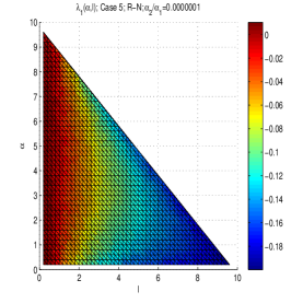
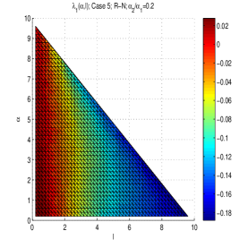
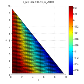
Figure 3.1: The relation among $\lambda_{1}(\alpha,l)$ and $\alpha$ and $l$ in Case 5. In the figures, “R-N” represents that the Robin boundary condition ($\alpha_{1}\varphi^{\prime}(0)-\alpha_{2}\varphi(0)=0$) is applied at $x=0$ and the Neumann boundary condition is applied at $x=L$. Here $f(u)=ru(1-u)$ and $g(u)=ru(1-u)(u-a)$. Parameters: $r=0.2$, $a=0.1$, $L=10$.

Theorem 3.9.

The following statements hold.

1. When Robin boundary condition ($\alpha_{1}\varphi^{\prime}(0)-\alpha_{2}\varphi(0)=0$) is applied at $x=0$ and Neumann boundary condition is applied at $x=L$, if $\alpha_{1}>0$, $\alpha_{2}>0$, and $\alpha_{2}/\alpha_{1}$ is sufficiently small, then the results in Theorem 3.1 are true; if $\alpha_{1}>0$, $\alpha_{2}>0$, and $\alpha_{2}/\alpha_{1}$ is sufficiently large, then the results in Theorem 3.7 are true.

2. When Robin boundary condition ($\alpha_{1}\varphi^{\prime}(0)-\alpha_{2}\varphi(0)=0$) is applied at $x=0$ and Dirichlet boundary condition is applied at $x=L$, if $\alpha_{1}>0$, $\alpha_{2}>0$, and $\alpha_{2}/\alpha_{1}$ is sufficiently small, then the results in Theorem 3.5 are true; if $\alpha_{1}>0$, $\alpha_{2}>0$, and $\alpha_{2}/\alpha_{1}$ is sufficiently large, then the results in Theorem 3.3 are true.

3. When Neumann boundary condition is applied at $x=0$ and Robin boundary condition ($\beta_{1}\varphi^{\prime}(L)+\beta_{2}\varphi(L)=0$) is applied at $x=L$, if $\beta_{1}>0$, $\beta_{2}>0$, and $\beta_{2}/\beta_{1}$ is sufficiently small, then the results in Theorem 3.1 are true; if $\beta_{1}>0$, $\beta_{2}>0$, and $\beta_{2}/\beta_{1}$ is sufficiently large, then the results in Theorem 3.5 are true.

4. When Dirichlet boundary condition is applied at $x=0$ and Robin boundary condition ($\beta_{1}\varphi^{\prime}(L)+\beta_{2}\varphi(L)=0$) is applied at $x=L$, if $\beta_{1}>0$, $\beta_{2}>0$, and $\beta_{2}/\beta_{1}$ is sufficiently small, then the results in Theorem 3.7 are true; if $\beta_{1}>0$, $\beta_{2}>0$, and $\beta_{2}/\beta_{1}$ is sufficiently large, then the results in Theorem 3.3 are true.

Figures 3.1 and 3.2 show the dependence of $\lambda_{1}(\alpha,l)$ on $\alpha$ and $l$ for different ratios of $\alpha_{2}/\alpha_{1}$ when Robin boundary condition ($\alpha_{1}\varphi^{\prime}(0)-\alpha_{2}\varphi(0)=0$) is applied at $x=0$ and Neumann or Dirichlet boundary condition is applied at $x=L$. The phenomena in the figures confirm the results in Theorem 3.9.

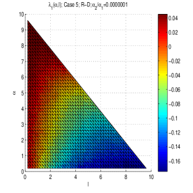
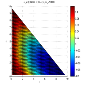
Figure 3.2: The relation among $\lambda_{1}(\alpha,l)$ and $\alpha$ and $l$ in Case 5. “R-D” represents that the Robin boundary condition ($\alpha_{1}\varphi^{\prime}(0)-\alpha_{2}\varphi(0)=0$) is applied at $x=0$ and the Dirichlet boundary condition is applied at $x=L$. Other parameters are the same as in Figure 3.1.

Figure 3.3 shows the time evolution of a solution of (1.4)-(1.5) under different boundary conditions and with different protection zone locations. It indicates that when the initial population density is low, the same setup of the protection zone may lead to population persistence or extinction under different boundary conditions and a different setup of the protection zone may help population persist in the whole domain even though the boundary conditions don’t change. In particular, with the parameters in Figure 3.3, we see that with the protection zone on the interval $[1,4]$ in the total habitat $[0,10]$, the population can persist if the boundary condition is Neumann at $x=0$ but it will be extinct if the boundary condition is Dirichlet at $x=0$; see Figure 3.3 (a-b) and (d-e). If the boundary condition is Dirichlet at $x=0$, then shifting the protection zone from the interval $[1,4]$ to the interval $[3,6]$ helps the population persist; see Figure 3.3 (b-c) and (e-f).

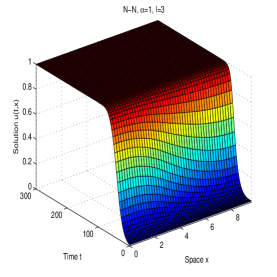
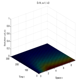
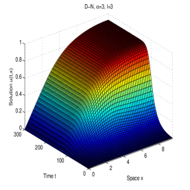
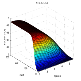
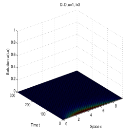
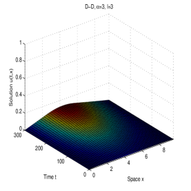
Figure 3.3: The solutions of (1.4)-(1.5) under different boundary conditions and with different protection zone locations. Other parameters are the same as in Figure 3.1. The initial conditions are $u_{0}(x)\equiv 0.01$.

4 Discussion

Designing effective strategies to protect an endangered species is important for the conservation of the species itself as well as the conservation of the habitat and the health of the involved ecosystems. Protection zones for an endangered or native species have been observed to provide many economic, social, environmental, and cultural values [28, 29, 3, 31, 36, 25]. Mathematical models have been developed to investigate the feasibility or efficiency of protection zones. Previous studies have been mainly focused on qualitative analysis and revealed that the size of a protection zone is always positively related to the persistence status of the population but when the size of the protection zone is small other factors such as the demographic or dispersal parameters also play important roles on the persistence of the population (see e.g., [19, 16, 18]).

In this work, we consider a reaction-diffusion model for a species in a one-dimensional bounded domain $[0,L]$. We assume that the growth of the species in its natural domain is subjected to a strong Allee effect, that is, its growth rate is negative when the population density is low, and hence, the population will not be able to recover once its density is below a certain level and the species will eventually be extinct. To protect the species, we assume that there is a protection zone $[\alpha,\alpha+l]$ in the habitat where the population’s growth satisfies a logistic type function and the population can grow to its carrying capacity there. We have proved that the principal eigenvalue $\lambda_{1}(\alpha,l)$ of the eigenvalue problem associated with the linearization of the system at the trivial solution can be used to determine population persistence ($\lambda_{1}(\alpha,l)<0$) and extinction ($\lambda_{1}(\alpha,l)>0$) (see Theorem 2.1). Our goal is to specify the relations between $\lambda_{1}(\alpha,l)$ and the parameters related to the protection zone and then provide precise strategies for an optimal protection zone in order for the population to persist.

It is not surprising to obtain that $\lambda_{1}(\alpha,l)$ is always a decreasing function of the length of the protection zone $l$ (see Lemma 3.1), which implies that the longer the protection zone is, the easier it is for the population to persist in the whole habitat. This is intuitively understandable and coincides with previous findings (see e.g., [19, 16, 18, 15]). The dependence of $\lambda_{1}(\alpha,l)$ on the starting point $\alpha$ of the protection zone is described in terms of the derivative of $\lambda_{1}(\alpha,l)$ with respect to $\alpha$, denoted by ${\lambda_{1}}_{\alpha}$, but the sign of ${\lambda_{1}}_{\alpha}$ is complicated and dependent of the boundary conditions. We study it in the cases of different combinations of Neumann and Dirichlet conditions. It turns out that ${\lambda_{1}}_{\alpha}$ is positive (resp. negative) for all $\alpha\in[0,L-l)$ if the boundary conditions are Neumann (at $x=0$)-Dirichlet (at $x=L$) (resp. Dirichlet-Neumann) and that ${\lambda_{1}}_{\alpha}$ is positive (resp. negative) first and then negative (resp. positive) when $\alpha$ increases from $0$ to $L-l$ if the boundary conditions are Neumann-Neumann (resp. Dirichlet-Dirichlet); see Lemmas 3.7, 3.8, 3.9, and 3.10.

By using the dependence of $\lambda_{1}(\alpha,l)$ on $\alpha$ and $l$, we then can investigate the effect of the protection zone on population persistence and extinction. In fact, if the growth rate in the protection zone is sufficiently large, then the population will persist in the whole domain in a long run regardless of the initial distribution and the location of the protection zone provided that the length of the protection zone is sufficiently large (see Theorems 3.2(i)(a), 3.4(i)(a), 3.6(i)(a), 3.8(i)(a)); if the growth rate in the protection zone is sufficiently small, then there are always initial data (typically all sufficiently small initial data) such that the population will be extinct no matter where the protection zone is or how long the protection zone is (see Theorems 3.4(ii), 3.6(iii), 3.8(iii)); otherwise, the population may persist when the protection zone is sufficiently long and is set up at some optimal locations (see Theorems 3.2((i)(b-1), (ii)(a)), 3.4(i)(b-1), 3.6((i)(b), (i)(c-1), (ii)), 3.8((i)(b), (i)(c-1), (ii))), while the population will be extinct if the protection zone is not long enough or is set up at a bad location (see Theorems 3.2((i)(b-2), (i)(c), (ii)(b)), 3.4((i)(b-2), (i)(c), (ii)), 3.6((i)(c-2), (i)(d), (ii)), 3.8((i)(c-2), (i)(d), (ii))). Note that in this paper, by “extinction”, we mean that the population will be extinct if its initial distribution density is sufficiently low. By comparing these results, we see that, in general, if there is a Neumann boundary end, then the optimal location for the protection zone, if needed, is the part of the domain connecting the Neumann boundary end; if both ends are Dirichlet, then the optimal location for the protection zone, if needed, should be in the middle of the domain. Due to the mathematical complexity rising in the cases of Robin boundary conditions, we have not obtained all detailed results about the optimal locations for the protection zone in these cases, but we have seen that if the Robin boundary condition is more like a Neumann (or Dirichlet) condition, then the results related to the system is more like those related to the system with a Neumann (or Dirichlet) condition.

We complete this paper by proposing several interesting problems that deserve further consideration. The first one is to extend the study of the effects of protection zones on spatial population dynamics to the time-periodic setting. Many plant and animal species have demonstrated seasonal population dynamics in response to seasonal fluctuations and time-periodic varying environments, in particular, the weather conditions [47]. The spatiotemporal environments play an important role in characterizing the persistence and extinction of some species, such as diseases transmission [2, 40, 50], single population growth [8]. Some plants may become extinct in arid seasons, while vegetate densely in moist climate, so it is interesting to investigate how protection zones can prevent population from extinction though the species lives in some arid seasons. Another issue is to concern the protection mechanism in a network. A real river system usually has rich topological structures, which greatly influence the population growth and spread of organisms living in it [6]. It is spontaneous and crucial to prevent endangered species in real river systems from extinction. From a mathematical point of view, the addition of advection to reaction-diffusion models may change the long term outcome (persistence/extinction) of the population [30, 32] in river systems. Based on a local river reaction-diffusion equation, [33, 17, 41] studied the dynamical behavior of species spreading from a location in a river network where two or three branches meet. It has been found that both the water flow speeds in the river branches and the cross section areas can affect the extinction/persistence of species. Nevertheless, to our knowledge, there hasn’t been any understanding about the long-term population dynamics when a protection measure is considered to ensure the perpetual persistence in a river network. This should also be an interesting problem for future work.

5 Appendix

5.1 Proof of Lemma 3.5

Assume that (H2) is true, i.e., $g^{\prime}(0)+\lambda_{1}(\alpha,l)=0.$ We can write the general form of $\varphi_{1}$ in (3.1) on $[0,L]$ as

$$\varphi_{1}(x)=\left\{\begin{array}[]{ll}C_{3}+C_{4}x,&\text{for}\;\;x\in[0,\alpha],\\ C_{1}\cos\tilde{f}x+C_{2}\sin\tilde{f}x,&\text{for}\;\;x\in[\alpha,\alpha+l],\\ C_{5}+C_{6}x,&\text{for}\;\;x\in[\alpha+l,L],\end{array}\right.$$ (5.1)

where each $C_{i}$ ($i=1,\cdots,6$) is a constant. Then

$$\varphi_{1}^{\prime}(x)=\left\{\begin{array}[]{ll}C_{4},&\text{for}\;\;x\in[0,\alpha],\\ -C_{1}{\tilde{f}}\sin\tilde{f}x+C_{2}{\tilde{f}}\cos\tilde{f}x,&\text{for}\;\;x\in[\alpha,\alpha+l],\\ C_{6},&\text{for}\;\;x\in[\alpha+l,L].\end{array}\right.$$

We first consider the case where the Dirichlet boundary condition is applied at $x=0$ and $x=L$. The boundary conditions of $\varphi_{1}$ at $0$ and $L$ lead to

$$\begin{array}[]{l}-\alpha_{2}C_{3}=0,\quad\beta_{2}(C_{5}+C_{6}L)=0,\end{array}$$

which imply $C_{3}=0$ and $C_{6}=-C_{5}/L$. Due to the continuous differentiability of $\varphi_{1}$ at $\alpha$ and $\alpha+l$, we infer that

$$C_{4}\alpha=C_{1}\cos\tilde{f}\alpha+C_{2}\sin\tilde{f}\alpha,$$ (5.2)

$$C_{4}=-C_{1}{\tilde{f}}\sin\tilde{f}\alpha+C_{2}{\tilde{f}}\cos\tilde{f}\alpha,$$ (5.3)

$$C_{5}-C_{5}(\alpha+l)/L=C_{1}\cos\tilde{f}(\alpha+l)+C_{2}\sin\tilde{f}(\alpha+l),$$ (5.4)

$$-C_{5}/L=-C_{1}{\tilde{f}}\sin\tilde{f}(\alpha+l)+C_{2}{\tilde{f}}\cos\tilde{f}(\alpha+l).$$ (5.5)

Then $\eqref{RR1ap}\times\eqref{RR2ap}+\dfrac{\eqref{RR3ap}\times\eqref{RR4ap}}{\tilde{f}^{2}}$ leads to

$$\begin{array}[]{l}\displaystyle C_{4}C_{5}(\alpha(1-\frac{\alpha+l}{L})-\frac{1}{L\tilde{f}^{2}})=(C_{1}^{2}+C_{2}^{2})\cos{\tilde{f}}l\end{array}$$ (5.6)

and $\eqref{RR1ap}\times\eqref{RR4ap}-\eqref{RR3ap}\times\eqref{RR2ap}$ leads to

$$\begin{array}[]{l}C_{4}C_{5}(-\frac{\alpha}{L}-(1-\frac{\alpha+l}{L}))=-(C_{1}^{2}+C_{2}^{2}){\tilde{f}}\sin{\tilde{f}}l.\end{array}$$ (5.7)

By simplifying (5.6) and (5.7), we obtain that $\lambda_{1}(\alpha,l)$ satisfies (3.19). Differentiating (3.19) with respect $\alpha$ on two sides yields

$$\begin{array}[]{rcl}&&\sec^{2}{\tilde{f}}l\cdot l\cdot\displaystyle\frac{\lambda_{1\alpha}}{2\tilde{f}}\\ &=&\displaystyle\frac{(L-l)\frac{\lambda_{1\alpha}}{2\tilde{f}}({\tilde{f}}^{2}\alpha(L-\alpha-l)-1)-(L-l){\tilde{f}}(2{\tilde{f}}\frac{\lambda_{1\alpha}}{2\tilde{f}}\alpha(L-\alpha-l)+{\tilde{f}}^{2}(L-\alpha-l)-{\tilde{f}}^{2}\alpha)}{T_{2}^{2}},\end{array}$$

which gives (3.20).

We next consider the case where the Neumann boundary condition is applied at $x=0$ and the Dirichlet boundary condition is applied at $x=L$. The boundary conditions of $\varphi_{1}$ at $0$ and $L$ infer

$$\begin{array}[]{l}\alpha_{1}C_{4}=0,\quad\beta_{2}(C_{5}+C_{6}L)=0,\end{array}$$

which imply $C_{4}=0$ and $C_{6}=-C_{5}/L$. As $\varphi_{1}$ is continuously differentiable at $\alpha$ and $\alpha+l$, we have

$$C_{3}=C_{1}\cos\tilde{f}\alpha+C_{2}\sin\tilde{f}\alpha,$$ (5.8)

$$0=-C_{1}{\tilde{f}}\sin\tilde{f}\alpha+C_{2}{\tilde{f}}\cos\tilde{f}\alpha,$$ (5.9)

$$C_{5}-C_{5}(\alpha+l)/L=C_{1}\cos\tilde{f}(\alpha+l)+C_{2}\sin\tilde{f}(\alpha+l),$$ (5.10)

$$-C_{5}/L=-C_{1}{\tilde{f}}\sin\tilde{f}(\alpha+l)+C_{2}{\tilde{f}}\cos\tilde{f}(\alpha+l).$$ (5.11)

Then $\eqref{RR1apND}\times\eqref{RR2apND}+\dfrac{\eqref{RR3apND}\times\eqref{RR4apND}}{\tilde{f}^{2}}$ leads to

$$\begin{array}[]{l}\displaystyle C_{3}C_{5}(1-\frac{\alpha+l}{L})=(C_{1}^{2}+C_{2}^{2})\cos{\tilde{f}}l\end{array}$$ (5.12)

and $\eqref{RR1apND}\times\eqref{RR4apND}-\eqref{RR3apND}\times\eqref{RR2apND}$ leads to

$$\begin{array}[]{l}-C_{3}C_{5}\frac{1}{L}=-(C_{1}^{2}+C_{2}^{2}){\tilde{f}}\sin{\tilde{f}}l.\end{array}$$ (5.13)

By simplifying (5.12) and (5.13), we obtain that $\lambda_{1}(\alpha,l)$ satisfies (3.21). Differentiating (3.21) with respect $\alpha$ on two sides yields

$$\begin{array}[]{rcl}\sec^{2}{\tilde{f}}l\cdot l\cdot\frac{\lambda_{1\alpha}}{2\tilde{f}}=\frac{1}{(L-\alpha-l)^{2}}\frac{1}{\tilde{f}}-\dfrac{1}{L-\alpha-l}\frac{\lambda_{1\alpha}}{2\tilde{f}^{3}},\end{array}$$

which implies (3.22) immediately.

5.2 Proof of Lemma 3.6

Assume that (H3) is true, i.e., $g^{\prime}(0)+\lambda_{1}(\alpha,l)>0.$ We can write the general form of $\varphi_{1}$ on $[0,L]$ as

$$\varphi_{1}(x)=\left\{\begin{array}[]{ll}C_{3}\cos\tilde{g}x+C_{4}\sin\tilde{g}x,&\text{for}\;\;x\in[0,\alpha],\\ C_{1}\cos\tilde{f}x+C_{2}\sin\tilde{f}x,&\text{for}\;\;x\in[\alpha,\alpha+l],\\ C_{5}\cos\tilde{g}x+C_{6}\sin\tilde{g}x,&\text{for}\;\;x\in[\alpha+l,L],\end{array}\right.$$ (5.14)

where each $C_{i}$ ($i=1,\cdots,6$) is a constant. Then it holds that

$$\varphi_{1}^{\prime}(x)=\left\{\begin{array}[]{ll}-C_{3}{\tilde{f}}\sin\tilde{f}x+C_{4}{\tilde{f}}\cos\tilde{f}x,&\text{for}\;\;x\in[0,\alpha],\\ -C_{1}{\tilde{f}}\sin\tilde{f}x+C_{2}{\tilde{f}}\cos\tilde{f}x,&\text{for}\;\;x\in[\alpha,\alpha+l],\\ -C_{5}{\tilde{f}}\sin\tilde{f}x+C_{6}{\tilde{f}}\cos\tilde{f}x,&\text{for}\;\;x\in[\alpha+l,L].\end{array}\right.$$

We first consider the case where the Dirichlet boundary condition is applied at $x=0$ and $x=L$. By the boundary conditions of $\varphi_{1}$ at $0$ and $L$, we have

$$\begin{array}[]{l}C_{3}=0,\quad C_{5}\cos{\tilde{g}}L+C_{6}\sin{\tilde{g}}L=0,\end{array}$$

which imply $C_{6}=-\cot{\tilde{g}}L\cdot C_{5}$. Using the continuous differentiability of $\varphi_{1}$ at $\alpha$ and $\alpha+l$, we obtain

$$C_{4}\sin{\tilde{g}}\alpha=C_{1}\cos\tilde{f}\alpha+C_{2}\sin\tilde{f}\alpha,$$ (5.15)

$$C_{4}{\tilde{g}}\cos{\tilde{g}}\alpha=-C_{1}{\tilde{f}}\sin\tilde{f}\alpha+C_{2}{\tilde{f}}\cos\tilde{f}\alpha,$$ (5.16)

$$C_{5}\cos{\tilde{g}}(\alpha+l)-\cot{\tilde{g}}L\cdot C_{5}\sin{\tilde{g}}(\alpha+l)=C_{1}\cos\tilde{f}(\alpha+l)+C_{2}\sin\tilde{f}(\alpha+l),$$ (5.17)

$$-C_{5}\tilde{g}\sin{\tilde{g}}(\alpha+l)-\cot{\tilde{g}}L\cdot C_{5}{\tilde{g}}\cos{\tilde{g}}(\alpha+l)=-C_{1}{\tilde{f}}\sin\tilde{f}(\alpha+l)+C_{2}{\tilde{f}}\cos\tilde{f}(\alpha+l).$$ (5.18)

Then $\eqref{RR1H3apdd}\times\eqref{RR2H3apdd}+\dfrac{\eqref{RR3H3apdd}\times\eqref{RR4H3apdd}}{\tilde{f}^{2}}$ leads to

$$\begin{array}[]{rl}&C_{4}C_{5}\Big{[}\sin{\tilde{g}}\alpha(\cos{\tilde{g}}(\alpha+l)-\cot{\tilde{g}}L\cdot\sin{\tilde{g}}(\alpha+l))-\displaystyle\frac{{\tilde{g}}\cos{\tilde{g}}\alpha(\tilde{g}\sin{\tilde{g}}(\alpha+l)-\cot{\tilde{g}}L\cdot{\tilde{g}}\cos{\tilde{g}}(\alpha+l))}{{\tilde{f}}^{2}}\Big{]}\\ &=(C_{1}^{2}+C_{2}^{2})\cos{\tilde{f}}l\end{array}$$ (5.19)

and $\eqref{RR1H3apdd}\times\eqref{RR4H3apdd}-\eqref{RR3H3apdd}\times\eqref{RR2H3apdd}$ leads to

$$\begin{array}[]{rl}&-C_{4}C_{5}(\sin{\tilde{g}}\alpha(\tilde{g}\sin{\tilde{g}}(\alpha+l)+\cot{\tilde{g}}L\cdot{\tilde{g}}\cos{\tilde{g}}(\alpha+l))+{\tilde{g}}\cos{\tilde{g}}\alpha(\cos{\tilde{g}}(\alpha+l)-\cot{\tilde{g}}L\cdot C_{5}\sin{\tilde{g}}(\alpha+l)))\\ &=-(C_{1}^{2}+C_{2}^{2}){\tilde{f}}\sin{\tilde{f}}l.\end{array}$$ (5.20)

By simplifying (5.19) and (5.20), we see that (3.23) holds. Differentiating (3.23) with respect $\alpha$ on two sides, we get (3.24).

We next consider the case where the Neumann boundary condition is applied at $x=0$ and the Dirichlet boundary condition is applied at $x=L$. In view of the boundary conditions of $\varphi_{1}$ at $0$ and $L$, we find

$$\begin{array}[]{l}C_{4}=0,\quad C_{5}\cos{\tilde{g}}L+C_{6}\sin{\tilde{g}}L=0,\end{array}$$

which imply $C_{6}=-\cot{\tilde{g}}L\cdot C_{5}$. Thanks to the continuous differentiability of $\varphi_{1}$ at $\alpha$ and $\alpha+l$, we see

$$C_{3}\cos{\tilde{g}}\alpha=C_{1}\cos\tilde{f}\alpha+C_{2}\sin\tilde{f}\alpha,$$ (5.21)

$$-C_{3}{\tilde{g}}\sin{\tilde{g}}\alpha=-C_{1}{\tilde{f}}\sin\tilde{f}\alpha+C_{2}{\tilde{f}}\cos\tilde{f}\alpha,$$ (5.22)

$$C_{5}\cos{\tilde{g}}(\alpha+l)-\cot{\tilde{g}}L\cdot C_{5}\sin{\tilde{g}}(\alpha+l)=C_{1}\cos\tilde{f}(\alpha+l)+C_{2}\sin\tilde{f}(\alpha+l),$$ (5.23)

$$-C_{5}\tilde{g}\sin{\tilde{g}}(\alpha+l)-\cot{\tilde{g}}L\cdot C_{5}{\tilde{g}}\cos{\tilde{g}}(\alpha+l)=-C_{1}{\tilde{f}}\sin\tilde{f}(\alpha+l)+C_{2}{\tilde{f}}\cos\tilde{f}(\alpha+l).$$ (5.24)

Then $\eqref{RR1H3apnd}\times\eqref{RR2H3apnd}+\dfrac{\eqref{RR3H3apnd}\times\eqref{RR4H3apnd}}{\tilde{f}^{2}}$ leads to

$$\begin{array}[]{rl}&C_{3}C_{5}\Big{[}\cos{\tilde{g}}\alpha(\cos{\tilde{g}}(\alpha+l)-\cot{\tilde{g}}L\cdot\sin{\tilde{g}}(\alpha+l))+\displaystyle\frac{{\tilde{g}}\sin{\tilde{g}}\alpha(\tilde{g}\sin{\tilde{g}}(\alpha+l)+\cot{\tilde{g}}L\cdot{\tilde{g}}\cos{\tilde{g}}(\alpha+l))}{{\tilde{f}}^{2}}\Big{]}\\ &=(C_{1}^{2}+C_{2}^{2})\cos{\tilde{f}}l,\end{array}$$ (5.25)

and $\eqref{RR1H3apnd}\times\eqref{RR4H3apnd}-\eqref{RR3H3apnd}\times\eqref{RR2H3apnd}$ leads to

$$\begin{array}[]{rl}&C_{3}C_{5}(-\cos{\tilde{g}}\alpha(\tilde{g}\sin{\tilde{g}}(\alpha+l)-\cot{\tilde{g}}L\cdot{\tilde{g}}\cos{\tilde{g}}(\alpha+l))+{\tilde{g}}\sin{\tilde{g}}\alpha(\cos{\tilde{g}}(\alpha+l)-\cot{\tilde{g}}L\cdot C_{5}\sin{\tilde{g}}(\alpha+l)))\\ &=-(C_{1}^{2}+C_{2}^{2}){\tilde{f}}\sin{\tilde{f}}l.\end{array}$$ (5.26)

By simplifying (5.25) and (5.26), we obtain (3.25). Differentiating (3.25) with respect $\alpha$ on two sides gives rise to (3.26).

References

• [1] W. C. Allee, Animal aggregations. A study in general sociology. University of Chicago Press, Chicago, 1931.
• [2] L. J. Allen, B. M. Bolker, Y. Lou, A. L. Nevai, Asymptotic profiles of the steady states for an SIS epidemic reaction-diffusion model, Discrete Continuous Dynamical Systems A, 21(2008), 1-20.
• [3] D. Ami, P. Cartigny, A. Rapaport, Can marine protected areas enhance both economic and biological situations? Comptes Rendus, Biologies, 328(2005), 357-366.
• [4] J. von Below, Classical solvability of linear parabolic equations on networks, Journal of Differential Equations, 72(1988) 316-337.
• [5] J. S. Brashares, J. R. Werner, A. R. E. Sinclair, Social “meltdown” in the demise of an island endemic: Allee effects and the Vancouver Island marmot, Journal of Animal Ecology, 79(5)(2010), 965-973.
• [6] E. H. Campbell Grant, W. H. Lowe, W. F. Fagan, Living in the branches: population dynamics and ecological processes in dendritic networks, Ecology Letters, 10(2)(2007), 165-175.
• [7] R. S. Cantrell, C. Cosner, Spatial Ecology Via Reaction-Diffusion Equations, Wiley Series in Mathematical and Computational Biology. John Wiley Sons Ltd., Chichester, 2003.
• [8] R. S. Cantrell, C. Cosner, Diffusive logistic equations with indefinite weights: population models in disrupted environments, Proceedings of the Royal Society of Edinburgh Section A, 112(1989), 293-318.
• [9] X. Chang, J. Wei, Stability and Hopf bifurcation in a diffusive predator-prey system incorporating a prey refuge, Mathematical Biosciences and Engineering, 10(4)(2013), 979-996.
• [10] F. Courchamp, L. Berec, J. Gascoigne, Allee effects in ecology and conservation, Oxford University Press, Oxford, 2008.
• [11] R. Cui, J. Shi, B. Wu, Strong Allee effect in a diffusive predator-prey system with a protection zone, Journal of Differential Equations, 256(2014), 108-129.
• [12] R. Cui, H. Li, L. Mei, J. Shi, Effect of harvesting quota and protection zone in a reaction-diffusion model arising from fishery management, Discrete and Continuous Dynamical Systems B, 22(2017), 791-807.
• [13] A. M. De Roos, L. Persson, Size-dependent life-history traits promote catastrophic collapses of top predators, Proceedings of the National Academy of Sciences USA, 99(20)(2002), 12907-12912.
• [14] N. T. Dieu, N. H. Du, H. D. Nguyen, G. Yin, Protection zones for survival of species in random environment, SIAM Journal on Applied Mathematics, 76(2016), 1382-1402.
• [15] K. Du, R. Peng, N. Sun, The role of protection zone on species spreading governed by a reactio diffusion model with strong Allee effect, Journal of Differential Equations, 266(2019), 7327-7356.
• [16] Y. Du, X. Liang, A diffusive competition model with a protection zone, Journal of Differential Equations, 244 (2008), 61-86.
• [17] Y. Du, B. D. Lou, R. Peng, M. L. Zhou, The Fisher-KPP equation over simple graphs: varied persistence states in river networks, Journal of Mathematical Biology, 80(2020), 1559-1616.
• [18] Y. Du, R. Peng, M. Wang, Effect of a protection zone in the diffusive Leslie predator-prey model, Journal of Differential Equations, 246(2009), 3932-3956.
• [19] Y. Du, J. Shi, A diffusive predator-prey model with a protection zone, Journal of Differential Equations, 229(2006), 63-91.
• [20] Y. Du, J. Shi, Some recent results on diffusive predator-prey models in spatially heterogeneous environment, in: Nonlinear Dynamics and Evolution Equations, in: Fields Institute Communications, vol.48, American Mathematical Society, Providence, RI, 2006, pp.95-135.
• [21] M. Fan, K. Wang, Y. Zhang, S. Zhang, H. Liu, Study on harvested population with diffusional maigration, Journal of Systems Science and Complexity, 14(2)(2001), 139-148.
• [22] D. Gao, X. Liang, A competition-diffusion system with a refuge, Discrete and Continuous Dynamical Systems B, 8(2007), 435-454.
• [23] J. Gascoigne, R. N. Lipcius, Allee effects in marine systems, Marine Ecology Progress Series, 269(2004), 49-59.
• [24] J. Hale, Asymptotic behavior of dissipative systems, American Mathematical Society Providence, RI, 1988.
• [25] B. Halpern, The impact of marine reserves: Do reserves work and does reserve size matter? Ecological Applications, 13(sp1)(2003), 117-137.
• [26] X. He, S. Zheng, Protection zone in a diffusive predator-prey model with Beddington-DeAngelis functional response, Journal of Mathematical Biology, 75(2017), 239-257.
• [27] P. Hess, Periodic-Parabolic Boundary Value Problems and Positivity, Pitman Search Notes in Mathematics Series, vol.247, Longman Scientific Technical, Harlow, UK, 1991.
• [28] R. D. Holt, Predation, apparent competition, and the structure of prey communities, Theoretical Population Biology, 12(1977), 197-229.
• [29] R. D. Holt, Spatial heterogeneity, indirect interactions, and the coexistence of prey species, The American Naturalist, 124(1984), 377-406.
• [30] S.-B. Hsu, Y. Lou, Single phytoplankton species growth with light and advection in a water column, SIAM Journal on Applied Mathematics, 70(8)(2010), 2942-2974.
• [31] M. Jerry, A. Rapaport, P. Cartigny, Can protected areas potentially enlarge viability domains for harvesting management? Nonlinear Analysis: Real World Applications, 11(2010), 720-734.
• [32] Y. Jin, M. A. Lewis, Seasonal influences on population spread and persistence in streams: critical domain size, SIAM Journal on Applied Mathematics, 71(4)(2011), 1241-1262.
• [33] Y. Jin, R. Peng, J. Shi, Population dynamics in river networks, Journal of Nonlinear Science, 29(2019), 2501-2545.
• [34] T. H. Keitt, M. A. Lewis, R. D. Holt, Allee effects, invasion pinning, and species’ borders, The American Naturalist, 157(2)(2001), 203-216.
• [35] S. Li, J. Wu, S. Liu, Effect of cross-diffusion on the stationary problem of a Leslie prey-predator model with a protection zone, Calculus of Variations & Partial Differential Equations, 56, 82(2017).
• [36] P. Loisel, P. Cartigny, How to model marine reserves? Nonlinear Analysis: Real World Applications, 10(2009), 1784-1796.
• [37] W. Ni, M. Wang, Dynamics and patterns of a diffusive Leslie-Gower prey-predator model with strong Allee effect in prey, Journal of Differential Equations, 261(2016), 4244-4274.
• [38] K. Oeda, Effect of cross-diffusion on the stationary problem of a prey-redator model with a protection zone, Journal of Differential Equations, 250(2011), 3988-4009.
• [39] S. Oruganti, J. Shi, R. Shivaji, Diffusive logistic equation with constant yield harvesting. I. Steady states, Transactions of the American Mathematical Society, 354(9)(2002), 3601-3619.
• [40] R. Peng, X.-Q. Zhao, A reaction-diffusion SIS epidemic model in a time-periodic environment, Nonlinearity, 25(2012), 1451-1471.
• [41] J. M. Ramirez, Population persistence under advection-diffusion in river networks, Journal of mathematical biology, 65(5)(2012), 919-942.
• [42] J. Shi, R. Shivaji, Persistence in reaction diffusion models with weak Allee effect, Journal of Mathematical Biology, 52(6)(2006), 807-829.
• [43] H. L. Smith, X.-Q. Zhao, Robust persistence for semidynamical systems, Nonlinear Analysis, Theory, Methods and Applications, 47(2001), 6169-6179.
• [44] N. Sun, C. Lei, Long-time behavior of a reaction-diffusion model with strong Allee effect and free boundary: Effect of protection zone, (2019), arXiv:1912.10451.
• [45] N. Sun, X. Han, Asymptotic behavior of solutions of a reaction-diffusion model with a protection zone and a free boundary, Applied Mathematics Letters, 107(2020), 106470.
• [46] J. Tripathi, S. Abbas, M. Thakur, A density dependent delayed predator-prey model with Beddington-DeAngelis type Function Response incorporating a prey refuge, Communications in Nonlinear Science and Numerical Simulation, 22(2015), 427-450.
• [47] J. Wang, N. H. Ogden, H. Zhu, The impact of weather conditions on Culex pipiens and Culex restuans (Diptera: Culicidae) abundance: a case study in Peel region, Journal of Medical Entomology, 48(2)(2011), 468-475.
• [48] J. F. Wang, J. P. Shi, J. J. Wei, Predator-prey system with strong Allee effect in prey, Journal of Mathematical Biology, 63(2011), 291-331.
• [49] J. F. Wang, J. P. Shi, J. J. Wei, Dynamics and pattern formation in a diffusive predator-prey system with strong Allee effect in prey, Journal of Differential Equations, 251(2011), 1276-1304.
• [50] W. D. Wang, X. Q. Zhao, Threshold dynamics for compartmental epidemic models in periodic environments, Journal of Dynamics and Differential Equations, 20(2008), 699-717.
• [51] Y. Wang, W. Li, Effect of cross-diffusion on the stationary problem of a diffusive competition model with a protection zone, Nonlinear Analysis: Real World Applications, 14(2013), 224-245.
• [52] Y. Wang, J. Shi, Analysis of a reaction-diffusion benthic-drift model with strong Allee effect growth, Journal of Differential Equations, 269(2020), 7605-7642.
• [53] Y. Wang, J. Shi, Persistence and extinction of population in reaction-diffusion-advection model with weak Allee effect growth, SIAM Journal on Applied Mathematics, 79(4)(2019), 1293-1313.
• [54] Y. Wang, J. Shi, J. Wang, Persistence and extinction of population in reaction-diffusion-advection model with strong Allee effect growth, Journal of Mathematical Biology, 78(7)(2019), 2093-2140.
• [55] X. Zou, K. Wang, The protection zone of biological population, Nonlinear Analysis: Real World Applications, 12(2011), 956-964.