Random phase approximation with exchange for an accurate description of
crystalline polymorphism

Abstract

We determine the correlation energy of BN, SiO₂ and ice polymorphs employing a recently developed RPAx (random phase approximation with exchange) approach. The RPAx provides larger and more accurate polarizabilities as compared to the RPA, and captures effects of anisotropy. In turn, the correlation energy, defined as an integral over the density-density response function, gives improved binding energies without the need for error cancellation. Here, we demonstrate that these features are crucial for predicting the relative energies between low- and high-pressure polymorphs of different coordination number as, e.g., between $\alpha$-quartz and stishovite in SiO₂, and layered and cubic BN. Furthermore, a reliable (H₂O)₂ potential energy surface is obtained, necessary for describing the various phases of ice. The RPAx gives results comparable to other high-level methods such as coupled cluster and quantum Monte Carlo, also in cases where the RPA breaks down. Although higher computational cost than RPA we observe a faster convergence with respect to the number of eigenvalues in the response function.

I Introduction

The development of an accurate, yet computationally efficient, electronic structure approach able to treat electron correlation in solids remains an important task in condensed matter physics. Density functional theory (DFT) provides a rigorous and computationally appealing framework Hohenberg and Kohn (1964); Kohn and Sham (1965) that has been widely successful, but available approximations still suffer a number of drawbacks. The van der Waals (vdW) interactions, ubiquitous in systems ranging from layered materials to superconducting hydrides, are challenging to include Björkman et al. (2012), and most exchange-correlation (xc) functionals do not achieve the accuracy needed to satisfactorily describe the energetics of phase transformations and polymorphism, even in common systems like water Gillan et al. (2016) and silica Hay et al. (2015).

The random phase approximation (RPA) represents the highest level of sophistication currently applied in materials science Nguyen and de Gironcoli (2009); Harl and Kresse (2009); Ren et al. (2012). Being based on the exact adiabatic-connection fluctuation-dissipation (ACFD) formula Langreth and Perdew (1975); Stromsheim et al. (2011), first-order Hartree-Fock exchange is exactly incorporated and vdW forces are seamlessly built in, providing an overall improved accuracy. However, the performance of the RPA strongly relies on error cancellation, leading to unpredictable errors when dealing with crystals of low symmetry Xiao et al. (2012); Sengupta et al. (2018). Futhermore, vdW forces are underestimated by an average of 20% Zhu et al. (2010); Dixit et al. (2017); Hellgren et al. (2018). The origin of these errors can, however, easily be traced to the approximate Hartree response function used for constructing the correlation energy.

The combination of the ACFD formula and time-dependent (TD) DFT has opened a path for systematic improvements of the RPA Lein et al. (2000); Marques et al. (2006). Within TDDFT, xc effects are incorporated via the xc kernel that can be defined as the second density variation of the xc action functional Gross and Kohn (1985); van Leeuwen (1998); von Barth et al. (2005). Starting from the RPA, i.e., the Hartree kernel, further refinements then naturally proceed via the local density approximation (LDA) and generalized gradient approximations (GGAs). However, first results found that these approximations can worsen the performance with respect to the RPA Furche and Van Voorhis (2005). A renormalized LDA kernel that introduces spacial nonlocality was, therefore, formulated in Ref. Olsen and Thygesen (2012). This kernel, as well as a renormalized PBE (Perdew-Burke-Ernzerhof) kernel, have shown to improve the RPA correlation energy, leading to a better performance in several cases Olsen and Thygesen (2014); Sengupta et al. (2018); Olsen et al. (2019).

Within an approach that combines many-body perturbation theory (MBPT) and TDDFT the first step beyond RPA is to include the full Fock exchange term in the density response function via the nonlocal and frequency dependent exact-exchange (EXX) kernel. This generates the random phase approximation with exchange (RPAx), that exactly includes the second order exchange diagram as well as higher order exchange effects, in addition to the RPA ring series of diagrams Fetter and Walecka (2003); Görling (1998); Hellgren and von Barth (2008, 2010); elmann and Görling (2010). Various partial resummations of the RPAx correlation terms are thus equal to other advanced expressions for the correlation energy defined within MBPT such as, e.g., SOSEX (second order screened exchange) Freeman (1977); Grüneis et al. (2009); Jansen et al. (2010); Ren et al. (2013); Colonna et al. (2014); Hellgren et al. (2018). First tests on atoms and molecules have shown that not only accurate correlation energies are obtained with RPAx Colonna et al. (2016); Hellgren et al. (2018), but also xc potentials, i.e., electronic densities, and polarisabilities Hellgren and von Barth (2010); Bleiziffer et al. (2015). Furthermore, studies on the homogeneous electron gas, the simplest model of a metal, have shown promising results Colonna et al. (2014).

In this work, we extend the scope of applications to solids and show that it is possible to reach results of similar quality as for molecules. We calculate the relative energies between various crystalline phases within the BN, SiO₂ and ice polymorphs. In particular, we investigate cases where the RPA has shown insufficient, as, e.g., for the $\alpha$-quartz-stishovite energy difference in SiO₂, for which the change in coordination number necessitate accurate correlation energies Xiao et al. (2012); Hay et al. (2015); Sengupta et al. (2018). A similar problem occurs in cubic and layered BN, inverting their stability order Cazorla and Gould (2019); Gruber and Grüneis (2018). In both SiO₂ and BN the vdW forces play an important role Marini et al. (2006); Björkman et al. (2012); Hay et al. (2015). Here we investigate the effect of the EXX kernel on the binding energy of layered BN as well as the energy difference between $\alpha$-quartz and cristobalite. A study of purely vdW bonded solids, such as Ar and Kr, confirms that the vdW bond is well described with RPAx, yielding an accuracy similar to that found for molecular dimers. Finally, we perform a detailed analysis of the water dimer potential energy surface and ice polymorphism. The delicate balance between Pauli repulsion, static and dynamic correlation has made water a long-standing problem for electronic structure methods.

Our results on this broad and challenging set of systems show promise for future applications. The RPAx stays within the simple computational framework of the RPA, but has an accuracy comparable with more sophisticated methods such as quantum Monte Carlo (QMC) and coupled cluster (CC).

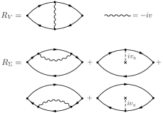
Figure 1: Diagrammatic representation of the two terms in Eq. (4). Full lines correspond to KS Green functions.

II RPA with exchange

In this section we summarize the equations of the RPAx approximation for periodic solids. These have been introduced previously Hellgren and von Barth (2008, 2010) but are here adapted to the specific implementation employed in this work Colonna et al. (2014, 2016); Hellgren et al. (2018).

The RPAx approximation for the correlation energy is based on the ACFD (adiabatic connection fluctuation-dissipation) formula, in which the exact correlation energy is expressed in terms of the linear density response function, $\chi_{\lambda}$, multiplied by the Coulomb interaction, $v$, and integrated over the frequency and the interaction strength $\lambda$

$$E_{\rm c}=-\int_{0}^{1}d\lambda\int_{0}^{\infty}\frac{d\omega}{2\pi}{\rm Tr}\{v[\chi_{\lambda}(i\omega)-\chi_{s}(i\omega)]\}.$$ (1)

The underlying Hamiltonian is given by

$$H=T+V^{\lambda}+\lambda W,$$ (2)

where $T$ is the kinetic energy operator, $W$ is the electron-electron interaction operator, and $V^{\lambda}$ is a one-body potential operator composed of the external potential and a fictitious potential that fix the density at full interaction strength for every $\lambda$. With this definition, the system at $\lambda=0$ already produces the exact density, $n$, via the exact Kohn-Sham (KS) xc potential, $v_{\rm xc}$. The KS independent-particle response function, subtracted in Eq. (1), is denoted $\chi_{s}$.

Within TDDFT, $\chi_{\lambda}$ becomes a functional of the ground-state density, $n_{0}$, via the xc kernel, $f^{\lambda}_{\rm xc}=\delta v^{\lambda}_{\rm xc}/\delta n|_{n_{0}}$. This can be expressed in a Dyson-like equation

$$\chi_{\lambda}(\omega)=\chi_{s}(\omega)+\chi_{s}(\omega)[\lambda v+f^{\lambda}_{\rm xc}(\omega)]\chi_{\lambda}(\omega),$$ (3)

similar to the RPA (or Hartree) equation ($f_{\rm xc}=0$).

A systematic approach for generating xc kernels based on many-body perturbation theory was introduced in Ref. von Barth et al., 2005. Within this approach the simplest approximation corresponds to including the full Fock exchange term via a time-dependent optimized effective potential scheme. This results in the EXX kernel, $f_{\rm x}$, defined by the following equation

$$\chi_{s}(\omega)f_{\rm x}(\omega)\chi_{s}(\omega)=R_{V}(\omega)+R_{\Sigma}(\omega).$$ (4)

The right hand side can be interpreted diagrammatically in terms of KS Green functions, being the sum of the first order vertex diagram, $R_{V}(\omega)$, and the first order self-energy correction diagrams $R_{\Sigma}(\omega)$ (see Fig. 1). Although $f_{\rm x}$ is first order in the Coulomb interaction, the correlation energy, via Eq. (1), contains all orders in $v$. This approximation to the correlation energy is what we call RPAx and is the same as the one used in Ref. elmann and Görling (2010). Other variants based on a dielectric formulation Mussard et al. (2016), or Hartree-Fock orbitals and range-separation have also been proposed Toulouse et al. (2009). We emphasize that the RPAx, as defined here, is based on TDDFT and KS orbitals, thus falling in the category of orbital functionals in DFT (i.e. functionals depending on the (un)occupied KS orbitals and eigenvalues). The total energy functional can then be minimized via a local KS potential in the usual way Hellgren and von Barth (2010).

The equation for the EXX kernel, Eq. (4), is usually expressed in terms of KS orbitals (occupied and unoccupied), $\varphi_{n}$, and KS eigenvalues, $\varepsilon_{n}$. In Ref. Colonna et al., 2014 it was shown that the same expression can be reformulated in terms of occupied KS orbitals and their responses. For periodic systems this expression reads

$$R_{V}^{\alpha\beta}({\bf q},i\omega) = -\sum_{{\bf k}n{\bf k^{\prime}}n^{\prime}}^{\rm occ}\langle\Delta^{\alpha}\varphi_{n{\bf k+q}}^{+}\varphi_{n^{\prime}{\bf k^{\prime}}}|v|\Delta^{\beta}\varphi_{n^{\prime}{\bf k^{\prime}+q}}^{-}\varphi_{n{\bf k}}\rangle-\sum_{{\bf k}n{\bf k^{\prime}}n^{\prime}}^{\rm occ}\langle\Delta^{\alpha}\varphi_{n{\bf k+q}}^{-}\varphi_{n^{\prime}{\bf k^{\prime}}}|v|\Delta^{\beta}\varphi_{n^{\prime}{\bf k^{\prime}+q}}^{+}\varphi_{n{\bf k}}\rangle$$ (5)

$$-\sum_{{\bf k}n{\bf k^{\prime}}n^{\prime}}^{\rm occ}\langle\Delta^{\alpha}\varphi_{n{\bf k+q}}^{-}\varphi_{n(-{\bf k})}|v|\varphi_{n^{\prime}(-{\bf k^{\prime}})}\Delta^{\beta}\varphi_{n^{\prime}{\bf k^{\prime}+q}}^{-}\rangle-\sum_{{\bf k}n{\bf k^{\prime}}n^{\prime}}^{\rm occ}\langle\Delta^{\alpha}\varphi_{n{\bf k+q}}^{+}\varphi_{n(-{\bf k})}|v|\varphi_{n^{\prime}(-{\bf k^{\prime}})}\Delta^{\beta}\varphi_{n^{\prime}{\bf k^{\prime}+q}}^{+}\rangle$$

$$R_{\Sigma}^{\alpha\beta}({\bf q},i\omega) = -\sum_{{\bf k}nn^{\prime}}^{\rm occ}\langle\Delta^{\Sigma}\varphi_{n{\bf k+q}}|\Delta^{\beta}\varphi_{n^{\prime}{\bf k+q}}^{+}+\Delta^{\beta}\varphi_{n^{\prime}{\bf k+q}}^{-}\rangle\langle\varphi_{n^{\prime}{\bf k}}|V_{\bf-q}^{\alpha}|\varphi_{n{\bf k+q}}\rangle+\sum_{{\bf k}n}^{\rm occ}\langle\Delta^{\Sigma}\varphi_{n{\bf k}}|V^{\alpha}_{\bf-q}|\Delta^{\beta}\varphi_{n{\bf k+q}}^{+}+\Delta^{\beta}\varphi_{n{\bf k+q}}^{-}\rangle$$ (6)

$$-\sum_{{\bf k}nn^{\prime}}^{\rm occ}\langle\Delta^{\alpha}\varphi_{n{\bf k+q}}^{+}+\Delta^{\alpha}\varphi_{n{\bf k+q}}^{-}|\Delta^{\Sigma}\varphi_{n^{\prime}{\bf k+q}}\rangle\langle\varphi_{n^{\prime}{\bf k+q}}|V_{\bf q}^{\beta}|\varphi_{n{\bf k}}\rangle+\sum_{{\bf k}n}^{\rm occ}\langle\Delta^{\alpha}\varphi_{n{\bf k+q}}^{+}+\Delta^{\alpha}\varphi_{n{\bf k+q}}^{-}|V^{\beta}_{\bf q}|\Delta^{\Sigma}\varphi_{n{\bf k}}\rangle$$

$$-\sum_{{\bf k}nn^{\prime}}^{\rm occ}\left[\langle\Delta^{\alpha}\varphi^{-}_{n{\bf k+q}}|\Delta^{\beta}\varphi^{+}_{n^{\prime}{\bf k+q}}\rangle+\langle\Delta^{\alpha}\varphi^{+}_{n{\bf k+q}}|\Delta^{\beta}\varphi^{-}_{n^{\prime}{\bf k+q}}\rangle\right]\langle\varphi_{n^{\prime}{\bf k}}|\Sigma_{\bf k}-v_{\rm x}|\varphi_{n{\bf k}}\rangle$$

$$+\sum_{{\bf k}n}^{\rm occ}\langle\Delta^{\alpha}\varphi_{n{\bf k+q}}^{-}|\Sigma_{\bf k+q}-v_{\rm x}|\Delta^{\beta}\varphi_{n{\bf k+q}}^{+}\rangle+\sum_{{\bf k}n}^{\rm occ}\langle\Delta^{\alpha}\varphi_{n{\bf k+q}}^{+}|\Sigma_{\bf k+q}-v_{\rm x}|\Delta^{\beta}\varphi_{n{\bf k+q}}^{-}\rangle$$

where

$$|\Delta^{\alpha}\varphi^{\pm}_{{\bf k+q},n}\rangle=\sum_{m}^{\rm unocc}|\varphi_{{\bf k+q},m}\rangle\frac{\langle\varphi_{{\bf k+q},m}|V_{\bf q}^{\alpha}|\varphi_{{\bf k},n}\rangle}{\pm iw+\varepsilon_{{\bf k},n}-\varepsilon_{{\bf k+q},m}}$$ (7)

$$|\Delta^{\Sigma}\varphi_{{\bf k},n}\rangle=\sum_{m}^{\rm unocc}|\varphi_{{\bf k},m}\rangle\frac{\langle\varphi_{{\bf k},m}|\Sigma_{{\bf k}}-v_{{\rm x}}|\varphi_{{\bf k},n}\rangle}{\varepsilon_{{\bf k},n}-\varepsilon_{{\bf k},m}}$$ (8)

with $\Sigma_{{\bf k}}$($v_{{\rm x}}$) the nonlocal(local) Fock exchange potential and $V^{\alpha}_{\bf q}$ a local potential. In this form one can apply the linear response techniques of density functional perturbation theory to determine Eq. (4) and, hence, avoid the generation of unoccupied KS states.

By solving the generalized eigenvalue problem

$$R|u_{\beta}\rangle=\nu_{\beta}\chi_{s}|u_{\beta}\rangle$$ (9)

where $R=R_{V}+R_{\Sigma}+\chi_{s}v\chi_{s}$, the correlation energy can be computed from

$$E_{\rm c} = -\frac{1}{N_{\bf q}}\sum_{\bf q}\sum^{N_{\nu}}_{\beta}\int_{0}^{\infty}\frac{d\omega}{2\pi}\frac{\langle u_{\beta}|\chi_{s}v\chi_{s}|u_{\beta}\rangle}{\nu_{\beta}({\bf q},i\omega)}$$ (10)

$$\,\,\,\,\,\,\,\,\,\,\,\,\,\,\,\,\,\,\,\,\,\,\times\{\nu_{\beta}({\bf q},i\omega)+\ln[1-\nu_{\beta}({\bf q},i\omega)]\}.$$

where $N_{\nu}$ is the total number of eigenvalues and $N_{\bf q}$ is the total number of $\bf q$-points in the Brillouin zone. The latter can be reduced exploiting crystal symmetries. The $\lambda$-integration is done analytically, while the frequency integral has to be carried out numerically. We immediately see that this expression is reduced to RPA by setting $R_{V}=0$ and $R_{\Sigma}=0$ in Eq. (9).

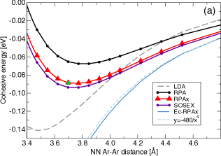
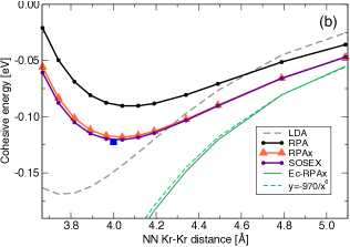
Figure 2: Cohesive energy (eV) as a function of nearest neighbour distance (Å) in solid Ar (a) and Kr (b). The correlation energy (Ec-RPAx) is also shown, together with a fitted $y=k/x^{6}$ curve. Green and blue squares correspond to CCSD(T) results Rościszewski et al. (1999).

Equations (5)-(10) have been implemented within the plane-wave and pseudopotential framework, but have so far only been applied to molecular systems Colonna et al. (2014, 2016); Hellgren et al. (2018). Binding energies have been shown to converge quickly with respect to the number of eigenvalues ($\approx 10$ times the number of electrons ($N_{e}$)). Due to the additional $k$-point sum in $R_{V}$, RPAx scales as $N_{k}^{3}$ with respect to the number of k-points, which can be compared to $N_{k}^{2}$ with RPA. On the other hand, as we will see later, the RPAx converges, in many cases, faster than RPA with respect to $N_{\nu}$.

The underlying many-body formulation of the $f_{\rm x}$-kernel allows also a variant of SOSEX Freeman (1977); Grüneis et al. (2009); Jansen et al. (2010); Ren et al. (2013) to be generated within the present formalism, making use of an alternative resummation of Dyson’s equation (Eq. (3)), that only includes a subset of terms Hellgren et al. (2018). In the following we will present both RPAx and SOSEX results.

Since a fully self-consistent implementation is still not developed, all calculations are done on top of a PBE ground-state Perdew et al. (1997), unless otherwise stated. The electron-ion interaction is treated with standard norm-conserving pseudopotentials Hamann (2013); Goedecker et al. (1996); Schlipf and Gygi (2015).

III Noble gas solids

The ACFD formula for the correlation energy provides a natural starting-point for including the long-range vdW force, i.e., the attractive force between two charge neutral, closed-shell atoms $A$ and $B$ due to fluctuating dipoles present in a correlated wave function. At large separation $R$, the interaction energy can, to leading order, be written as Zaremba and Kohn (1976)

$$E^{AB}=-\frac{1}{R^{6}}\frac{3}{\pi}\int_{0}^{\infty}\!d\omega\,\alpha_{\rm iso}^{A}(i\omega)\alpha_{\rm iso}^{B}(i\omega)\equiv-\frac{C_{6}}{R^{6}},$$ (11)

where

$$\alpha_{\rm iso}^{A}(i\omega)=-\frac{1}{3}\sum_{i}\int\!d^{3}{\bf r}d^{3}{\bf r^{\prime}}x_{i}\,\chi^{A}({\bf r},{\bf r^{\prime}},i\omega)x^{\prime}_{i}$$ (12)

is the isotropic dynamical polarizability of atom $A$, and $C_{6}$ is the vdW coefficient. In Ref. Dobson, 1994, Dobson showed that the RPA correlation energy exactly reproduces Eq. (11), but with the exact polarizability replaced by the RPA polarizability. However, as shown in several previous works, the RPA $C_{6}$-coefficients are underestimated (up to 40% in highly polarizable atoms) Hellgren and von Barth (2010); Toulouse et al. (2010); Gould (2012); Olsen and Thygesen (2013); Toulouse et al. (2013); Ren et al. (2013). For noble gas atoms the error lies at about 17%, which induces an error of approximately 30% in the binding energy of dimers Toulouse et al. (2010); Colonna et al. (2016). Thus, while the RPA captures the vdW forces in a qualitatively correct way, the quantitative errors are large.

Including the xc kernel, it is not straightforward to derive an expression similar to Eq. 11. In fact, in Ref. Gould et al. (2017) it was shown that semilocal kernels produce an additional $1/R^{6}$-term. It remains to be proven analytically whether the nonlocal RPAx reduces to Eq. 11.

In Fig. 2 we have plotted the cohesive energy of solid Ar and Kr as a function of nearest neighbour (NN) distance. In RPA and RPAx a reduced $3\times 3\times 3$ shifted $k$-point grid is used for the correlation energy giving results within 4 meV of the fully converged values (see Appendix C).

In the RPA, the cohesive energy is underestimated by 25%. Our results thus differ somewhat from those obtained in Ref. Harl and Kresse (2008), but are more consistent with the results found for dimers (see Refs. Toulouse et al. (2010); Colonna et al. (2016)). As expected, based on the accurate $C_{6}$-coefficients and dimer binding energies, we find RPAx to be in good agreement with both CCSD(T) Rościszewski et al. (1999) and experimental results Schwalbe et al. (1977). SOSEX gives only slightly larger binding energies.

In Fig. 2 we also display the correlation energy (E_c-RPAx) as a function of NN distance, exhibiting a perfect $1/R^{6}$ behaviour. Given that Ar and Kr have 12 NN the fitted coefficients 67*12 and 135*12 (atomic units) compare well with the dimer $C_{6}$-coefficients of 64 and 130, respectively. Similar accuracy for the $C_{6}$-coefficients are found with other variants of RPAx Toulouse et al. (2013); Ren et al. (2013); Gould and Bucko (2016); Hesselmann (2017) and the renormalized LDA kernel Olsen and Thygesen (2013). We note that the SOSEX defined in Ref. Ren et al. (2013) is different from the one defined here since it does not contain self-energy corrections (here included via $R_{\Sigma}$ in Eq. (4) Hellgren et al. (2018)). The self-energy corrections are similar to the ’single excitations’ in Ref. Ren et al. (2013).

IV Boron nitride and silica

Having established that vdW bonded solids are accurately reproduced with RPAx we now turn to systems were both vdW forces and covalent/ionic bonding are important. The polymorphs of BN consist of the high-pressure cubic (c) and wurtzite (w) structures with fourfold coordinated B/N atoms, and several low-pressure layered structures, such as hexagonal (h) and rhombohedral (r) BN, which are threefold coordinated (see Fig. 3). The density, symmetry and ionic character of the B-N bond change from one phase to the other, with the largest difference between fourfold and threefold coordinated crystals. In these cases, functionals that largely rely on error cancellation become unreliable, producing substantial errors in energy differences that can invert the stability order. Although it is well known that the layered polymorphs need a good description of the vdW forces Marini et al. (2006), this is not the only missing component. Inaccuracies in describing the covalent bond will show up if errors fail to cancel.

In Fig. 4 we plot the interlayer binding energy of r-BN as a function of interlayer distance, keeping the intralayer B-N distance fixed to the experimental value. In general, the interlayer bonding is difficult to model with vdW corrected DFT. Binding energies are typically largely overestimated, often twice as large as RPA values Björkman et al. (2012); Björkman (2014). On the other hand, RPA underestimates the vdW forces, but it is not clear to what extent in layered materials. We have verified that we obtain the same RPA result as in Ref. Björkman et al. (2012), taking into account that h-BN is 5 meV lower in energy than r-BN Cazorla and Gould (2019). The RPAx increases the binding energy by 7 meV (or 9%). This correction is smaller than the correction in purely vdW bonded solids such as Ar and Kr analyzed above. The RPA thus performs better than expected, at least for the BN layered system. We note that, except for some differences in the dissociation tail, the SOSEX and RPAx give essentially the same result.

In the lower panel of Fig. 5 we present results for the energy difference between c-BN and w-BN, and between c-BN and r-BN. c-BN is the reference level at zero in the figure. Calculations are done on experimental structures Paszkowicz et al. (2002). We compare our RPA and RPAx results to recent CCSD and CCSD(T) results Gruber and Grüneis (2018), to LDA and PBE0 (i.e. a hybrid functional with 25% of Fock exchange). We see a striking difference in the performance on the different polymorphs. Both the wurtzite and cubic structures are high-pressure phases with the same B-N coordination and similar volume. This is thus the ideal situation for approximations to benefit from error cancellation. Indeed, almost all approximations give the same value within a couple of meV.

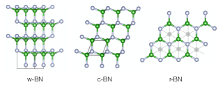
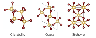
Figure 3: Upper row: wurtzite (w-BN), cubic (c-BN) and layered rhombohedral (r-BN) boron nitride. Lower row: cristobalite and $\alpha$-quartz with fourfold coordinated silicon, and stishovite with sixfold coordinated silicon. Silicon in gold and oxygen in red.

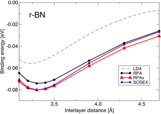
Figure 4: Interlayer binding energy (eV) of r-BN as a function of interlayer separation (Å).

The situation is very different when looking at the r-BN and c-BN energy difference. Here, the volume differ by 35% and the B-N bond change character. LDA is seen to hugely overestimate the energy difference (105 meV) and to predict c-BN to be lowest in energy. Experimental results are mixed but CC results revert the energy order (see Ref. Gruber and Grüneis (2018) and experimental references therein Solozhenko (1991); Fukunaga (2000)). Additionally, PBE0 favours this energy order, predicting r-BN to be lowest in energy, although with a too large energy difference (-67 meV). The RPA, that is known to rely on error cancellation, predicts the same energy order as LDA, but with a smaller energy difference (25 meV). We note that our result is in good agreement with the RPA calculation in Ref. Cazorla and Gould (2019). The RPAx, known to give accurate absolute energies, and not only energy differences, gives a result very close to the CCSD result with an energy difference of -15 meV, and thus reverts the stability order. SOSEX gives a slightly larger energy difference (-23 meV). In Ref. Sengupta et al. (2018) it was shown that the renormalized PBE kernel also provides an improvement upon RPA (-48-(-38) meV). We note that the SOSEX defined here is different from the ACSOSEX defined in Refs. Bates et al. (2016); Sengupta et al. (2018). The latter is based on the renormalized PBE kernel whereas the one here is based on many-body perturbation theory Hellgren et al. (2018).

The difference between RPA and RPAx cannot solely be explained by the difference in how they describe the vdW forces. This suggests that the RPAx captures the covalent B-N bond better than RPA. Our result provides further confirmation that the correct order places the layered low-density structures at a slightly lower energy than the cubic form, even at zero temperature. The difference in zero-point (vibrational) energy (ZPE), has been estimated to -10 meV Cazorla and Gould (2019). We also mention that we tried various DFT functionals employing a vdW correction, again with very mixed results.

In the upper panel of Fig. 5 we show the convergence of the correlation energy difference between c-BN and r-BN ($\Delta E_{\rm c}^{\rm r-c}$) with respect to $N_{\nu}/N_{e}$. We note that when comparing the correlation energy of two systems the same number of eigenvalues per electron has to be used Hellgren et al. (2018). Since r-BN and c-BN have the same number of electrons in the unit cell this implies the same number of eigenvalues. w-BN has twice the number of electrons and, therefore, needs twice the number of eigenvalues. However, while the correlation energy difference between w-BN and c-BN converges quickly with respect to the number of eigenvalues ($<10\times N_{e}$) the RPA exhibits a slow convergence for the r-BN-c-BN energy difference. We used up to 512 eigenvalues in order to produce results within 2 meV (marked by the dashed horizontal lines in Fig. 5), which is more than 60 times the number of electrons and hence 6 times more than usual. The problem of not cancelling errors is thus visible also in this technical aspect of our approach. The absence of this problem is remarkably evident in the convergence of the RPAx correlation energy difference. In RPAx we needed $<64$ eigenvalues, which is similar to the number used for other systems. Further convergence studies can be found in Appendix B.

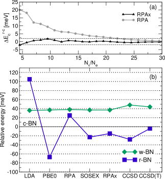
Figure 5: (a) Correlation energy difference of r-BN and c-BN as a function of eigenvalues per electron within RPA and RPAx. (b) Relative energies (meV) of w-BN and r-BN with respect to c-BN within LDA, PBE0, RPA, SOSEX and RPAx. CC results are from Ref. Gruber and Grüneis, 2018. c-BN is the reference value at zero.

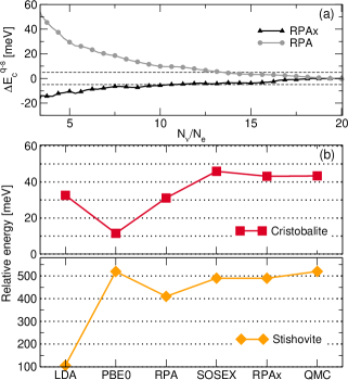
Figure 6: (a) Correlation energy difference of stishovite and $\alpha$-quartz as a function of eigenvalues per electron within RPA and RPAx. (b) Relative energies (meV) between cristobalite and $\alpha$-quartz (red) and between stishovite and $\alpha$-quartz (yellow) within LDA, PBE0, RPA, SOSEX and RPAx. QMC results are from Refs. Driver et al., 2010; Hay et al., 2015.

A similar effect, as studied above in BN, has previously been observed in silica (SiO₂) polymorphs Xiao et al. (2012); Hay et al. (2015); Sengupta et al. (2018). Silica, similar to BN, has polar covalent bonds and polymorphs of different coordination number. In $\alpha$-quartz (space group P3₁21), the most stable crystal at ambient pressure, silicon is fourfold coordinated by oxygen, forming a tetrahedral unit. These units are connected via a flexible Si-O-Si bond, sensitive to vdW forces (see Fig. 3). Cristobalite (space group P4₁2₁2) has a similar local structure and only 5% larger volume. The energy difference between $\alpha$-quartz and cristobalite is found to be approximately 20 meV in experiment Richet et al. (1982); Piccione et al. (2000). When the ZPE contribution is subtracted the energy difference doubles Hay et al. (2015). While LDA predicts the correct energy order PBE erroneously predicts cristobalite to be lower in energy due to missing vdW forces Hay et al. (2015). A similar effect was recently observed in the borate (B₂O₃) polymorphs Ferlat et al. (2019). Stishovite (space group P4₂/mnm) is a high-pressure phase with 37% higher density, having sixfold coordinated Si atoms. The energy difference between stishovite and $\alpha$-quartz is experimentally determined to 0.51-0.54 eV (see Ref. Hamann (1996) and experimental references therein Holm et al. (1967); Akaogi and Navrotsky (1984)). LDA underestimates this value by more than 0.4 eV, whereas PBE here predicts the correct energy difference Hamann (1996).

In the lower panels of Fig. 6 we illustrate the results for the $\alpha$-quartz-cristobalite (red) and $\alpha$-quartz-stishovite (yellow) energy differences. We optimized all structures with PBE plus a vdW correction at the Tkatchenko-Scheffler (TS) level Tkatchenko and Scheffler (2009). In the case of $\alpha$-quartz-cristobalite, LDA gives a value of 33 meV and PBE0 a value of 12 meV. As discussed in Ref. Hay et al. (2015) a vdW correction improves this result. RPA gives a value of 31 meV, which is underestimated by 15 meV according to QMC calculations. As the Si-O bond remains similar in $\alpha$-quartz and cristobalite, we interpret this relatively small error coming from the underestimated vdW forces with RPA. RPAx and SOSEX bring the result in good agreement with the QMC value of 43 meV.

The situation is different in the case of stishovite which has sixfold coordinated Si atoms. Here the variations between the different methods are an order of magnitude larger. Subtracting the ZPE, calculated in Ref. Hay et al. (2015), QMC predicts an energy difference of 0.51 eV Driver et al. (2010), similar to the PBE0 result (0.52 eV) and experiment. With RPAx we find a value of 0.49 eV which is 80 meV larger than the RPA result (0.41 eV). Although still somewhat underestimated we see that the exchange kernel is responsible for the improved accuracy. Self-consistency could further improve this result. That an xc kernel can improve the $\alpha$-quartz-stishovite energy difference was also found in Ref. Sengupta et al. (2018) using the renormalized PBE kernel (0.51-0.54 eV).

Our RPA result differs from the result presented in Ref. Xiao et al. (2012) by 20 meV. The origin of this difference, occurring already at the PBE level, can be traced to the use of PAW (projected augmented wave) potentials Garrity et al. (2014) in Ref. Xiao et al. (2012). A larger difference can be found with respect to the RPA result presented in Ref. Sengupta et al. (2018), a difference that can be traced mainly to the EXX part of the energy (see Appendix C).

From the technical point of view the situation is similar to the BN polymorphs. In the upper panel of Fig. 6 we show the convergence of the $\alpha$-quartz-stishovite correlation energy difference ($\Delta E_{\rm c}^{\rm q-s}$) with respect to $N_{\nu}$. Again, we find a slower convergence in RPA as compared to RPAx. The RPA and RPAx values were converged within 10 meV using $30\times N_{e}$ and $10\times N_{e}$ eigenvalues, respectively.

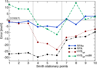
Figure 7: Error in the binding energy (meV) with respect to CCSD(T) for the 10 Smith stationary points.

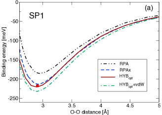
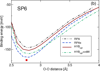
Figure 8: Binding energy (meV) as a function of O-O distance (Å) of water dimers in the SP1 (a) and SP6 (b) configuration. Red square corresponds to the CCSD(T) result Tschumper et al. (2002).

V Ice polymorphism

The problem in predicting the relative energies between high- and low-pressure phases is relevant also for molecular solids such as the ice polymorphs. At ambient pressure the oxygen atoms in water form an hexagonal lattice held together by hydrogen bonds. By applying pressure the average O-O distance reduces such that the oxygen atoms are approached in non-hydrogen bonded configurations, which increases the coordination number from four up to eight in some dense high-pressure structures Gillan et al. (2016).

Table 1: Anisotropic polarizability (a.u.) of the water molecule. In the first two columns results are obtained with PBE orbitals and in the second two columns with the optimized hybrid orbitals (20% of exchange for RPA and 35% for RPAx). Geometry and CC results are from Refs. Elking et al., 2011; Loboda et al., 2016.

	RPA	RPAx	RPA	RPAx	CCSD	CCSD(T)
	PBE orbitals		HYBopt orbitals
$\alpha_{xx}$	9.14	9.66	8.49	8.76	8.976	9.250
$\alpha_{yy}$	9.19	10.35	8.78	9.69	9.712	9.874
$\alpha_{zz}$	9.19	9.87	8.66	9.18	9.310	9.529
$\alpha_{\rm iso}$	9.17	9.96	8.64	9.21	9.33	9.55
MAE	-0.38	+0.41	-0.91	-0.35	-0.22

Calculating the energy difference between these phases with standard functionals in DFT, again produces large errors. One of the failures has been attributed to the lack of vdW forces, which are expected to play an important role in high-pressure phases as well as liquid water Lin et al. (2009); Jonchiere et al. (2011); Santra et al. (2011, 2013). In addition, a fraction of HF exchange has shown to be important for the description of the hydrogen bond Santra et al. (2011, 2013). However, combining a hybrid functional with a vdW correction still does not give a complete description. The strongly constrained and appropriately normed (SCAN) meta-GGA functional Sun et al. (2015) has shown that it is possible to obtain good energy differences between low- and high-density phases using a semi-local functional. On the other hand, lattice energies, i.e., the energy gain per monomer in the solid, remain overestimated with SCAN Sun et al. (2016). The more advanced RPA also provides improved energy differences, but in this case with underestimated lattice energies Macher et al. (2014), due to the poor description of the hydrogen bond within RPA Zhu et al. (2010); Dixit et al. (2017); Hellgren et al. (2018). Calculations using second order Møller-Plesset perturbation theory have, indeed, shown that higher order exchange terms are important Gillan et al. (2013).

We will now investigate the performance of the RPAx, and start by exposing a fundamental problem of the RPA when calculating the polarizability of the water molecule. Since the static polarizability $\alpha(0)$ (Eq. (12)) is not a variational quantity like the total energy, it has a stronger dependency on the input orbitals (and eigenvalues) van Gisbergen et al. (1998). It can be argued that the correct orbitals should be those coming from a self-consistent RPA/RPAx calculation Hellgren and von Barth (2010). However, instead of these orbitals, we will use both PBE orbitals and orbitals from an optimal hybrid functional based on a local KS potential Hellgren et al. (2021). The optimization of the hybrid functional is carried out by minimizing the total RPA/RPAx energy with respect to the fraction of exact-exchange in hybrid functional used to generate the input orbitals (see further details in Appendix A and Ref. Nguyen et al. (2014)). In order to study effects of anisotropy we calculate all diagonal elements of the polarizability. The results, obtained using the geometry of Refs. Elking et al., 2011; Loboda et al., 2016, are presented in Table I. We see that RPA clearly underestimates the polarizability and the magnitude of anisotropy when evaluated with optimal hybrid orbitals (20% of exchange in RPA). The isotropic RPA polarizability improves with PBE orbitals, but the anisotropy is then completely lost. The origin of any anisotropy within RPA is, thus, solely due to an effect of exchange in the description of the orbitals. In contrast, the RPAx exhibits anisotropy already with PBE orbitals stemming from the exchange kernel. This effect is enhanced using optimal hybrid orbitals (35% of exchange in RPAx). The RPAx agrees very well with CCSD results Elking et al. (2011), and are not so far from CCSD(T) results Loboda et al. (2016). These results highlight the important role of the exchange kernel for describing not only the water molecule, but also the long-range interaction between water molecules.

In order to study the water intermolecular interaction in more detail we determine the binding energy of the ten Smith stationary points (SPs) Smith et al. (1990). In addition to the global minimum, the SPs correspond to transition states or higher order saddle points on the water dimer potential energy surface Tschumper et al. (2002). The geometries of the SPs, depicted Appendix C are relevant for liquid water Santra et al. (2009); Gillan et al. (2012), and some are found in high-pressure ice polymorphs. The lowest energy configuration (SP1) corresponds to the optimal hydrogen bond geometry, included in many molecular test-sets. Previous work has shown that RPAx and related methods capture the binding energy of this configuration rather well, while RPA fails by around 15% Zhu et al. (2010); Dixit et al. (2017); Hellgren et al. (2018). In Fig. 7 we have summarized the results for all ten SPs using structures optimized at the CCSD(T) level Tschumper et al. (2002). The HYB_opt corresponds to the hybrid functional optimised with RPAx (35% of exchange). The HYB_opt orbitals were used for evaluating the energy in both RPA and RPAx. For the total energy the choice of orbitals has a small effect. The largest difference is found for the SP1 configuration where the RPAx binding energy change from 212 meV to 216 meV when going from PBE to HYB_opt orbitals. We have also included a vdW correction at the TS level in combination with the same hybrid (HYB_opt+vdW). Errors are determined with respect CCSD(T) reference values Tschumper et al. (2002). It is clear that RPA fails not only for SP1 but for all configurations. The error is, however, rather constant suggesting that the energy differences are still quite well described. The hybrid functional performs very well for the first three hydrogen bonded configurations but fails, similarly to RPA, for the others. Energy differences will, in this case, not benefit from error cancellation. Adding the TS-vdW correction shifts all values with a similar constant (except for SP8). The vdW correction thus improves results for some configurations and worsens the results for others, but the quality of the energy difference will be similar to that of the hybrid functional without a vdW correction. These results show how complex and challenging it is to capture the full (H₂O)₂ potential energy surface. RPAx is the only approximation that performs well for all SPs and produces results comparable to reference values at the CCSD(T) level.

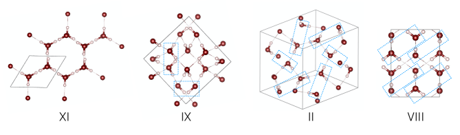
Figure 9: Structures of the four ice polymorphs studied in this work (XI, IX, II, VIII). Blue dashed boxes indicate water dimers in non-hydrogen bonded configurations but with comparable O-O distance.

In Fig. 8 we plot the dissociation energy curves of the SP1 and SP6 configurations. The dimers are stretched with fixed intramolecular geometries. Given the accuracy of the RPAx we can now use this approximation as a reference to compare the other methods too. It is interesting to note that the hybrid functional which gives a good value at the SP1 bond midpoint also captures the dissociation tail. RPAx and HYB_opt perfectly coincides up to 5 Å. Adding a vdW correction improves the binding energy of the SP6 configuration. However, from the full dissociation curve, we see that this is at the expense of producing the wrong tail. Even in this non-hydrogen bonded configuration, RPAx and HYB_opt are closer at stretched geometries.

We are now ready to study solid forms of water. In Fig. 9 we illustrate four different phases of ice in the order of decreasing volume per molecular unit: XI, II, IX and VIII. All structures are relaxed with the PBE+TS functional. Due to the smaller unit cell, we have chosen the ferroelectrically proton-ordered ice XI (Cmc2₁) instead of the ordinary disordered I_h Tajima et al. (1982); Hirsch and Ojamae (2004). The energy of XI is three meV lower than I_h in RPA Macher et al. (2014). Both are purely hydrogen bonded solids with water molecules arranged in SP(1-3)-like configurations. In clusters and solids the strength of the hydrogen bond is enhanced as compared to the isolated dimer bond strength. This effect is captured by most functionals. In Table II we present lattice energies using HYB_opt, HYB_opt+vdW, RPA, RPAx and SOSEX. The results are compared to CCSD(T) Gillan et al. (2013) and recent QMC results Zen et al. (2018). We see that both HYB_opt and RPAx produce a result for XI of similar quality as for the SP1 dimer. In the same way, RPA underestimates the lattice energy. We note that for the solids we have evaluated both RPA and RPAx with PBE orbitals in order to compare with previous RPA results Macher et al. (2014). The use of HYB_opt orbitals (always via a local potential) increases the XI result by 10 meV ($<2\%$).

Table 2: Lattice energies (meV) of ice XI, II, IX and VIII with the optimized hybrid functional HYB_opt (35% exchange), the same hybrid functional with a TS-vdW correction, RPA, RPAx, SOSEX, CCSD(T) Gillan et al. (2013), QMC Zen et al. (2018) and experiment Whalley (1984). The relative energies with respect to XI are also presented. For CCSD(T) and QMC XI should be replaced by I_h.

Ice	HYBopt	HYBopt+vdW	RPA	RPAx	SOSEX	CCSD(T)	QMC	Exp.
XI (Cmc21)	614	676	551	609	634	601	615	610
II	559	671	542	609	639	601	613	609
IX	570	673	538	598	625	-	-	606
VIII	471	606	516	584	613	574	594	595
II—XI	55	5	9	0	-5	0	2	1
IX—XI	44	3	13	11	9	-	-	4
VIII—XI	143	70	35	25	21	27	21	15

Ice IX and II have similar volumes, approximately 20% smaller than XI. The smaller volume makes non-hydrogen bonded configurations more relevant. In Fig. 9 we have identified pairs of H₂O monomers for which the magnitude of the O-O distance is approaching that of hydrogen-bonded configurations. The ability of a functional to capture the energies of different dimer orientations thus increases in importance for the IX and II phases. In Table II we see that the good performance of HYB_opt is now lost, producing underestimated lattice energies. Adding the vdW correction overcorrects the lattice energies but recovers the near degeneracies between XI, II and IX. This result was highlighted in Ref. Santra et al. (2011) suggesting that the vdW forces play an important role in the II and IX phases. We note that the most recent QMC calculation predicts ice II and I_h to be nearly degenerate at 613 and 615 meV, respectively (with a 5 meV error bar) Zen et al. (2018), while an earlier QMC calculation from 2011 predicts ice II to be lower in energy than I_h by 4 meV (609 and 605 meV respectively) Santra et al. (2011). The corresponding experimental results have been extracted in Ref. Whalley (1984), yielding 609 and 610 meV respectively. Our RPA calculation gives an II-XI energy difference of 9 meV, in good agreement with previous calculations Macher et al. (2014). RPAx clearly reduces this energy difference making them degenerate. SOSEX lowers the energy of ice II with respect XI even further, reverting the energy order. Given that ice XI is expected to be a couple of meV lower in energy than I_h, even by experiment Leadbetter et al. (1985), our results indicate that the II-I_h energy difference should be $\leq$ 0 meV. We also note that HYB_opt and HYB_opt+vdW predict ice IX to be lower in energy than ice II, in contrast to the present (beyond-)RPA methods and the previously mentioned SCAN functional Sun et al. (2016).

Ice VIII has a volume 40% smaller than ice IX and is stable above 2 GPa. It corresponds to a proton-ordered phase of VII Pruzan et al. (1993); Song et al. (2003). In this structure the O atoms are eightfold coordinated and it is easy to identify both SP6-like and SP8-like dimers, in addition to the hydrogen bonded configurations. As pointed out in Ref. Gillan et al. (2016) the smallest O-O distance is actually between monomers in non-hydrogen bonded configurations. The experimental result for the lattice energy was initially determined to 577 meV Whalley (1984). Later, this has been revised to 595 meV Zen et al. (2018). Again HYB_opt fails, while HYB_opt+vdW only slightly overcorrects in this case. The energy difference with respect to ice XI remains, however, largely overestimated. The error of the RPA is slightly larger than for the other polymorphs. RPAx is again very accurate lying between CCSD(T) and QMC.

Overall the RPA results for the ice polymorphs are consistent with the analysis of the SPs above. Lattice energies are underestimated by approximately 13%, which is very similar to the error found for the SPs. Relative energies are much better described, benefiting from error cancellation. RPAx, which captures the essential correlation effects, gets both lattice energies and relative energies in good agreement with experiment and more sophisticated methods. SOSEX slightly overestimates the hydrogen bond and thereby overestimates the lattice energies for all polymorphs.

VI Conclusions

The RPA is becoming an important tool in materials science for calculating ground-state properties of solids. There are, however, some inherent limitations of the RPA which can cause significant errors in certain systems or situations. In this work we have analyzed some of these cases and demonstrated how exact-exchange in the response function provides a theoretically well-defined, accurate and reliable improvement.

In general, the exchange term increases atomic polarizabilities leading to, e.g., improved vdW coefficients. Here we have shown that for the cohesive energy of purely vdW bonded solids, such as Ar and Kr, RPAx produces very accurate results, improving the RPA by more than 20%. vdW forces also play an important role in the SiO₂ and BN polymorphs. We have shown that the interlayer binding energy of r-BN is enhanced with RPAx. However, with a smaller correction than for purely vdW bonded systems. The $\alpha$-quartz-cristobalite energy difference is also enhanced with RPAx, and now agrees with reference QMC calculations.

Earlier work have shown that the RPAx corrects the overestimated RPA correlation energy. As often pointed out, this error cancels to a large extent when looking at energy differences of similar systems. Which systems are similar enough is, however, not well-defined. In this work we have highlighted that when the coordination number changes, as between high- and low-pressure phases, errors do not cancel to a satisfactory degree. This has been demonstrated for the r-BN-c-BN and the $\alpha$-quartz-stishovite energy differences. In the first case, RPA and RPAx predict different energy ordering, and in the second case, RPAx strongly enhances the energy difference. In both cases RPAx produces results in line with highly accurate methods such as CC or QMC.

We have also studied the (H₂O)₂ potential energy surface and ice polymorphism. The errors of RPA (and hybrid functionals) in describing the lattice energies of ice IX, II, XI and VIII were analysed in terms of the polarizability of the water molecule and the 10 SPs. The RPA clearly underestimates both magnitude and anisotropy of the polarizability, but captures rather well the energy differences between different H₂O dimer configurations thanks to a good error cancellation. This implies underestimated lattice energies of ice but good relative energies. The RPAx, which includes higher order exchange effects, captures the correct strength of the hydrogen bond and is able to describe the full anisotropic interaction between H₂O monomers. Not only relative energies but also lattice energies are, thereby, in very good agreement with experiment and more sophisticated methods.

Regarding the computational cost and feasibility of the RPAx the main constraint is the $N^{3}_{k}$ scaling, which can make k-point demanding systems several times more expensive than RPA. On the other hand, the convergence with respect to eigenvalues in the response function is in many cases faster with RPAx. Other parameters such as the total number of k-points or frequency points have a similar behaviour in RPA and RPAx. For the systems studied here, the cost of the RPAx calculation is 3-10 times that of the RPA calculation.

All calculations were done non-self-consistently, on top of a PBE ground-state. For the water dimers and ice we showed that the use of hybrid orbitals, which can be considered as a step towards self-consistency, increases the energy differences by a few meV only. Further developments in this direction are, however, interesting for eventually calculating forces and lattice vibrations within the same framework.

To conclude, we have shown that the RPAx opens up for highly accurate density functional calculations on solids that can address structural phase transitions involving distinct but nearly degenerate phases, and provide more reliable reference results than RPA when experimental data are missing or difficult to access.

Appendix A Exchange parameter for water

The polarizability is more sensitive to the choice of input orbitals than the total energy. In Ref. Hellgren and von Barth (2010) the atomic polarizabilites were evaluated with self-consistent RPA/RPAx orbitals. Since self-consistent RPA/RPAx is not yet available for molecules we have, in this work, evaluated the polarizability with PBE orbitals and orbitals coming from PBE0 hybrid functional, in which the $\alpha$-parameter was optimized by minimizing the total RPA/RPAx energy (see Fig. 10).

The local xc potential of the hybrid functional is defined as the functional derivative of the hybrid xc energy with respect to the density. It can thus be decomposed into

$$v_{\rm xc}^{\rm hyb,\alpha}=v^{\alpha}_{{\rm x}}+(1-\alpha)v^{\rm PBE}_{{\rm x}}+v^{\rm PBE}_{\rm c}.$$ (13)

For the exchange part, an integral equation known as the linearized Sham-Schlüter equation has to be solved

$$\int\!d2\,\chi_{s}(1,2)v^{\alpha}_{{\rm x}}(2)=\alpha\int\!d2d3\,\Lambda_{s}(3,2;1)\Sigma_{s}^{\rm HF}(2,3)$$ (14)

where $\Sigma_{s}^{\rm HF}(2,3)$ is the Fock self-energy, $\Lambda_{s}(3,2;1)=-iG_{s}(3,1)G_{s}(1,2)$ is the product of two Kohn-Sham Green’s functions, $G_{s}$, and $\chi_{s}=\Lambda_{s}(2,2;1)$. Details of the implementation can be found in Refs. Nguyen et al. (2014); Hellgren et al. (2021)

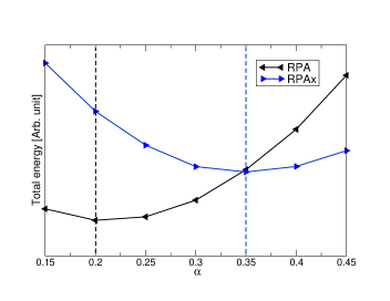
Figure 10: The $\alpha$-parameter of the hybrid functional was chosen so as to minimize the total energy of the water molecule. The minimum occurs at 20% in RPA and at 35% in RPAx.

Appendix B Convergence of $N_{\nu}$ and $N_{k}$

We include here additional results for the convergence of crucial parameters such as the number of eigenvalues in the response function ($N_{\nu}$), and the number of k-points ($N_{k}$). We used an energy cut-off of 80 Ry in all calculations except for the SiO₂ polymorphs where we converged the correlation energy with 60 Ry.

The convergence with respect to $N_{\nu}$ for the $\alpha$-quartz-stishovite and c-BN-r-BN energy difference is presented in the main text. Here, in Fig. 11, we present the $N_{\nu}$-convergence for the cohesive energy of Ar, the interlayer binding energy of r-BN, the $\alpha$-quartz-cristobalite energy difference and the binding energy of the water dimer. For these systems a value $N_{\nu}<10*N_{e}$ is sufficient to converge within 2 meV for both RPA and RPAx.

In Fig. 12 we present the convergence of the correlation energy with respect k-points for Ar, c-BN, stishovite and Ice-XI. We used shifted grids for faster convergence. Ar and Kr were converged within 2 meV using a $5\times 5\times 5$ grid. For c-BN the last point corresponds to a $6\times 6\times 6$ grid. For stishovite the last point corresponds to a $4\times 4\times 4$ grid. In order to save computing hours, the last RPAx point for stishovite is obtained by extrapolation, using the fact that the ratio between the RPA and RPAx correlation energy differences is essentially a constant. The last point for Ice-XI corresponds to a $3\times 3\times 2$ grid.

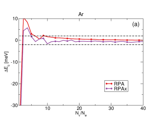
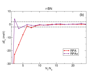
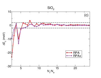
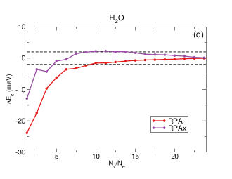
Figure 11: Convergence of the correlation energy difference with respect to the number of eigenvalues per electron in the response function. (a) correlation energy difference between solid Argon and the isolated Ar atom, (b) between layered r-BN and an isolated BN layer, (c) between $\alpha$-quartz and cristobalite and, (d) between the water dimer and an isolated water molecule.

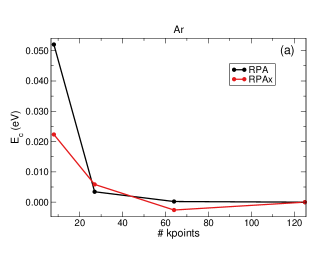
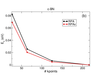
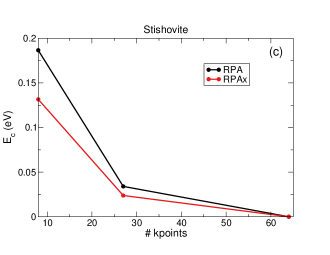
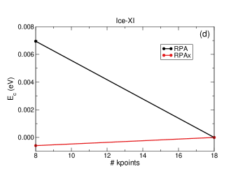
Figure 12: Convergence of the correlation energy of (a) Ar, (b) c-BN, (c) stishovite and (d) Ice-XI with respect to the number of k-points. Curves have been shifted vertically by subtracting the value at the last point.

Appendix C Tables

We have included 6 tables. Table 3 contains the cohesive energy of Ar and Kr, and table 4 the interlayer binding energy of r-BN. Table 5 contains the energy of r-BN and w-BN with respect to c-BN, and table 6 the energy of cristobalite and stishovite with respect to $\alpha$-quartz. Tables 7 and 8 contain the binding- and relative energies of the 10 Smith points (SPs), respectively. An illustration of the 10 SPs can be found in Fig. 13.

Table 3: Cohesive energies of Ar and Kr (meV) in LDA, EXX, RPA, RPAx, SOSEX, CCSD(T) Rościszewski et al. (1999) and experiment Schwalbe et al. (1977).

Solid	LDA	EXX	RPA	RPAx	SOSEX	CCSD(T)	Exp.
Ar	141	-104	69	86	91	83	89
Kr	169	-102	94	117	120	114	123

Table 4: Interlayer binding energy of r-BN (meV) in LDA, EXX, RPA, RPAx and SOSEX. No accurate reference value is available.

Solid	LDA	EXX	RPA	RPAx	SOSEX
r-BN	56	-58	74	80	80

Table 5: Energy difference with respect to c-BN (meV) in LDA, PBE0, EXX, RPA, RPAx, SOSEX, CCSD Gruber and Grüneis (2018) and CCSD(T) Gruber and Grüneis (2018).

Solid	LDA	PBE0	EXX	RPA	RPAx	SOSEX	CCSD	CCSD(T)
r-BN	105	-67	-442	25	-15	-23	-28	-4
w-BN	36	37	48	38	37	37	48	44

Table 6: Energy difference with respect to $\alpha$-quartz in LDA, PBE0, EXX, RPA, RPAx, SOSEX, QMC Driver et al. (2010); Hay et al. (2015) and experiment Richet et al. (1982); Piccione et al. (2000); Holm et al. (1967); Akaogi and Navrotsky (1984).

Solid	LDA	PBE0	EXX	RPA	RPAx	SOSEX	QMC	Exp.
Cristobalite (meV)	32	11	6	31	43	46	43$\pm 8$	46-51
Stishovite (eV)	0.11	0.52	1.33	0.41	0.49	0.49	0.51$\pm 0.02$	0.51-0.54

Table 7: Binding energy of the 10 Smith stationary points with a hybrid functional HYB_opt (35% of exchange), the same hybrid functional with a TS vdW correction, RPA, RPAx, SOSEX and CCSD(T) Tschumper et al. (2002) (meV). Mean absolute (percentual) error is calculated with the CCSD(T) results as reference.

SP	HYBopt	HYBopt+ vdW	RPA	RPAx	SOSEX	CCSD(T)
1	216.8	230.0	190.4	215.9	224.0	217.6
2	193.7	205.5	169.7	194.5	202.2	195.6
3	189.9	201.3	166.3	191.7	199.5	192.6
4	169.8	184.1	157.9	182.1	190.4	187.6
5	157.6	169.3	149.0	171.7	178.5	176.6
6	149.9	162.0	145.3	167.8	173.6	174.6
7	124.6	138.9	122.4	139.5	144.0	138.6
8	50.7	77.2	49.8	60.0	62.8	63.6
9	131.5	141.1	127.3	143.6	147.4	140.6
10	93.2	103.2	91.0	103.6	106.3	100.6
MAE	11.0	6.9	21.9	3.1	4.2	-
MA%E	8.1	5.2	14.0	2.3	2.8	-

Table 8: Relative energies of 10 Smith stationary points with respect to SP1 using the hybrid functional HYB_opt (35% of exchange), the same hybrid functional with a TS vdW correction, RPA, RPAx, SOSEX and CCSD(T) Tschumper et al. (2002) (meV). Mean absolute error is calculated with the CCSD(T) results as reference.

SP	HYBopt	HYBopt+ vdW	RPA	RPAx	SOSEX	CCSD(T)
1	0	0	0	0	0	0
2	23.1	24.5	20.7	21.4	21.8	22
3	26.9	28.7	24.1	24.2	24.4	25
4	47.0	45.9	32.4	33.9	33.6	30
5	59.2	60.7	41.4	44.2	45.4	41
6	66.9	68.0	45.1	48.2	50.4	43
7	92.2	91.1	68.0	76.4	80.0	78
8	166.1	152.8	140.6	155.9	161.2	154
9	85.3	88.9	63.1	72.4	76.6	77
10	123.6	126.8	99.4	112.4	117.7	117
MAE	11.4	11.3	6.8	2.9	2.8	-

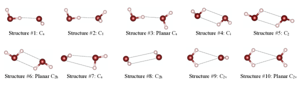
Figure 13: Illustration of the 10 Smith stationary points of the (H₂O)₂ potential energy surface.

References

- Hohenberg and Kohn (1964) P. Hohenberg and W. Kohn, “Inhomogeneous electron gas,” Phys. Rev. 136, B864–B871 (1964).
- Kohn and Sham (1965) W. Kohn and L. J. Sham, “Self-consistent equations including exchange and correlation effects,” Phys. Rev. 140, A1133–A1138 (1965).
- Björkman et al. (2012) T. Björkman, A. Gulans, A. V. Krasheninnikov, and R. M. Nieminen, “van der waals bonding in layered compounds from advanced density-functional first-principles calculations,” Phys. Rev. Lett. 108, 235502 (2012).
- Gillan et al. (2016) Michael J. Gillan, Dario Alfè, and Angelos Michaelides, “Perspective: How good is DFT for water?” The Journal of Chemical Physics 144, 130901 (2016).
- Hay et al. (2015) Henri Hay, Guillaume Ferlat, Michele Casula, Ari Paavo Seitsonen, and Francesco Mauri, “Dispersion effects in polymorphs: An ab initio study,” Phys. Rev. B 92, 144111 (2015).
- Nguyen and de Gironcoli (2009) Huy-Viet Nguyen and Stefano de Gironcoli, “Efficient calculation of exact exchange and RPA correlation energies in the adiabatic-connection fluctuation-dissipation theory,” Phys. Rev. B 79, 205114 (2009).
- Harl and Kresse (2009) Judith Harl and Georg Kresse, “Accurate bulk properties from approximate many-body techniques,” Phys. Rev. Lett. 103, 056401 (2009).
- Ren et al. (2012) Xinguo Ren, Patrick Rinke, Christian Joas, and Matthias Scheffler, “Random-phase approximation and its applications in computational chemistry and materials science,” Journal of Materials Science 47, 7447 (2012).
- Langreth and Perdew (1975) D.C. Langreth and J.P. Perdew, “The exchange-correlation energy of a metallic surface,” Solid State Communications 17, 1425 – 1429 (1975).
- Stromsheim et al. (2011) Marie D. Strömsheim, Naveen Kumar, Sonia Coriani, Espen Sagvolden, Andrew M. Teale, and Trygve Helgaker, “Dispersion interactions in density-functional theory: An adiabatic-connection analysis,” The Journal of Chemical Physics 135, 194109 (2011).
- Xiao et al. (2012) Bing Xiao, Jianwei Sun, Adrienn Ruzsinszky, Jing Feng, and John P. Perdew, “Structural phase transitions in Si and SiO2 crystals via the random phase approximation,” Phys. Rev. B 86, 094109 (2012).
- Sengupta et al. (2018) Niladri Sengupta, Jefferson E. Bates, and Adrienn Ruzsinszky, “From semilocal density functionals to random phase approximation renormalized perturbation theory: A methodological assessment of structural phase transitions,” Phys. Rev. B 97, 235136 (2018).
- Zhu et al. (2010) Wuming Zhu, Julien Toulouse, Andreas Savin, and János G. Ángyán, “Range-separated density-functional theory with random phase approximation applied to noncovalent intermolecular interactions,” The Journal of Chemical Physics 132, 244108 (2010).
- Dixit et al. (2017) Anant Dixit, Julien Claudot, Sébastien Lebègue, and Dario Rocca, “Improving the efficiency of beyond-RPA methods within the dielectric matrix formulation: Algorithms and applications to the a24 and s22 test sets,” Journal of Chemical Theory and Computation 13, 5432–5442 (2017).
- Hellgren et al. (2018) Maria Hellgren, Nicola Colonna, and Stefano de Gironcoli, “Beyond the random phase approximation with a local exchange vertex,” Phys. Rev. B 98, 045117 (2018).
- Lein et al. (2000) Manfred Lein, E. K. U. Gross, and John P. Perdew, “Electron correlation energies from scaled exchange-correlation kernels: Importance of spatial versus temporal nonlocality,” Phys. Rev. B 61, 13431–13437 (2000).
- Marques et al. (2006) Miguel Marques, Angel Rubio, E. K. U. Gross, Kieron Burke, Fernando Nogueira, and Carsten A Ullrich, Time-dependent density functional theory, Vol. 706 (Springer, Berlin, Heidelberg, 2006).
- Gross and Kohn (1985) E. K. U. Gross and Walter Kohn, “Local density-functional theory of frequency-dependent linear response,” Phys. Rev. Lett. 55, 2850–2852 (1985).
- van Leeuwen (1998) Robert van Leeuwen, “Causality and symmetry in time-dependent density-functional theory,” Phys. Rev. Lett. 80, 1280–1283 (1998).
- von Barth et al. (2005) Ulf von Barth, Nils Erik Dahlen, Robert van Leeuwen, and Gianluca Stefanucci, “Conserving approximations in time-dependent density functional theory,” Phys. Rev. B 72, 235109 (2005).
- Furche and Van Voorhis (2005) Filipp Furche and Troy Van Voorhis, “Fluctuation-dissipation theorem density-functional theory,” The Journal of Chemical Physics 122, 164106 (2005).
- Olsen and Thygesen (2012) Thomas Olsen and Kristian S. Thygesen, “Extending the random-phase approximation for electronic correlation energies: The renormalized adiabatic local density approximation,” Phys. Rev. B 86, 081103(R) (2012).
- Olsen and Thygesen (2014) Thomas Olsen and Kristian S. Thygesen, “Accurate ground-state energies of solids and molecules from time-dependent density-functional theory,” Phys. Rev. Lett. 112, 203001 (2014).
- Olsen et al. (2019) Thomas Olsen, Christopher E Patrick, Jefferson E Bates, Adrienn Ruzsinszky, and Kristian S Thygesen, “Beyond the RPA and GW methods with adiabatic xc-kernels for accurate ground state and quasiparticle energies,” npj Computational Materials 5, 1–23 (2019).
- Fetter and Walecka (2003) Alexander L. Fetter and John D. Walecka, Quantum Theory of Many-Particle Systems (Dover Publications, 2003).
- Görling (1998) Andreas Görling, “Exact exchange-correlation kernel for dynamic response properties and excitation energies in density-functional theory,” Phys. Rev. A 57, 3433–3436 (1998).
- Hellgren and von Barth (2008) Maria Hellgren and Ulf von Barth, “Linear density response function within the time-dependent exact-exchange approximation,” Phys. Rev. B 78, 115107 (2008).
- Hellgren and von Barth (2010) Maria Hellgren and Ulf von Barth, “Correlation energy functional and potential from time-dependent exact-exchange theory,” The Journal of Chemical Physics 132, 044101 (2010).
- elmann and Görling (2010) Andreas Heßelmann and Andreas Görling, “Random phase approximation correlation energies with exact kohn-sham exchange,” Molecular Physics 108, 359–372 (2010).
- Freeman (1977) David L. Freeman, “Coupled-cluster expansion applied to the electron gas: Inclusion of ring and exchange effects,” Phys. Rev. B 15, 5512–5521 (1977).
- Grüneis et al. (2009) Andreas Grüneis, Martijn Marsman, Judith Harl, Laurids Schimka, and Georg Kresse, “Making the random phase approximation to electronic correlation accurate,” The Journal of Chemical Physics 131, 154115 (2009).
- Jansen et al. (2010) Georg Jansen, Ru-Fen Liu, and János G. Ángyán, “On the equivalence of ring-coupled cluster and adiabatic connection fluctuation-dissipation theorem random phase approximation correlation energy expressions,” The Journal of Chemical Physics 133, 154106 (2010).
- Ren et al. (2013) Xinguo Ren, Patrick Rinke, Gustavo E. Scuseria, and Matthias Scheffler, “Renormalized second-order perturbation theory for the electron correlation energy: Concept, implementation, and benchmarks,” Phys. Rev. B 88, 035120 (2013).
- Colonna et al. (2014) Nicola Colonna, Maria Hellgren, and Stefano de Gironcoli, “Correlation energy within exact-exchange adiabatic connection fluctuation-dissipation theory: Systematic development and simple approximations,” Phys. Rev. B 90, 125150 (2014).
- Colonna et al. (2016) Nicola Colonna, Maria Hellgren, and Stefano de Gironcoli, “Molecular bonding with the RPAx: From weak dispersion forces to strong correlation,” Phys. Rev. B 93, 195108 (2016).
- Bleiziffer et al. (2015) Patrick Bleiziffer, Marcel Krug, and Andreas Görling, “Self-consistent Kohn-Sham method based on the adiabatic-connection fluctuation-dissipation theorem and the exact-exchange kernel,” The Journal of Chemical Physics 142, 244108 (2015).
- Cazorla and Gould (2019) Claudio Cazorla and Tim Gould, “Polymorphism of bulk boron nitride,” Science Advances 5 (2019), 10.1126/sciadv.aau5832.
- Gruber and Grüneis (2018) Thomas Gruber and Andreas Grüneis, “Ab initio calculations of carbon and boron nitride allotropes and their structural phase transitions using periodic coupled cluster theory,” Phys. Rev. B 98, 134108 (2018).
- Marini et al. (2006) Andrea Marini, P. García-González, and Angel Rubio, “First-principles description of correlation effects in layered materials,” Phys. Rev. Lett. 96, 136404 (2006).
- Mussard et al. (2016) Bastien Mussard, Dario Rocca, Georg Jansen, and János G. Ángyán, “Dielectric matrix formulation of correlation energies in the random phase approximation: Inclusion of exchange effects,” Journal of Chemical Theory and Computation 12, 2191–2202 (2016).
- Toulouse et al. (2009) Julien Toulouse, Iann C. Gerber, Georg Jansen, Andreas Savin, and János G. Ángyán, “Adiabatic-connection fluctuation-dissipation density-functional theory based on range separation,” Phys. Rev. Lett. 102, 096404 (2009).
- Rościszewski et al. (1999) Krzysztof Rościszewski, Beate Paulus, Peter Fulde, and Hermann Stoll, “Ab initio calculation of ground-state properties of rare-gas crystals,” Phys. Rev. B 60, 7905–7910 (1999).
- Perdew et al. (1997) John P. Perdew, Kieron Burke, and Matthias Ernzerhof, “Generalized gradient approximation made simple,” Phys. Rev. Lett. 77, 3865 (1997).
- Hamann (2013) D. R. Hamann, “Optimized norm-conserving vanderbilt pseudopotentials,” Phys. Rev. B 88, 085117 (2013).
- Goedecker et al. (1996) S. Goedecker, M. Teter, and J. Hutter, “Separable dual-space gaussian pseudopotentials,” Phys. Rev. B 54, 1703–1710 (1996).
- Schlipf and Gygi (2015) Martin Schlipf and Francois Gygi, “Optimization algorithm for the generation of oncv pseudopotentials,” Computer Physics Communications 196, 36 – 44 (2015).
- Zaremba and Kohn (1976) E. Zaremba and W. Kohn, “Van der waals interaction between an atom and a solid surface,” Phys. Rev. B 13, 2270–2285 (1976).
- Dobson (1994) J.F Dobson, “Topics in condensed matter physics,” (Nova, 1994) Chap. Quasi-local-density approximation for a van der Waals energy functional, p. 121.
- Toulouse et al. (2010) Julien Toulouse, Wuming Zhu, János G. Ángyán, and Andreas Savin, “Range-separated density-functional theory with the random-phase approximation: Detailed formalism and illustrative applications,” Phys. Rev. A 82, 032502 (2010).
- Gould (2012) Tim Gould, “Communication: Beyond the random phase approximation on the cheap: Improved correlation energies with the efficient radial exchange hole kernel,” The Journal of Chemical Physics 137, 111101 (2012).
- Olsen and Thygesen (2013) Thomas Olsen and Kristian S. Thygesen, “Beyond the random phase approximation: Improved description of short-range correlation by a renormalized adiabatic local density approximation,” Phys. Rev. B 88, 115131 (2013).
- Toulouse et al. (2013) Julien Toulouse, Elisa Rebolini, Tim Gould, John F. Dobson, Prasenjit Seal, and János G. Ángyán, “Assessment of range-separated time-dependent density-functional theory for calculating c6 dispersion coefficients,” The Journal of Chemical Physics 138, 194106 (2013).
- Gould et al. (2017) Tim Gould, Julien Toulouse, János G. Ángyán, and John F. Dobson, “Casimir?polder size consistency: A constraint violated by some dispersion theories,” Journal of Chemical Theory and Computation 13, 5829–5833 (2017).
- Harl and Kresse (2008) Judith Harl and Georg Kresse, “Cohesive energy curves for noble gas solids calculated by adiabatic connection fluctuation-dissipation theory,” Phys. Rev. B 77, 045136 (2008).
- Schwalbe et al. (1977) L. A. Schwalbe, R. K. Crawford, H. H. Chen, and R. A. Aziz, “Thermodynamic consistency of vapor pressure and calorimetric data for argon, krypton, and xenon,” The Journal of Chemical Physics 66, 4493–4502 (1977).
- Gould and Bucko (2016) Tim Gould and Tomas Bucko, “C6 coefficients and dipole polarizabilities for all atoms and many ions in rows 1?6 of the periodic table,” Journal of Chemical Theory and Computation 12, 3603–3613 (2016).
- Hesselmann (2017) Andreas Heßelmann, “Chapter 3 - intermolecular interaction energies from kohn-sham random phase approximation correlation methods,” in Non-Covalent Interactions in Quantum Chemistry and Physics, edited by Alberto Otero de la Roza and Gino A. DiLabio (Elsevier, 2017) pp. 65–136.
- Björkman (2014) Torbjörn Björkman, “Testing several recent van der waals density functionals for layered structures,” The Journal of Chemical Physics 141, 074708 (2014).
- Paszkowicz et al. (2002) W. Paszkowicz, J. B. Pelka, M. Knapp, T. Szyszko, and S. Podsiadlo, “Lattice parameters and anisotropic thermal expansion of hexagonal boron nitride in the 10-297.5 k temperature range,” Applied Physics A 75, 431 (2002).
- Solozhenko (1991) V. L. Solozhenko, “The thermodynamic aspect of boron nitride polymorphism and the bn phase diagram,” High Pressure Research 7, 201–203 (1991).
- Fukunaga (2000) Osamu Fukunaga, “The equilibrium phase boundary between hexagonal and cubic boron nitride,” Diamond and Related Materials 9, 7 (2000).
- Bates et al. (2016) Jefferson E. Bates, Savio Laricchia, and Adrienn Ruzsinszky, “Nonlocal energy-optimized kernel: Recovering second-order exchange in the homogeneous electron gas,” Phys. Rev. B 93, 045119 (2016).
- Driver et al. (2010) K. P. Driver, R. E. Cohen, Zhigang Wu, B. Militzer, P. Lopez Rios, M. D. Towler, R. J. Needs, and J. W. Wilkins, “Quantum monte carlo computations of phase stability, equations of state, and elasticity of high-pressure silica,” Proceedings of the National Academy of Sciences 107, 9519 (2010).
- Richet et al. (1982) P. Richet, Y. Bottinga, L. Denielou, J.P. Petitet, and C. Tequi, “Thermodynamic properties of quartz, cristobalite and amorphous SiO2: drop calorimetry measurements between 1000 and 1800 k and a review from 0 to 2000 k,” Geochimica et Cosmochimica Acta 46, 2639 – 2658 (1982).
- Piccione et al. (2000) Patrick M. Piccione, Christel Laberty, Sanyuan Yang, Miguel A. Camblor, Alexandra Navrotsky, and Mark E. Davis, “Thermochemistry of pure-silica zeolites,” The Journal of Physical Chemistry B 104, 10001–10011 (2000).
- Ferlat et al. (2019) Guillaume Ferlat, Maria Hellgren, Francois-Xavier Coudert, Henri Hay, Francesco Mauri, and Michele Casula, “van der waals forces stabilize low-energy polymorphism in : Implications for the crystallization anomaly,” Phys. Rev. Materials 3, 063603 (2019).
- Hamann (1996) D. R. Hamann, “Generalized gradient theory for silica phase transitions,” Phys. Rev. Lett. 76, 660–663 (1996).
- Holm et al. (1967) J.L Holm, O.J Kleppa, and Edgar F Westrum, “Thermodynamics of polymorphic transformations in silica. thermal properties from 5 to 1070 k and pressure-temperature stability fields for coesite and stishovite,” Geochimica et Cosmochimica Acta 31, 2289 (1967).
- Akaogi and Navrotsky (1984) Masaki Akaogi and Alexandra Navrotsky, “The quartz-coesite-stishovite transformations: new calorimetric measurements and calculation of phase diagrams,” Physics of the Earth and Planetary Interiors 36, 124 (1984).
- Tkatchenko and Scheffler (2009) Alexandre Tkatchenko and Matthias Scheffler, “Accurate molecular van der waals interactions from ground-state electron density and free-atom reference data,” Phys. Rev. Lett. 102, 073005 (2009).
- Garrity et al. (2014) Kevin F. Garrity, Joseph W. Bennett, Karin M. Rabe, and David Vanderbilt, “Pseudopotentials for high-throughput DFT calculations,” Computational Materials Science 81, 446 (2014).
- Tschumper et al. (2002) Gregory S. Tschumper, Matthew L. Leininger, Brian C. Hoffman, Edward F. Valeev, Henry F. Schaefer, and Martin Quack, “Anchoring the water dimer potential energy surface with explicitly correlated computations and focal point analyses,” The Journal of Chemical Physics 116 (2002).
- Elking et al. (2011) Dennis M. Elking, Lalith Perera, Robert Duke, Thomas Darden, and Lee G. Pedersen, “A finite field method for calculating molecular polarizability tensors for arbitrary multipole rank,” Journal of Computational Chemistry 32, 3283–3295 (2011).
- Loboda et al. (2016) Oleksandr Loboda, Francesca Ingrosso, Manuel F. Ruiz-Lòpez, Heribert Reis, and Claude Millot, “Dipole and quadrupole polarizabilities of the water molecule as a function of geometry,” Journal of Computational Chemistry 37, 2125–2132 (2016).
- Lin et al. (2009) I-Chun Lin, Ari P. Seitsonen, Maurício D. Coutinho-Neto, Ivano Tavernelli, and Ursula Rothlisberger, “Importance of van der waals interactions in liquid water,” The Journal of Physical Chemistry B 113, 1127–1131 (2009).
- Jonchiere et al. (2011) Romain Jonchiere, Ari P. Seitsonen, Guillaume Ferlat, A. Marco Saitta, and Rodolphe Vuilleumier, “Van der waals effects in ab initio water at ambient and supercritical conditions,” The Journal of Chemical Physics 135, 154503 (2011).
- Santra et al. (2011) Biswajit Santra, Jìřì Klimeš, Dario Alfè, Alexandre Tkatchenko, Ben Slater, Angelos Michaelides, Roberto Car, and Matthias Scheffler, “Hydrogen bonds and van der waals forces in ice at ambient and high pressures,” Phys. Rev. Lett. 107, 185701 (2011).
- Santra et al. (2013) Biswajit Santra, Jìřì Klimeš, Alexandre Tkatchenko, Dario Alfè, Ben Slater, Angelos Michaelides, Roberto Car, and Matthias Scheffler, “On the accuracy of van der waals inclusive density-functional theory exchange-correlation functionals for ice at ambient and high pressures,” The Journal of Chemical Physics 139, 154702 (2013).
- Sun et al. (2015) Jianwei Sun, Adrienn Ruzsinszky, and John P. Perdew, “Strongly constrained and appropriately normed semilocal density functional,” Phys. Rev. Lett. 115, 036402 (2015).
- Sun et al. (2016) Jianwei Sun, Richard C Remsing, Yubo Zhang, Zhaoru Sun, Adrienn Ruzsinszky, Haowei Peng, Zenghui Yang, Arpita Paul, Umesh Waghmare, Xifan Wu, et al., “Accurate first-principles structures and energies of diversely bonded systems from an efficient density functional,” Nature chemistry 8, 831 (2016).
- Macher et al. (2014) M. Macher, J. Klimeš, C. Franchini, and G. Kresse, “The random phase approximation applied to ice,” The Journal of Chemical Physics 140, 084502 (2014).
- Gillan et al. (2013) M. J. Gillan, D. Alfè, P. J. Bygrave, C. R. Taylor, and F. R. Manby, “Energy benchmarks for water clusters and ice structures from an embedded many-body expansion,” The Journal of Chemical Physics 139, 114101 (2013).
- van Gisbergen et al. (1998) S. J. A. van Gisbergen, F. Kootstra, P. R. T. Schipper, O. V. Gritsenko, J. G. Snijders, and E. J. Baerends, “Density-functional-theory response-property calculations with accurate exchange-correlation potentials,” Phys. Rev. A 57, 2556–2571 (1998).
- Hellgren et al. (2021) Maria Hellgren, Lucas Baguet, Matteo Calandra, Francesco Mauri, and Ludger Wirtz, “Electronic structure of from a quasi-self-consistent approach,” Phys. Rev. B 103, 075101 (2021).
- Nguyen et al. (2014) Ngoc Linh Nguyen, Nicola Colonna, and Stefano de Gironcoli, “Ab initio self-consistent total-energy calculations within the exx/rpa formalism,” Phys. Rev. B 90, 045138 (2014).
- Smith et al. (1990) Brian J. Smith, David J. Swanton, John A. Pople, Henry F. Schaefer, and Leo Radom, “Transition structures for the interchange of hydrogen atoms within the water dimer,” The Journal of Chemical Physics 92, 1240–1247 (1990).
- Santra et al. (2009) Biswajit Santra, Angelos Michaelides, and Matthias Scheffler, “Coupled cluster benchmarks of water monomers and dimers extracted from density-functional theory liquid water: The importance of monomer deformations,” The Journal of Chemical Physics 131, 124509 (2009).
- Gillan et al. (2012) M. J. Gillan, F. R. Manby, M. D. Towler, and D. Alfè, “Assessing the accuracy of quantum monte carlo and density functional theory for energetics of small water clusters,” The Journal of Chemical Physics 136, 244105 (2012).
- Tajima et al. (1982) Y. Tajima, T. Matsuo, and H. Suga, “Phase transition in koh-doped hexagonal ice,” Nature 299, 810?812 (1982).
- Hirsch and Ojamae (2004) Tomas K. Hirsch and Lars Ojamae, “Quantum-chemical and force-field investigations of ice ih: Computation of proton-ordered structures and prediction of their lattice energies,” The Journal of Physical Chemistry B 108, 15856–15864 (2004).
- Zen et al. (2018) Andrea Zen, Jan Gerit Brandenburg, Jiri Klimes, Alexandre Tkatchenko, Dario Alfe, and Angelos Michaelides, “Fast and accurate quantum monte carlo for molecular crystals,” Proceedings of the National Academy of Sciences 115, 1724–1729 (2018).
- Whalley (1984) E. Whalley, “Energies of the phases of ice at zero temperature and pressure,” The Journal of Chemical Physics 81, 4087 (1984).
- Leadbetter et al. (1985) A. J. Leadbetter, R. C. Ward, J. W. Clark, P. A. Tucker, T. Matsuo, and H. Suga, “The equilibrium low-temperature structure of ice,” The Journal of Chemical Physics 82, 424 (1985).
- Pruzan et al. (1993) Ph. Pruzan, J. C. Chervin, and B. Canny, “Stability domain of the ice viii proton-ordered phase at very high pressure and low temperature,” The Journal of Chemical Physics 99, 9842–9846 (1993).
- Song et al. (2003) M. Song, H. Yamawaki, H. Fujihisa, M. Sakashita, and K. Aoki, “Infrared investigation on ice viii and the phase diagram of dense ices,” Phys. Rev. B 68, 014106 (2003).
Acknowledgements.
The authors would like to thank Lorenzo Paulatto, Guillaume Ferlat and Michele Casula for discussions. The work was performed using HPC resources from GENCI-TGCC/CINES/IDRIS (Grant No. A0050907625). Financial support from Emergence-Ville de Paris is acknowledged.Appendix A Exchange parameter for water