A Distributed Chunk Calculation Approach for Self-scheduling of Parallel Applications on Distributed-memory Systems

Abstract

Loop scheduling techniques aim to achieve load-balanced executions of scientific applications. Dynamic loop self-scheduling (DLS) libraries for distributed-memory systems are typically MPI-based and employ a centralized chunk calculation approach (CCA) to assign variably-sized chunks of loop iterations. We present a distributed chunk calculation approach (DCA) that supports various types of DLS techniques. Using both CCA and DCA, twelve DLS techniques are implemented and evaluated in different CPU slowdown scenarios. The results show that the DLS techniques implemented using DCA outperform their corresponding ones implemented with CCA, especially in extreme system slowdown scenarios.

Keywords

Dynamic loop self-scheduling (DLS), Load balancing, Centralized chunk calculation, distributed chunk calculation

1 Introduction

Loops are the prime source of parallelism in scientific applications [1]. Such loops are often irregular and a balanced execution of the loop iterations is critical for achieving high performance. However, several factors may lead to an imbalanced load execution, such as problem characteristics, algorithmic, and systemic variations. Dynamic loop self-scheduling (DLS) techniques are devised to mitigate these factors, and consequently, improve application performance. The DLS’s dynamic aspect refers to assigning independent loop iterations during applications’ execution. The self-scheduling aspect means that processing elements (PEs) drive the scheduling process by requesting work once they become free. Both these aspects, dynamic and self-scheduling, make DLS techniques an excellent candidate to minimize loops’ execution time and achieve a balanced execution of scientific applications on parallel systems.

DLS techniques typically distinguish (1) How many loop iterations to assign to individual PEs? and (2) Which loop iterations to assign? DLS techniques assign chunks of loop iterations to each free and available PE. The calculation of the chunk size, referred to as chunk calculation, is determined for each technique by a mathematical formula. DLS techniques typically assume no dependencies between loop iterations, and therefore, loop iterations can be assigned and executed in any order. However, DLS techniques also assume a central work queue. PEs synchronize their accesses to the central work queue to avoid any overlap in the chunk assignment. If a specific DLS technique calculates two chunks of fifty and ten loop iterations for two PEs: P1 and P2, respectively, both PEs need to synchronize their accesses to the central queue to ensure that the fifty loop iterations of P1 do not overlap with the ten loop iterations of P2. The chunk assignment requires exclusive access to the central work queue. This exclusiveness means that if P2 obtains the access before P1, P2 will obtain the first ten loop iterations and leave the next fifty loop iterations to P1.

There are two approaches to synchronize the chunk assignment: (1) Making only one PE responsible for accessing the central work queue on behalf of all other PEs. (2) Serializing the PEs’ accesses to the central work queue. Earlier DLS techniques such as guided self-scheduling (GSS) [2], and factoring FAC [3], were devised for shared-memory systems. Thus, both synchronization approaches above were possible to be implemented. In the first approach, one thread acts like a master that is exclusively permitted to access the work queue, while other threads act as workers and only request chunks of work. In contrast, the second approach would involve using critical regions and atomic operations to safely access the central work queue.

In the middle of the 1990s, distributed-memory systems, such as clustered computational workstations, started to be a dominant architecture for high performance computing (HPC) systems [4, 5]. For these systems, having a single PE responsible for the chunk assignment is the only available implementation approach. Hence, the master-worker execution model has been a prominent approach to implement DLS techniques on distributed-memory systems. In the master-worker execution model, the master is a central entity that performs both the chunk calculation and the chunk assignment. This centralization may render the master a potential performance bottleneck in different scenarios. For instance, the master degrade the performance of the entire application, when it experiences a certain slowdown in its processing capabilities.

Although centralizing the chunk assignment does not mean centralizing the chunk calculation, many of the recent DLS techniques employ a master-worker execution model that centralizes both the chunk calculation and the chunk assignment at the master side [6, 7, 8, 9, 10]. The current work extends our earlier distributed chunk calculation approach (DCA) [11] and makes the following unique contributions.
(1) Separation between concepts and implementations: the DCA [11] and its hierarchical version [12] were motivated by the new advancements in the MPI 3.1 standard, namely MPI one-sided communication and MPI shared-memory. The following question arises: Is DCA limited to specific MPI features? It is essential to answer this question because only specific MPI runtime libraries fully implement the features of the standard MPI 3.1. In this manuscript, we separate the idea of DCA and its implementation. We highlight specific requirements that a DLS technique needs to fulfill to separate chunk calculation that can be distributed across all PEs and the chunk assignment that should be synchronized across all PEs. In contrast to earlier efforts [11, 12], we introduce and evaluate a two-sided MPI-based implementation of DCA. This implementation applies to all existing MPI runtime libraries because they fully support two-sided MPI communication.
(2) Support for new DLS categories: Previously, DCA [11, 12] only supported DLS techniques with either fixed or decreasing chunk size patterns. In this extended manuscript, we discuss how DCA supports DLS techniques that calculate fixed, decreasing, increasing, and irregular chunk size patterns.
(3) DCA in LB4MPI. We implemented the DCA in an existing MPI-based scheduling library, called LB4MPI [13, 14]. Initially, all the DLS techniques supported in LB4MPI were implemented with a centralized chunk calculation approach (CCA). We redesigned and reimplemented the DLS techniques with DCA in LB4MPI. In addition, we added six new DLS techniques and implement them with both CCA and DCA.

The remainder of this work is organized as follows. Section 2 contains a review of the selected DLS techniques. Existing DLS execution models are reviewed in Section 3. The distributed chunk calculation approach and its execution model are introduced in Section 4. We discuss in Section 4 whether the existing mathematical chunk calculation formulas of the selected DLS techniques support DCA, and we show the required mathematical transformations to these chunk calculation formulas to enable DCA. In Section 5, we present our extensions to LB4MPI that enable the support of DCA. The design of experiments and the experimental results are discussed in Section 6. The conclusions and future work directions are outlined in Section 7.

2 Dynamic Loop Self-scheduling (DLS)

In scientific applications, loops are the primary source of parallelism [1]. Loop scheduling techniques have been introduced to achieve a balanced load execution of loop iterations. When loops have no cross-iteration dependencies, loop scheduling techniques map individual loop iterations to different processing elements aiming to have nearly equal finish times on all processing elements. Loop scheduling techniques can be categorized into static and dynamic loop self-scheduling. The time when scheduling decisions are taken is the crucial difference between both categories. Static loop scheduling (SLS) techniques take scheduling decisions before application execution, while dynamic loop self-scheduling (DLS) techniques take scheduling decisions during application execution. Therefore, SLS techniques have less scheduling overhead than DLS techniques, and DLS techniques can achieve better load balanced executions than SLS techniques in highly dynamic execution environments.

DLS techniques can further be divided into non-adaptive and adaptive techniques. The non-adaptive techniques utilize certain information that is obtained before the application execution. The adaptive techniques regularly obtain information during the application execution, and the scheduling decisions are taken based on that new information. The adaptive techniques incur a significant scheduling overhead compared to non-adaptive techniques and outperform the non-adaptive ones in highly irregular execution environments.

We consider twelve loop scheduling techniques including static (STATIC), fixed size chunk (FSC) [15], guided self-scheduling (GSS) [2], factoring (FAC) [3], trapezoid self-scheduling (TSS) [16], trapezoid factoring self-scheduling (TFSS) [6], fixed increase self-scheduling (FISS) [7], variable increase self-scheduling (VISS) [7], tapering (TAP) [17], performance-based loop scheduling (PLS) [18], and adaptive factoring (AF) [19]. These techniques employ different strategies to achieve load balanced executions. As shown in Figure 1, the calculated chunk sizes may follow fixed, increasing, decreasing , or unpredictable patterns. Table 1 summarizes the notation used in this work to describe how each DLS technique calculates the chunk sizes.

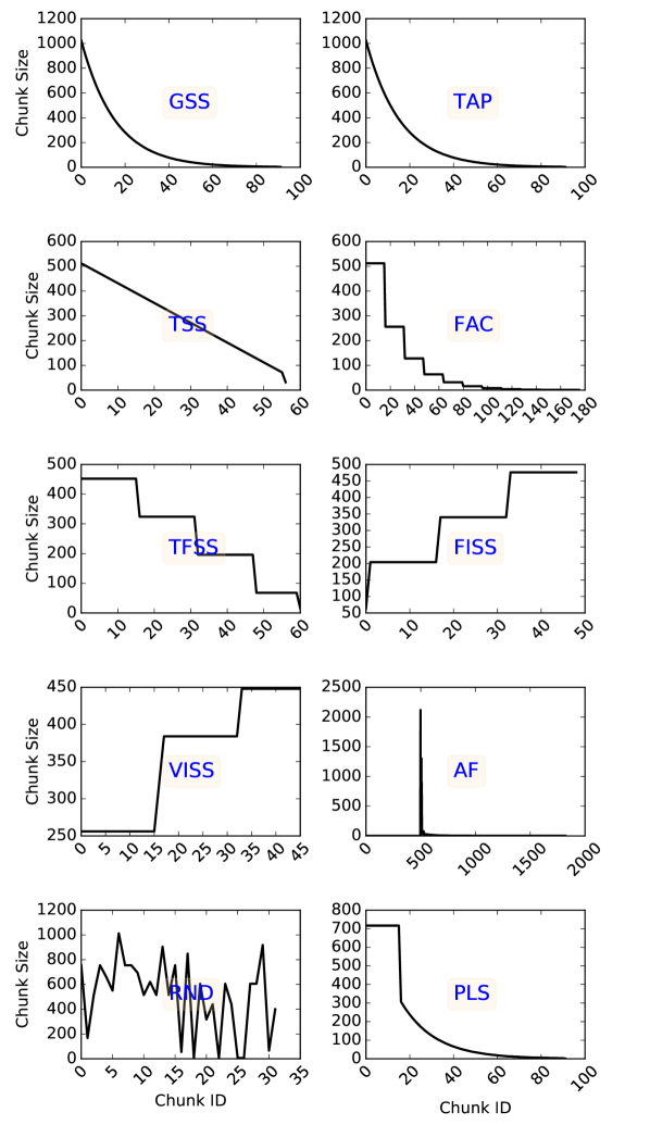
Figure 1: Example of the DLS techniques chunk sizes. The data was obtained from the main loop of Mandelbrot [20] with 1,000 loop iterations and executing on an Intel Xeon processor with 4 MPI ranks. The minimum chunk size is set to be 1 loop iteration.

Table 1: Notation used in the present work

Symbol	Description
$N$	Total number of loop iterations
$P$	Total number of processing elements
$S$	Total number of scheduling steps
$B$	Total number of scheduling batches
$i$	Index of current scheduling step, $0\leq i\leq S-1$
$b$	Index of currently scheduled batch, $0\leq b\leq B-1$
$h$	Scheduling overhead associated with assigning loop iterations
$R_{i}$	Remaining loop iterations after $i$-th scheduling step
$S_{i}$	Scheduled loop iterations after $i$-th scheduling step $S_{i}+R_{i}=N$
$lp_{\text{start}}$	Index of currently executed loop iteration, $0\leq lp_{\text{start}}\leq N-1$
$L$	A DLS technique, $L\in\{STATIC,FSC,GSS,TAP,TSS,FAC,TFSS,FISS,VISS,AF,RND,PLS\}$
$K^{L}_{0}$	Size of the largest chunk of a scheduling technique $L$
$K^{L}_{S-1}$	Size of the smallest chunk of a scheduling technique $L$
$K^{L}_{i}$	Chunk size calculated at scheduling step $i$ of a scheduling technique $L$
$p_{j}$	Processing element $j$, $0\leq j\leq P-1$
$h$	Scheduling overhead for assigning a single iteration
$\sigma_{p_{i}}$	Standard deviation of the loop iterations’ execution times executed on $p_{j}$
$\mu_{p_{i}}$	Mean of the loop iterations’ execution times executed on $p_{j}$
$T_{\text{p}}^{\text{loop}}$	Parallel execution time of the application’s parallelized loops

STATIC is a straightforward technique that divides the loop into $P$ chunks of equal size. Eq. 1 shows how STATIC calculates the chunk size. Since the scheduling overhead is proportional to the number of calculated chunk sizes, STATIC incurs the lowest scheduling overhead because it has the minimum number of chunks (only one chunk for each PE).

$$K^{STATIC}_{i}=\frac{N}{P}$$ (1)

SS [21] is a dynamic self-scheduling technique where the chunk size is always one iteration, as shown in Eq. 2. SS has the highest scheduling overhead because it has the maximum number of chunks, i.e., the total number of chunks is $N$. However, SS can achieve a highly load-balanced execution in highly irregular execution environments.

$$K^{SS}_{i}=1$$ (2)

As a middle point between STATIC and SS, FSC assumes an optimal chunk size that achieves a balanced execution of loop iterations with the smallest overhead. To calculate such an optimal chunk size, FSC considers the variability in iterations’ execution time and the scheduling overhead of assigning loop iterations to be known before applications’ execution. Eq. 3 shows how FSC calculates the optimal chunk size.

$$K^{FSC}_{i}=\frac{\sqrt{2}\cdot N\cdot h}{\sigma\cdot P\cdot\sqrt{\log{P}}}$$ (3)

GSS [2] is also a compromise between the highest load balancing that can be achieved using SS and the lowest scheduling overhead incurred by STATIC. Unlike FSC, GSS assigns decreasing chunk sizes to balance loop executions among all PEs. At every scheduling step, GSS assigns a chunk that is equal to the number of remaining loop iterations divided by the total number of PEs, as shown in Eq. 4.

$$\begin{split}&K^{GSS}_{i}=\frac{R_{i}}{P}\text{, where}\\ &R_{i}=N-\sum_{j=0}^{i-1}k^{GSS}_{j}\end{split}$$ (4)

TAP [17] is based on a probabilistic analysis that represents a general case of GSS. It considers the average of loop iterations execution time $\mu$ and their standard deviation $\sigma$ to achieve a higher load balance than GSS. Eq. 5 shows how TAP tunes the GSS chunk size based on  $\mu$ and $\sigma$.

$$\begin{split}&K^{TAP}_{i}=K^{GSS}_{i}+\frac{v^{2}_{\alpha}}{2}-v_{\alpha}\cdot\sqrt{2\cdot K^{GSS}_{i}+\frac{v^{2}_{\alpha}}{4}}\text{, where}\\ &v_{\alpha}=\frac{\alpha\cdot\sigma}{\mu}\end{split}$$ (5)

TSS [16] assigns decreasing chunk sizes similar to GSS. However, TSS uses a linear function to decrement chunk sizes. This linearity results in low scheduling overhead in each scheduling step compared to GSS. Eq. 6 shows the linear function of TSS.

$$\begin{split}&K^{TSS}_{i}=K^{TSS}_{i-1}-\left\lfloor\frac{K^{TSS}_{0}-K^{TSS}_{S-1}}{S-1}\right\rfloor\text{, where}\\ &S=\left\lceil\frac{2\cdot N}{K^{TSS}_{0}+K^{TSS}_{S-1}}\right\rceil\\ &K^{TSS}_{0}=\left\lceil\frac{N}{2\cdot P}\right\rceil\-\-,K^{TSS}_{S-1}=1\end{split}$$ (6)

FAC [3] schedules the loop iterations in batches of equally-sized chunks. FAC evolved from comprehensive probabilistic analyses and it assumes prior knowledge about $\mu$ and $\sigma$ their mean execution time. Another practical implementation of FAC denoted FAC2, assigns half of the remaining loop iterations for every batch, as shown in Eq. 7. The initial chunk size of FAC2 is half of the initial chunk size of GSS. If more time-consuming loop iterations are at the beginning of the loop, FAC2 may better balance their execution than GSS.

$$\begin{split}&K^{FAC2}_{i}=\left\{\begin{array}[]{ll}\left\lceil\frac{R_{i}}{2\cdot P}\right\rceil,\text{if}\ i\mod P=0\\ K^{FAC2}_{i-1},\text{otherwise.}\end{array}\right.\text{, where}\\ &R_{i}=N-\sum_{j=0}^{i-1}k^{FAC2}_{j}\end{split}$$ (7)

TFSS [6] combines certain characteristics of TSS [16] and FAC [3]. Similar to FAC, TFSS schedules the loop iterations in batches of equally-sized chunks. However, it does not follow the analysis of FAC, i.e., every batch is not half of the remaining number of iterations. Batches in TFSS decrease linearly, similar to chunk sizes in TSS. As shown in Eq. 8, TFSS calculates the chunk size as the sum of the next P chunks that would have been computed by the TSS divided by P.

$$K^{TFSS}_{i}=\left\{\begin{array}[]{ll}\frac{\sum_{j=i}^{i+P}K^{TSS}_{j-1}}{P}&\text{if}\ i\-\-\mod P=0\\ K^{TFSS}_{i-1},&\text{otherwise.}\end{array}\right.$$ (8)

GSS [2], TAP [17], TSS [16], FAC [3], and TFSS[6] employ a decreasing chunk size pattern. This pattern introduces additional scheduling overhead due to the small chunk sizes towards the end of the loop execution. On distributed-memory systems, the additional scheduling overhead is more substantial than on shared-memory systems. Fixed increase size chunk (FISS) [7] is the first scheduling technique devised explicitly for distributed-memory systems. FISS follows an increasing chunk size pattern calculated as in Eq. 9. FISS depends on an initial value $B$ defined by the user (suggested to be equal to the total number of batches of FAC).

$$\begin{split}&K^{FISS}_{i}=K^{FISS}_{i-1}+\lceil\frac{2\cdot N\cdot(1-\frac{B}{2+B})}{P\cdot B\cdot(B-1)}\rceil\text{, where}\\ &K^{FISS}_{0}=\frac{N}{(2+B)\cdot P}\end{split}$$ (9)

VISS [7] follows an increasing pattern of chunk sizes. Unlike FISS, VISS relaxes the requirement of defining an initial value $B$. VISS works similarly to FAC2, but instead of decreasing the chunk size, VISS increments the chunk size by a factor of two per scheduling step. Eq. LABEL:eq:viss shows the chunk calculation of VISS.

$$\begin{split}&K^{VISS}_{i}=\left\{\begin{array}[]{ll}K^{VISS}_{i-1}+\frac{K^{VISS}_{i-1}}{2}&\text{if}\ i\mod P=0\\ K^{VISS}_{i-1},&\text{otherwise.}\end{array}\right.\text{, where}\\ &K^{VISS}_{0}=K^{FISS}_{0}\end{split}$$ (10)

AF [19] is an adaptive DLS technique based on FAC. However, in contrast to FAC, AF learns both $\mu$ and $\sigma$ for each computing resource during application execution to ensure full adaptivity to all factors that cause load imbalance. AF does not follow a specific pattern of chunk sizes. AF adapts chunk size based on the continuous updates of $\mu$ and $\sigma$ during applications execution. Therefore, the pattern of AF’s chunk sizes is unpredictable. Eq. 11 shows the chunk calculation of AF.

$$\begin{split}&K^{AF}_{i}=\frac{D+2\cdot E\cdot R_{i}-\sqrt{D^{2}+4\cdot D\cdot E\cdot R_{i}}}{2\mu_{p_{i}}}\text{,where}\\ &D=\sum_{p_{i}=1}^{P}\frac{\sigma^{2}_{p_{i}}}{\mu_{p_{i}}}\\ &E=\left(\sum_{p_{i}=1}^{P}\frac{1}{\mu_{p_{i}}}\right)^{-1}\end{split}$$ (11)

RND [22] is a DLS technique that utilizes a uniform random distribution to arbitrarily choose a chunk size between specific lower and upper bounds. The lower and the upper bounds were suggested to be $\frac{N}{100\cdot P}$ and $\frac{N}{2\cdot P}$, respectively [22]. In the current work, we suggest a lower and an upper bound as $1$ and $\frac{N}{P}$, respectively. These bounds make RND have an equal probability of selecting any chunk size between the chunk size of STATIC and the chunk size of SS, which are the two extremes of DLS techniques in terms of scheduling overhead and load balancing. Eq. 12 represents the integer range of the RND chunk sizes.

$$K^{RND}_{i}\in\bigl{[}1,N/P\bigr{]}$$ (12)

PLS [18] combines the advantages of SLS and DLS. It divides the loop into two parts. The first loop part is scheduled statically. In contrast, the second part is scheduled dynamically using GSS. The static workload ratio (SWR) is used to determine the amount of the iterations to be statically scheduled. SWR is calculated as the ratio between minimum and maximum iteration execution time of five randomly chosen iterations. PLS also uses a performance function (PF) to statically assign parts of the workload to each processing element $p_{j}$ based on the PE’s speed and its current CPU load. In the present work, all PEs are assumed to have the same load during the execution. This assumption is valid given the exclusive access to the HPC infrastructure used in this work. Eq. 13 shows the chunk calculation of PLS.

$$\begin{split}&K^{PLS}_{i}=\left\{\begin{array}[]{ll}\frac{N\cdot SWR}{P},&\text{if}\ R_{i}\textgreater N-(N\cdot SWR)\\ K^{GSS}_{i},&\text{otherwise.}\end{array}\right.\text{, where}\\ &SWR=\frac{\text{minimum iteration execution time}}{\text{maximum iteration execution time}}\end{split}$$ (13)

Table 2 shows the chunk sizes generated by each technique. We obtain these chunks by assuming that the total number of iterations $N$ is 1,000 and the total number of PEs $P$ is 4. In addition to these two parameters, we consider other parameters required by each DLS technique. For instance, FSC requires the scheduling overhead $h$, which is considered to be 0.013716 seconds. TAP requires $\mu$, $\sigma$, and $\alpha$ that are assumed to be 0.1, 0.0005, and 0.0605 seconds, respectively. For FISS and VISS, we consider $B$ and $X$ to be 3 and 4. For PLS, we assume the $SWR$ ratio be 0.7.

Table 2: Chunk sizes for the selected DLS techniques considered in the current work for the main loop of Mandelbrot [20] with 1,000 loop iterations and executing on an Intel Xeon processor with 4 MPI ranks.

Technique	Chunk sizes	Total number of chunks
STATIC	250, 250, 250, 250	4
SS	1, 1, 1, $\cdots$, 1	1000
FSC	17, 17, 17, $\cdots$, 14	59
GSS	250, 188, 141, 106, 80, 60, 45, 34, 26, 19, 15, 11, 8, 6, 5, 4, 2	17
TAP	250, 188, 141, 106, 80, 60, 45, 34, 26, 19, 15, 11, 8, 6, 5, 3, 3	17
TSS	125, 117, 109, 101, 93, 85, 77, 69, 61, 53, 45, 37, 28	13
FAC	125, 125, 125, 125, 63, 63, 63, 63, 32, 32, 32, 32, 16, 16, 16, 16, 8, 8, 8, 8, 4, 4, 4, 4, 2, 2, 2, 2	28
TFSS	113, 113, 113, 113, 81, 81, 81, 81, 49, 49, 49, 49, 17, 11	14
FISS	50, 50, 50, 50, 83, 83, 83, 83, 116, 116, 116, 116, 4	13
VISS	62, 62, 62, 62, 93, 93, 93, 93, 108, 108, 108, 56	12
AF	1,1, $\cdots$, 3544, 3544, 2410, 1785, 235, 202, 179, 321, 247, 267, 197, 222, 202, 182, 157, 157, 144, 128, 126, 116, 105, 102, 86, 90, 89, 78, 72, 69, 65, 61, 57, 53, 50, 49, 45, 42, 40, 38, 36, 37, 33, 33, 29, 28, 28, 24, 23, 22, 21, 21, 19, 18, 17, 16, 16, 15, 14, 13, 12, 13, 12, 11, 11, 10, 10, 9, 9, 8, 8, 7, 7, 7, 6, 6, 5, 6, 5, 5, 5, 5, 4, 4, 4, 4, 4, 4, 3, 3, 3, 3, 3, 3, 3, 3, 2, 2, 2, 2, 2, 2, 2, 2, 2, 1, 1, $\cdots$, 1	316
RND	17, 84, 16, 36, 220, 64, 45, 81, 56, 210, 34, 29, 8, 100	14
PLS	175, 175, 175, 175, 75, 57, 43, 32, 24, 18, 14, 11, 8, 6, 5, 4, 3	17

3 DLS Implementation Approaches

In the current work, the self-scheduling aspect of the DLS techniques means that once a PE becomes free, it calculates a new chunk of loop iterations to be executed. The calculated chunk size is not associated with a specific set of loop iterations. Since the DLS techniques assume a central work queue, the PE must synchronize with all other PEs to self-assign unscheduled loop iterations. We can conclude that there are two operations at every scheduling step: (1) chunk calculation and (2) chunk assignment. In principle, only the chunk assignment requires a sort of global synchronization between all PEs, while the chunk calculation does not require synchronization and can be distributed across all PEs. In practice, existing DLS implementation approaches, especially for distributed-memory systems, do not consider the separation between chunk calculation and chunk assignment. Hence, the master-worker execution model dominates all existing DLS implementation approaches.

The distributed self-scheduling scheme (DSS) [6] is an example of employing the master-worker model to implement DLS techniques for distributed-memory systems. DSS relies on the master-worker execution model, similar to the one illustrated in Figure 2(a). DSS enables the master to consider the speed of the processing elements and their loads when assigning new chunks. DSS was later enhanced by a hierarchical distributed self-scheduling scheme (HDSS) [8] that employs a hierarchical master-worker model, as illustrated in Figure 2(b). DSS and HDSS assume a dedicated master configuration in which the master PE is reserved for handling the worker requests. Such a configuration may enhance the scalability of the proposed self-scheduling schemes. However, it results in low CPU utilization of the master. HDSS [8] suggested deploying the global-master and the local-master on one physical computing node with multiple processing elements to overcome the low CPU utilization of the master (see Figure 2(b)). DSS and HDSS were implemented using MPI two-sided communications. In both DSS and HDSS, the master is a central entity that performs both the chunk calculation and the chunk assignment.

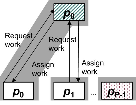
(a) Conventional master-worker execution model

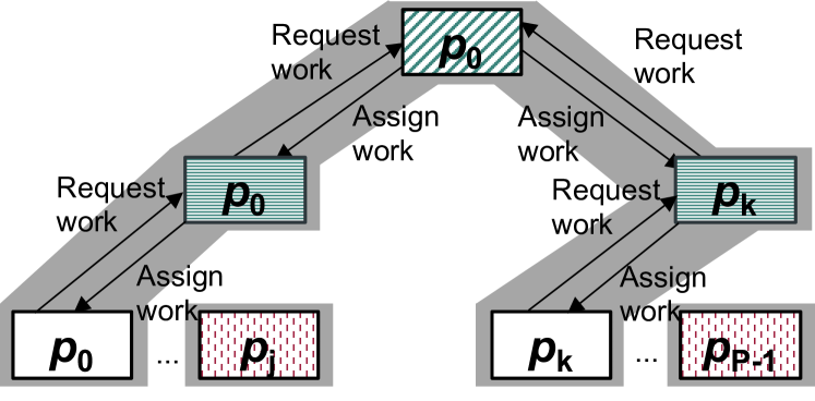
(b) Global and local masters are located on a single physical compute node

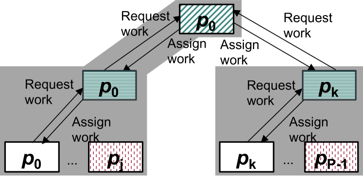
(c) Local masters are distributed across multiple physical compute nodes

Figure 2: Variants of the master-worker execution model as reported in the literature. Replication of certain processing elements is just to indicate their double role where the master participates in the computation as a worker.

Another MPI-based library that implements several DLS techniques is called the load balancing tool (LB tool) [13]. At the conceptual level, the LB tool is based on a single-level master-worker execution model (see Figure 2(a)). However, it does not assume a dedicated master. It introduces the breakAfter parameter, which is user-defined, and indicates how many iterations the master should execute before serving pending worker requests. This parameter is required for dividing the time of the master between computation and servicing of worker requests. The optimal value of this parameter is application- and system-dependent. The LB tool also employs two-sided MPI communications.

LB4MPI [14, 23] is an extension of the LB tool [13] that includes certain bug fixes and additional DLS techniques. Both LB and LB4MPI employ a master-worker execution in which the master is a central entity that performs both of chunk calculation and the chunk assignment operations.

The dynamic load balancing library (DLBL) [24] is another MPI-based library used for cluster computing. It is based on a parallel runtime environment for multicomputer applications (PREMA) [25]. DLBL is the first tool that employed MPI one-sided communication for implementing DLS techniques. Similar to the LB tool, the DLBL employs a master-worker execution model. The master expects work requests. It then calculates the size of the chunk to be assigned and, subsequently, calls a handler function on the worker side. The worker is responsible for obtaining the new chunk data without any further involvement from the master. This means that the master is still a central entity that performs both of chunk calculation and chunk assignment.

The latest advancements in the MPI 3.1 standard, namely the revised and the clear semantics of the MPI RMA (one-sided communication) [26, 27], enabled its usage in different scientific applications [28, 29, 30]. This motivated our earlier work [11] that introduced DCA. The DCA does not require the master-worker execution scheme [11]. Using MPI RMA, DCA makes one processing element, called coordinator, store global scheduling information such as the index of the latest scheduling step $i$ and the index of the previously scheduled loop iteration $lp_{start}$. The coordinator entity shares the memory address space where the global scheduling information is stored with all workers. Figure 3 shows that with certain exclusive load and store operations to the shared memory address space, all entities can simultaneously calculate and assign themselves chunks of non-overlapping loop iterations.

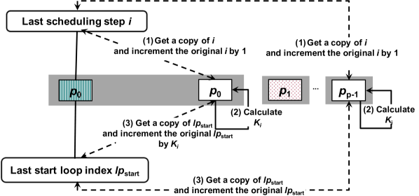
Figure 3: The distributed chunk calculation approach (DCA) using MPI RMA and passive-target synchronization.

The following question arises: Is DCA limited to specific MPI features? It is essential to answer this question because only specific MPI runtime libraries fully implement the features of the MPI 3.1 standard.

4 Distributed Chunk Calculation Approach (DCA)

The idea of DCA is to ensure that the calculated chunk size at a specific PE does not rely on any information about the chunk size calculated at any other PE. The chunk calculation formulas (Eq. 1 to 13) can be classified into straightforward and recursive. A straightforward chunk calculation formula only requires some constants and input parameters. A recursive chunk calculation formula requires information about previously calculated chunk sizes. For instance, STATIC, SS, FSC, and RND have straightforward chunk calculation formulas that do not require any information about previously calculated chunks, while GSS [2], TAP [17], TSS [16], FAC [3], TFSS [6], FISS [7], VISS [7], AF [19], and PLS [18] employ recursive chunk calculation formulas. Certain transformations have been required to convert these recursive formulas into straightforward formulas to enable DCA. For GSS and FAC, the transformations were already introduced in the literature [3] (Eq. 14 and 15).

$$K^{\prime^{GSS}}_{i}=\left\lceil\left(\frac{P-1}{P}\right)^{i}\cdot\frac{N}{P}\right\rceil$$ (14)

$$K^{\prime^{FAC2}}_{i}=\left\lceil\left(\frac{1}{2}\right)^{i_{\text{new}}}\cdot\frac{N}{P}\right\rceil,\ \ i_{\text{new}}=\left\lfloor\frac{i}{P}\right\rfloor+1$$ (15)

As shown in Eq. 5, TAP calculates $K^{GSS}_{i}$ and tunes that value based on $\mu$, $\sigma$, and $\alpha$. Based on Eq. 14, the chunk calculation formula of TSS can be expressed as a straightforward formula as follows.

$$\begin{split}&K^{\prime^{TAP}}_{i}=K^{\prime^{GSS}}_{i}+\frac{v^{2}_{\alpha}}{2}-v_{\alpha}\cdot\sqrt{2\cdot K^{\prime^{GSS}}_{i}+\frac{v^{2}_{\alpha}}{4}}\text{, where}\\ &v_{\alpha}=\frac{\alpha\cdot\sigma}{\mu}\end{split}$$ (16)

For TSS, a straightforward formula for the chunk calculation is shown in Eq. 17.

$$K^{\prime^{TSS}}_{i}=K^{TSS}_{0}-i\cdot\lfloor\frac{K^{TSS}_{0}-K^{TSS}_{S-1}}{S-1}\rfloor$$ (17)

The mathematical derivation that converts Eq. 6 into Eq. 17 is as follows. The TSS chunk calculation formula can be represented as follows, where C is a constant.

$$\begin{split}&K^{TSS}_{i}=K^{TSS}_{i-1}-C\\ &C=\left\lfloor\frac{K^{TSS}_{0}-K^{TSS}_{S-1}}{S-1}\right\rfloor\\ &K^{TSS}_{1}=K^{TSS}_{0}-C\\ &K^{TSS}_{2}=K^{TSS}_{1}-C=(K^{TSS}_{0}-C)-C=K^{TSS}_{0}-2\cdot C\\ &K^{TSS}_{i}=K^{TSS}_{0}-i\cdot C\\ &K^{TSS}_{i}=K^{TSS}_{0}-i\cdot\lfloor\frac{K^{TSS}_{0}-K^{TSS}_{S-1}}{S-1}\rfloor=K^{\prime^{TSS}}_{i}\end{split}$$

TFSS [6] is devised based on TSS [16] and FAC [3]. Therefore, the straightforward formula of TSS (see Eq. 6) can be used to derive the straightforward formula of TFSS, as shown in Eq. 18.

$$K^{\prime^{TFSS}}_{i}=\frac{\sum_{j=i}^{i+P}K^{\prime^{TSS}}_{j-1}}{P}$$ (18)

For FISS [7], a straightforward formula for the chunk calculation is shown in Eq. 19.

$$K^{\prime^{FISS}}_{i}=K^{FISS}_{0}+i\cdot\lceil\frac{2\cdot N\cdot(1-\frac{B}{2+B})}{P\cdot B\cdot(B-1)}\rceil$$ (19)

The mathematical derivation that converts Eq. 9 into Eq. 19 is as follows. Given that $A$ is a constant, the FISS chunk calculation formula can be represented as follows, where $C$ is a constant.

$$\begin{split}&K^{FISS}_{i}=K^{FISS}_{i-1}+C\\ &C=\lceil\frac{2\cdot N\cdot(1-\frac{B}{2+B})}{P\cdot B\cdot(B-1)}\rceil\\ &K^{FISS}_{1}=K^{FISS}_{0}+C\\ &K^{FISS}_{2}=K^{FISS}_{1}+C=(K^{FISS}_{0}+C)+C=K^{FISS}_{0}+2\cdot C\\ &K^{FISS}_{i}=K^{FISS}_{0}+i\cdot C\\ &K^{FISS}_{i}=K^{FISS}_{0}+i\cdot\lceil\frac{2\cdot N\cdot(1-\frac{B}{2+B})}{P\cdot B\cdot(B-1)}\rceil=K^{\prime^{FISS}}_{i}\end{split}$$

For VISS [7], a straightforward formula for the chunk calculation is shown in Eq. LABEL:eq:viss2.

$$\begin{split}&K^{\prime^{VISS}}_{i}=K^{FISS}_{0}\cdot\frac{1-(0.5)^{i_{new}}}{0.5},\text{where}\ \ i\textgreater 0\\ &i_{new}=i\mod P\\ &K^{\prime^{VISS}}_{0}=K^{FISS}_{0}\end{split}$$ (20)

To derive Eq. LABEL:eq:viss2, we calculate $K^{VISS}_{1}$, $K^{VISS}_{2}$, and $K^{VISS}_{3}$, according Eq. LABEL:eq:viss.

$$\begin{split}&K^{VISS}_{1}=K^{FISS}_{0}+\frac{K^{FISS}_{0}}{2},\text{assume}\ \ K^{FISS}_{0}=a\\ &K^{VISS}_{1}=a+\frac{a}{2}\\ &K^{VISS}_{2}=K^{VISS}_{1}+\frac{K^{VISS}_{1}}{2}=(a+\frac{a}{2})+(\frac{a+\frac{a}{2}}{2})\\ &K^{VISS}_{3}=K^{VISS}_{2}+\frac{K^{VISS}_{2}}{2}=((a+\frac{a}{2})+(\frac{a+\frac{a}{2}}{2}))+\frac{((a+\frac{a}{2})+(\frac{a+\frac{a}{2}}{2}))}{2}\\ &\text{According to the geomertic summation theorem}\\ &K^{VISS}_{i}=K^{FISS}_{0}\cdot\frac{1-(0.5)^{i}}{0.5}\\ &\text{since VISS assigns chunks in batches}\\ &K^{VISS}_{i}=K^{FISS}_{0}\cdot\frac{1-(0.5)^{i_{new}}}{0.5}=K^{\prime^{VISS}}_{i},\text{where}\ i\textgreater 0,\\ &\text{and }i_{new}=i\mod P.\\ \end{split}$$

For PLS, the loop iteration space is divided into two parts. In the first part, the PLS chunk calculation formula is equivalent to STATIC, i.e., the chunk calculation formula is a straightforward formula that is ready to support DCA. In the second part, PLS uses the GSS chunk calculation formula. Therefore, we replace $K_{i}^{GSS}$ in Eq. 13 with $K^{\prime^{GSS}}_{i}$ from Eq. 14 to derive the PLS chunk calculation (Eq. 21).

$$\begin{split}&K^{\prime^{PLS}}_{i}=\left\{\begin{array}[]{ll}\frac{N\cdot SWR}{P},&\text{if}\ R_{i}\textgreater N-(N\cdot SWR)\\ K^{\prime^{GSS}}_{i},&\text{otherwise.}\end{array}\right.\\ \end{split}$$ (21)

AF adapts the calculated chunk size according $\mu_{p_{i}}$ and $\sigma_{p_{i}}$, which can be determined only during loop execution. Moreover, at every scheduling step, AF uses $R_{i}$ with $\mu_{p_{i}}$ and $\sigma_{p_{i}}$ to calculate the chunk size. This leads to an unpredictable pattern of chunk sizes and makes it impossible to find a straightforward formula for AF. Accordingly, we could not determine a way to implement AF with a fully distributed chunk calculation. In our implementation, AF with DCA requires additional synchronization of $R_{i}$ across all PEs. All PEs can simultaneously calculate $D$ and $E$ from Eq. 11. However, each PE needs to synchronize with all other PEs to calculate each $K_{i}^{AF}$.

5 DCA implementation into LB4MPI

LB4MPI  [14, 23] is a recent MPI-based library for loop scheduling and dynamic load balancing. LB4MPI extends the LB tool [13] by including certain bug fixes and additional DLS techniques. LB4MPI has been used to enhance the performance of various scientific applications [31]. In this work, we extend the LB4MPI in two directions: (1) We enable the support of DCA. All the DLS techniques originally supported in LB4MPI were implemented with a centralized chunk calculation approach (CCA). We redesign and reimplement them with DCA. (2) We add six additional DLS techniques and implement them with CCA and DCA.

While LB4MPI schedules independent loop iterations across multiple MPI processes, it assumes that each MPI process has access to the data associated with the loop iterations it executes. The simplest way to ensure the validity of that assumption is to replicate the data of all loop iterations across all MPI processes. Users can also centralize or distribute data of the loop iterations across all MPI processes. In this case, however, users need to provide a way to their application to exchange the required data associated with the loop iterations.

The LB4MPI has six API functions: DLS_Parameters_Setup, DLS_StartLoop, DLS_Terminated, DLS_StartChunk, DLS_EndChunk, and DLS_EndLoop. One can use these API functions as in Listing 1.

#include$\textless$mpi.h$\textgreater$;
#include$\textless$LB4MPI.h$\textgreater$;

main(){

0 .../*application code*/

1 int mode = DECENTRALIZED; /*or CENTRALIZED*/

2 Configure_Chunk_Calculation_Mode($mode$);

3 DLS_Parameters_Setup($params$); /*includes number of tasks, scheduling method, scheduling parameters $\mu$, $\sigma$, $\cdots$ etc*/

4 DLS_StartLoop( info, start_index,end_index, scheduling_method );

while (!DLS_Terminated($info$)) do

      6 DLS_StartChunk($info$, $lp_{start}$, $chunk\_size$ );

      7 /*application code to process loop from $lp_{start}$ to $lp_{start}+chunk\_size$ */

      8 DLS_EndChunk($info$);

      

10DLS_EndLoop($info$, $scheduled\_tasks$, $total\_time$); }

Listing 1 Usage of LB4MPI for loop scheduling and dynamic load balancing in scientific applications

For backward compatibility reasons, our extension of LB4MPI maintained these six APIs. However, we added a new API: Configure_Chunk_Calculation_Mode that selects between CCA and DCA. We changed the functionality of each of the six APIs to include a condition that checks the selected approach (CCA or DCA) when the selected approach is CCA, the six APIs work as in the original LB4MPI. For instance, DLS_StartChunk calls either DLS_StartChunk_Centralized or DLS_StartChunk_Decentralized based on the selected approach. DLS_StartChunk_Centralized is a function that wraps the original CCA of LB4MPI, while DLS_StartChunk_Decentralized provides the newly added functionality that supports DCA.

6 Performance Evaluation and Discussion

Two computationally-intensive parallel applications are considered in this study to assess the performance potential of the proposed DCA. The first application, called PSIA [32], uses a parallel version of the well-known spin-image algorithm (SIA) [33]. SIA converts a 3D object into a set of 2D images. The generated 2D images can be used as descriptive features of the 3D object. As shown in Listing 2, a single loop dominates the performance of PSIA.

spinImagesKernel (W, B, S, OP, M);

Inputs : W: image width, B: bin size, S: support angle, OP: list of 3D points, M: number of spin-images

Output : R: list of generated spin-images

1 for  i = 0 $\rightarrow$ M do

      2 P = OP[i];

      3 tempSpinImage[W, W];

       for j = 0 $\rightarrow$ $length(OP)$ do

            5 X = OP[j];

            6 $np_{i}$ = getNormalVector(P);

            7 $np_{j}$ = getNormalVector(X);

             if acos($np_{i}\cdot np_{j}$) $\leq S$ then

                  9 $k$ = $\Bigg{\lceil}$ $\cfrac{W/2-np_{i}\cdot(X-P)}{B}$ $\Bigg{\rceil}$;

                  10 $l$ = $\Bigg{\lceil}$ $\cfrac{\sqrt{||X-P||^{2}-(np_{i}\cdot(X-P))^{2}}}{B}$ $\Bigg{\rceil}$;

                  11 if 0 $\leq$ k $\textless$ W and 0 $\leq$ l $\textless$ W then

                         tempSpinImage[k, l]++;

                        

                  

            

      16R.append(tempSpinImage);

      

Listing 2 Parallel spin-image calculations. The main loop is highlighted in the blue color.

The second application calculates the Mandelbrot set [20]. The Mandelbrot set is used to represent geometric shapes that have the self-similarity property at various scales. Studying such shapes is important and of interest in different domains, such as biology, medicine, and chemistry [34].

mandelbrotSetCalculations (W, T);

Inputs : W: image width, CT: Conversion Threshold

Output : V: Visual representation of mandelbrot set calculations

for  counter = 0 $\rightarrow$ $W^{2}$ do

      2 $x$ = counter $/$ W;

      3 $y$ = counter $\mod$ W;

      4 $c$= complex(x_min + x/W*(x_max-x_min) , y_min + y/W*(y_max-y_min));

      5 $z$ = complex(0,0) ;

      6 for $k=0\rightarrow$ $CT$ OR $|z|\textless 2.0$ do

            7 $z=z^{4}+c$;

            

      9if  $k=CT$ then

            10 set $V(x,y)$ to black;

            

      else

            13 set $V(x,y)$ to blue;

            

      

Listing 3 Mandelbrot set calculations. The main loop is highlighted in the blue color.

As shown in Listings 2 and 3, both applications contain a single large parallel loop iterations that dominates their execution times. Dynamic and static distributions of the most time-consuming parallel loop across all processing elements may enhance applications’ performance. Table 3 summarizes the characteristics of the main loops of both applications.

Table 3: Characteristics of the selected applications’ main loop

Application characteristics	Application
	PSIA	Mandelbrot
Number of loop iterations	262,144	262,144
Maximum iteration execution time (s)	0.190161	0.06237
Minimum iteration execution time (s)	0.0345	0.000001
Average iteration execution time (s)	0.07298	0.01025
Standard deviation (s)	0.00885	0.0187
Coefficient of variation (c.o.v.)	0.256	1.824

The target experimental system is called miniHPC. It consists of 26 compute nodes that are actively used for research and educational purposes. In the present work, we use sixteen dual-socket nodes. Each node has two sockets with Intel Xeon E5-2640 processors and 10 cores per socket.

For each of the two applications, we evaluate the performance of twelve different techniques with both chunk calculation approaches: DCA and CCA. Table 4 shows our design of factorial experiments in which each experiment is repeated 20 times. All applications are compiled without compiler optimization (-O0) using the Intel compiler version 19.1.0.166. The Intel MPI Library for Linux OS version 2019 (update 6) is used to execute both applications.

Table 4: Design of factorial experiments

Factor	Value
Application	PSIA #spin-images= 262,144 (Total number of loop iterations to be scheduled) image_size= 5*5 bin_size=0.01 support_angle= 0.5
	Mandelbrot image_size=512*512 (Total number of loop iterations to be scheduled) conversion_threshold= 1,000,000
Chunk calculation approach	CCA and DCA
Scheduling techniques	STATIC, FSC, GSS, TAP, TSS, FAC, TFSS, FISS, VISS, RND, AF, PLS
System	16 Xeon nodes and 16 MPI ranks per node Total of 256 MPI ranks
Injected delay	0, 10, and 100 microseconds
Experiment repetitions	20

In the present work, we evaluate the performance potential of DCA and CCA in three different scenarios. These scenarios represent cases when a slowdown affects the PEs and results in slowing down the chunk calculation. In the first scenario, no delay is injected during the chunk calculation. In the other two scenarios, a constant delay is injected in the chunk calculation. the injected delay was 10 and 100 microseconds for these two scenarios, respectively.

Figures 4 and 5 show the performance of both CCA and DCA with different techniques for PSIA and Mandelbrot, respectively. As shown in Table 3, the coefficient of variation (c.o.v.) for PSIA is significantly less than that of Mandelbrot. This low c.o.v. indicates that PSIA has less load imbalance than Mandelbrot. In Figure 4(a), using CCA, the parallel loop execution time $T_{loop}^{par}$ is 73.41 seconds with STATIC, while the best $T_{loop}^{par}$ is 69.37 with FAC. With FAC, the performance of PSIA is enhanced by 5.5%. Other techniques achieve comparable performance. For instance, $T_{loop}^{par}$ is 69.53 seconds with PLS. In contrast, other techniques degrade the performance of PSIA. GSS and RND degrade the PSIA performance by 2.7% and 61.2% compared STATIC. For the DCA, one can make the same observations regarding the best and the worst techniques. The CCA and DCA versions of all techniques are comparable to each other, i.e., the difference in performance ranges from 2% to 3%.

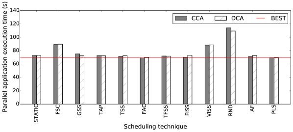
(a) Without an injected delay

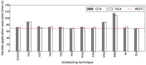
(b) With low injected delay (10 microseconds)

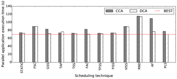
(c) With severe injected delay (100 microseconds)

Figure 4: Parallel application execution time of PSIA in the three slowdown scenarios

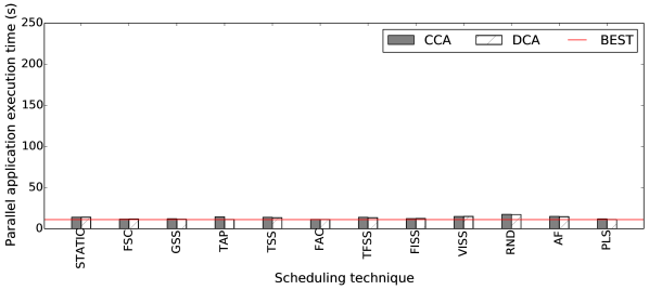
(a) Without an injected delay

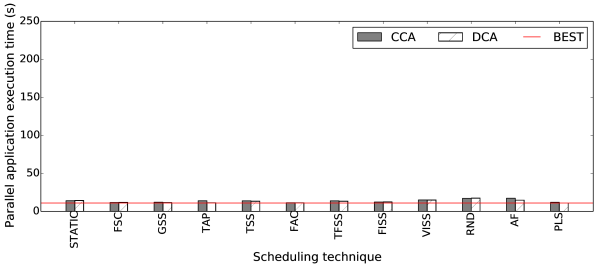
(b) With low injected delay (10 microseconds)

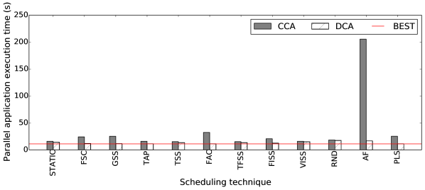
(c) With severe injected delay (10 microseconds)

Figure 5: Parallel application execution time of Mandelbrot in the three slowdown scenarios

Figures 4(b) and 4(c) show the performance of both CCA and DCA with different techniques for PSIA when the injected delay is 10 and 100 microseconds, respectively. In Figure 4(b), one can notice that when the injected delay is 10 microseconds, the performance differences between CCA and DCA with all techniques are in the range of 2% to 3%. Considering the variation in $T_{loop}^{par}$ of the 20 repetitions of each experiment, one observes that both approaches still have a comparable performance. For the largest injected delay, the DLS techniques implemented with CCA are more sensitive than the DLS techniques implemented with DCA (see Figure 4(c)). For Mandelbrot, one can notice the same behavior, i.e., when there is no injected delay or when the inject delay is 10 microseconds, the performance differences between CCA and DCA with all techniques are minor (see Figures 5(a) and 5(b)). In contrast, Figure 5(c) shows that the DCA version of all the DLS techniques is more capable of maintaining its performance than the CCA version.

Another interesting observation is the extreme poor performance of AF with CCA (see Figure 5(c)). AF is an adaptive technique, and it accounts for all sources of load imbalance that affect applications during the execution. However, AF only considers $mu_{pi}$ and $\sigma_{pi}$. Since we inject the delay in the chunk calculation function, AF cannot account for such a delay, and it works similarly to the case of no injected delay. Considering the characteristics of the Mandelbrot application, the majority of the AF chunks are equal to 1 loop iterations. This fine chunk size leads to an increased number of chunks, i.e., the performance significantly decreased because the injected delay is proportional with the total number of chunks. For PSIA, the corresponding AF implementation (with CCA) does not have the same extreme poor performance (see Figure 4(c)) because the AF chunk sizes in the case of PSIA are larger than the chunk sizes in the case of Mandelbrot.

7 Conclusion and Future Work

In the present work, we studied how the distributed chunk calculation approach (DCA) [11] can be applied to different categories of DLS techniques including DLS techniques that have fixed, decreasing, increasing, and irregular chunk size patterns. The mathematical formula of the chunk calculation of any DLS technique can either be straightforward or recursive. The DCA requires that the mathematical formula of the chunk calculation be straightforward. When one of the selected DLS techniques employs a recursive chunk calculation formula, we showed the mathematical transformations required to convert it into a straightforward formula.

By implementing the DCA in an MPI-based library called LB4MPI [14, 23] using the two-sided MPI communication that is supported by all existing MPI runtime libraries, the present work answered the question: Is DCA limited to specific MPI features?

The present work showed the performance of CCA and DCA in three different slowdown scenarios. In the first scenario, no delay was injected during the chunk calculation. In the other two scenarios, a constant delay (small and large) was injected during the chunk calculation. These scenarios represent cases when a slowdown affects the CPU and results in slowing down the chunk calculation. For these two scenarios, the injected delay was 0.00001 and 0.0001 seconds, respectively. For the large injected delay, the results showed that the DLS techniques implemented using the DCA were slightly affected by the injected delay. This confirms the performance potential of the DCA [11]. In a highly uncertain execution environment, when a slowdown affects the computational power of the coordinator (master), DCA is a better alternative to the CCA.

DCA incurs more communication messages than CCA, specifically the message required to exchange scheduling data between the coordinator and the workers. This increased number of messages could make DCA underperform CCA if the delay was injected during the chunk assignment rather than the chunk calculation. Therefore, we plan to assess the performance of DCA with various communication slowdown scenarios. Another future extension for LB4MPI is to enable dynamic selection of the scheduling approach (DCA or CCA) that minimizes applications’ execution time.

References

- [1] Z. Fang, P. Tang, P.-C. Yew, C.-Q. Zhu, Dynamic Processor Self-scheduling for General Parallel Nested Loops, IEEE Transactions on Computers 39 (7) (1990) 919–929.
- [2] C. D. Polychronopoulos, D. J. Kuck, Guided Self-Scheduling: A Practical Scheduling Scheme for Parallel Supercomputers, IEEE Transactions on Computers 100 (12) (1987) 1425–1439.
- [3] S. Flynn Hummel, E. Schonberg, L. E. Flynn, Factoring: A Method for Scheduling Parallel Loops, Communications of the ACM 35 (8) (1992) 90–101.
- [4] D. J. Becker, T. Sterling, D. Savarese, J. E. Dorband, U. A. Ranawak, C. V. Packer, BEOWULF: A Parallel Workstation for Scientific Computation, in: Proceedings of the International Conference on Parallel Processing, Vol. 95, 1995, pp. 11–14.
- [5] K. Castagnera, D. Cheng, R. Fatoohi, E. Hook, B. Kramer, C. Manning, J. Musch, C. Niggley, W. Saphir, D. Sheppard, et al., Clustered Workstations and Their Potential Role as High Speed Compute Processors, NAS Computational Services Technical Report RNS-94-003, NAS Systems Division, NASA Ames Research Center.
- [6] A. T. Chronopoulos, R. Andonie, M. Benche, D. Grosu, A Class of Loop Self-scheduling for Heterogeneous Clusters, in: Proceedings of International Conference on Cluster Computing, 2001, pp. 282–291.
- [7] T. Philip, C. R. Das, Evaluation of Loop Scheduling Algorithms on Distributed Memory Systems, in: Proceedings of the International Conference on Parallel and Distributed Computing Systems, 1997, pp. 76–94.
- [8] A. T. Chronopoulos, S. Penmatsa, N. Yu, D. Yu, Scalable Loop Self-scheduling Schemes for Heterogeneous Clusters, International Journal of Computational Science and Engineering 1 (2-4) (2005) 110–117.
- [9] I. Banicescu, V. Velusamy, J. Devaprasad, On the Scalability of Dynamic Scheduling Scientific Applications with Adaptive Weighted Factoring, Journal of Cluster Computing 6 (3) (2003) 215–226.
- [10] R. L. Cariño, I. Banicescu, Dynamic Load Balancing With Adaptive Factoring Methods in Scientific Applications, The Journal of Supercomputing 44 (1) (2008) 41–63.
- [11] A. Eleliemy, F. M. Ciorba, Dynamic Loop Scheduling Using MPI Passive-Target Remote Memory Access, in: Proceedings of the 27th Euromicro International Conference on Parallel, Distributed and Network-based Processing, 2019, pp. 75–82.
- [12] A. Eleliemy, F. M. Ciorba, Hierarchical Dynamic Loop Self-Scheduling on Distributed-Memory Systems Using an MPI+MPI Approach, in: Proceedings of the International Parallel and Distributed Processing Symposium Workshops, 2019, pp. 689–697.
- [13] R. L. Cariño, I. Banicescu, A Load Balancing Tool for Distributed Parallel Loops, Journal of Cluster Computing 8 (4) (2005) 313–321.
- [14] A. Mohammed, A. Eleliemy, F. M. Ciorba, F. Kasielke, I. Banicescu, An Approach for Realistically Simulating the Performance of Scientific Applications on high Performance Computing Systems, Future Generation Computer Systems 111 (2020) 617–633.
- [15] C. P. Kruskal, A. Weiss, Allocating Independent Subtasks on Parallel Processors, IEEE Transactions on Software Engineering SE-11 (10) (1985) 1001–1016.
- [16] T. H. Tzen, L. M. Ni, Trapezoid Self-Scheduling: A Practical Scheduling Scheme for Parallel Compilers, IEEE Transactions on parallel and distributed systems 4 (1) (1993) 87–98.
- [17] S. Lucco, A Dynamic Scheduling Method for Irregular Parallel Programs, in: Proceedings of the ACM Conference on Programming Language Design and Implementation, 1992, pp. 200–211.
- [18] W. Shih, C. Yang, S. Tseng, A Performance-based Parallel Loop Scheduling on Grid Environments, The Journal of Supercomputing 41 (3) (2007) 247–267.
- [19] I. Banicescu, Z. Liu, Adaptive Factoring: A Dynamic Scheduling Method Tuned to the Rate of Weight Changes, in: Proceedings of th High performance computing Symposium, 2000, pp. 122–129.
- [20] B. B. Mandelbrot, Fractal Aspects of the Iteration of z→ z (1-z) for Complex and z, Annals of the New York Academy of Sciences 357 (1) (1980) 249–259.
- [21] T. Peiyi, Y. Pen-Chung, Processor Self-scheduling for Multiple-nested Parallel Loops, in: Proceedings of the International Conference on Parallel Processing, 1986, pp. 528–535.
- [22] F. M. Ciorba, C. Iwainsky, P. Buder, OpenMP Loop Scheduling Revisited: Making a Case for More Schedules, in: Proceedings of the 2018 International Workshop on OpenMP, 2018, pp. 21–36.
- [23] A. Mohammed, F. M. Ciorba, SimAS: A Simulation-assisted Approach for the Scheduling Algorithm Selection Under Perturbations, Concurrency and Computation: Practice and Experience 32 (15) (2020) e5648.
- [24] I. Banicescu, R. L. Cariño, J. P. Pabico, M. Balasubramaniam, Design and Implementation of a Novel Dynamic Load Balancing Library for Cluster Computing, Journal of Parallel Computing 31 (7) (2005) 736–756.
- [25] K. Barker, A. Chernikov, N. Chrisochoides, K. Pingali, A Load Balancing Framework for Adaptive and Asynchronous Applications, IEEE Transactions on Parallel and Distributed Systems 15 (2) (2004) 183–192.
- [26] T. Hoefler, J. Dinan, R. Thakur, B. Barrett, P. Balaji, W. Gropp, K. Underwood, Remote Memory Access Programming in MPI-3, ACM Transactions on Parallel Computing 2 (2) (2015) 9.
- [27] X. Zhao, P. Balaji, W. Gropp, Scalability challenges in current MPI one-sided implementations, in: International Symposium on Parallel and Distributed Computing (ISPDC), 2016, pp. 38–47.
- [28] J. R. Hammond, S. Ghosh, B. M. Chapman, Implementing OpenSHMEM using MPI-3 one-sided communication, in: Proceedings of the Workshop on OpenSHMEM and Related Technologies, 2014, pp. 44–58.
- [29] H. Shan, S. Williams, Y. Zheng, W. Zhang, B. Wang, S. Ethier, Z. Zhao, Experiences of Applying One-sided Communication to Nearest-neighbor Communication, in: Proceedings of the First Workshop on PGAS Applications, 2016, pp. 17–24.
- [30] H. Zhou, J. Gracia, Asynchronous progress design for a MPI-based PGAS one-sided communication system, in: Proceedings of the International Conference on Parallel and Distributed Systems, 2016, pp. 999–1006.
- [31] A. Mohammed, A. Cavelan, F. M. Ciorba, R. M. Cabezón, I. Banicescu, Two-level Dynamic Load Balancing for High Performance Scientific Applications, in: Proceedings of SIAM Parallel Processing (SIAM PP 2020), 2020, pp. 69–80.
- [32] A. Eleliemy, M. Fayze, R. Mehmood, I. Katib, N. Aljohani, Loadbalancing on Parallel Heterogeneous Architectures: Spin-image Algorithm on CPU and MIC, in: Proceedings of the 9th EUROSIM Congress on Modelling and Simulation, 2016, pp. 623–628.
- [33] A. E. Johnson, Spin-Images: A Representation for 3-D Surface Matching, Ph.D. thesis, Robotics Institute, Carnegie Mellon University (August 1997).
- [34] P. Jovanovic, M. Tuba, D. Simian, A new visualization algorithm for the Mandelbrot set, in: Proceedings of the 10th WSEAS International Conference on Mathematics and Computers in Biology and Chemistry, 2009, pp. 162–166.