Time-Efficient and High-Quality Graph Partitioning for Graph Dynamic Scaling

Abstract

The dynamic scaling of distributed computations plays an important role in the utilization of elastic computational resources, such as the cloud. It enables the provisioning and de-provisioning of resources to match dynamic resource availability and demands. In the case of distributed graph processing, changing the number of the graph partitions while maintaining high partitioning quality imposes serious computational overheads as typically a time-consuming graph partitioning algorithm needs to execute each time repartitioning is required.

In this paper, we propose a dynamic scaling method that can efficiently change the number of graph partitions while keeping its quality high. Our idea is based on two techniques: preprocessing and very fast edge partitioning, called graph edge ordering and chunk-based edge partitioning, respectively. The former converts the graph data into an ordered edge list in such a way that edges with high locality are closer to each other. The latter immediately divides the ordered edge list into an arbitrary number of high-quality partitions. The evaluation with the real-world billion-scale graphs demonstrates that our proposed approach significantly reduces the repartitioning time, while the partitioning quality it achieves is on par with that of the best existing static method.

1 Introduction

Graph analysis is a powerful method to gain valuable insights into the characteristics of real networks, such as web graphs and social networks. To analyze large-scale graphs efficiently, one of the major approaches is to distribute the entire graph across multiple machines and process each partition in parallel. Over the last decade, several distributed graph-processing systems have been developed malewicz2010pregel ; gonzalez2014graphx ; joseph2012powergraph ; hong2015pgx ; Chen:2015:PDG:2741948.2741970

For efficient parallel computation on a distributed graph-processing system, the common problem is to divide the input graph into $k$ parts in such a way that the number of edge/vertex cuts (i.e., communication cost among the distributed processes) becomes minimal while keeping each part balanced; this is known as the balanced $k$-way graph partitioning. Since the computation of the optimal-quality partitions, namely, partitions with the minimum cuts, is an NP-hard problem garey1974some ; Andreev:2004:BGP:1007912.1007931 ; Bourse:2014:BGE:2623330.2623660 ; Zhang:2017:GEP:3097983.3098033 , the high-quality graph partitioning algorithms, such as METIS Karypis:1998:FHQ:305219.305248 and NE Zhang:2017:GEP:3097983.3098033 , are generally time-consuming compared to the low-quality ones, such as FENNEL Tsourakakis:2014:FSG:2556195.2556213 , DBH NIPS2014_5396 , HDRF Petroni:2015:HSP:2806416.2806424 . There is a clear trade-off between partitioning efficiency and quality.

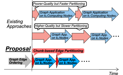
Figure 1: Workload Example. # partitions is $k_{0}\rightarrow k_{1}\rightarrow...$.

In a related development, with the utilization of elastic infrastructures such as cloud platforms, dynamic scaling of computational resources has become increasingly important for parallel and distributed computation. Especially, one of our motivated scenarios for the cloud is the effective utilization of unreliable VM instances that do not have any lifetime guarantee, such as Spot Instances in AWS spotinstance and Preemptible VMs in GCE preemptible . In such an unreliable VM environment, the price and availability of the VM is changed depending on spare resources of a data center. The spare VM resources may be suddenly available while the executing VMs may be forcely terminated by the infrastructure side. Dynamic scaling plays an important role to handle such a dynamic change of computational resources.

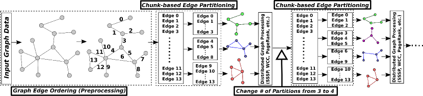
Figure 2: Dynamic Scaling based on Graph Edge Ordering and Chunk-based Edge Partitioning.

In the case of distributed graph analysis, however, scaling the number of graph partitions efficiently while achieving high quality is a challenging endeavor due to the trade-off between efficiency and quality. On the one hand, several dynamic scaling methods based on efficient graph partitioning have been proposed pujol2011little ; vaquero2014adaptive ; 8798698 ; 8514898 ; dynamicscaling , which, however, exhibit limited quality. It results in high communication costs, affecting the performance of distributed graph processing, as shown in the top of Figure 1. On the other hand, conventional approaches based on high-quality graph partitioning, e.g.,  Karypis:1998:FHQ:305219.305248 ; Zhang:2017:GEP:3097983.3098033 , may cause redundant computation as typically time-consuming calculations are required each time the number of partitions is changed, as shown in the middle of Figure 1.

The problem of graph dynamic scaling is similar to the dynamic load balancing for the distributed graph analysis shang2013catch ; khayyat2013mizan ; xu2014loggp ; huang2016leopard ; zheng2016paragon ; zheng2016planar as both need to repartition a graph. However, these methods focus on repartitioning the graph to reflect changes in the behavior of the application workload only and do not consider dynamic changes of the computational infrastructure. Furthermore, in these cases, the number of graph partitions does not change. In this paper, we focus on a different problem, where the dynamic scaling of the graph is triggered by the dynamic scaling of the computational infrastructure rather than the application workload. In such cases, the graph has to be repartitioned to make use of the newly available computational resources.

In this paper, we propose a novel approach to the dynamic scaling of graph partitions, which enables us to efficiently recompute the partitioning when the number of partitions is changed while keeping partitioning quality high. As with the latest work dynamicscaling , we focus on (vertex-cut) edge partitioning rather than traditional (edge-cut) vertex partitioning, as discussed in the other existing work pujol2011little ; vaquero2014adaptive ; 8798698 ; 8514898 . The edge partitioning is known to provide a better workload balance because the computational cost in the graph processing essentially depends on the number of edges rather than that of vertices joseph2012powergraph ; gonzalez2014graphx .

The dynamic scaling method which we propose in this paper is based on two techniques: graph edge ordering and chunk-based edge partitioning. Figure 2 shows an overview. The graph edge ordering is a preprocessing method, which orders the edges of the input graph in such a way that edges with closer ids have a higher access locality (e.g., input edges are ordered to Edge 0,1,2,3… in Figure 2). Then, the chunk-based edge partitioning, which is a simple yet very fast partitioning method, splits the ordered edge lists. Once the ordering is computed, the result can be reused, and time-consuming processing is unnecessary to repeat when the number of partitions is changed.

The contributions of this paper are as follows:

A Novel Approach to Efficient and Effective Dynamic Scaling of Graph Edge Partitions.
We formalize the dynamic scaling problem for graph edge partitions as the maximization of both efficiency and quality. Then, we propose an efficient and effective dynamic scaling approach based on chunk-based edge partitioning and graph edge ordering (Sec. 3). The efficiency is theoretically maximized as we show that the chunk-based edge partitioning is $\mathcal{O}(1)$ while the quality is theoretically guaranteed by the upper bound obtained by the graph edge ordering.

A Fast Graph Edge Ordering Algorithm.
We formalize the graph edge ordering problem as an optimization problem and show its NP-hardness. To address the NP-hard problem, we propose an efficient $\mathcal{O}(n\log n)$ greedy algorithm based on a greedy expansion. To enhance the greedy expansion, we propose a novel priority-queue which is significantly effective for the graph edge ordering problem. We show that partitions generated by the graph edge ordering and the chunk-based edge partitioning have a theoretical upper bounds of the partitioning quality. The theoretical result is similar to the best existing static method (Sec. 4).

A Comprehensive Quantitative Evaluation.
By using large-scale real-world graphs, we evaluate the efficiency and quality of our method and compare it with state-of-the-art dynamic scaling, graph partitioning, and graph ordering methods. The evaluation shows that the chunk-based edge partitioning is practically between three to eight orders of magnitude faster than the existing methods while achieving comparable quality to that of the best existing static method. As a result, the high-quality partitions obtained by our method significantly improve the performance of typical benchmarking applications (Sec. 6).

2 Preliminaries and Related Work

2.1 Notation

Let $G=(V,E)$ be an undirected and unweighted graph that consists of a set of vertices $V$ and a set of edges $E$, respectively. For $E$, the set of its $k$ disjoint subsets are represented as $\mathcal{E}_{k}:=\{\mathcal{E}_{k}[p]:0\leq p<k,\mathcal{E}_{k}[p]\subset E,\mathcal{E}_{k}[i]\cap\mathcal{E}_{k}[j]=\varnothing\ \text{for}\ i\neq j\}$. An edge $e$ $(\in E)$ connecting vertex $v$ and $u$ is represented by $e_{v,u}$. $N(v)$ represents the set of $v$’s neighboring vertices. The vertex set involved in $E$ is defined as $V(E)$, that is, $V(E):=\{v\ |\ v\in V,\exists e_{v,u}\in E\}$. The number of elements in a set is represented by $|\cdot|$, e.g., $|V|$ and $|E|$.

In this paper, we are interested in the order of elements in $E$. Let $\phi:~{}E~{}\mapsto~{}\{0,1,2,...,|E|\!-\!1\}$ be a bijective function taking an edge $e$ $(\in E)$ and returning an index $i$ $(0\leq i<|E|)$. We refer to $\phi$ as an ordering function. A list (i.e., an ordered set) of $E$ ordered by $\phi$ is represented as $E^{\phi}$. The $i$-th element in $E^{\phi}$ is represented as $E^{\phi}[i]$. We also define an append operation for the ordered edges, represented by $+$.

For example, suppose $A:=\{A[0],A[1],A[2]\}$ and $B:=\{B[0],B[1]\}$, then $(A+B)[0]:=A[0]$; $(A+B)[1]:=A[1]$; $(A+B)[2]:=A[2]$; $(A+B)[3]:=B[0]$; and $(A+B)[4]:=B[1]$.

Notation which we frequently use through the paper is summarized in Table 1.

Table 1: Summary of Notation

Symbol	Description
$V$, $E$, $G(V,E)$	Vertices, edges, and a graph with $V$ and $E$
$N(v)$	$v$’s neighbor vertices
$V(E)$	Vertices involved in $E$
$k$	# of edge partitions
$p$	Partition id ($0\leq p<k$)
$\mathcal{E}_{k}$, $\mathcal{E}_{k}[p]$	Set of edge partitions and its $p$-th edge partition
$\phi$	Ordering function
$E^{\phi}$, $E^{\phi}[i]$	Edge list ordered by $\phi$ and its $i$-th element
$\mathit{E^{\phi}_{\mathit{ch}}}(i,w)$	Chunk with $w$ edges from $i$-th edge (§ 3.3)
ID2P${}_{k}(\cdot)$	Conversion from Order $i$ to Partition $p$ (§ 3.4)

2.2 Graph Edge Partitioning

The edge partitioning algorithm divides a set of edges $E$ into $k$ disjoint subsets $\mathcal{E}_{k}$. The edge partitioning is to find partitions where the communication cost among the partitions becomes as small as possible while keeping the size of each subset balanced. In the edge partitioning, the communication occurs at boundary vertices, which are replicated into multiple partitions. Specifically, the number of boundary vertices causing the communication is represented as $\sum_{p=0}^{k-1}|V\bigl{(}\mathcal{E}_{k}[p]\bigr{)}|-|V|$. For evaluating the communication cost, a normalized factor, called replication factor (RF) joseph2012powergraph , is typically used:

Definition 1 (Replication Factor)

$$\mathit{RF}\bigl{(}\mathcal{E}_{k}\bigr{)}:=\frac{1}{|V|}\sum_{p=0}^{k-1}|V\bigl{(}\mathcal{E}_{k}[p]\bigr{)}|$$

Based on $RF$, the edge partitioning problem joseph2012powergraph is defined as follows:

Definition 2 (Balanced $k$-way Edge Partitioning)

The objective of the balanced $k$-way edge partitioning of $\boldsymbol{G}$ is formalized as follows:

$$\min_{\mathit{part}\in\mathcal{P}}RF\bigl{(}\mathit{part}(E,k)\bigr{)}\ \ \ \text{s.t.}\ \ \max_{0\leq p<k}|\mathcal{E}_{k}[p]|<(1+\epsilon)\frac{|E|}{k},$$

where $\mathit{part}:(E,k)\mapsto\{\mathcal{E}_{k}[p]:p=0,1,...,k\!-\!1\}$ is a partitioning method, and $\mathcal{P}$ is the set of all partitioning methods. The balance factor $\epsilon\geq 0$ is a constant parameter.

2.3 Related Work

Dynamic Scaling of Graph Partitions. The dynamic scaling has been extensively investigated for various distributed applications, such as web applications chieu2009dynamic ; shen2011cloudscale , database systems das2011albatross ; Das:2013:EES:2445583.2445588 ; taft2014store ; serafini2014accordion ; adya2016slicer ; taft2018p ; marcus2018nashdb , streaming systems ishii2011elastic ; shen2011cloudscale ; castro2013integrating ; heinze2015online ; madsen2017integrative ; floratou2017dhalion ; Borkowski:2019:MCR:3317315.3329476 ; Wang:2019:ERE:3299869.3319868 , data analysis shen2011cloudscale , scientific applications mao2011auto , and machine learning qiao2018litz . The major difference from these efforts is that distributed graph applications are typically communication-intensive workloads. Thus, our work focuses on the quality of the partitioning as well as the efficiency of the dynamic scaling.

The dynamic scaling for the traditional vertex graph partitioning has been studied in some work pujol2011little ; vaquero2014adaptive ; 8798698 ; 8514898 . The main difference from these efforts is that our proposal is based on edge partitioning. Our chunk-based edge partitioning makes full use of the edge partitioning so that its time complexity becomes $\mathcal{O}(1)$. Achieving $\mathcal{O}(1)$ for vertex partitioning is a very challenging endeavor (if at all possible).

The work, which appears to be closer to ours, is dynamicscaling . To the best of our knowledge, this is the only one to discuss the dynamic scaling of edge partitions. In this paper, the authors confirm that the minimization of the migration cost in dynamic scaling is NP-complete. They propose an approximate algorithm and a generic scheme based on consistent hashing. The hashing does not take into account the data locality. As a result, the quality of partitioning is not considered. In contrast, our approach aims to achieve also high partitioning quality due to the preprocessing (i.e., graph edge ordering) as compared theoretically in Sec. 5 and empirically in Sec. 6.

Graph Ordering. Due to the structural complexity of the real-world networks, it is difficult to grasp data locality among each graph element. The graph ordering is one of the major approaches to increase the data locality zhao2020graph . The most traditional method is Reverse Cuthill McKee (RCM) for matrix bandwidth reduction Cuthill:1969:RBS:800195.805928 . Different algorithms have a different focus, such as graph compression boldi2011layered ; lim2014slashburn ; dhulipala2016compressing , CPU-cache utilization wei2016speedup ; arai2016rabbit , and graph databases Goonetilleke:2017:ELS:3085504.3085516 . Our work is the first attempt to utilize the graph ordering technique for the graph partitioning problem and provides the best partitioning quality as compared in Sec. 6.

3 Proposed Dynamic Scaling Method

In this section, we first provide a formal definition of the problem. Second, we outline our our approach which is based on preprocessing the graph. Third, we present the chunk-based edge partitioning algorithm. Finally, we introduce the graph edge ordering algorithm.

3.1 Problem Definition

We formalize the dynamic scaling problem as a multi-objective problem: (i) to maximize the efficiency of the scaling and (ii) to minimize the replication factor of edge partitions generated by the scaling.

Let the number of initial partitions be $k$; the partitioned edge sets be $\mathcal{E}_{k}$; the number of added/removed computing unit be $x$.

Definition 3 (Dynamic Scaling)

Scaling in/out, $\boldsymbol{sc(\mathcal{E}_{k},\pm x)}$, is to recompute new $k\pm x$ edge partitions, $\mathcal{E}_{k\pm x}$ ($\mathcal{E}_{k\pm x}:=sc(\mathcal{E}_{k},\pm x)$).

The objective of the dynamic scaling problem for $\boldsymbol{\mathcal{E}_{k}}$ is to maximize the efficiency of the scaling ($\mathit{sc}$) and to minimize the replication factor ($RF$) as follows:

$$\max_{\mathit{sc}\in\mathcal{SC}}\mathit{EF}(\mathit{sc}(\mathcal{E}_{k},\pm x)),\ \min_{\mathit{sc}\in\mathcal{SC}}RF\bigl{(}sc(\mathcal{E}_{k},\pm x)\bigr{)}$$

$$\text{s.t.}\max_{0\leq p<k\pm x}|\mathcal{E}_{k\pm x}[p]|<(1+\epsilon)\frac{|E|}{k\pm x},$$

where $RF(sc)$ is the replication factor of the new partitions after $sc$, and the efficiency ($\mathit{EF}$) is evaluated by the time complexity to calculate partition IDs of edges.

Note that, in a similar way to the state-of-the-art work dynamicscaling , we focus on the dynamic scaling of static graphs, where the structure of the graph does not change over time. In this case, the graph is static, while the number of partitions changes dynamically to reflect changes in the underlying computational infrastructure.

3.2 Overview of Proposed Approach

We address the two objectives above one by one. Specifically, at first, the efficiency is maximized as we design the very fast $\mathcal{O}(1)$ graph partitioning method. Then, the quality is maximized by preprocessing of an input graph.

The overall computation consists of five steps as shown in Figure 2. (i) and (ii) are executed once, whereas (iii) – (v) are repeated:

• Graph Edge Ordering: The graph-edge-ordering algorithm converts the original graph data into the ordered edge list.

• Initial Partitioning to $k$ Parts: The chunk-based edge partitioning initially computes $k$ edge partitions of the ordered edge list. The graph elements (i.e., vertices and edges) are distributed to $k$ machines accordingly.

• Resource Provisioning / De-provisioning: $x$ computational units are added/removed (e.g., add/remove machine(s), CPU core(s), or CPU Socket(s)).

• Scaling to $k\pm x$ Parts: The chunk-based edge partitioning computes the $k\pm x$-way edge partitions for the ordered edge list. The additional graph elements are moved from the other processes or reloaded from the storage.

• Graph Application: Distributed graph applications are executed on the $k\pm x$ machines.

3.3 Chunk-based Edge Partitioning

The chunk-based edge partitioning evenly splits the ordered edge list into continuous chunks of edges. Specifically, the chunk-based edge partitioning algorithm for $p$-th part $(0\leq p<k)$ takes 3 arguments: (i) the ordered edge list, $E^{\phi}$, (ii) the partition ID, $p$, (iii) the total number of partitions, $k$; and returns a disjoint edge set, $\mathcal{E}_{k}[p]$, in such a way that:

$$\mathcal{E}_{k}[p]=\mathit{E^{\phi}_{\mathit{ch}}}\left(\sum_{x=0}^{p-1}\left\lfloor\tfrac{|E|+x}{k}\right\rfloor,\left\lfloor\tfrac{|E|+p}{k}\right\rfloor\right),$$

where $\mathit{E^{\phi}_{\mathit{ch}}}(\cdot,\cdot)$ is the edge chunk. We define it using its beginning point $i$ and chunk size $w$ as follows:

$$\mathit{E^{\phi}_{\mathit{ch}}}(i,w) := \{E^{\phi}[i],E^{\phi}[i+1],...,E^{\phi}[i+w-1]\}.$$

There are two noted things. First, the chunk-based edge partitioning always provides the perfect edge balance, i.e., $\epsilon\approx 0$ in Def. 2. Second, if $|E|\text{ mod }k=0$, then $\mathcal{E}_{k}[p]$ is simplified as

$$\mathcal{E}_{k}[p]=\mathit{E^{\phi}_{\mathit{ch}}}\left(\tfrac{|E|}{k}p,\tfrac{|E|}{k}\right).$$

Figure 3: Chunk-based Edge Partitioning of $E$ into 4 parts ($k=4$, $p=0,1,2,3$, and $E=\{E^{\phi}[0],E^{\phi}[1],...E^{\phi}[13]\}$).

Figure 3 shows the example of the chunk-based edge partitioning for $E=\{E^{\phi}[0],E^{\phi}[1],...E^{\phi}[13]\}$ and $k=4$. The 14 edges are divided into 3 + 3 + 4 + 4 edges because $\left\lfloor\tfrac{|E|+p}{k}\right\rfloor$ for each $p\ (0\leq p<k)$ is equal to $\left\lfloor\tfrac{14+0}{4}\right\rfloor=3$, $\left\lfloor\tfrac{14+1}{4}\right\rfloor=3$, $\left\lfloor\tfrac{14+2}{4}\right\rfloor=4$, and $\left\lfloor\tfrac{14+3}{4}\right\rfloor=4$, respectively. Therefore, $\mathcal{E}_{k}[p]$ becomes $\mathcal{E}_{4}[0]=E^{\phi}_{ch}(0,3)$, $\mathcal{E}_{4}[1]=E^{\phi}_{ch}(3,3)$, $\mathcal{E}_{4}[2]=E^{\phi}_{ch}(6,4)$, and $\mathcal{E}_{4}[3]=E^{\phi}_{ch}(10,4)$, respectively.

Since the chunk-based partitioning just splits the edge list, the computational time complexity excluding the graph data movement is basically $\mathcal{O}(1)$.

Theorem 3.1 (Efficiency of Partitioning)

Suppose the edges of $E^{\phi}$ are stored continuously (e.g., to an array or a file system), and an operation to find the pointer of $E^{\phi}[i]$ by using $i$ is $\mathcal{O}(1)$ (e.g., RAM or standard file systems). Then, there exists an $\mathcal{O}(1)$ algorithm to compute the chunk-based edge partitioning excluding the graph data movement, and it does not depend on the graph size, such as $|V|$ and $|E|$.

Proof

In order to compute the chunk-based edge partitioning in $\mathcal{O}(1)$, the algorithm needs to calculate
$\sum_{x=0}^{p-1}\left\lfloor\tfrac{|E|+x}{k}\right\rfloor$ in $\mathcal{O}(1)$. $\sum_{x=0}^{p-1}\left\lfloor\tfrac{|E|+x}{k}\right\rfloor$ requires $\mathcal{O}(p)$ computational time in a naive way.

The summation can be modified as follows:

$$\sum_{x=0}^{p-1}\left\lfloor\tfrac{|E|+x}{k}\right\rfloor=\sum_{x=0}^{p-1}\left\{\left\lfloor\tfrac{|E|}{k}\right\rfloor+\left\lfloor\tfrac{(|E|\text{ mod }k)+x}{k}\right\rfloor\right\}$$

Here, $\left\lfloor\tfrac{(|E|\text{ mod }k)+x}{k}\right\rfloor$ is $0$ or $1$ in $x=0,1,...,p-1$, as follows:

$$\left\lfloor\tfrac{(|E|\text{ mod }k)+x}{k}\right\rfloor=\begin{cases}0&\text{ if }(|E|\text{ mod }k)+x<k\\ 1&\text{ otherwise}\end{cases}$$

Therefore,

$$\sum_{x=0}^{p-1}\left\lfloor\tfrac{(|E|\text{ mod }k)+x}{k}\right\rfloor = \begin{cases}0\ \ \ \text{ if }k+(|E|\text{ mod }k)\geq p\\ p-k+(|E|\text{ mod }k)\ \ \ \text{ otherwise}\end{cases}$$

$$= \max\big{(}0,p-k+\left(|E|\text{ mod }k\right)\big{)}$$

We define $\theta_{k}(p):=\max\big{(}0,p-k+\left(|E|\text{ mod }k\right)\big{)}$. Then, the following formula is established:

$$\sum_{x=0}^{p-1}\left\lfloor\tfrac{|E|+x}{k}\right\rfloor=p\left\lfloor\tfrac{|E|}{k}\right\rfloor+\theta_{k}(p).$$

This can be computed in $\mathcal{O}(1)$. ∎

According to dynamicscaling , the migration cost is defined as the number of migrated edges. The migration cost for the chunk-based edge partitioning is provided as follows:

Theorem 3.2 (Migration Cost)

Suppose a set of ordered edges is initially split into $k$ partitions via the chunk-based edge partitioning, and the edges are repartitioned into $k+x$ parts by adding $x$ new processes (i.e., scale out). We assume that $|E|$ is much larger than $k$ and $x$ such that $(|E|\mod k+x)/|E|<(k+x)/|E|\approx 0$ and that the ids of new partitions are $k,k+1,...,k+x-1$.

Then, the approximate number of migrated edges when applying repartitioning is

$$\frac{x|E|}{2k(k+x)}\left\lceil\frac{k}{x}\right\rceil\left(\left\lceil\frac{k}{x}\right\rceil+1\right)+\frac{|E|}{k}\left(k-\left\lceil\frac{k}{x}\right\rceil\right).$$

The cost for scaling in is the same (i.e., from $k+x$ to $k$ partitions) since it is a reverse operation of scaling out.

Proof

We consider a simple case where $|E|\mod k=0,|E|\mod(k+1)=0,|E|\mod(k+2)=0,...,\ |E|\mod(k+x)=0$. Then, there are two cases in the edge migration for partition $i(i\in[0,k))$: (i) some of the edges in partition $i$ are migrated to other partitions, or (ii) all of the edges in partition $i$ are migrated to other partitions.

Case (i): In this case, for partition $i$, the edges from $i\frac{|E|}{k}$-th edge to $(i+1)\frac{|E|}{k+x}$-th are kept in partition $i$, while from $(i+1)\frac{|E|}{k+x}$-th to $(i+1)\frac{|E|}{k}$-th edges are migrated to other partitions.

Thus the number of migrated edges for partition $i$ is represented as follows:

$$(i+1)\frac{|E|}{k}-(i+1)\frac{|E|}{k+x}=(i+1)\frac{|E|n}{(k+x)k}$$

Case (i) happens when $(i+1)\frac{|E|n}{(k+x)k}>\frac{|E|}{k}$.

$$(i+1)\frac{|E|n}{k(k+x)}>\frac{|E|}{k}\Leftrightarrow(i+1)>\frac{k+x}{x}\Leftrightarrow i>\frac{k}{x}$$

Therefore, Case (i) happens when $i>\frac{k}{x}$.

Case (ii): In the other case (i.e., $i\leq\frac{k}{x}$), all of the edges in partition $i$ are migrated to other partitions. Thus, the number of migrated edges for partition $i$ is $\frac{|E|}{k}$.

Therefore, to summarize Cases (i) and (ii), the total number of migrated edges from $i=0$ to $i=k-1$ is formalized as follows:

$$\sum_{0\leq i<\frac{k}{x}}(i+1)\frac{|E|x}{(k+x)k}+\sum_{\frac{k}{x}\leq i<k}\frac{|E|}{k}$$

$$= \frac{|E|x}{(k+x)k}\sum_{0\leq i<\frac{k}{x}}(i+1)+\frac{|E|}{k}\sum_{\frac{k}{x}\leq i<k}1$$

$$= \frac{x|E|}{2k(k+x)}\left\lceil\frac{k}{x}\right\rceil\left(\left\lceil\frac{k}{x}\right\rceil+1\right)+\frac{|E|}{k}\left(k-\left\lceil\frac{k}{x}\right\rceil\right)$$

The aforementioned simplified proof can be straightforwardly generalized for the case of $|E|\mod k\not=0,|E|\mod k+1\not=0,...,\ |E|\mod k+x\not=0$, based on the assumption $(|E|\mod k+x)/|E|\approx 0$. ∎

In practice, a process is typically added or removed incrementally, i.e., $x=1$. We can simply obtain the following corollary from the theorem.

Corollary 1 (Migration Cost in $x=1$)

The number of migrated edges for $x=1$ is approximately $\frac{|E|}{2}$.

The result (i.e., $\frac{|E|}{2}$) is significantly smaller than the random way, which may migrate $\frac{k}{k+1}|E|$ edges from $k$ to $k+1$ partitions in average, i.e., approximately $\frac{k}{k+1}|E|$ edges are migrated while $\frac{1}{k+1}|E|$ are kept in the same partition.

3.4 Graph Edge Ordering

To improve the partitioning quality of the chunk-based edge partitioning, the graph edge ordering orders the input edges in advance in such a way that closer edges in the graph have closer edge ids.

Formulation of Graph Edge Ordering. We formulate the graph edge ordering problem as an optimization problem. It is theoretically derived from the balanced $k$-way edge partitioning problem and the chunk-based edge partitioning.

According to Sec. 3.3, the replication factor of $k$ edge partitions generated by the chunk-based edge partitioning is represented as follows:

$$\frac{1}{|V|}\sum_{p=0}^{k-1}\left|V\left(E^{\phi}_{ch}\left(\sum_{x=0}^{p-1}\left\lfloor\tfrac{|E|+x}{k}\right\rfloor,\left\lfloor\tfrac{|E|+p}{k}\right\rfloor\right)\right)\right|$$

The goal of our problem is to minimize the replication factor for arbitrary $k$. Let $k_{min}$ be the upper bound and $k_{max}$ be the lower bound, i.e., $k_{min}\leq k\leq k_{max}$ (as discussed in the empirical analysis of the distributed graph systems and partitioning Han:2014:ECP:2732977.2732980 ; 6877273 ; Verma:2017:ECP:3055540.3055543 ; abbas2018streaming ; Gill:2018:SPP:3297753.3316427 ; Pacaci:2019:EAS:3299869.3300076 , $k_{min}$ is typically less than ten while $k_{max}$ is close to one hundred in practice). Thus, the objective is to find edge ordering which minimizes the summation of the above formula from $k=k_{min}$ to $k_{max}$.

Definition 4 (Graph Edge Ordering I)

The objective of the graph edge ordering problem is formalized as follows:

$$\min_{\phi\in\Phi}\frac{1}{|V|}\sum_{k=k_{min}}^{k_{max}}\sum_{p=0}^{k-1}\left|V\left(E^{\phi}_{ch}\left(\sum_{x=0}^{p-1}\left\lfloor\tfrac{|E|+x}{k}\right\rfloor,\left\lfloor\tfrac{|E|+p}{k}\right\rfloor\right)\right)\right|,$$ (1)

where $k_{min}\geq 2$; $k_{max}\leq|E|$; and $\Phi$ is the set of all orders for the edges.

NP-hardness of Graph Edge Ordering Problem. The graph ordering problem is NP-hard because the graph partitioning is already NP-hard when the number of partitions is fixed.

Theorem 3.3 (NP-hardness)

The graph edge ordering problem is NP-hard if $|E|$ is much larger than $k_{\mathit{max}}$ so that less than $k_{\mathit{max}}$ edges do not affect the optimized result.

Proof

We first show that the graph edge ordering problem is NP-hard for single $k$, i.e., $k_{min}=k_{max}$. We then prove the general case of multiple $k$, i.e., $k_{min}<k_{max}$.

Case of Single $k$: Suppose $k_{min}=k_{max}=k$. The objective of the graph edge ordering problem is represented as follows:

$$\min_{\phi\in\Phi}\frac{1}{|V|}\sum_{p=0}^{k-1}\left|V\left(E^{\phi}_{ch}\left(\sum_{x=0}^{p-1}\left\lfloor\tfrac{|E|+x}{k}\right\rfloor,\left\lfloor\tfrac{|E|+p}{k}\right\rfloor\right)\right)\right|.$$ (2)

Now, we define a function to convert the edge order into the partition, ID2P_k: $i\mapsto p$, as Algorithm 1. By using ID2P_k, we can generate new edge partitions from the edge orders in linear time.

Input : $i$ – Ordered Edge ID

Output : $p$ – Partition ID

1

2ID2P_k($i$)

3       $p$ $\leftarrow$ $0$; $\mathit{cur}$ $\leftarrow$ $\left\lfloor\tfrac{|E|+p}{k}\right\rfloor$

4       while $i<\mathit{cur}$ do

5             $p$ $\leftarrow$ $p+1$; $\mathit{cur}$ $\leftarrow$ $\mathit{cur}+\left\lfloor\tfrac{|E|+p}{k}\right\rfloor$

6            

7      return $p$

8      

Algorithm 1 Conversion from Edge ID to Partition

Suppose the order $\phi_{\mathit{opt}}$ is the optimal solution for the graph edge ordering problem. Then, the edge partitions converted from $\phi_{\mathit{opt}}$ via ID2P_k is also the optimal solution for the edge partitioning problem in a case when $\epsilon\approx 0$ in Def. 2.

The reason is as follows. If the edge partitions converted from $\phi_{\mathit{opt}}$ via ID2P_k is not the optimal solution (more specifically, more than $k_{\mathit{max}}$ edges are in the different partitions from the optimal partitions), then there exist another optimal edge partitions, $\mathcal{E}^{opt}_{k}:=\{\mathcal{E}^{opt}_{k}[p]\ |\ 0\leq p<k\}$, which provides a better solution for the edge partitioning problem than $\phi_{\mathit{opt}}$. Based on $\mathcal{E}^{opt}_{k}$, we can generate new edge ordering $\phi^{\prime}$ in such a way that for $p$

$$\mathcal{E}^{opt}_{k}[p]=\left\{E^{\phi^{\prime}}\left[\mathit{b}\right],E^{\phi^{\prime}}\left[\mathit{b}+1\right],...,E^{\phi^{\prime}}\left[\mathit{b}+\lfloor\tfrac{|E|+p}{k}\rfloor-1\right]\right\},$$

where $\mathit{b}:=\sum_{x=0}^{p-1}\left\lfloor\tfrac{|E|+x}{k}\right\rfloor$. Since $\mathcal{E}^{opt}_{k}$ provides the optimal solution,

$$RF(\mathcal{E}^{opt}_{k}):=\frac{1}{|V|}\sum_{p=0}^{k-1}|V\bigl{(}\mathcal{E}^{opt}_{k}[p]\bigr{)}|$$

$$= \frac{1}{|V|}\sum_{p=0}^{k-1}\left|V\left(E^{\phi^{\prime}}_{ch}\left(\sum_{x=0}^{p-1}\left\lfloor\tfrac{|E|+x}{k}\right\rfloor,\left\lfloor\tfrac{|E|+p}{k}\right\rfloor\right)\right)\right|$$

is the optimal value. On the other hand, $\phi_{\mathit{opt}}$ provides the optimal value of Eq. (2) as follows:

$$\frac{1}{|V|}\sum_{p=0}^{k-1}\left|V\left(E^{\phi_{\mathit{opt}}}_{ch}\left(\sum_{x=0}^{p-1}\left\lfloor\tfrac{|E|+x}{k}\right\rfloor,\left\lfloor\tfrac{|E|+p}{k}\right\rfloor\right)\right)\right|.$$

This is a contradiction to the assumption that $\mathcal{E}^{opt}_{k}$ provides the better solution than $\phi_{\mathit{opt}}$. Thus, $\phi_{\mathit{opt}}$ can provide the optimal solution for the edge partitioning problem as well.

Therefore, the problem (2) is reducible to the balanced $k$-way edge partitioning problem, which is an NP-hard problem as proved in Zhang:2017:GEP:3097983.3098033 .

Case of $k_{min}<k_{max}$: We explain the case when $k_{min}=2$ and $k_{max}=3$. The following discussion can be straightforwardly generalized to any $k_{\mathit{min}}$ and $k_{\mathit{max}}$.

According to Def. 4, we define a function, $\mathit{Num}(k,p)$, for the normalized number of vertices involved in the chunk of edges as follows:

$$\mathit{Num}(k,p):=\frac{1}{|V|}\left|V\left(E^{\phi}_{ch}\left(\sum_{x=0}^{p-1}\left\lfloor\tfrac{|E|+x}{k}\right\rfloor,\left\lfloor\tfrac{|E|+p}{k}\right\rfloor\right)\right)\right|.$$

Suppose $k_{min}=2$ and $k_{max}=3$, we will show the NP-hardness of the optimization problem as follows:

$$\min_{\phi\in\Phi}\sum_{k=2}^{3}\sum_{p=0}^{k-1}N(k,p)=\min_{\phi\in\Phi}\{\mathit{Num}(2,0)+\mathit{Num}(2,1)$$

$$+\mathit{Num}(3,0)+\mathit{Num}(3,1)+\mathit{Num}(3,2)\}.$$ (3)

Here, based on the above discussion of the single $k$, the following optimization problems are already proved to be NP-hard:

$$\min_{\phi\in\Phi}\left\{\mathit{Num}(2,0)+\mathit{Num}(2,1)\right\}$$ (4)

$$\min_{\phi\in\Phi}\left\{\mathit{Num}(3,0)+\mathit{Num}(3,1)+\mathit{Num}(3,2)\right\}.$$ (5)

Suppose $\phi_{\mathit{opt}}$ is the optimal order for (3), then the order can be also the optimal for (4) and (5). Thus, if (3) is not NP-hard, it is a contradiction to the NP-hardness of (4) and (5). Therefore, (3) is also NP-hard. To summarize, the graph edge ordering problem is NP-hard. ∎

4 Greedy Algorithm for Graph Edge Ordering

Due to the NP-hardness of the graph edge ordering problem, we require an approximation algorithm to solve the problem within an acceptable time. In this section, we propose a greedy algorithm for the graph ordering problem.

Our key idea is greedy expansion, as illustrated in Figure 4. The algorithm initially selects a single vertex at random and assigns orders to its neighbors from $0$. After that, it greedily selects a vertex from the frontier vertices of the already ordered part so that the score of the objective function becomes the local minimum. Then, new orders are assigned to the neighbors of the selected vertex. The expansion is executed iteratively until all edges are ordered.

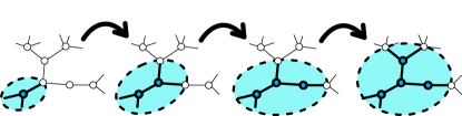
Figure 4: Greedy Expansion.

To find the local optimum in each iteration, the greedy expansion needs to calculate the objective function (Eq. (1) in Def. 4) for partial ordered edges, $X^{\phi}$($\subseteq E^{\phi}$). However, Eq. (1) is defined only for the entire edges (i.e., $E^{\phi}$) and cannot be computed for $X^{\phi}$. Thus, we modify the summation over $p$ (i.e., $\sum_{p}$) in Eq. (1) into one over $E$ (i.e., $\sum_{E}$) so that the algorithm can evaluate $X^{\phi}$ in each iteration.

To do so, we additionally define a function $S$ that detects candidates for the splitting points when the edges will be partitioned via the chunk-based edge partitioning. Based on $S$, Eq. (1) is modified into an summation over $E$ (i.e., $\sum_{E}$).

Definition 5 (Graph Edge Ordering II)

Suppose

$$f_{k}(i,w):=\displaystyle S_{k}(i)\cdot\left|V\left(E^{\phi}_{ch}\left(i-w+1,w\right)\right)\right|,$$

$$S_{k}(i):=\begin{cases}1\ \text{ if }\texttt{ID2P}_{k}(i)\not=\texttt{ID2P}_{k}(i+1)\text{ or }i=|E|-1\\ 0\ \text{otherwise}\end{cases}$$

where we extend the definition of the edge chunk such that $E^{\phi}_{ch}(i^{\prime},w):=E^{\phi}_{ch}(0,w)$ for $i^{\prime}<0$.

Then, the objective of the graph edge ordering problem is redefined as follows:

$$\min_{\phi\in\Phi}\frac{1}{|V|}\sum_{k=k_{\mathit{min}}}^{k_{\mathit{max}}}\sum_{i=0}^{|E|-1}f_{k}\left(i,\left\lfloor\tfrac{|E|+\texttt{ID2P}_{k}(i)}{k}\right\rfloor\right).$$ (6)

The following gives the correctness of the modification.

Lemma 1

Definition 4 and 5 are equivalent.

Proof

In Eq. (6), according to the definition of $S_{k}(i)$,
$f_{k}\left(i,\left\lfloor\tfrac{|E|+\texttt{ID2P}_{k}(i)}{k}\right\rfloor\right)$ is non-zero only if

$$i=\left\lfloor\tfrac{|E|}{k}\right\rfloor-1,\left\lfloor\tfrac{|E|}{k}\right\rfloor+\left\lfloor\tfrac{|E|+1}{k}\right\rfloor-1,...,\sum_{x=0}^{k-1}\left\lfloor\tfrac{|E|+x}{k}\right\rfloor-1$$

Therefore,

$$\displaystyle\sum_{k=k_{\mathit{min}}}^{k_{\mathit{max}}}\sum_{i=0}^{|E|-1}f_{k}\left(i,\left\lfloor\tfrac{|E|+\texttt{ID2P}_{k}(i)}{k}\right\rfloor\right)$$

$$= \displaystyle\sum_{k=k_{\mathit{min}}}^{k_{\mathit{max}}}\sum_{p=0}^{k-1}f_{k}\left(\sum_{x=0}^{p}\left\lfloor\tfrac{|E|+x}{k}\right\rfloor-1,\left\lfloor\tfrac{|E|+p}{k}\right\rfloor\right)$$

$$= \displaystyle\sum_{k=k_{\mathit{min}}}^{k_{\mathit{max}}}\sum_{p=0}^{k-1}\left|V\left(E^{\phi}_{ch}\left(\sum_{x=0}^{p-1}\left\lfloor\tfrac{|E|+x}{k}\right\rfloor,\left\lfloor\tfrac{|E|+p}{k}\right\rfloor\right)\right)\right|,$$

which is equal to Eq. (1). Therefore, Def. 4 and Def. 5 are equivalent. ∎

Then, we extend the objective function in Def. 5 for the partial ordered edges, $X^{\phi}$($\subseteq E^{\phi}$), as follows:

$$\displaystyle\frac{1}{|V|}\sum_{k=k_{\mathit{min}}}^{k_{\mathit{max}}}\sum_{i=0}^{|E|-1}f_{k}\left(X^{\phi},i,\left\lfloor\tfrac{|E|+\texttt{ID2P}_{k}(i)}{k}\right\rfloor\right),$$ (7)

where

$$f_{k}\left(X^{\phi},i,w\right):=S_{k}(i)\cdot\left|V\left(X^{\phi}_{ch}\left(i-w+1,w\right)\right)\right|,$$

$$\mathit{X^{\phi}_{\mathit{ch}}}\left(i-w+1,w\right):=\left\{X^{\phi}\left[i-w+1\right],...,X^{\phi}[i]\right\}.$$

Note that for $x\geq|X^{\phi}|$, $X^{\phi}[x]$ does not exist. These cases are defined as follows:

$$\scriptstyle\mathit{X^{\phi}_{\mathit{ch}}}(i-w+1,w):=\begin{cases}\scriptstyle\{X^{\phi}[i-w+1],...,X^{\phi}[|X^{\phi}|-1]\}&\scriptstyle(i-w+1<|X^{\phi}|\leq i)\\ \scriptstyle\varnothing&\scriptstyle(|X^{\phi}|\leq i-w+1)\end{cases}$$

In the remaining of this section, we first propose a baseline algorithm straightforwardly derived from Def. 5. Then, we propose an efficient algorithm for larger graphs, that provides the equivalent ordering result to the baseline’s one but is significantly faster.

4.1 Baseline Greedy Algorithm

Algorithm 2 shows the baseline greedy algorithm. The algorithm involves two main parts: greedy search and ordering. Each vertex is greedily selected in Lines 2–2. Then, its one-hop and two-hop neighbors are processed and appended to $X^{\phi}$ in Lines 2–2.

In the greedy search (Lines 2–2), the objective function (Eq. (7)) is calculated for every frontier vertex in the already ordered part (i.e., $V_{\mathit{rest}}\cap V(X^{\phi})$), and then, a vertex which minimizes Eq. (7), $v_{\mathit{min}}$, is selected.

In the ordering part (Lines 2–2), the algorithm orders all of the $v_{\mathit{min}}$’s one-hop-neighbor edges. Moreover, let $\delta$ be the range of two-hop-neighbor edges to be considered. A two-hop-neighbor edge of $v_{\mathit{min}}$ is considered for ordering if its destination, $w$, is involved in $V(X^{\phi}_{\mathit{ch}}(|X^{\phi}|-\delta,\delta))$. Each neighbor edge is accessed in ascending order of the destination vertex id (we use the default vertex id of each dataset). The reason why such a two-hop neighbor may improve partitioning quality is due to the well-known property that: if vertex $v$ and $u$ are included in partition $P$, then the vertex replications do not increase by adding $e_{v,u}$ to $P$. It is commonly used in the existing methods joseph2012powergraph ; Bourse:2014:BGE:2623330.2623660 ; Petroni:2015:HSP:2806416.2806424 ; Chen:2015:PDG:2741948.2741970 ; Zhang:2017:GEP:3097983.3098033 ; hanai2019distributed .

For $\delta$, we choose the size of the smallest chunk (i.e., $\delta=10^{0}\times\frac{|E|}{k_{\mathit{max}}}$) to maximize both the quality and performance as preliminary evaluated in Figure 5 (Replication Factor is the average value for $k=4,8,16,32,64,128$. $k_{max}=128$.).

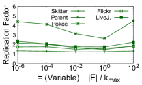
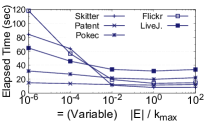
Figure 5: Quality and Performance for Different $\delta$.

Input: $G(V,E)$ – Graph

Output: $X^{\phi}$ – Ordered Edge List

1

2$X^{\phi}$ $\leftarrow$ $\varnothing$; $i$ $\leftarrow$ $0$; $V_{\mathit{rest}}$ $\leftarrow$ $V$

3

4while $|V_{\mathit{rest}}|$ $\not=$ $0$ do

5       /* Greedy Search From Frontier Vertices */

6       $v_{\mathit{min}}$ $\leftarrow$ $\varnothing$; $F_{\mathit{min}}$ $\leftarrow$ $\infty$

7       if $V_{\mathit{rest}}\cap V(X^{\phi})=\varnothing$ then

8             $v_{\mathit{min}}$ $\leftarrow$ $V_{\mathit{rest}}$.RandomVertex()

9            

10      else

11             for $v\in V_{\mathit{rest}}\cap V(X^{\phi})$ do

12                   $X^{\prime\phi}$ $\leftarrow$ $X^{\phi}$ + $\left(N(v)\setminus X^{\phi}\right)$

13                   $F_{v}$ $\leftarrow$ $\displaystyle\tfrac{1}{|V|}\sum_{k=k_{\mathit{min}}}^{k_{\mathit{max}}}\sum_{i=0}^{|E|-1}\scriptstyle f_{k}\left(X^{\prime\phi},i,\left\lfloor\tfrac{|E|+\texttt{ID2P}_{k}(i)}{k}\right\rfloor\right)$

14                   if $F_{v}$ $<$ $F_{\mathit{min}}$ then  $F_{\mathit{min}}$ $\leftarrow$ $F_{v}$; $v_{\mathit{min}}$ $\leftarrow$ $v$

15                  

16            

17      

18      /* Assign New Edge Order */

19       for $e_{v_{\mathit{min}},u}\in N(v_{\mathit{min}})\setminus X^{\phi}$ do

20             $X^{\phi}[i]$ $\leftarrow$ $e_{v_{\mathit{min}},u}$; $i$ $\leftarrow$ $i+1$

21            

22            for $e_{u,w}\in N(u)\setminus X^{\phi}$ do

23                   if $w\in V(X^{\phi}_{\mathit{ch}}(|X^{\phi}|-\delta,\delta))$ then

24                         $X^{\phi}[i]$ $\leftarrow$ $e_{u,w}$; $i$ $\leftarrow$ $i+1$

25                        

26                  

27            

28      

29      $V_{\mathit{rest}}$ $\leftarrow$ $V_{\mathit{rest}}\setminus\{v_{\mathit{min}}\}$

30      

31return $X^{\phi}$

Algorithm 2 Baseline Greedy Algorithm

Theorem 4.1 (Efficiency of Baseline Algorithm)

Efficiency of Algorithm 2 is $O\left(\tfrac{k^{2}_{\mathit{max}}|E|^{2}\cdot|V|^{2}}{k_{\mathit{min}}}\right)$, where $k_{\mathit{max}}$ is much larger than $k_{\mathit{min}}$ s.t. $k_{\mathit{max}}-k_{\mathit{min}}\approx k_{\mathit{max}}$.

Proof

The outermost loop (Lines 2–2) computes $O(|V|)$ iterations. In each iteration, the inner loop from Line 2 to 2 also computes $O(|V|)$ iterations. Moreover, at Line 2, the summation requires $O(|E|\cdot(k_{\mathit{max}}-k_{\mathit{min}}))$ while $f_{k}\left(X^{\phi},i,\tfrac{|E|}{k}\right)$ requires $O\left(\tfrac{k_{\mathit{max}}|E|}{k_{\mathit{min}}}\right)$. Therefore, in total, it requires
$O\left(\tfrac{|V|^{2}\cdot|E|(k_{\mathit{max}}-k_{\mathit{min}})\cdot k_{\mathit{max}}|E|}{k_{\mathit{min}}}\right)=O\left(\tfrac{k^{2}_{\mathit{max}}|E|^{2}\cdot|V|^{2}}{k_{\mathit{min}}}\right)$ under the assumption that $k_{\mathit{max}}-k_{\mathit{min}}\approx k_{\mathit{max}}$. ∎

Input: $G(V,E)$ – Graph

Output: $X^{\phi}$ – Ordered Edge List

1

2$X^{\phi}$ $\leftarrow$ $\varnothing$; $i$ $\leftarrow$ $0$; $V_{\mathit{rest}}$ $\leftarrow$ $V$; $\mathit{PQ}$ $\leftarrow$ $\varnothing$

3 $D[v]$ $\leftarrow$ $|N(v)|$, $M[v]$ $\leftarrow$ $0$ for each $v\in V$

4

5while $|V_{\mathit{rest}}|$ $\not=$ $0$ do

6       $v_{\mathit{min}}$ $\leftarrow$ $\varnothing$

7       if $\mathit{PQ}=\varnothing$ then  $v_{\mathit{min}}$ $\leftarrow$ $V_{\mathit{rest}}$.RandomVertex()

8      else  $v_{\mathit{min}}$ $\leftarrow$ $\mathit{PQ}$.dequeue()

9      

10      for $e_{v_{\mathit{min}},u}\in N(v_{\mathit{min}})\setminus X^{\phi}$ do

11             $X^{\phi}[i]$ $\leftarrow$ $e_{v_{\mathit{min}},u}$; $i$ $\leftarrow$ $i+1$

12             $D[u]$ $\leftarrow$ $D[u]-1$; $M[u]$ $\leftarrow$ $i$

13            

14            for $e_{u,w}\in N(u)\setminus X^{\phi}$ do

15                   if $w\in V(X^{\phi}_{\mathit{ch}}(|X^{\phi}|-\delta,\delta))$ then

16                         $X^{\phi}[i]$ $\leftarrow$ $e_{u,w}$; $i$ $\leftarrow$ $i+1$

17                         $D[u]$ $\leftarrow$ $D[u]-1$; $D[w]$ $\leftarrow$ $D[w]-1$

18                         $M[w]$ $\leftarrow$ $i$; $M[u]$ $\leftarrow$ $i$

19                         $\mathit{PQ}$.update($D[w]$,$M[w]$,$w$)

20                        

21                  

22            

23            if $u\not\in\mathit{PQ}$ then  $\mathit{PQ}$.enqueue($D[u]$,$M[u]$,$u$)

24            else  $\mathit{PQ}$.update($D[u]$,$M[u]$,$u$)

25            

26      

27      $V_{\mathit{rest}}$ $\leftarrow$ $V_{\mathit{rest}}\setminus\{v_{\mathit{min}}\}$

28      

29return $X^{\phi}$

Algorithm 3 PQ-based Fast Algorithm

4.2 Fast Algorithm Based on Priority Queue

We propose an efficient greedy algorithm based on the priority queue, which provides the equivalent result to the baseline algorithm (Algorithm 2). Although Algorithm 2 provides an approximate solution of the NP-hard problem, its computational cost (Theorem 4.1) is still high as the real-world graph is typically large, including billions of elements.

Algorithm 3 shows the efficient algorithm. Overall, its computation is the same as Algorithm 2, which begins with a random vertex. Then, the algorithm iteratively and greedily expands the ordered parts until all the edges are ordered.

The key difference from Algorithm 2 is that Algorithm 3 utilizes a priority queue, $\mathit{PQ}$, to evaluate the objective function (Eq. (7)) instead of calculating the equation for every frontier vertex in $V_{\mathit{rest}}\cap V(X^{\phi})$. Specifically, $\mathit{PQ}$ uses a priority represented as follows:

$$p(v):=\alpha\cdot D[v]-\beta\cdot M[v],$$ (8)

where $\alpha:=\sum_{k=k_{\mathit{min}}}^{k_{\mathit{max}}}\left\lfloor\tfrac{|E|}{k}\right\rfloor$ and $\beta:=k_{\mathit{max}}-k_{\mathit{min}}$ are computed in advance of the greedy expansion. The frontier vertices are sorted in the ascending order by $p$. $D[v]$ $(v\in V)$ is the $v$’s degrees for the rest of the edges (i.e., $D[v]:=|N(v)\setminus X^{\phi}|$). $M[v]$ stores the latest order of an edge which involves $v$. $M[v]$ is updated each time a new edge order is assigned (Line 3 and Line 3 in Algorithm 3).

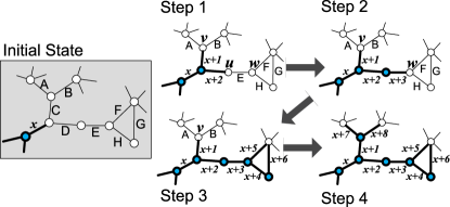
Figure 6: Greedy Expansion in Fast Algorithm. Edge A,B,..,H is ordered into $x+1,x+2,...x+8$.

Figure 6 shows an example of the greedy expansion. After assigning the order to Edge C and Edge D, two frontier vertices, $v$ and $u$, exist in the graph. The algorithm selects $u$ and assigns $x+3$ to Edge E because $p(u)<p(v)$. Then, $v$ and $w$ become the frontier. Then, $w$ is selected because $p(w)<p(v)$. The algorithm assigns $x+4$, $x+5$, $x+6$ to Edge F, H, G, respectively. Finally, $v$ is selected. Then, Edge A and B are ordered to $x+7$ and $x+8$, respectively.

The equivalence of Algorithm 2 and Algorithm 3 is established by the following lemma. It shows that the calculation of Eq. (7) can be replaced into $PQ$ based on $p$ (Eq. (8)):

Lemma 2

Suppose $|E|$ is much larger than $k_{max}$ such that $w:=\left\lfloor\tfrac{|E|}{k}\right\rfloor=\left\lfloor\tfrac{|E|+\texttt{ID2P}_{k}(\cdot)}{k}\right\rfloor$ and $D[v]<\tfrac{|E|}{k_{max}}$ for $\forall v\in V$.

Then, $\forall v,u\in V_{\mathit{rest}}\cap V(X^{\phi})$,   $p(v)>p(u)\Rightarrow F_{v}>F_{u}$, where $F_{v}$ and $F_{u}$ are the value of Eq. (7) for $X^{\phi}+N(v)$ and $X^{\phi}+N(u)$ respectively, as shown in Line 2 of Algorithm 2.

Proof

Suppose $\mathit{Xv}^{\phi}:=X^{\phi}+N(v)$, $\mathit{Xu}^{\phi}:=X^{\phi}+N(u)$.

$$F_{v}>F_{u}\ \ \Leftrightarrow\ \ F_{v}-F_{u}>0$$ (9)

$$\Leftrightarrow \displaystyle\sum_{k=k_{\mathit{min}}}^{k_{\mathit{max}}}\sum_{i=0}^{|E|-1}\left\{f\left(\mathit{Xv}^{\phi},i,w\right)-f\left(\mathit{Xu}^{\phi},i,w\right)\right\}{\displaystyle>0}$$

$$\Leftarrow \displaystyle\sum_{k=k_{\mathit{min}}}^{k_{\mathit{max}}}\sum_{i=0}^{|E|-1}\scriptstyle\left\{\left|V\left(\mathit{Xv}^{\phi}_{ch}\left(i-w+1,w\right)\right)\right|-\left|V\left(\mathit{Xu}^{\phi}_{ch}\left(i-w+1,w\right)\right)\right|\right\}$$

$${\displaystyle>0}$$

$$\Leftrightarrow \displaystyle\displaystyle\sum_{k=k_{\mathit{min}}}^{k_{\mathit{max}}}\sum_{i=|X|^{\phi}}^{|E|-1}\left\{\Delta V(v,i)-\Delta V(u,i)\right\}>0,$$

where $\Delta V(v,i):=|V(\mathit{Xv}^{\phi}_{ch}(\scriptstyle{i-w+1,w}\displaystyle))|-|V(X^{\phi}_{ch}(\scriptstyle{i-w+1,w}\displaystyle))|$.

Next, we will calculate $\Delta V(v,i)$ for $i\geq|X^{\phi}|$. Intuitively, $\Delta V(v,i)$ means the number of additional replicated vertices in a chunk when we select $v$ to expand the ordered edges. For each chunk determined by $i$, each additional replicated vertex comes from $v$ or $N(v)$. Thus, $\Delta V(v,i)$ can be represented by the sum of two functions:

$$\Delta V(v,i)=\chi(i)+n(i),$$

where $\chi(i)$ is the number of replicated vertices caused by $v$; $n(i)$ is caused by $N(v)$.

First, $\chi(i)$ is the indicator function. If $X^{\phi}_{ch}(i-w+1,w)$ already involves $v$, then the number of replicated vertices does not increase due to the additional $v$. Therefore, $\chi(i)$ is 0. Specifically, this case appears if $i>M[v]+w$, because $X^{\phi}_{ch}(i-w+1,w)$ involves an edge $e$ whose order is $M[v]$ (i.e., $\phi(e)=M[v]$). Otherwise, $v$’s replication is newly added to the chunk $Xv^{\phi}_{ch}(i-w+1,w)$, and thus $\chi(i)$ is 1. Therefore, $\chi(i)$ is represented as follows:

$$\chi(i)=\begin{cases}1&\text{if }i\in[M[v]+w,|X^{\phi}|+D[v]+w)\\ 0&\text{if }i\not\in[M[v]+w,|X^{\phi}|+D[v]+w)\end{cases}$$

where we also consider a case that $i$ is larger so that $Xv^{\phi}_{ch}(i-w+1,w)$ is empty. In this case, $\chi(i)$ is obviously 0.

Second, $n(i)$ is the number of the additional vertices derived from $N(v)$. Its value can be represented as follows:

$$n(i)=\begin{cases}i-|X^{\phi}|&(|X^{\phi}|\leq i<|X^{\phi}|+D[v])\\ D[v]&(|X^{\phi}|+D[v]\leq i<|X^{\phi}|+w)\\ \scriptstyle D[v]-i+|X^{\phi}|+w&(|X^{\phi}|+w\leq i<|X^{\phi}|+D[v]+w)\\ 0&(|X^{\phi}|+D[v]+w<i)\\ \end{cases}$$

Figure 7 shows an example of these cases. Suppose $v$ is selected in the greedy algorithm and new edge orders are assigned to $v$’s neighbor edges, $e_{v,u_{0}}$, $e_{v,u_{1}}$, $e_{v,u_{2}}$, $e_{v,u_{3}}$, and $e_{v,u_{4}}$. Then, if $|X^{\phi}|\leq i<|X^{\phi}|+D[v]$, a part of $N(v)$ are added (e.g., $u_{0},u_{1},u_{2}$ in Figure 7). If $|X^{\phi}|+D[v]\leq i<|X^{\phi}|+w$, all vertices in $N(v)$ are added (e.g., $u_{0},u_{1},u_{2},u_{3},u_{4}$ in Figure 7). If $|X^{\phi}|+w\leq i<|X^{\phi}|+D[v]+w$, also a part of $N(v)$ are added (e.g., $u_{2},u_{3},u_{4}$ in Figure 7). If $|X^{\phi}|+D[v]+w\leq i$, then $Xv^{\phi}_{ch}(i-w+1,w)$ involves no vertices.

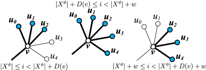
Figure 7: The value of $n(i)$: # of the additional vertices derived from $N(v)=\{u_{0},u_{1},...,u_{4}\}$. Blue vertices are the additional when $v$ is selected for the expansion.

Therefore,

$$\displaystyle\sum_{\mathclap{i=|X^{\phi}|}}^{\mathclap{|E|-1}}\Delta V(v,i)= \displaystyle\sum_{\mathclap{i=|X^{\phi}|}}^{\mathclap{|E|-1}}\chi(i)+\ \ \sum_{\mathclap{i=|X^{\phi}|}}^{\mathclap{|X^{\phi}|+D[v]-1}}\left\{i-|X^{\phi}|\right\}\ +\ \sum_{\mathclap{i=|X^{\phi}|+D[v]}}^{\mathclap{|X^{\phi}|+w-1}}D[v]$$

$$\displaystyle+\sum_{\mathclap{i=|X^{\phi}|+w}}^{\mathclap{|X^{\phi}|+w+D[v]-1}}\left\{D[v]-i+|X^{\phi}|+w\right\}$$

$$= wD[v]+|X^{\phi}|+D[v]-M[v]$$

Let $\Delta D:=D[v]-D[u]$ and $\Delta M:=M[v]-M[u]$.

$$\displaystyle\sum_{\mathclap{i=|X^{\phi}|}}^{\mathclap{|E|-1}}\left\{\Delta V(v,i)-\Delta V(u,i)\right\}=w\Delta D+\Delta D-\Delta M$$

$$\sim w\Delta D-\Delta M\ \ (\because w>\tfrac{|E|}{k_{max}}\gg 1)$$

Therefore,

$$p(v)>p(u)$$

$$\Leftrightarrow \alpha\cdot D[v]-\beta\cdot M[v]>\alpha\cdot D[u]-\beta\cdot M[u]$$

$$\Leftrightarrow \sum_{k=k_{min}}^{k_{max}}\left(w\cdot D[v]-M[v]\right)>\sum_{k=k_{min}}^{k_{max}}\left(w\cdot D[u]-M[u]\right)$$

$$\Leftrightarrow \sum_{k=k_{min}}^{k_{max}}\left(w\Delta D-\Delta M\right)>0$$

$$\Leftrightarrow \displaystyle\sum_{k=k_{min}}^{k_{max}}\sum_{i=|X^{\phi}|}^{|E|-1}\left\{\Delta V(v,i)-\Delta V(u,i)\right\}>0$$

$$\Rightarrow F_{v}>F_{u}.\ \ \ (\because\eqref{eq:ff})$$

Thus, the lemma is proved. ∎

Algorithm 3 significantly reduces the time complexity.

Theorem 4.2 (Efficiency of Fast Algorithm)

Suppose $\mathit{PQ}$ be a standard priority-queue implementation, where dequeue, update or enqueue can be operated in $O(\log n)$. Then, time complexity of Algorithm 3 is
$O(d_{\mathit{max}}^{2}|V|\log|V|)$, where $d_{\mathit{max}}$ is the maximum degree.

Proof

The outermost loop (Lines 3 – 3) requires $O(|V|)$ for each vertex. Then, the inner loop (Lines 3 – 3) needs $O(d_{\mathit{max}})$ for each neighbors of $v_{\mathit{min}}$. Finally, the innermost loop (Lines 3 – 3) requires $O(d_{\mathit{max}})$ for each neighbors and $O(\log|V|)$ for updating $PQ$ at Line 3. To sum up, the total time complexity of Algorithm 3 is $O(d_{\mathit{max}}^{2}|V|\log|V|)$. ∎

5 Theoretical Analysis

In this section, we provide a theoretical analysis for the upper bound of the partitioning quality achieved by our method. Our analysis focuses on the observation that in typical practical situations, the minimum partition size is much larger than the maximum degree of the graph. In this case, the number of new ordered edges in each iteration of Algorithm 3 becomes smaller than the smallest partition size. Based on this fact, we formulate the following theorem.

Theorem 5.1 (Upper Bound of Partitioning Quality)

Consider that in each iteration of Algorithm 3 (Lines 3–3) the number of new ordered edges is smaller than the smallest partition size and that $\delta=\left\lfloor\frac{|E|}{k_{max}}\right\rfloor-1$.

Let $E$ be ordered by Algorithm 3 and then partitioned into $k$ parts, $\mathcal{E}_{k}$, via chunk-based partitioning. Then, the replication factor, $RF_{k}$, for the $k$ edge partitions has an upper bound as follows:

$$RF_{k}:=\sum_{p=0}^{k-1}\frac{|V(\mathcal{E}_{k}[p])|}{|V|}\leq\frac{|V|+|E|+k}{|V|}$$

Proof

Assume that $k$ is given in advance. We consider a new partitioning algorithm based on the ordering algorithm (Algorithm 3) and conversion function $\texttt{ID2P}_{k}(i)$ (Algorithm 1) as follows:

• Initially, the $k$ edge partitions, $\mathcal{E}_{k}$, are empty.

• Run Algorithm 3 and insert $i$-th ordered edge
  to $\mathcal{E}_{k}[\texttt{ID2P}_{k}(i)]$.

In the new partitioning algorithm, the edge partitions are incrementally determined from $\mathcal{E}_{k}[0]$, $\mathcal{E}_{k}[1]$, …, to $\mathcal{E}_{k}[k-1]$. Obviously, the partitioning results obtained by the new partitioning algorithm is the same as the ones by our proposed method (i.e., completing Algorithm 3 before the chunk-based edge partitioning for $k$.)

Let $t$ be an iteration counter for Lines 3–3 of Algorithm 3, and $\Phi(t)$ be a potential function over $t$ defined as follows:

$$\Phi(t):=|V_{rest}(t)|+|E_{rest}(t)|+p_{rest}(t)+\sum_{p=0}^{k-1}|V(\mathcal{E}_{k}(t)[p])|,$$

where $V_{rest}(t)$ is a set of vertices adjacent to at least one non-ordered edge; $E_{rest}(t)$ is a set of non-ordered edges at $t$; $p_{rest}(t)$ is the number of partitions which still have spaces to insert edges; $\mathcal{E}_{k}(t)$ is a set of edge partitions at $t$.

Suppose the ordering algorithm terminates at $T$. We will show that (a) $\Phi(0)=|V|+|E|+k$, (b) $\Phi(T)=\sum_{p=0}^{k-1}V(\mathcal{E}_{k}[p])$, and (c) $\Phi(0)\geq\Phi(T)$. The first two equations (a) and (b) are obvious, i.e.,

$$\Phi(0) :=|V_{rest}(0)|+|E_{rest}(0)|$$

$$\ \ \ \ \ \ \ \ +p_{rest}(0)+\sum_{p=0}^{k-1}|V(\mathcal{E}_{k}(0)[p])|$$

$$=|V|+|E|+k$$

$$\Phi(T) :=|V_{rest}(T)|+|E_{rest}(T)|$$

$$\ \ \ \ \ \ \ \ +p_{rest}(T)+\sum_{p=0}^{k-1}|V(\mathcal{E}_{k}(T)[p])|$$

$$=\sum_{p=0}^{k-1}|V(\mathcal{E}_{k}[p])|$$

For (c), we will show $\Phi(t)-\Phi(t-1)\geq 0$ for $0<t\leq T$. Let $\Delta\Phi:=\Phi(t)-\Phi(t-1)$, $\Delta V_{rest}:=|V_{rest}(t)|-|V_{rest}(t-1)|$, $\Delta E_{rest}:=|E_{rest}(t)|-|E_{rest}(t-1)|$, $\Delta p_{rest}:=p_{rest}(t)-p_{rest}(t-1)$, and $\Delta V(\mathcal{E}):=\sum_{p=0}^{k-1}|V(\mathcal{E}_{k}(t)[p])|-\sum_{p=0}^{k-1}|V(\mathcal{E}_{k}(t-1)[p])|$.

For $t$-th iteration where $v_{min}$ is selected for expansion, we define the number of $v_{min}$’s one-hop neighbor edges which are ordered at $t$ as $n_{one}$ and the number of $v_{min}$’s two-hop neighbor edges which are ordered at $t$ as $n_{two}$. For example in Figure 8, $v_{min}$ is selected and the edges are ordered from $x$ to $x+9$. Here, $n_{one}=3$ (Edges $x$, $x+5$, $x+9$) and $n_{two}=7$ (Edges $x+1,x+2,x+3,x+4,x+6,x+7,x+8$).

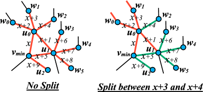
Figure 8: One Iteration for Ordering.

Then, $\Delta V_{rest}\leq-1$ because all of $v_{min}$’s neighbor edges are assigned at the iteration. $\Delta E_{rest}=-(n_{one}+n_{two})$ from the definition.

$\Delta p_{rest}=0$ if all the ordered edges during the iteration are inserted to the same partition as the previous iteration and the partition has still have free space (Case A). Otherwise (Case B), i.e., if the partitioning set becomes full during the current iteration, then $\Delta p_{rest}=-1$. Note that during an iteration of the algorithm, there cannot be more than one partitioning set that becomes full due to the assumption that the number of new assigned edges in each iteration is smaller than the smallest partition size.

For $\Delta V(\mathcal{E})$, we consider Case A and B as well. In Case A, $\Delta V(\mathcal{E})\leq 1+n_{one}+n_{two}$ because $v_{min}$ may be newly inserted; $n_{one}$ vertices and up to $n_{two}$ vertices may be to the current partition. For example in Figure 8, $u_{i}(i=0,1,2)$ are newly inserted as $n_{one}$ and $w_{i}(i=0,..,5)$ are as $n_{two}-1(\leq n_{two})$.

In Case B, $\Delta V(\mathcal{E})$ satisfies the following equation:

$$\Delta V(\mathcal{E})\leq 2+(n_{one}+2)+(n_{two}-2).$$ (10)

As explained above in Case B, there cannot be more than one partitioning set that becomes full. This is translated into having up to two partitions at an iteration. Thus, let the two partitions be $\mathcal{E}_{k}[p_{0}]$ and $\mathcal{E}_{k}[p_{1}]$, where each edge is inserted to $\mathcal{E}_{k}[p_{0}]$ at first and then $\mathcal{E}_{k}[p_{1}]$ after splitting.

The first “$2$” in Eq.(10) means that $v_{min}$ may be inserted to up to two partitions ($\mathcal{E}_{k}[p_{0}]$ and $\mathcal{E}_{k}[p_{1}]$). The second “$(n_{one}+2)$” in Eq.(10) means that $n_{one}$ vertices are inserted to either $\mathcal{E}_{k}[p_{0}]$ or $\mathcal{E}_{k}[p_{1}]$. In addition, up to two of $n_{one}$ vertices may be inserted to both $\mathcal{E}_{k}[p_{0}]$ and $\mathcal{E}_{k}[p_{1}]$. This is because there may be up to two partitions at an iteration.

Let the splitting point be between $i$ and $i+1$. The last “$(n_{two}-2)$” in Eq.(10) means that up to $n_{two}$ vertices are inserted to either $\mathcal{E}_{k}[p_{0}]$ or $\mathcal{E}_{k}[p_{1}]$. But at least the last two edges for $\mathcal{E}_{k}[p_{0}]$ (i.e., $i-1$-th and $i$-th edges) never increase the number of duplicated vertices. This is because the two-hop vertices adjacent to $i-1$-th and $i$-th edges must belong to $\mathcal{E}_{k}[p_{0}]$. The above is proved as follows.

Let the two-hop vertices adjacent to $i-1$-th and $i$-th edges be $w$ and $w^{\prime}$; $X^{\phi}$ be the ordered edges up to $i$-th edge. Note that $w$ and $w^{\prime}$ must be in $V(X^{\phi}_{\mathit{ch}}(i-\delta,\delta))$ and $V(X^{\phi}_{\mathit{ch}}(i+1-\delta,\delta))$ respectively, due to the condition in Line 11 of Algorithm 3. Then, according to the assumption that $\delta=\left\lfloor\frac{|E|}{k_{max}}\right\rfloor-1$, $w$ is in

$$V\left(X^{\phi}_{\mathit{ch}}\left(i-\left(\left\lfloor\frac{|E|}{k_{max}}\right\rfloor-1\right),\left\lfloor\frac{|E|}{k_{max}}\right\rfloor\right)\right)$$

$$=V\left(X^{\phi}_{\mathit{ch}}\left(i+1-\left\lfloor\frac{|E|}{k_{max}}\right\rfloor,\left\lfloor\frac{|E|}{k_{max}}\right\rfloor\right)\right)$$

$$\subseteq V\left(X^{\phi}_{\mathit{ch}}\left(i+1-\left\lfloor\frac{|E|+p_{0}}{k_{max}}\right\rfloor,\left\lfloor\frac{|E|+p_{0}}{k_{max}}\right\rfloor\right)\right)$$

$$\subseteq V\left(X^{\phi}_{\mathit{ch}}\left(i+1-\left\lfloor\frac{|E|+p_{0}}{k}\right\rfloor,\left\lfloor\frac{|E|+p_{0}}{k}\right\rfloor\right)\right)$$

$$=V(\mathcal{E}_{k}[p_{0}])$$

Similarly, $w^{\prime}$ is also in $V(\mathcal{E}_{k}[p_{0}])$.

For example in Figure 8, the ordered edges are split between $x+3$ and $x+4$ ($\mathcal{E}_{k}[p_{0}]$ is red. $\mathcal{E}_{k}[p_{1}]$ is green). In this case, $v_{min}$ is inserted to both $\mathcal{E}_{k}[p_{0}]$ and $\mathcal{E}_{k}[p_{1}]$. $u_{0}$ and $u_{1}$ are also inserted to both, but $u_{2}$ is inserted only to $\mathcal{E}_{k}[p_{1}]$. $w_{0}$–$w_{5}$ are inserted to either $\mathcal{E}_{k}[p_{0}]$ or $\mathcal{E}_{k}[p_{1}]$, but $w_{0}$ and $w_{1}$ are not duplicated because they include edges which have already been assigned to $\mathcal{E}_{k}[p_{0}]$. Thus, in total, $\Delta V(\mathcal{E})=2+2+2+1+4=11$, which is smaller than $2+(n_{one}+2)+(n_{two}-2)=12$.

Then, to summarize the above discussion, $\Delta\Phi$ can be calculated as follows:

$$\Delta\Phi=\Delta V_{rest}+\Delta E_{rest}+\Delta p_{rest}+\Delta V(\mathcal{E})$$

$$\leq\begin{cases}\scriptstyle-1-(n_{one}+n_{two})+0+1+n_{one}+n_{two}\ (\text{Case A})\\ \scriptstyle-1-(n_{one}+n_{two})-1+2+(n_{one}+2)+(n_{two}-2)\ (\text{Case B})\end{cases}$$

$$=0$$

Therefore, $\Delta\Phi\leq 0$ and thus (c) hold.

Based on (a), (b), (c), we establish the following equation:

$$RF_{k} :=\sum_{p=0}^{k-1}\frac{|V(\mathcal{E}_{k}[p])|}{|V|}=\frac{\Phi(T)}{|V|}\leq\frac{\Phi(0)}{|V|}=\frac{|V|+|E|+k}{|V|}$$

Finally, the theorem is proved. ∎

Comparison to Existing Upper Bounds. We compare our upper bound to the existing edge partitioning methods. Our method provides an upper bound for general graphs, but most of the existing methods provide an upper bound only for power-law graphs. Thus, we apply our upper bound to the power-law graph.

By using Clauset’s power-law model clauset2009power , we model a graph, $G_{\zeta}(V,E)$, satisfying the following condition:

$$Pr[d]=d^{-\alpha}\cdot\zeta(d,d_{min})^{-1},$$ (11)

where $Pr[d]$ is the probability that vertex’s degree becomes $d$; $\alpha$ is the scaling parameter (typically, $2<\alpha<3$ for real-world graphs); $\zeta(d,d_{min})$ is the generalized/Hurwitz zeta function; and $d_{min}$ is the minimum degree. We assume that $d_{min}=1$ (then, $\zeta(d,d_{min})$ becomes Riemann zeta function) and that for any $k$, $|V|\gg k$ s.t. $k/|V|\approx 0$.

The expected value of the upper bound for $G_{\zeta}$ is formalized as follows:

$$\mathbb{E}\left[\frac{|V|+|E|+k}{|V|}\right]\approx 1+\mathbb{E}\left[\frac{|E|}{|V|}\right]$$

$$=1+\frac{(G_{\zeta}\text{'s mean degree})}{2}$$

$$=1+\frac{(\text{Mean of Eq.\eqref{eq:degree}},d_{min}=1)}{2}$$

$$=1+\frac{1}{2}\cdot\frac{\zeta(\alpha-1,1)}{\zeta(\alpha,1)},$$

where the last equation is given by the mean value of the zeta distribution.

Table 2 shows the calculation results under various $\alpha$ when $k=256$. We calculate the existing upper bounds based on NIPS2014_5396 ; Petroni:2015:HSP:2806416.2806424 ; Zhang:2017:GEP:3097983.3098033 ; dynamicscaling . NE Zhang:2017:GEP:3097983.3098033 provides the best quality. Our method is the second best and its score is very similar to NE. The quality gap between the top two methods and the other ones is significant especially when $\alpha$ is small (i.e., a graph is more skewed). Also, the small quality difference between our method and NE is due to the fact that our method can be applied with arbitrary $k$ values while NE is restricted with the fixed $k$. Such trends also appear in the empirical result in Sec. 6.

Table 2: Theoretical Upper Bound of Replication Factor in Power-law Graph ($256$ Partition, $|V|=10^{6}$).

Partitioner	$\alpha=$ 2.2	2.4	2.6	2.8
Random (1D-hash)	5.88	3.46	2.64	2.23
Grid (2D-hash)	4.82	3.13	2.47	2.13
DBH NIPS2014_5396	5.59	3.21	2.43	2.05
HDRF Petroni:2015:HSP:2806416.2806424	5.36	4.23	3.61	3.24
NE Zhang:2017:GEP:3097983.3098033	2.81	1.68	1.31	1.13
BVC dynamicscaling	11.10	6.39	4.85	4.10
Proposed Method	2.88	2.12	1.88	1.75

6 Evaluation

In this section, we provide a comprehensive evaluation of our two proposed methods: the graph edge ordering and the chunk-based edge partitioning.

Our main results are summarized as follows:

Highest Scaling Efficiency. The chunk-based edge partitioning is significantly faster than the existing methods. Even compared to the very efficient simple hashing method, the chunk-based edge partitioning is over three orders of magnitude faster.

Similar Partitioning Quality to the Best Graph Partitioning Method. The quality of edge partitions that the graph edge ordering and the chunk-based edge partitioning generate is comparable to the high-quality but time-consuming $k$-way graph partitioning methods. The quality-loss due to variable $k$ in our method is small.

Highest Partitioning Quality Compared to Graph Ordering Methods. Among the existing ordering methods, the graph edge ordering delivers the best improvement to the partitioning quality of the chunk-based edge partitioning.

Acceptable Preprocessing Time. Due to the efficient greedy algorithm, the elapsed time for the graph edge ordering is similar to the other ordering methods. It can order billion-edge graphs within an acceptable time.

Performance Improvement in Distributed Graph Applications. Edge partitions generated by the chunk-based edge partitioning and the graph edge ordering highly improve the performance of the distributed graph applications (SSSP, WCC, and PageRank) due to the large reduction of communication volumes.

Moreover, the evaluation result for the migration cost and the scalability of our proposed algorithm are shown as additional experiments.

6.1 Experimental Frame

Graph Data Sets. We use various types of real-world large graphs (over 1 million vertices) provided by SNAP snapnets and KONNECT KONECT as summarized in Table 3. Road-CA is the road network of California. Skitter is the internet topology graph of autonomous systems. Patents is the citation network. Pokec, Flickr, LiveJ., Orkut, Twitter, and FriendS. are online social networks in each service. Road-CA is a non-skewed graph, whereas the others are skewed graphs, namely, they have skewed degree distribution.

Table 3: Datasets (M = Million, B = Billion)

Dataset	$|V|$	$|E|$	Type
Road-CA leskovec2009community	1.96 M	2.76 M	Traffic
Skitter leskovec2005graphs	1.70 M	11.09 M	Internet
Patents leskovec2005graphs	3.77 M	16.51 M	Citation
Pokec takac2012data	1.63 M	30.62 M	Social Net.
Flickr Mislove:2008:GFS:1397735.1397742	2.30 M	33.14 M	Social Net.
LiveJ. Backstrom:2006:GFL:1150402.1150412	4.8 M	68 M	Social Net.
Orkut 6413740	3.1 M	117 M	Social Net.
Twitter Kwak:2010:TSN:1772690.1772751	41.6 M	1.46 B	Social Net.
FriendS. yang2012defining	65.6 M	1.80 B	Social Net.

Table 4: Graph Partitioning Methods.

Method	Part by	Description
BVC dynamicscaling	Edge	State-of-the-art dynamic scaling
NE Zhang:2017:GEP:3097983.3098033	Edge	Highest-quality offline method
DBH NIPS2014_5396	Edge	Degree-based hashing method
HDRF Petroni:2015:HSP:2806416.2806424	Edge	High-Degree Replicated First
1D/2D	Edge	1D / 2D random hash
MTS Karypis:1998:FHQ:305219.305248	Vertex	METIS
CVP zhu2016gemini	Vertex	Chunk-based vertex partitioning
CEP	Edge	Chunk-based edge partitioning

Table 5: Graph Ordering Methods

Method	Order by	Description
GO wei2016speedup	Vertex	Optimized to L1-cache
RO arai2016rabbit	Vertex	RabbitOrder
RGB dhulipala2016compressing	Vertex	Recursive Graph Bisection
LLP boldi2011layered	Vertex	Layered Label Propagation
RCM Cuthill:1969:RBS:800195.805928	Vertex	Reverse Cuthill–McKee
DEG	Vertex	Simple degree sorting
DEF	Vertex	Default ordering
GEO	Edge	Proposed Greedy Algorithm

Comparing Methods. We compare our two methods with 15 existing methods, as shown in Table 4 and Table 5. We refer to the chunk-based edge partitioning as CEP, and to the efficient greedy algorithm (i.e., Algorithm 3) for the graph edge ordering as GEO. We classify all the methods into five categories: dynamic scaling, edge/vertex partitioning, and edge/vertex ordering.

Table 4 shows algorithms of the dynamic scaling and graph partitioning. BVC (precisely, BVC^+/-) is the state-of-the-art dynamic scaling method for graph partitions based on consistent hashing. NE is the latest offline edge partitioning method, which basically provides the best-quality edge partitioning in practice. DBH is the degree-based-hashing edge partitioning. HDRF is High-Degree Replicated First streaming edge partitioning. 1D and 2D are simple hash-based edge partitioning. In 1D, each edge is randomly assigned to 1D integer partitioning id space (0,1,2,…) by hashing its edge id. In 2D, each edge is randomly assigned to 2D partitioning id space ($<0,0>$, $<0,1>$,.., $<1,0>$, $<1,1>$, …) by separately hashing its source id and destination id. The hash value of the source id determines the first dimension while that of the destination id does the second dimension.  MTS (METIS) is the high-quality offline vertex partitioning method. CVP is the chunk-based vertex partitioning, where the ordered vertex is simply divided into the same size of vertex chunks. Table 5 shows algorithms of graph ordering. GO and RO are vertex id ordering methods for maximizing CPU-cache utilization. RGB and LLP are for graph compression. DEG is simple degree sorting. DEF is default ordering.

Computational Infrastructure. We use Ubuntu server (ver. 18.04) with dual sockets of Intel Xeon CPU E5-2697 v4 (18 cores per socket, 2.30GHz) and 500GB RAM. All the programs except for LLP and HDRF are written in C/C++, which we compile via GCC 7.4.0 with –O3 optimization flag. For LLP and HDRF, we use OpenJDK version 11.0.4 on 400GB JVM memory. Although some of the algorithms, such as RO or BVC, support the parallel execution, all the programs are run on a single core for a fair comparison. The parallelization of our methods, especially GEO, is an interesting problem but out of scope in this paper. We list it as our future work in Sec. 7.

Parameters. According to the existing experimental studies on distributed graph processing systems and graph partitioning Han:2014:ECP:2732977.2732980 ; 6877273 ; Verma:2017:ECP:3055540.3055543 ; abbas2018streaming ; Gill:2018:SPP:3297753.3316427 ; Pacaci:2019:EAS:3299869.3300076 , the number of distributed processes (i.e., partitions) for graph applications usually ranges from less than 10 to around one hundred. Thus, in the evaluation, we change the number of partitions, $k$, from 4 to 128. For GEO, $k_{min}$ and $k_{max}$, as defined in Def. 4 of Sec. 3.4, are $4$ and $128$, respectively.

6.2 Comparison with Graph Partitioning

We compare our methods to the existing graph partitioning methods and dynamic scaling methods, as shown in Table 4. Note that for 128 partitions, NE and MST cannot correctly execute FriendSter, nor can NE do Twitter. For BVC, we run the algorithm as $k$ is $4\rightarrow 8\rightarrow 16\rightarrow 32\rightarrow 64\rightarrow 128$, and we set the balance factor $\epsilon=0.001$ as defined in Def. 2.

Scaling Efficiency. Efficiency is measured by the elapsed time. Figure 9 shows the elapsed time for each method. In BVC, we measure the repartitioning time from the previous partitions (e.g., for $k=8$, time from $k=4$ to $k=8$ is used.). We ignore the initialization phase, such as, data loading and graph construction, and the graph data migration phase.

As expected, CEP is significantly faster than the others due to its $\mathcal{O}(1)$ time complexity. It is over 1,000 times faster than the other methods for all the data sets. Also, the performance of CEP is not changed with the increase of the graph size, which is a consistent result to Theorem 3.1. In the other existing methods, even for the very simple partitioning, such as 1D/2D or CVP, each edge needs to be processed one-by-one, resulting in that the elapsed time increases proportionally to the graph size.

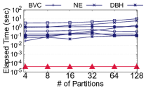
(a) Road-CA

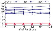
(b) Skitter

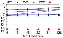
(c) Patent

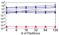
(d) Pokec

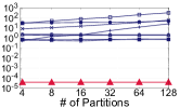
(e) Flickr

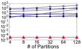
(f) LiveJournal

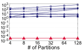
(g) Orkut

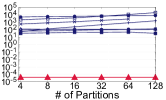
(h) Twitter

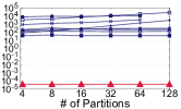
(i) FriendSter

Figure 9: Elapsed Time for Graph Partitioning.

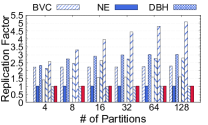
(a) Road-CA

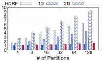
(b) Skitter

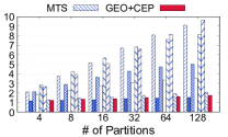
(c) Patent

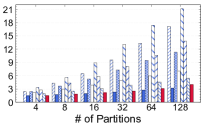
(d) Pokec

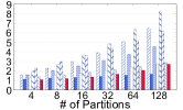
(e) Flickr

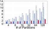
(f) LiveJournal

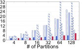
(g) Orkut

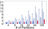
(h) Twitter

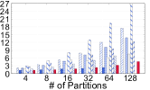
(i) FrindSter

Figure 10: Replication Factor Compared to Graph Partitioning Methods.

Partitioning Quality Compared to Graph Partitioning Methods. The partitioning quality is measured by the replication factor, as discussed in Def. 2 of Sec. 2.2. The replication factor is the normalized number of the replicated vertices among partitions. The best score is $1.0$. For the comparison of the partitioning quality with the vertex partitioning method (i.e., MTS), we convert the vertex-partitioned graph into the edge-partitioned one as demonstrated in Bourse:2014:BGE:2623330.2623660 , that is, each edge is randomly assigned to one of its adjacent vertices’ partitions. Our proposal is GEO+CEP, where edges are ordered by GEO in advance and partitioned by CEP.

Figure 10 shows the result. Overall, GEO+CEP delivers the second-best quality next to NE, and these scores are similar. The quality of GEO+CEP is much better than hash-based methods, such as, BVC, DBH, 1D, and 2D. Even compared to the high-quality vertex partitioning (i.e., MTS), GEO+CEP is always better except for Road-CA, whose graph structure is not so complicated that each result can be different. Its quality is almost $1.0$ in MTS, NE, and GEO+CEP.

6.3 Comparison with Graph Ordering

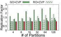
(a) Road-CA

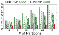
(b) Skitter

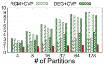
(c) Patent

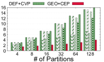
(d) Pokec

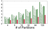
(e) Flickr

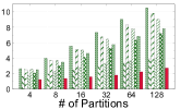
(f) LiveJournal

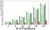
(g) Orkut

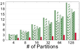
(h) Twitter

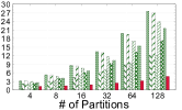
(i) FriendSter

Figure 11: Replication Factor Compared to Graph Ordering Methods.

Partitioning Quality Compared to Graph Ordering Methods. Figure 11 shows the quality evaluation of the graph ordering methods. All the existing methods are vertex ordering. Thus, we partition the ordered vertices via CVP and generate vertex partitions. For quality comparison, we convert vertex partitions into edge partitions in the same way as the previous subsection.

Overall, GEO+CEP is always better than the other ordering methods. Especially, the improvement is significant in Orkut, where the replication factor is totally high, meaning that, it is difficult to get good partitions. RO and LLP become the similar quality to GEO+CEP in Road-CA and Flickr. This is because these two methods capture ‘general’ data locality (i.e., network modularity in RO and community structure in LLP) rather than to solve some problems highly specific to its purpose (i.e., GO is for the L1-cache utilization; and RGB is for graph compression). In Road-CA and Flickr, these general localities become similar to one derived from the graph edge ordering.

The high quality of GEO+CEP essentially comes from the design of the priority (Eq. (8)) derived from the objective of the graph edge ordering problem (Eq. (1) and Eq. (6)). This is due to the fact that some of the existing ordering methods, such as RCM and GO, are based on BFS and an algorithm very close to ours. Our priority differentiates the partitioning quality of GEO+CEP from that of the existing methods.

Preprocessing Time. We compare the elapsed time of each ordering method. Figure 12 shows the result. Although GEO is not the best performance compared to the simple methods, such as RCM and DEG, its performance is similar to the other ordering methods such as GO, RGB, and LLP. The graph edge ordering can preprocess the billion-scale graphs (Twitter and FriendSter) within an acceptable time.

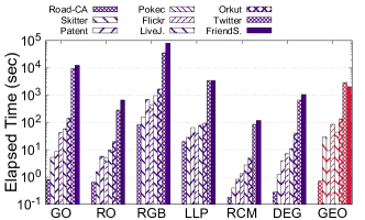
Figure 12: Preprocessing Time for Graph Ordering

6.4 Effect on Distributed Graph Analysis

We briefly evaluate the effect of our dynamic scaling method on three common benchmarking graph applications with different workload characteristics: SSSP, WCC, and PageRank. SSSP is the lightest workload, starting from Vertex $0$ in this evaluation; WCC is the middle one; PageRank is the heaviest one, where all vertices communicate with their neighbors at each iteration (the number of iterations is set to $100$). We integrate our method to PowerLyra Chen:2015:PDG:2741948.2741970 (forked from PowerGraph joseph2012powergraph ) and compare it with four methods in the system: 1D (Random), 2D (Grid), Oblivious, and Hybrid Ginger. For a more comprehensive and detailed analysis of the effect of the partitioning quality on distributed graph applications, please refer to the previous experimental researches Han:2014:ECP:2732977.2732980 ; 6877273 ; Verma:2017:ECP:3055540.3055543 ; abbas2018streaming ; Gill:2018:SPP:3297753.3316427 ; Pacaci:2019:EAS:3299869.3300076 . The result of this evaluation is consistent with these researches.

We use two metrics: the elapsed time (TIME) and the communication volume (COM), as well as three metrics for the quality: the replication factor (RF), the edge balance (EB), and the vertex balance (VB). Specifically, let a balance factor among partitions ($p\in P$) be $B(\{x_{p}\}):=\tfrac{\max x_{p}}{\bar{x}}$, where $\bar{x}:=\tfrac{\sum x_{p}}{|P|}$. Then, EB and VB are defined as $B(\{|E_{p}|\})$ and $B(\{|V(E_{p})|\})$, respectively. Note that EB is the actual value of $1+\epsilon$ as difined in Def. 2.

We evaluate our proposed approach in two different ways: (i) measuring the performance of applications and (ii) measuring the performance of the entire system including dynamic scaling.

6.4.1 Application Performance

Table 6 shows the result on 36 partitions (one physical core per partition) without dynamic scaling by using the three large graphs (Orkut, Twitter, and FriendSter). For the elapsed time (TIME), we measure the time only for applications and exclude setup time such as system preparation, data loading, data partitioning, and so forth. We execute five times and show the median value.

Overall, our method (CEP+GEO) outperforms the others in the elapsed time (TIME) due to the lowest replication factor (RF). Its speed up from the others is the most significant in PageRank due to the largest reduction of communication cost (COM). Even though the vertex balance (VB) of our methods is slightly worse than that of the others, it does not play an important role for the elapsed time (TIME). This is because the computational cost for the graph processing essentially depends on the number of edges rather than that of vertices, as already discussed in Sec. 1. The edge balance is more dominant for the performance, and our method always achieves the perfect score (i.e., EB is 1).

Table 6: Evaluation of Graph Applications on 36 Partitions. TIME unit is sec. COM unit is GB.

		Quality			SSSP		WCC		PageRank
		RF	EB	VB	TIME	COM	TIME	COM	TIME	COM
Orkut	1D	23.91	1.00	1.00	5.29	8.51	22.0	22.5	224	167
	2D (Grid)	9.76	1.01	1.01	3.93	4.30	13.67	9.5	130	69.7
	Oblivious	16.35	1.23	1.01	4.43	6.27	17.0	15.62	168	112
	Hybrid Ginger	11.56	1.37	1.05	3.95	8.25	13.5	12.5	106	56.2
	GEO+CEP	2.98	1.00	1.32	2.89	0.72	8.20	1.99	66.6	15.6
Twitter	1D	14.11	1.00	1.00	47.5	74.1	136	126	2043	1262
	2D (Grid)	7.52	1.04	1.00	31.2	47.5	90.8	72.0	1239	647
	Oblivious	11.04	1.05	1.01	38.4	61.4	108	100	1630	985
	Hybrid Ginger	4.20	1.21	1.06	22.0	75.8	64.9	73.8	717	319
	GEO+CEP	2.20	1.00	2.92	17.6	6.11	47.6	16.2	518	130
FriendS.	1D	14.46	1.00	1.00	81.7	112	389	297	3561	2160
	2D (Grid)	6.74	1.00	1.00	52.5	63.2	261	140	1985	983
	Oblivious	10.91	1.00	1.00	66.9	90.1	306	224	2609	1567
	Hybrid Ginger	7.28	1.14	1.10	51.2	117	241	181	1652	812
	GEO+CEP	2.44	1.00	3.04	39.7	11.4	169	31.1	963	241

6.4.2 End-to-end Performance

We evaluate the entire performance of PageRank (100 iterations) including the setup such as system initialization, graph (re)partitioning, data migration, and graph (re)construction.

Dynamic Scaling Scenario. We use two scenarios: ScaleOut and ScaleIn. In ScaleOut, a process is added each 10 iterations from 26 processes. Thus, the number of partitions is changed as follows: $26\rightarrow 27\rightarrow...\rightarrow 36$. In ScaleIn, a process is removed each 10 iterations from 36 processes. Thus, the number of partitions is changed as follows: $36\rightarrow 35\rightarrow...\rightarrow 26$.

Result. We show the total elapsed time (ALL) and the breakdown of its three constituent components (INIT, APP, and SCALE). INIT is the initialization time including system setup, data loading, initial partitioning and graph construction. APP is the application time for PageRank computation. SCALE includes the repartitioning, data migration (structural data and intermediate values), and graph reconstruction.

As shown in Table 7, our method significantly outperforms the others in ALL due to the large performance improvement not only in APP but also in INIT and SCALE. In INIT, the improvement mainly comes from the efficient partitioning and data loading from the file system. In our method, the partitioning can be computed by directly loading from the file system without any data shuffling among the distributed processes. Whereas, in the other methods, the partition of each edge of a graph needs to be processed one-by-one after data loading. In SCALE, the improvement is mainly due to the efficient repartitioning as discussed in Theorem 3.1.

Table 7: Overall Time (ALL) and its Breakdown (INIT, APP, SCALE) for PageRank with Dynamic Scaling (sec.).

		ScaleOut				ScaleIn
		ALL	INIT	APP	SCALE	ALL	INIT	APP	SCALE
Orkut	1D	301	6.8	220.2	72.9	298	8.0	216.8	72.8
	Oblivious	282	7.8	184.0	89.4	279	7.7	181.9	88.7
	Hybrid Ginger	205	9.0	105.2	90.4	210	9.6	106.3	93.5
	GEO+CEP	96	2.4	71.5	21.7	98	4.8	70.7	22.1
Twitter	1D	2893	75	2042	769	2843	86	1979	771
	Oblivious	2803	95	1673	1030	2767	91	1643	1029
	Hybrid Ginger	1673	114	602	955	1853	290	603	958
	GEO+CEP	837	37	541	257	851	54	532	264
FriendS.	1D	4937	117	3581	1228	4974	123	3569	1274
	Oblivious	4607	126	2990	1482	4576	146	2934	1488
	Hybrid Ginger	3700	198	1583	1915	3684	199	1562	1917
	GE0+CEP	1512	56	1035	418	1487	49	1007	429

6.4.3 Additional Experiment

Migration Cost. We evaluate the migration cost in dynamic scaling (ScaleOut and ScaleIn in the previous section). We use three methods for the comparison: BVC, 1D, and CEP. BVC is designed for the efficient migration as its objective is defined as the minimization of the migration cost. 1D is a representative of the other partitioning methods that do not take the migration cost into account. Each partitioned edge may basically move to any of the other partitions.

Figure 13 shows the number of migrated edges in the two scenarios. BVC and CEP are almost the same number, outperforming 1D. This is due to the fact that the migration methods in BVC and CEP are very similar, where their difference is to align the edges to the ordering id space (CEP) or to the hash ring in consistent hashing (BVC). In both methods, edges are split into the continuous chunks, and thus, the number of migrated edges is almost the same.

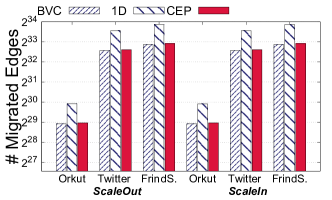
Figure 13: Total # of Migrated Edges in ScaleOut and ScaleIn.

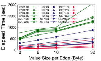
Figure 14: Migration Time for ScaleOut with FriendS..

Figure 14 shows the actual elapsed time to migrate the edges and their values under the different network performances and sizes of each edge value. We emulate the different network bandwidth from 1Gbps to 32Gbps according to the instance specifications in Amazon EC2 instancetype . The size of value per edge is changed from 0 to 32 bytes.

In contrast to the number of migrated edges, CEP and 1D outperform BVC. This is because, in BVC, the edges are communicated in two phases: the initial migration and refinement for balancing edges. The refinement includes a lot of barrier synchronizations to share the edge balanceness among the distributed processes, especially in small $\epsilon$ and $k$. BVC is considered to be more appropriate for larger $\epsilon$ and $k$ as evaluated in dynamicscaling (where $\epsilon$ is around 100 times bigger than our case and $k$ is over 100). On the other hand, in CEP and 1D, the graph data are communicated in the single data shuffling and do not include the multiple global synchronizations.

An interesting insight from the evaluation is that the performance difference/improvement in data migration time is relatively small even though the number of migrated edges is largely different and the data migration itself is time-consuming (in some cases, it is slower than the partitioning time). In contrast, the partitioning time as shown in Figure 9 exhibits a lot of variation in each of the methods examined, and thus its performance improvement may substantially influence the overall workload.

Scalability. Figure 15 shows the scalability of GEO. We use RMAT, a common synthetic model for social networks chakrabarti2004r . According to the real-world social networks in Table 3, we change Edge Factor of RMAT (i.e., average degree) from 16 to 40 and the graph size up to 10 billion-edge scale. Overall, the performance changes linearly as the increase of the graph size. However, GEO as well as its other counterparts (i.e., high-quality graph partitioning and graph ordering methods) have a scalability limitation. That is, if the preprocessing time is very large (e.g., due to the large graph size), whereas the actual analysis time is relatively small (e.g., due to the high parallelization), then the benefit by the preprocessing cannot be amortized. Such a limitation gives us the motivation to devise parallel and distributed algorithms to speed up GEO. This is listed as our future work in Sec. 7.

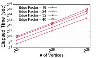
Figure 15: Scalability of GEO with RMAT Graphs.

7 Conclusion and Future Work

In this paper, we presented a novel approach to the dynamic scaling of graph partitions. Our idea is based on the graph edge ordering and the chunk-based edge partitioning. The former is the preprocessing method to provide high-quality partitions. The latter is the very fast $O(1)$ partitioning algorithm. We show that the maximization of the partitioning quality via graph edge ordering is NP-hard. We proposed an efficient greedy algorithm to solve the problem within an acceptable time for large real-world graphs. As a result, once the preprocessing is done, our dynamic scaling method is between three to eight orders of magnitude faster than the other existing methods while achieving high partitioning quality, which is similar to the best existing method.

There are mainly four future directions for our work. First, the graph edge ordering needs to support the dynamic change of graph structures. The requirement to reconfigure the number of partitions and recompute the graph analysis is higher for such dynamic graphs. Second, a parallel and distributed algorithm of the graph edge ordering will be investigated. The current sequential algorithm cannot handle extremely large graphs, such as trillion-edge graphs. Third, the application to more complicated and time-consuming distributed graph processing, such as graph-based machine learning, is a very interesting and attractive problem. Finally, the extension to more complicated graphs, such as, weighted-vertex/edge graphs, hyper graphs, property graphs, temporal graphs, will be investigated.

References

- [1] Grzegorz Malewicz, Matthew H Austern, Aart JC Bik, James C Dehnert, Ilan Horn, Naty Leiser, and Grzegorz Czajkowski. Pregel: a system for large-scale graph processing. In SIGMOD, pages 135–146, 2010.
- [2] Joseph E Gonzalez, Reynold S Xin, Ankur Dave, Daniel Crankshaw, Michael J Franklin, and Ion Stoica. GraphX: Graph processing in a distributed dataflow framework. In OSDI, pages 599–613, 2014.
- [3] Joseph E. Gonzalez, Yucheng Low, Haijie Gu, Danny Bickson, and Carlos Guestrin. PowerGraph: Distributed graph-parallel computation on natural graphs. In OSDI, pages 17–30, 2012.
- [4] Sungpack Hong, Siegfried Depner, Thomas Manhardt, Jan Van Der Lugt, Merijn Verstraaten, and Hassan Chafi. PGX. D: A fast distributed graph processing engine. In SC, pages 58:1–58:12, 2015.
- [5] Rong Chen, Jiaxin Shi, Yanzhe Chen, Binyu Zang, Haibing Guan, and Haibo Chen. PowerLyra: Differentiated graph computation and partitioning on skewed graphs. TOPC, 5(3):13:1–13:39, 2019.
- [6] Michael R Garey, David S Johnson, and Larry Stockmeyer. Some simplified NP-complete problems. In STOC, pages 47–63, 1974.
- [7] Konstantin Andreev and Harald Räcke. Balanced graph partitioning. In SPAA, pages 120–124, 2004.
- [8] Florian Bourse, Marc Lelarge, and Milan Vojnovic. Balanced graph edge partition. In KDD, pages 1456–1465, 2014.
- [9] Chenzi Zhang, Fan Wei, Qin Liu, Zhihao Gavin Tang, and Zhenguo Li. Graph edge partitioning via neighborhood heuristic. In KDD, pages 605–614, 2017.
- [10] George Karypis and Vipin Kumar. A fast and high quality multilevel scheme for partitioning irregular graphs. SISC, 20(1):359–392, 1998.
- [11] Charalampos Tsourakakis, Christos Gkantsidis, Bozidar Radunovic, and Milan Vojnovic. FENNEL: Streaming graph partitioning for massive scale graphs. In WSDM, pages 333–342, 2014.
- [12] Cong Xie, Ling Yan, Wu-Jun Li, and Zhihua Zhang. Distributed power-law graph computing: Theoretical and empirical analysis. In NeurIPS, pages 1673–1681, 2014.
- [13] Fabio Petroni, Leonardo Querzoni, Khuzaima Daudjee, Shahin Kamali, and Giorgio Iacoboni. HDRF: Stream-based partitioning for power-law graphs. In CIKM, pages 243–252, 2015.
- [14] Amazon EC2 Spot Instances. https://aws.amazon.com/ec2/spot/.
- [15] Google Preemptible VMs. https://cloud.google.com/preemptible-vms/.
- [16] Josep M Pujol, Vijay Erramilli, Georgos Siganos, Xiaoyuan Yang, Nikos Laoutaris, Parminder Chhabra, and Pablo Rodriguez. The little engine (s) that could: scaling online social networks. In SIGCOMM, pages 375–386, 2011.
- [17] Luis M Vaquero, Felix Cuadrado, Dionysios Logothetis, and Claudio Martella. Adaptive partitioning for large-scale dynamic graphs. In ICDCS, pages 144–153, 2014.
- [18] S. Heidari and R. Buyya. A cost-efficient auto-scaling algorithm for large-scale graph processing in cloud environments with heterogeneous resources. TSE, 2019. ealry access.
- [19] A. Uta, S. Au, A. Ilyushkin, and A. Iosup. Elasticity in graph analytics? a benchmarking framework for elastic graph processing. In CLUSTER, pages 381–391, 2018.
- [20] Wenfei Fan, Chunming Hu, Muyang Liu, Ping Lu, Qiang Yin, and Jingren Zhou. Dynamic scaling for parallel graph computations. PVLDB, 12(8):877–890, 2019.
- [21] Zechao Shang and Jeffrey Xu Yu. Catch the wind: Graph workload balancing on cloud. In ICDE, pages 553–564, 2013.
- [22] Zuhair Khayyat, Karim Awara, Amani Alonazi, Hani Jamjoom, Dan Williams, and Panos Kalnis. Mizan: a system for dynamic load balancing in large-scale graph processing. In EuroSys, pages 169–182, 2013.
- [23] Ning Xu, Lei Chen, and Bin Cui. LogGP: a log-based dynamic graph partitioning method. PVLDB, 7(14):1917–1928, 2014.
- [24] Jiewen Huang and Daniel J Abadi. Leopard: Lightweight edge-oriented partitioning and replication for dynamic graphs. PVLDB, 9(7):540–551, 2016.
- [25] Angen Zheng, Alexandros Labrinidis, Patrick H Pisciuneri, Panos K Chrysanthis, and Peyman Givi. PARAGON: Parallel architecture-aware graph partition refinement algorithm. In EDBT, pages 365–376, 2016.
- [26] Angen Zheng, Alexandros Labrinidis, and Panos K Chrysanthis. Planar: Parallel lightweight architecture-aware adaptive graph repartitioning. In ICDE, pages 121–132, 2016.
- [27] Trieu C Chieu, Ajay Mohindra, Alexei A Karve, and Alla Segal. Dynamic scaling of web applications in a virtualized cloud computing environment. In ICEBE, pages 281–286, 2009.
- [28] Zhiming Shen, Sethuraman Subbiah, Xiaohui Gu, and John Wilkes. Cloudscale: elastic resource scaling for multi-tenant cloud systems. In SOCC, page 5, 2011.
- [29] Sudipto Das, Shoji Nishimura, Divyakant Agrawal, and Amr El Abbadi. Albatross: lightweight elasticity in shared storage databases for the cloud using live data migration. PVLDB, 4(8):494–505, 2011.
- [30] Sudipto Das, Divyakant Agrawal, and Amr El Abbadi. ElasTraS: An elastic, scalable, and self-managing transactional database for the cloud. TODS, 38(1):5:1–5:45, 2013.
- [31] Rebecca Taft, Essam Mansour, Marco Serafini, Jennie Duggan, Aaron J Elmore, Ashraf Aboulnaga, Andrew Pavlo, and Michael Stonebraker. E-store: Fine-grained elastic partitioning for distributed transaction processing systems. PVLDB, 8(3):245–256, 2014.
- [32] Marco Serafini, Essam Mansour, Ashraf Aboulnaga, Kenneth Salem, Taha Rafiq, and Umar Farooq Minhas. Accordion: Elastic scalability for database systems supporting distributed transactions. PVLDB, 7(12):1035–1046, 2014.
- [33] Atul Adya, Daniel Myers, Jon Howell, Jeremy Elson, Colin Meek, Vishesh Khemani, Stefan Fulger, Pan Gu, Lakshminath Bhuvanagiri, Jason Hunter, et al. Slicer: Auto-sharding for datacenter applications. In USENIX OSDI, pages 739–753, 2016.
- [34] Rebecca Taft, Nosayba El-Sayed, Marco Serafini, Yu Lu, Ashraf Aboulnaga, Michael Stonebraker, Ricardo Mayerhofer, and Francisco Andrade. P-Store: An elastic database system with predictive provisioning. In SIGMOD, pages 205–219, 2018.
- [35] Ryan Marcus, Olga Papaemmanouil, Sofiya Semenova, and Solomon Garber. NashDB: An end-to-end economic method for elastic database fragmentation, replication, and provisioning. In SIGMOD, pages 1253–1267, 2018.
- [36] Atsushi Ishii and Toyotaro Suzumura. Elastic stream computing with clouds. In CLOUD, pages 195–202, 2011.
- [37] Raul Castro Fernandez, Matteo Migliavacca, Evangelia Kalyvianaki, and Peter Pietzuch. Integrating scale out and fault tolerance in stream processing using operator state management. In SIGMOD, pages 725–736, 2013.
- [38] Thomas Heinze, Lars Roediger, Andreas Meister, Yuanzhen Ji, Zbigniew Jerzak, and Christof Fetzer. Online parameter optimization for elastic data stream processing. In SOCC, pages 276–287, 2015.
- [39] Kasper Grud Skat Madsen, Yongluan Zhou, and Jianneng Cao. Integrative dynamic reconfiguration in a parallel stream processing engine. In ICDE, pages 227–230, 2017.
- [40] Avrilia Floratou, Ashvin Agrawal, Bill Graham, Sriram Rao, and Karthik Ramasamy. Dhalion: self-regulating stream processing in heron. PVLDB, 10(12):1825–1836, 2017.
- [41] Michael Borkowski, Christoph Hochreiner, and Stefan Schulte. Minimizing cost by reducing scaling operations in distributed stream processing. PVLDB, 12(7):724–737, 2019.
- [42] LI Wang, Tom Z. J. Fu, Richard T. B. Ma, Marianne Winslett, and Zhenjie Zhang. Elasticutor: Rapid elasticity for realtime stateful stream processing. In SIGMOD, pages 573–588, 2019.
- [43] Ming Mao and Marty Humphrey. Auto-scaling to minimize cost and meet application deadlines in cloud workflows. In SC, pages 1–12, 2011.
- [44] Aurick Qiao, Abutalib Aghayev, Weiren Yu, Haoyang Chen, Qirong Ho, Garth A Gibson, and Eric P Xing. Litz: Elastic framework for high-performance distributed machine learning. In USENIX ATC, pages 631–644, 2018.
- [45] Kangfei Zhao, Yu Rong, Jeffrey Xu Yu, Junzhou Huang, and Hao Zhang. Graph ordering: Towards the optimal by learning, 2020.
- [46] E. Cuthill and J. McKee. Reducing the bandwidth of sparse symmetric matrices. In ACM, pages 157–172, 1969.
- [47] Paolo Boldi, Marco Rosa, Massimo Santini, and Sebastiano Vigna. Layered label propagation: A multiresolution coordinate-free ordering for compressing social networks. In WWW, pages 587–596, 2011.
- [48] Yongsub Lim, U Kang, and Christos Faloutsos. Slashburn: Graph compression and mining beyond caveman communities. TKDE, 26(12):3077–3089, 2014.
- [49] Laxman Dhulipala, Igor Kabiljo, Brian Karrer, Giuseppe Ottaviano, Sergey Pupyrev, and Alon Shalita. Compressing graphs and indexes with recursive graph bisection. KDD, pages 1535–1544, 2016.
- [50] Hao Wei, Jeffrey Xu Yu, Can Lu, and Xuemin Lin. Speedup graph processing by graph ordering. In SIGMOD, pages 1813–1828, 2016.
- [51] Junya Arai, Hiroaki Shiokawa, Takeshi Yamamuro, Makoto Onizuka, and Sotetsu Iwamura. Rabbit order: Just-in-time parallel reordering for fast graph analysis. In IPDPS, pages 22–31, 2016.
- [52] Oshini Goonetilleke, Danai Koutra, Timos Sellis, and Kewen Liao. Edge labeling schemes for graph data. In SSDBM, pages 12:1–12:12, 2017.
- [53] Minyang Han, Khuzaima Daudjee, Khaled Ammar, M. Tamer Özsu, Xingfang Wang, and Tianqi Jin. An experimental comparison of pregel-like graph processing systems. PVLDB, 7(12):1047–1058, 2014.
- [54] Y. Guo, M. Biczak, A. L. Varbanescu, A. Iosup, C. Martella, and T. L. Willke. How well do graph-processing platforms perform? an empirical performance evaluation and analysis. In IPDPS, pages 395–404, 2014.
- [55] Shiv Verma, Luke M. Leslie, Yosub Shin, and Indranil Gupta. An experimental comparison of partitioning strategies in distributed graph processing. PVLDB, 10(5):493–504, 2017.
- [56] Zainab Abbas, Vasiliki Kalavri, Paris Carbone, and Vladimir Vlassov. Streaming graph partitioning: an experimental study. PVLDB, 11(11):1590–1603, 2018.
- [57] Gurbinder Gill, Roshan Dathathri, Loc Hoang, and Keshav Pingali. A study of partitioning policies for graph analytics on large-scale distributed platforms. PVLDB, 12(4):321–334, 2018.
- [58] Anil Pacaci and M. Tamer Özsu. Experimental analysis of streaming algorithms for graph partitioning. In SIGMOD, pages 1375–1392, 2019.
- [59] Masatoshi Hanai, Toyotaro Suzumura, Wen Jun Tan, Elvis Liu, Georgios Theodoropoulos, and Wentong Cai. Distributed edge partitioning for trillion-edge graphs. PVLDB, 12(13):2379–2392, 2019.
- [60] Aaron Clauset, Cosma Rohilla Shalizi, and Mark EJ Newman. Power-law distributions in empirical data. SIAM review, 51(4):661–703, 2009.
- [61] SNAP Datasets. http://snap.stanford.edu/data.
- [62] KONECT. http://konect.cc/.
- [63] Jure Leskovec, Kevin J Lang, Anirban Dasgupta, and Michael W Mahoney. Community structure in large networks: Natural cluster sizes and the absence of large well-defined clusters. Internet Mathematics, 6(1):29–123, 2009.
- [64] Jure Leskovec, Jon Kleinberg, and Christos Faloutsos. Graphs over time: densification laws, shrinking diameters and possible explanations. In KDD, pages 177–187, 2005.
- [65] Lubos Takac and Michal Zabovsky. Data analysis in public social networks. In DTI, volume 1, 2012.
- [66] Alan Mislove, Hema Swetha Koppula, Krishna P. Gummadi, Peter Druschel, and Bobby Bhattacharjee. Growth of the flickr social network. In WOSN, pages 25–30, 2008.
- [67] Lars Backstrom, Dan Huttenlocher, Jon Kleinberg, and Xiangyang Lan. Group formation in large social networks: Membership, growth, and evolution. In KDD, pages 44–54, 2006.
- [68] Jaewon Yang and Jure Leskovec. Defining and evaluating network communities based on ground-truth. KAIS, 42(1):181–213, 2015.
- [69] Haewoon Kwak, Changhyun Lee, Hosung Park, and Sue Moon. What is twitter, a social network or a news media? In WWW, pages 591–600, 2010.
- [70] Jaewon Yang and J Leskovec. Defining and evaluating network communities based on ground-truth. In ICDM, pages 745–754, 2012.
- [71] Xiaowei Zhu, Wenguang Chen, Weimin Zheng, and Xiaosong Ma. Gemini: A computation-centric distributed graph processing system. In OSDI, pages 301–316, 2016.
- [72] Amazon EC2 Instance Types. https://aws.amazon.com/ec2/instance-types/.
- [73] Deepayan Chakrabarti, Yiping Zhan, and Christos Faloutsos. R-MAT: A recursive model for graph mining. In SDM, pages 442–446, 2004.