Space-time block preconditioning for incompressible flow

Abstract

Parallel-in-time methods have become increasingly popular in the simulation of time-dependent numerical PDEs, allowing for the efficient use of additional MPI processes when spatial parallelism saturates. Most methods treat the solution and parallelism in space and time separately. In contrast, all-at-once methods solve the full space-time system directly, largely treating time as simply another spatial dimension. All-at-once methods offer a number of benefits over separate treatment of space and time, most notably significantly increased parallelism and faster time-to-solution (when applicable). However, the development of fast, scalable all-at-once methods has largely been limited to time-dependent (advection-)diffusion problems. This paper introduces the concept of space-time block preconditioning for the all-at-once solution of incompressible flow. By extending well-known concepts of spatial block preconditioning to the space-time setting, we develop a block preconditioner whose application requires the solution of a space-time (advection-)diffusion equation in the velocity block, coupled with a pressure Schur complement approximation consisting of independent spatial solves at each time-step, and a space-time matrix-vector multiplication. The new method is tested on four classical models in incompressible flow. Results indicate perfect scalability in refinement of spatial and temporal mesh spacing, perfect scalability in nonlinear Picard iterations count when applied to a nonlinear Navier-Stokes problem, and minimal overhead in terms of number of preconditioner applications compared with sequential time-stepping.

Key words. Parallel-in-time integration, block preconditioning, incompressible flow, finite element methods

AMS subject classifications. 65F08, 65Y05, 76D07, 65M60

1 Introduction

Parallel-in-Time (PinT) algorithms have received significant attention in recent years because of their potential to expose further concurrency in the numerical solution of partial differential equations (PDEs). At some number of MPI processes, traditional (sequential) time-stepping methods that rely on spatial parallelism reach saturation, that is, further increasing the number of MPI processes no longer reduces the total time to solution. Due to the increasing number of processors available for computation, it is then desirable to also utilise parallelism in the temporal dimension. One of the original PinT algorithms is Parareal [21, 14], introduced by Lions, Maday, and Turinici in 2001, which is essentially a two-level multigrid method in time. Since then, a wide range of approaches for PinT have been developed. For a complete overview of PinT algorithms, we point to the review by Gander [11]. Broadly, we will split time-parallelisation techniques into two categories: (i) PinT methods (excusing the slight abuse of terminology), which treat the temporal dimension and its parallelisation separately from the spatial dimensions, and (ii) all-at-once methods, which treat time and space together, and achieve parallelisation by solving the full monolithic system representing the space-time discretisation of a time-dependent PDE.

A variety of all-at-once methods have been proposed [13, 12, 25, 15, 22]. Some of the most successful ones (particularly for the heat equation) are rooted on multigrid techniques, and directly apply geometric multigrid (GMG) or algebraic multigrid (AMG) to full space-time linear systems [9, 17, 37]. Such an approach naturally allows for adaptive mesh refinement in both space and time [37], and has shown to offer significantly more parallelism and faster time-to-solution [9] compared with PinT methods that treat space and time separately such as Parareal and multigrid reduction in time (MGRIT) [8]. While in general multigrid approaches have been successful for the space-time parallelisation of single-variable (advection-)diffusion equations, to our knowledge no multigrid methods have been developed and proven effective on systems of PDEs in space and time. Indeed, effectively handling at the same time both the complications introduced by inter-variable coupling in systems of PDEs, as well as the purely advective term in one dimension representing a time derivative, is beyond the capabilities of the current state-of-the-art.

Flow problems are a particularly appealing target for time-parallelisation because of their long time dynamics and the high computational cost typically associated with their solution. See [42] for a discussion on the need for time parallelism in numerical fluid dynamics on emerging architectures. In this paper, we focus on incompressible flow. Parareal has been applied to incompressible flows in a number of works, e.g., [27, 41, 40, 3, 10], which have generally shown successful results. Save for few exceptions, in most of the articles listed above the treatment of space and time is still kept separate, and one does not get the same benefits that can arise from a true all-at-once approach. A number of papers have also considered the all-at-once discretisation of incompressible flow using space-time finite elements (for example, see [32, 31]), but to our knowledge, none of these papers have developed efficient, parallel methods for the all-at-once solution of such space-time discretisations.

In this paper, we take a new approach and develop a space-time block preconditioner for the all-at-once solution of incompressible flow. Applying our preconditioner requires solving a space-time advection-diffusion equation involving only the velocity variable, and inverting an approximate space-time pressure Schur complement. The latter relies on the solution of a pressure Laplacian and mass matrix at each time-step; these are independent for each time instant, which makes this procedure naturally parallel in time. For the former, there already exist efficient methods for the time-parallel solution of single-variable advection-diffusion equations, and their development remains more tractable than for the fully-coupled space-time system. The block separation introduced by our preconditioner allows for great freedom in the choice of the solver for the velocity block, and it makes it straightforward to apply, e.g., space-time multigrid as in [9, 17, 37]. The proposed method takes motivation from well-developed spatial block preconditioning techniques used in sequential time-stepping or steady-state problems [5]. The development of many such methods is based on a commuting argument involving some spatial operators, which then allows one to find an effective approximation of the Schur complement. Noting that formally (that is, without boundary conditions) spatial and temporal derivatives commute, we claim that similar principles can be generalised to the space-time setting, where an additional time derivative is present. Indeed, in section 3, our preconditioner is derived using multiple different frameworks that can be seen as natural extensions from the spatial block preconditioning setting.

Similar in spirit to this paper is the approach described in [39], where the authors propose a preconditioner for a time-dependent optimal control problem, exploiting the block structure of the system at the space-time level. However, to our knowledge, similar concepts have not been applied before for the purpose of time-parallelisation. Moreover, while our focus in this manuscript is incompressible flow, we believe the underlying principle of space-time block preconditioning can be extended to other systems of PDEs for which effective spatial block preconditioners have been developed for the single time-step case (or for its stationary counterpart).

The content of this article is as follows. Section 2 introduces our target problem, together with notation that will be used throughout the paper. A derivation of the space-time block preconditioner representing our main contribution is given in section 3, together with multiple theoretical justifications. In section 4 we investigate the effectiveness of the proposed preconditioner, testing its performance on four classical models in incompressible flow. Results indicate perfect scalability in refinement of spatial and temporal mesh spacing, perfect scalability in nonlinear Picard iteration count when applied to a nonlinear Navier-Stokes problem, and minimal overhead in terms of number of preconditioner applications compared with sequential time-stepping. Section 5 summarises our findings and discusses directions for future work.

2 Problem definition and discretisation

This section introduces notation that is used throughout the manuscript. Here we describe a time-dependent version of the Oseen equations, as well as the discrete operators arising from its finite element discretisation.

Our target system is

$$\left\{\begin{array}[]{lr}\begin{array}[]{rcl}\displaystyle\frac{\partial{\boldsymbol{u}}}{\partial t}({\boldsymbol{x}},t)+({\boldsymbol{w}}({\boldsymbol{x}},t)\cdot\nabla){\boldsymbol{u}}({\boldsymbol{x}},t)\\ -\mu\nabla^{2}{\boldsymbol{u}}({\boldsymbol{x}},t)+\nabla p({\boldsymbol{x}},t)&=&{\boldsymbol{f}}({\boldsymbol{x}},t)\rule[-3.87495pt]{0.0pt}{0.0pt}\\ \nabla\cdot{\boldsymbol{u}}({\boldsymbol{x}},t)&=&0\rule{0.0pt}{11.19443pt}\end{array}&\quad\text{in}\;\Omega\times(T_{0},T],\\ \end{array}\right.$$ (1)

defined on a spatial domain $\Omega\subset\mathbb{R}^{d}$. Its unknowns are the $d$-dimensional vector field ${\boldsymbol{u}}({\boldsymbol{x}},t)$, and the scalar field $p({\boldsymbol{x}},t)$, representing velocity and pressure, respectively; $\mu$ is the viscosity coefficient, which we consider constant on $\Omega$. The vector function ${\boldsymbol{f}}({\boldsymbol{x}},t)$ is a given forcing term, while ${\boldsymbol{w}}({\boldsymbol{x}},t)$ represents a given $d$-dimensional advection field. The special case where ${\boldsymbol{w}}({\boldsymbol{x}},t)\equiv 0$ gives rise to a time-dependent version of Stokes equations:

$$\left\{\begin{array}[]{lr}\begin{array}[]{rcl}\displaystyle\frac{\partial{\boldsymbol{u}}}{\partial t}({\boldsymbol{x}},t)-\mu\nabla^{2}{\boldsymbol{u}}({\boldsymbol{x}},t)+\nabla p({\boldsymbol{x}},t)&=&{\boldsymbol{f}}({\boldsymbol{x}},t)\rule[-3.87495pt]{0.0pt}{0.0pt}\\ \nabla\cdot{\boldsymbol{u}}({\boldsymbol{x}},t)&=&0\rule{0.0pt}{11.19443pt}\end{array}&\quad\text{in}\;\Omega\times(T_{0},T].\\ \end{array}\right.$$ (2)

While most of the analysis conducted in this paper considers the more general problem 1, we will at times refer to 2 for some simplifications. Conversely, by introducing the nonlinearity ${\boldsymbol{w}}({\boldsymbol{x}},t)\equiv{\boldsymbol{u}}({\boldsymbol{x}},t)$ we produce the Navier-Stokes equations for incompressible flow

$$\left\{\begin{array}[]{lr}\begin{array}[]{rcl}\displaystyle\frac{\partial{\boldsymbol{u}}}{\partial t}({\boldsymbol{x}},t)+({\boldsymbol{u}}({\boldsymbol{x}},t)\cdot\nabla){\boldsymbol{u}}({\boldsymbol{x}},t)\\ -\mu\nabla^{2}{\boldsymbol{u}}({\boldsymbol{x}},t)+\nabla p({\boldsymbol{x}},t)&=&{\boldsymbol{f}}({\boldsymbol{x}},t)\rule[-3.87495pt]{0.0pt}{0.0pt}\\ \nabla\cdot{\boldsymbol{u}}({\boldsymbol{x}},t)&=&0\rule{0.0pt}{11.19443pt}\end{array}&\quad\text{in}\;\Omega\times(T_{0},T].\\ \end{array}\right.$$ (3)

The Oseen system can then be interpreted as a linearisation of Navier-Stokes, implying that the analysis conducted here can be extended to more general frameworks: this is addressed more in detail in section 4.3.

In order to provide closure to the definition of the initial-boundary value problem, we also equip 1 with an initial condition

$${\boldsymbol{u}}({\boldsymbol{x}},T_{0})=\bar{{\boldsymbol{u}}}^{0}({\boldsymbol{x}})\quad\text{on }\Omega,$$ (4)

and appropriate boundary conditions (BC)

$$\begin{array}[]{rcll}{\boldsymbol{u}}({\boldsymbol{x}},t)&=&{\boldsymbol{u}}_{D}({\boldsymbol{s}},t)&\text{on }\Gamma_{D}\times(T_{0},T],\quad\text{and}\rule[-3.87495pt]{0.0pt}{0.0pt}\\ \mu\nabla{\boldsymbol{u}}({\boldsymbol{s}},t)\,{\boldsymbol{n}}({\boldsymbol{s}})-p({\boldsymbol{s}},t)\,{\boldsymbol{n}}({\boldsymbol{s}})&=&{\boldsymbol{g}}({\boldsymbol{s}},t)&\text{on }\Gamma_{N}\times(T_{0},T],\rule{0.0pt}{11.19443pt}\end{array}$$ (5)

where we split the boundary $\partial\Omega$ into its Dirichlet and Neumann parts, respectively, with $\partial\Omega=\Gamma_{D}\cup\Gamma_{N}$ and $\Gamma_{D}\cap\Gamma_{N}=\varnothing$. In 5, ${\boldsymbol{n}}({\boldsymbol{s}})\in\mathbb{R}^{d}$ represents the outward-pointing normal to the boundary, while ${\boldsymbol{u}}_{D}({\boldsymbol{s}},t)$, ${\boldsymbol{g}}({\boldsymbol{s}},t)$, and $\bar{{\boldsymbol{u}}}^{0}({\boldsymbol{x}})$ are some known functions.

At any given instant $t\in\left[T_{0},T\right]$, the velocity unknown lives in the functional space [30, Chap. 2.4.2]

$${\boldsymbol{u}}(\cdot,t)\in V(\Omega)\equiv\left(H^{1}_{\Gamma_{D}}(\Omega)\right)^{d},$$ (6)

including the Dirichlet condition in the form of ${\boldsymbol{u}}_{D}$, while for the pressure we have

$$p(\cdot,t)\in Q(\Omega)\equiv L^{2}(\Omega),\quad\text{or}\quad Q(\Omega)\equiv L^{2}_{0}(\Omega)=\left\{q({\boldsymbol{x}})\in L^{2}(\Omega):\int_{\Omega}q({\boldsymbol{x}})\,d{\boldsymbol{x}}=0\right\},$$ (7)

where the zero-mean valued counterpart, $L^{2}_{0}(\Omega)$, is chosen if Dirichlet boundary conditions are imposed everywhere on the boundary of the domain, $\Gamma_{D}\equiv\partial\Omega$. In either case, having introduced 6 and 7, we can provide the weak formulation [30, Chap. 17.2] of 1: we seek ${\boldsymbol{u}}({\boldsymbol{x}},t)$ and $p({\boldsymbol{x}},t)$ such that

$$\left\{\begin{array}[]{rcll}\displaystyle\frac{\partial}{\partial t}\left\langle{\boldsymbol{u}},{\boldsymbol{v}}\right\rangle+\mu\left\langle\nabla{\boldsymbol{u}},\nabla{\boldsymbol{v}}\right\rangle&&&\\ \displaystyle+\left\langle({\boldsymbol{w}}\cdot\nabla){\boldsymbol{u}},{\boldsymbol{v}}\right\rangle-\left\langle p,\nabla\cdot{\boldsymbol{v}}\right\rangle&=&\left\langle{\boldsymbol{f}},{\boldsymbol{v}}\right\rangle+\displaystyle\int_{\Gamma_{N}}{\boldsymbol{g}}\cdot{\boldsymbol{v}}&\quad\forall{\boldsymbol{v}}({\boldsymbol{x}})\in V(\Omega)\rule[-3.87495pt]{0.0pt}{0.0pt}\\ \displaystyle-\left\langle q,\nabla\cdot{\boldsymbol{u}}\right\rangle&=&0&\quad\forall q({\boldsymbol{x}})\in Q(\Omega)\rule{0.0pt}{11.19443pt}\\ \end{array},\right.$$ (8)

for each instant $t\in(T_{0},T]$, where $\left\langle{\boldsymbol{a}}({\boldsymbol{x}}),{\boldsymbol{b}}({\boldsymbol{x}})\right\rangle=\int_{\Omega}{\boldsymbol{a}}({\boldsymbol{x}})\cdot{\boldsymbol{b}}({\boldsymbol{x}})\,d{\boldsymbol{x}}$ denotes the spatial scalar product (notice we dropped the variables’ dependence on ${\boldsymbol{x}}$ and $t$ in order to contract notation).

Space-time discretisation

The temporal derivative in 8 is discretised using implicit Euler. To this end, we introduce a uniformly-spaced grid, $\{t_{k}\}$, over the temporal domain, where

$$t_{k}=T_{0}+k\Delta t,\qquad\text{with}\qquad\Delta t=(T-T_{0})/N_{t}\qquad\text{and}\qquad k=0,\dots,N_{t},$$ (9)

at whose nodes we seek to recover our numerical solution. Following a finite element approach [30, Chap. 4] [5, Chap. 10], we discretise 8 in space by introducing a triangularisation of $\Omega$ of characteristic length $\Delta x$, on which we build finite-dimensional approximations to both $V(\Omega)$ and $Q(\Omega)$, named $V_{h}(\Omega)$ and $Q_{h}(\Omega)$. These are identified by their basis functions

$$V_{h}(\Omega) \coloneqq\operatorname*{span}\{{\boldsymbol{\phi}}_{0}({\boldsymbol{x}}),\dots,{\boldsymbol{\phi}}_{N_{{\boldsymbol{u}}}-1}({\boldsymbol{x}})\},\quad\text{and}\quad$$ (10a)

$$Q_{h}(\Omega) \coloneqq\operatorname*{span}\{\psi_{0}({\boldsymbol{x}}),\dots,\psi_{N_{p}-1}({\boldsymbol{x}})\},$$ (10b)

with $N_{{\boldsymbol{u}}}$ and $N_{p}$ being the number of degrees of freedom associated with the velocity and pressure variables, respectively, so that vectors ${\boldsymbol{v}}\in\mathbb{R}^{N_{{\boldsymbol{u}}}}$ and ${\boldsymbol{q}}\in\mathbb{R}^{N_{p}}$ correspond to functions in $V_{h}(\Omega)$ and $Q_{h}(\Omega)$ via

$${\boldsymbol{v}}({\boldsymbol{x}})=\sum_{j=0}^{N_{{\boldsymbol{v}}}-1}\left[{\boldsymbol{v}}\right]_{j}{\boldsymbol{\phi}}_{j}({\boldsymbol{x}})\qquad\text{and}\qquad q({\boldsymbol{x}})=\sum_{j=0}^{N_{p}-1}\left[{\boldsymbol{q}}\right]_{j}\psi_{j}({\boldsymbol{x}}),$$ (11)

respectively. In the remainder of the manuscript, we will refer somewhat interchangeably to functions in our discrete spaces and their vector representations according to the bases (10). With this, we can assemble the Galerkin matrices, namely the discrete counterparts of the bilinear forms appearing in (8). In particular, we define the mass and stiffness matrices for the velocity variable, respectively,

$$\left[{\mathcal{M}}_{{\boldsymbol{u}}}\right]_{m,n=0}^{N_{{\boldsymbol{u}}}-1} \coloneqq\int_{\Omega}{\boldsymbol{\phi}}_{m}({\boldsymbol{x}})\cdot{\boldsymbol{\phi}}_{n}({\boldsymbol{x}})\,d{\boldsymbol{x}}\quad\text{and}\quad$$ (12a)

$$\left[{\mathcal{A}}_{{\boldsymbol{u}}}\right]_{m,n=0}^{N_{{\boldsymbol{u}}}-1} \coloneqq\int_{\Omega}\nabla{\boldsymbol{\phi}}_{m}({\boldsymbol{x}})\colon\nabla{\boldsymbol{\phi}}_{n}({\boldsymbol{x}})\,d{\boldsymbol{x}},$$ (12b)

the discrete (negative) divergence matrix, responsible for the coupling between velocity and pressure,

$$\left[{\mathcal{B}}\right]_{m,n=0}^{N_{p}-1,N_{{\boldsymbol{u}}}-1}\coloneqq-\int_{\Omega}{\psi}_{m}({\boldsymbol{x}})\nabla\cdot{\boldsymbol{\phi}}_{n}({\boldsymbol{x}})\,d{\boldsymbol{x}},$$ (13)

and discretisations of the advection operator for each temporal instant $t_{k}$ in 9:

$$\left[{\mathcal{W}}_{{\boldsymbol{u}},k}\right]_{m,n=0}^{N_{{\boldsymbol{u}}}-1}\coloneqq\int_{\Omega}\left(\left({\boldsymbol{w}}({\boldsymbol{x}},t_{k})\cdot\nabla\right){\boldsymbol{\phi}}_{n}({\boldsymbol{x}})\right)\cdot{\boldsymbol{\phi}}_{m}({\boldsymbol{x}})\,d{\boldsymbol{x}}.$$ (14)

Combining spatial and temporal discretisations gives rise to the following discrete linear system approximating 8:

$$\left\{\begin{array}[]{rl}\displaystyle\frac{1}{\Delta t}{\mathcal{M}}_{{\boldsymbol{u}}}\left({\boldsymbol{u}}^{k}-{\boldsymbol{u}}^{k-1}\right)+\mu{\mathcal{A}}_{{\boldsymbol{u}}}{\boldsymbol{u}}^{k}+{\mathcal{W}}_{{\boldsymbol{u}},k}{\boldsymbol{u}}^{k}+{\mathcal{B}}^{T}{\boldsymbol{p}}^{k}&={\boldsymbol{f}}^{k}\\ {\mathcal{B}}{\boldsymbol{u}}^{k}&={\boldsymbol{0}}\end{array}\right.,\quad k=1,\dots N_{t},$$ (15)

where ${\boldsymbol{0}}$ is an all-zero vector of size $N_{p}$. Here, $\left[{\boldsymbol{u}}^{k}\right]_{j}$ and $\left[{\boldsymbol{p}}^{k}\right]_{j}$ represent the coefficients corresponding to the $j$-th basis function for the velocity and pressure variables in 10a and 10b, respectively, evaluated at the $k$-th temporal instant; analogously, $[{\boldsymbol{f}}^{k}]_{j}$ identifies the $L^{2}$-projection of the right-hand side of 8 on the $j$-th basis function for $V_{h}(\Omega)$, at the instant $t_{k}$:

$$[{\boldsymbol{f}}^{k}]_{j}\coloneqq\int_{\Omega}{\boldsymbol{f}}({\boldsymbol{x}},t_{k})\cdot{\boldsymbol{\phi}}_{j}({\boldsymbol{x}})\,d{\boldsymbol{x}}+\int_{\Gamma_{N}}{\boldsymbol{g}}({\boldsymbol{s}},t_{k})\cdot{\boldsymbol{\phi}}_{j}({\boldsymbol{s}})\,d{\boldsymbol{s}}.$$ (16)

We now have all the ingredients necessary to assemble the monolithic space-time system corresponding to (15). To simplify notation, we introduce the operators

$${\mathcal{F}}_{{\boldsymbol{u}},k}\coloneqq\frac{{\mathcal{M}}_{{\boldsymbol{u}}}}{\Delta t}+\mathcal{W}_{{\boldsymbol{u}},k}+\mu{\mathcal{A}}_{{\boldsymbol{u}}},\quad\quad k=1,\dots N_{t}.$$ (17)

We can then arrange all the equations of 15 in a single block matrix, as

(18)

where, with a slight abuse of notation, we re-define ${\boldsymbol{f}}^{1}$ from 16 in order to include the initial condition 4,

$$\left[{\boldsymbol{f}}^{1}\right]_{j}\coloneqq\int_{\Omega}\left({\boldsymbol{f}}({\boldsymbol{x}},t_{1})+\frac{1}{\Delta t}\bar{{\boldsymbol{u}}}^{0}({\boldsymbol{x}})\right)\cdot{\boldsymbol{\phi}}_{j}({\boldsymbol{x}})\,d{\boldsymbol{x}}+\int_{\Gamma_{N}}{\boldsymbol{g}}({\boldsymbol{s}},t_{k})\cdot{\boldsymbol{\phi}}_{j}({\boldsymbol{s}})\,d{\boldsymbol{s}}.$$ (19)

Notice that the system in 18 is of the block lower-triangular structure typical of space-time discretisations [14, 8]; moreover, since we use a one-step method to approximate the time derivative, the system is made of two block diagonals, with the $2\times 2$ blocks composing them highlighted in 18. Usually, the solution to 15 is recovered via a time-stepping routine, which corresponds to solving 18 directly via (block) forward substitution. There are several methods to accelerate this procedure, mostly focusing on accelerating the inversion of the main diagonal blocks

$${\mathcal{A}}_{k}\coloneqq\left[\begin{array}[]{cc}{\mathcal{F}}_{{\boldsymbol{u}},k}&{\mathcal{B}}^{T}\\ {\mathcal{B}}\end{array}\right],\qquad k=1,\dots,N_{t},$$ (20)

by designing an optimal preconditioner (see for example [30, Chap. 17.8], or [5, Chap. 4] for an overview). The pressure convection-diffusion (PCD) preconditioner is one of the most successful among these [36], preconditioning the block structure of 20 by finding an accurate and computable approximation to the pressure Schur complement. Our work stems from the same principles as PCD, but considers the whole space-time system 18, rather than just the spatial diagonal blocks 20. Motivation and derivation of our preconditioner are described in the following section.

3 Space-time block-preconditioning

Rather than inverting 18 using sequential time-stepping (i.e., forward substitution), here we tackle the solution of the full space-time system 18 all at once by using preconditioned GMRES [35], with an appropriate space-time block preconditioner. In particular, we focus on developing a preconditioner that treats space and time together and in parallel, which may yield faster time-to-solution than block forward substitution when sufficient processors are available. In the remainder of this section, we show how we can effectively build on concepts developed in the study of the single time-step matrix 20 to design preconditioners that are effective in the full space-time setting.

To develop our preconditioner, we start by reordering the space-time operator in 18 to take the form

(21)

This rearrangement favours a separation of variables based on the physical unknown they refer to, rather than on the individual time-steps. We further denote the blocks composing 21 by

$$F_{{\boldsymbol{u}}}\coloneqq\left[\begin{array}[]{ccc}{\mathcal{F}}_{{\boldsymbol{u}},1}&&\\ -\frac{{\mathcal{M}}_{{\boldsymbol{u}}}}{\Delta t}&\ddots&\\ &\ddots&{\mathcal{F}}_{{\boldsymbol{u}},N_{t}}\end{array}\right],\qquad\text{and}\qquad B\coloneqq\operatorname*{diag}_{N_{t}}({\mathcal{B}}),$$ (22)

where $\operatorname*{diag}_{N}(*)$ denotes a block diagonal matrix with $N$ blocks containing $(*)$. As in the single time-step case [5, Chap. 9.2], we exploit the block structure of 21, and look for a right preconditioner for GMRES in the following block upper triangular form:

$$P_{T}\coloneqq\left[\begin{array}[]{cc}F_{\boldsymbol{u}}&B^{T}\\ &-X\end{array}\right]\quad\Longleftrightarrow\quad P_{T}^{-1}\coloneqq\left[\begin{array}[]{cc}F_{\boldsymbol{u}}^{-1}&F_{\boldsymbol{u}}^{-1}B^{T}X^{-1}\\ &-X^{-1}\end{array}\right],$$ (23)

where $X$ approximates the space-time pressure Schur complement

$$X\approx S_{p}\coloneqq BF_{\boldsymbol{u}}^{-1}B^{T}.$$ (24)

Convergence of GMRES applied to the full space-time system and preconditioned by $P_{T}^{-1}$ is then exactly defined by convergence of GMRES applied to the Schur-complement problem, preconditioned by $X^{-1}$ [38].

The key advantage of the reordering in 21 and the block preconditioning discussed above is that we have effectively decoupled the imposition of the Lagrangian constraint from the solution of the PDE. Applying the preconditioner then requires inverting $F_{\boldsymbol{u}}$ (that is, time-integrating the velocity field), and applying an approximate Schur complement inverse 24. The former represents the discretisation of a single-variable parabolic PDE, which is much simpler to solve in parallel in space-time than the fully-coupled system 21; indeed parallel-in-time and -space-time algorithms have shown to behave well on such problems [9, 37]. Moreover, we claim that the pressure Schur complement 24 can naturally be approximated in a time-parallel fashion. To derive such an approximation, we follow two approaches which have been inspirational in designing efficient preconditioners for the single time-step case.

Remark 1.

One could also consider a block diagonal preconditioner, but due to the nonsymmetry of 22 and 24, MINRES [28] cannot be applied, thus negating one of the primary benefits of using a preconditioner in this form. With GMRES, block diagonal preconditioners are typically expected to require twice as many iterations [38] as block triangular ones, and in this case offer only a marginal reduction in computational cost. Block lower triangular preconditioning is another option, but numerical tests (not included here) have favoured using an upper triangular preconditioner. The latter is also more suited for right-preconditioning [38], which is required by flexible GMRES [34] (and flexible Krylov methods are necessary if we use an inner Krylov method to approximately invert $F_{\boldsymbol{u}}$). For these reasons, $P_{T}$ 23 remains our preconditioner of choice.

3.1 Small commutator approach

In [36], an effective preconditioning strategy for 20 is recovered by starting from an assumption on the commuting of certain operators. Although our Schur complement 24 differs from the case considered there, as it involves a time-derivative, we can still follow a similar line of reasoning. Let us begin by characterising our space-time Schur complement in more detail. Firstly, we can explicitly write $F_{\boldsymbol{u}}^{-1}$ in the following form:

$$F_{\boldsymbol{u}}^{-1}=\left[\begin{array}[]{ccc}{\mathcal{F}}_{{\boldsymbol{u}},1}^{-1}&&\\ {\mathcal{F}}_{{\boldsymbol{u}},2}^{-1}\left(\frac{{\mathcal{M}}_{{\boldsymbol{u}}}}{\Delta t}{\mathcal{F}}_{{\boldsymbol{u}},1}^{-1}\right)&{\mathcal{F}}_{{\boldsymbol{u}},2}^{-1}&\\ {\mathcal{F}}_{{\boldsymbol{u}},3}^{-1}\left(\frac{{\mathcal{M}}_{{\boldsymbol{u}}}}{\Delta t}{\mathcal{F}}_{{\boldsymbol{u}},2}^{-1}\frac{{\mathcal{M}}_{{\boldsymbol{u}}}}{\Delta t}{\mathcal{F}}_{{\boldsymbol{u}},1}^{-1}\right)&{\mathcal{F}}_{{\boldsymbol{u}},3}^{-1}\left(\frac{{\mathcal{M}}_{{\boldsymbol{u}}}}{\Delta t}{\mathcal{F}}_{{\boldsymbol{u}},2}^{-1}\right)&\ddots\\ \vdots&\ddots&\ddots\\ \end{array}\right].$$ (25)

Multiplying on the left and right by the block diagonal matrices $B$ and $B^{T}$, respectively, results in inner operators (i.e., blocks) of the form

$${\mathcal{B}}{\mathcal{F}}_{{\boldsymbol{u}},k}^{-1}\left(\prod_{i=1}^{j}\left(\frac{{\mathcal{M}}_{{\boldsymbol{u}}}}{\Delta t}{\mathcal{F}}_{{\boldsymbol{u}},k-i}^{-1}\right)\right){\mathcal{B}}^{T},\quad\text{with}\quad\left\{\begin{array}[]{l}k=1,\dots,N_{t}\\ j=0,\dots,k-1\end{array}\right.,$$ (26)

where the product is assumed to expand towards the right, i.e., $\prod_{i=0}^{k}a_{i}=a_{0}\prod_{i=1}^{k}a_{i}$, and returns identity if the subscript is larger than the superscript. We seek to adequately approximate the operators appearing in 26: to do so, we follow [36] as well as [5, Chap. 9.2], and make the assumption that the reaction-advection-diffusion operator and the gradient operator approximately commute, that is:

$$\nabla\left(\frac{{\mathcal{I}}}{\Delta t}+\left({\boldsymbol{w}}({\boldsymbol{x}},t)\cdot\nabla\right)-\mu\nabla^{2}\right)-\left(\frac{{\mathcal{I}}}{\Delta t}+\left({\boldsymbol{w}}({\boldsymbol{x}},t)\cdot\nabla\right)-\mu\nabla^{2}\right)\nabla\approx 0.$$ (27)

Notice that the “reaction” term stems from the presence of the temporal derivative, and is mimicked by the scaled identity operator ${\mathcal{I}}/\Delta t$, which automatically commutes with the gradient operator. To provide a discrete analogous of 27, let us define, for each ${\mathcal{F}}_{{\boldsymbol{u}},k}$ in 17, an equivalent reaction-advection-diffusion operator acting on the pressure field:

$$\begin{split}{\mathcal{F}}_{p,k}\coloneqq&\frac{{\mathcal{M}}_{p}}{\Delta t}+\mathcal{W}_{p,k}+\mu{\mathcal{A}}_{p},\qquad k=1,\dots,N_{t},\end{split}$$ (28)

where ${\mathcal{M}}_{p}$, ${\mathcal{A}}_{p}$, and ${\mathcal{W}}_{p,k}$ play the same role as the mass, stiffness, and advection matrices (12a, 12b, and 14), but for the pressure variable, namely

$$\left[{\mathcal{M}}_{p}\right]_{m,n=0}^{N_{p}-1} \coloneqq\int_{\Omega}\psi_{m}({\boldsymbol{x}})\psi_{n}({\boldsymbol{x}})\,d{\boldsymbol{x}},$$ (29a)

$$\left[{\mathcal{A}}_{p}\right]_{m,n=0}^{N_{p}-1} \coloneqq\int_{\Omega}\nabla\psi_{m}({\boldsymbol{x}})\cdot\nabla\psi_{n}({\boldsymbol{x}})\,d{\boldsymbol{x}},\quad\text{and}$$ (29b)

$$\left[{\mathcal{W}}_{p,k}\right]_{m,n=0}^{N_{p}-1} \coloneqq\int_{\Omega}\left({\boldsymbol{w}}({\boldsymbol{x}},t_{k})\cdot\nabla\right)\psi_{n}({\boldsymbol{x}})\psi_{m}({\boldsymbol{x}})\,d{\boldsymbol{x}},\quad\text{for}\quad k=1,\dots,N_{t}.$$ (29c)

More details on how to assemble these operators are provided in section 3.1.2. Translating the commutation assumption to the discrete form introduced in section 2, we have

$$\left({\mathcal{M}}_{{\boldsymbol{u}}}^{-1}{\mathcal{B}}^{T}\right)\left({\mathcal{M}}_{p}^{-1}{\mathcal{F}}_{p,j}\right)-\left({\mathcal{M}}_{{\boldsymbol{u}}}^{-1}{\mathcal{F}}_{{\boldsymbol{u}},j}\right)\left({\mathcal{M}}_{{\boldsymbol{u}}}^{-1}{\mathcal{B}}^{T}\right)\approx 0$$ (30)

for each $j=1,\dots,N_{t}$. Here, re-scaling by the corresponding mass matrices is necessary, since the Galerkin operators have the effect of mapping functions to functionals, integrating over the whole spatial domain.

To get closer to our desired operators 26, we left-multiply 30 by ${\mathcal{F}}_{{\boldsymbol{u}},j}^{-1}{\mathcal{M}}_{{\boldsymbol{u}}}$ and right-multiply by ${\mathcal{F}}_{p,j}^{-1}{\mathcal{M}}_{p}$, thus obtaining

$${\mathcal{F}}_{{\boldsymbol{u}},j}^{-1}{\mathcal{B}}^{T}\approx{\mathcal{M}}_{{\boldsymbol{u}}}^{-1}{\mathcal{B}}^{T}{\mathcal{F}}_{p,j}^{-1}{\mathcal{M}}_{p}.$$ (31)

Continuing to left-multiply by ${\mathcal{F}}_{{\boldsymbol{u}},j+i}^{-1}\frac{{\mathcal{M}}_{{\boldsymbol{u}}}}{\Delta t}$, increasing $i$ until we reach $j+i=k$, using 31 for each $j+i$, and finally left-multiplying by ${\mathcal{B}}$, gives us

$$\begin{split}&{\mathcal{F}}_{{\boldsymbol{u}},j+1}^{-1}\left(\frac{{\mathcal{M}}_{{\boldsymbol{u}}}}{\Delta t}{\mathcal{F}}_{{\boldsymbol{u}},j}^{-1}\right){\mathcal{B}}^{T}\approx\underbrace{\frac{{\mathcal{F}}_{{\boldsymbol{u}},j+1}^{-1}}{\Delta t}{\mathcal{B}}^{T}}_{\approx{\mathcal{M}}_{{\boldsymbol{u}}}^{-1}{\mathcal{B}}^{T}{\mathcal{F}}_{p,j+1}^{-1}\frac{{\mathcal{M}}_{p}}{\Delta t}}{\mathcal{F}}_{p,j}^{-1}{\mathcal{M}}_{p}\\ \Longrightarrow\quad&{\mathcal{B}}{\mathcal{F}}_{{\boldsymbol{u}},k}^{-1}\left(\prod_{i=j}^{k-1}\left(\frac{{\mathcal{M}}_{{\boldsymbol{u}}}}{\Delta t}{\mathcal{F}}_{{\boldsymbol{u}},i}^{-1}\right)\right){\mathcal{B}}^{T}\approx{\mathcal{B}}{\mathcal{M}}_{{\boldsymbol{u}}}^{-1}{\mathcal{B}}^{T}{\mathcal{F}}_{p,k}^{-1}\left(\prod_{i=j}^{k-1}\left(\frac{{\mathcal{M}}_{p}}{\Delta t}{\mathcal{F}}_{p,i}^{-1}\right)\right){\mathcal{M}}_{p},\end{split}$$ (32)

for any desired index $k=1,\dots,N_{t}$. This produces an approximation for each of the operators in 26, and consequently identifies the following candidate for a reasonable approximation of the whole space-time pressure Schur complement 24:

$$X\coloneqq\operatorname*{diag}_{N_{t}}({\mathcal{B}}{\mathcal{M}}_{{\boldsymbol{u}}}^{-1}{\mathcal{B}}^{T})\left[\begin{array}[]{ccc}{\mathcal{F}}_{p,1}^{-1}&&\\ {\mathcal{F}}_{p,2}^{-1}\left(\frac{{\mathcal{M}}_{p}}{\Delta t}{\mathcal{F}}_{p,1}^{-1}\right)&{\mathcal{F}}_{p,2}^{-1}&\\ {\mathcal{F}}_{p,3}^{-1}\left(\frac{{\mathcal{M}}_{p}}{\Delta t}{\mathcal{F}}_{p,2}^{-1}\frac{{\mathcal{M}}_{p}}{\Delta t}{\mathcal{F}}_{p,1}^{-1}\right)&{\mathcal{F}}_{p,3}^{-1}\left(\frac{{\mathcal{M}}_{p}}{\Delta t}{\mathcal{F}}_{p,2}^{-1}\right)&\ddots\\ \vdots&\ddots&\ddots\\ \end{array}\right]\operatorname*{diag}_{N_{t}}({\mathcal{M}}_{p}).$$ (33)

The expression above can be simplified by noticing that the central matrix shares the same structure as 25. In fact, it is exactly the inverse of the block bi-diagonal matrix

$$F_{p}\coloneqq\left[\begin{array}[]{ccc}{\mathcal{F}}_{p,1}&&\\ -\frac{{\mathcal{M}}_{p}}{\Delta t}&\ddots&\\ &\ddots&{\mathcal{F}}_{p,N_{t}}\end{array}\right],$$ (34)

which can be interpreted as a system stemming from the implicit Euler discretisation of a time-dependent PDE, just like its velocity counterpart 22. Moreover, by making use of the discrete $\inf$-$\sup$ condition, it has been shown [5, Chap. 3.5] that the operator ${\mathcal{B}}{\mathcal{M}}_{{\boldsymbol{u}}}^{-1}{\mathcal{B}}^{T}$ in 33 is spectrally equivalent to a discrete Laplacian operator acting on the pressure field. In principle, this operator can differ from the one appearing in 28, hence we denote it as

$$\tilde{{\mathcal{A}}}_{p}\approx{\mathcal{B}}{\mathcal{M}}_{{\boldsymbol{u}}}^{-1}{\mathcal{B}}^{T},$$ (35)

and delay a more in-depth discussion on its definition to section 3.1.2. Furthermore, to simplify notation, we define the following block diagonal matrices

$$\quad M_{p}\coloneqq\operatorname*{diag}_{N_{t}}({\mathcal{M}}_{p})\qquad\text{and}\qquad A_{p}\coloneqq\operatorname*{diag}_{N_{t}}\left(\tilde{{\mathcal{A}}}_{p}\right),$$ (36)

which ultimately allows us to write our approximation to the space-time pressure Schur complement 33 as

$$X\coloneqq A_{p}F_{p}^{-1}M_{p}\quad\Longleftrightarrow\quad X^{-1}\coloneqq M_{p}^{-1}F_{p}A_{p}^{-1}.$$ (37)

We point out that the derivation in this section has been outlined with the purpose of drawing a connection with the commuting assumption typically made in the design of Schur complement approximations for the steady-state or time-stepping frameworks. An analogous approximation can be derived by directly considering the commutator between the gradient and the whole parabolic operator,

$$\nabla\left(\frac{\partial}{\partial t}+\left({\boldsymbol{w}}({\boldsymbol{x}},t)\cdot\nabla\right)-\mu\nabla^{2}\right)-\left(\frac{\partial}{\partial t}+\left({\boldsymbol{w}}({\boldsymbol{x}},t)\cdot\nabla\right)-\mu\nabla^{2}\right)\nabla\approx 0,$$ (38)

(which is equivalent to 27, given how temporal and spatial derivatives automatically commute). In fact, its discrete counterpart is given by

$$(M_{{\boldsymbol{u}}}^{-1}B^{T})(M_{p}^{-1}F_{p})-(M_{{\boldsymbol{u}}}^{-1}F_{{\boldsymbol{u}}})(M_{{\boldsymbol{u}}}^{-1}B^{T})\approx 0,$$ (39)

with $M_{{\boldsymbol{u}}}\coloneqq\operatorname*{diag}_{N_{t}}({\mathcal{M}}_{{\boldsymbol{u}}})$. Left-multiplying by $BF_{{\boldsymbol{u}}}^{-1}M_{{\boldsymbol{u}}}$ and right-multiplying by $F_{p}^{-1}M_{p}$, we recover

$$BF_{{\boldsymbol{u}}}^{-1}B^{T}\approx BM_{{\boldsymbol{u}}}^{-1}B^{T}F_{p}^{-1}M_{p},$$ (40)

which defines our approximate space-time pressure Schur complement 33.

Remark 2.

The most recent edition of [5] proposes to consider the commutator between the discrete divergence (rather than gradient) operator, and the reaction-advection-diffusion operator. The pressure Schur complement approximation stemming from this choice is very similar to 37, but with $M_{p}$ and $A_{p}$ swapped. As such, its application cost is virtually the same, and preliminary numerical experiments did not provide significant improvements over 37 in terms of convergence. Moreover, the form 37 is more prone to simplifications similar to the one illustrated in 45 when solving Oseen equations, which is why we consider the gradient commutator 37 for the remainder of this paper.

3.1.1 Comparison with single time-step case

As briefly remarked at the end of section 2, the PCD preconditioner [36] which is used for the acceleration of the solution for the single time-step system 20, and which largely motivates our work, for each instant $k$ is given by

$${\mathcal{P}}_{T,k}\coloneqq\left[\begin{array}[]{cc}{\mathcal{F}}_{{\boldsymbol{u}},k}&{\mathcal{B}}^{T}\\ &-{\mathcal{X}}_{k}\end{array}\right]\quad\Longleftrightarrow\quad{\mathcal{P}}_{T,k}^{-1}\coloneqq\left[\begin{array}[]{cc}{\mathcal{F}}_{{\boldsymbol{u}},k}^{-1}&{\mathcal{F}}_{{\boldsymbol{u}},k}^{-1}{\mathcal{B}}^{T}{\mathcal{X}}_{k}^{-1}\\ &-{\mathcal{X}}_{k}^{-1}\end{array}\right],$$ (41)

where the single time-step pressure Schur complement, ${\mathcal{S}}_{p,k}\coloneqq{\mathcal{B}}{\mathcal{F}}_{{\boldsymbol{u}},k}^{-1}{\mathcal{B}}^{T}$, is approximated as

$${\mathcal{S}}_{p,k}\approx{\mathcal{X}}_{k}\coloneqq\tilde{{\mathcal{A}}}_{p}{\mathcal{F}}_{p,k}^{-1}{\mathcal{M}}_{p}\quad\Longleftrightarrow\quad{\mathcal{X}}_{k}^{-1}\coloneqq{\mathcal{M}}_{p}^{-1}{\mathcal{F}}_{p,k}\tilde{{\mathcal{A}}}_{p}^{-1},\qquad\text{with}\qquad k=1,\dots,N_{t},$$ (42)

rendering it strikingly similar to 37. The total computational cost associated with applying the pressure Schur complement approximation 42 at each time-step is analogous to that of its space-time counterpart; moreover, the application of 37 can be conducted in parallel over time naturally. We can convince ourselves of this by considering the block-diagonal structure of the matrices in 37: applying the inverses of $A_{p}$ and $M_{p}$ requires solving $N_{t}$ independent systems involving $\tilde{{\mathcal{A}}}_{p}$ and ${\mathcal{M}}_{p}$, similarly to applying 42 for each of the $N_{t}$ time-steps. The sole overhead with respect to sequential time-stepping comes from the bi-diagonal structure of $F_{p}$: the off-diagonal coupling between one time-step and the next must be accounted for for each application of the space-time preconditioner, rather than once per time-step. This extra cost is however negligible compared to the other operations. In terms of set-up cost, the single time-step preconditioner is cheaper when solving Stokes. In this case, in fact, the relevant operators in 41 are constant for each time-step, and they can hence be assembled once and for all and reused throughout the time-stepping procedure. Conversely, in the space-time setting, to ensure that the application of $P_{T}$ can be done in parallel, each processor should assemble its own operators (at least in principle), thus effectively multiplying the total set-up cost by $N_{t}$. Even the assembly operations, however, can be conducted in parallel among the processors. Moreover, this advantage is largely lost when considering time-dependent Oseen or Navier-Stokes, as different convection-diffusion operators and the corresponding preconditioners must be assembled for each time-step or nonlinear iteration.

In light of these considerations, we conclude that the difference in performance between using 41 at each time-step, and tackling the whole space-time system at once with 23, is given by two factors: (i) the difference in the total number of GMRES iterations to convergence using the space-time block preconditioner 23, which we denote with $N_{it}^{ST}$, and the average number of GMRES iterations to convergence per time-step using 41, identified by $N_{it}^{0}$; and (ii) the computational time associated with inverting the velocity spatial operator ${\mathcal{F}}_{{\boldsymbol{u}},k}$ at each time-step versus inverting the whole space-time velocity block $F_{{\boldsymbol{u}}}$. We denote the latter as $C_{F_{{\boldsymbol{u}}}}$, while for the former we consider an average of $C_{{\mathcal{F}}_{{\boldsymbol{u}}}}$ per time-step, so that the total time is given by $C_{{\mathcal{F}}_{{\boldsymbol{u}}}}\cdot N_{t}$. We expect our approach to be competitive if

$$\frac{N_{it}^{ST}}{N_{it}^{0}}\,C_{F_{{\boldsymbol{u}}}}<C_{{\mathcal{F}}_{{\boldsymbol{u}}}}\,N_{t}.$$ (43)

The ratio $N_{it}^{ST}/N_{it}^{0}$ defines the overhead cost of the all-at-once approach in terms of the total number of preconditioner applications. Numerical results in section 4.4 indicate that this ratio is between $1$ and $2$ for most cases, in some extreme settings increasing to $3$. Thus, the overhead in performing all-at-once block preconditioning in the space-time setting is quite marginal compared to standard spatial preconditioning in sequential time-stepping. The efficiency of our approach then directly depends on the speed-up that can be obtained when solving a vector-based time-dependent (advection-)diffusion problem using PinT or all-at-once techniques. Moreover, with a sufficiently large number of MPI processes available, PinT and all-at-once solutions to space-time (advection-)diffusion problems have shown significant speed-ups over sequential time-stepping. For instance, one example in [9] demonstrated as large as a $325\times$ speed-up using the all-at-once multigrid solution of space-time diffusion over sequential time-stepping. Thus, coupling with the space-time block preconditioning approach developed here, we expect a time-dependent Stokes problem with a comparable problem size in space and time and the same number of MPI processes to lead to a speed-up between $\sim 100$-$300\times$ over sequential time-stepping.

3.1.2 Defining the pressure operators

One issue associated with the definition of the pressure reaction–advection-diffusion operator 28 and the pressure Laplacian 35 involves the choice of BC to impose on said operators. In [6] and [5, Chap. 9.2.2], it is suggested that ${\mathcal{F}}_{p,k}$ should be assembled as if Robin BC,

$$\mu\nabla p({\boldsymbol{s}},t)\,{\boldsymbol{n}}({\boldsymbol{s}})-({\boldsymbol{w}}({\boldsymbol{s}},t)\cdot{\boldsymbol{n}}({\boldsymbol{s}}))\,p({\boldsymbol{s}},t)=0,$$ (44)

were imposed everywhere, while $\tilde{{\mathcal{A}}}_{p}$ should have Dirichlet BC on the outflow boundary (that is, on ${\boldsymbol{s}}\in\partial\Omega:{\boldsymbol{u}}({\boldsymbol{s}})\cdot{\boldsymbol{n}}({\boldsymbol{s}})>0$), and Neumann BC everywhere else. In particular, this choice implies that ${\mathcal{A}}_{p}$ in 28 might differ from $\tilde{{\mathcal{A}}}_{p}$. However, prescribing the same BC for the assembly of both the pressure reaction-advection-diffusion operator and the pressure Laplacian has the advantage of further simplifying 37 for the Stokes equations 2. Under the assumption ${\mathcal{A}}_{p}\equiv\tilde{{\mathcal{A}}}_{p}$, in fact, this becomes

$$X^{-1}\underset{\scriptsize\mbox{${\left(\begin{aligned} \text{if }{\mathcal{A}}_{p}&\equiv\tilde{{\mathcal{A}}}_{p}\\ {\boldsymbol{w}}&\equiv{\boldsymbol{0}}\end{aligned}\right)}$}}{=}\left[\begin{array}[]{ccc}\frac{{\mathcal{A}}_{p}^{-1}}{\Delta t}+\mu{\mathcal{M}}_{p}^{-1}&&\\ -\frac{{\mathcal{A}}_{p}^{-1}}{\Delta t}&\ddots&\\ &\ddots&\\ \end{array}\right].$$ (45)

In comparison to 37, we need to multiply by one fewer operator, and inverting ${\mathcal{M}}_{p}$ and ${\mathcal{A}}_{p}$ can be done independently. Notice that a preconditioner in this form is reminiscent of the Cahouet-Chabard preconditioner [2]. Keeping performance in mind, then, in our code we rather choose to assemble both the pressure Laplacian and the pressure reaction-advection-diffusion operator considering homogeneous Dirichlet BC at the outflow of the domain, and homogeneous Neumann BC everywhere else, thus mimicking the implementation in the IFISS package [7] (available at [19]). Moreover, early experiments showed that the two approaches provide comparable results in terms of acceleration of convergence for the test-cases considered.

We also remark that, using the BC prescribed above, 29b becomes singular when dealing with fully enclosed Stokes flows, for which ${\boldsymbol{u}}({\boldsymbol{s}})\cdot{\boldsymbol{n}}({\boldsymbol{s}})=0$, $\forall{\boldsymbol{s}}\in\partial\Omega$. In this context, in fact, the operator mimics the action of a Laplacian with Neumann BC everywhere on the boundary, whose kernel contains all constant functions. The GMRES procedure remains robust also in this case [5, Chap. 9.3.5], but we need to ensure that the chosen solver for $\tilde{{\mathcal{A}}}_{p}$ can deal with singular matrices.

Finally, since with 7 we only require $L^{2}$-regularity in space for the pressure variable, the operator 29b might be ill-defined, depending on the discretisation chosen. A solution to this issue when considering a discontinuous pressure field is detailed in [5, Chap. 9.2.1].

3.2 Green’s function approach

Alternatively to the small-commutator approach described in section 3.1, another heuristic for recovering a good candidate preconditioner for the Oseen equations has been proposed in [20]. It is based on mapping the operators appearing in 1 to Fourier space, finding the associated Green’s tensor in Fourier domain, and taking inspiration from its form to recover an approximation of the Schur complement. Here we demonstrate that such principles can also be extended to the space-time setting, and, in fact, arrive at the same Schur-complement approximation as derived in 37, providing additional validation for our choice of preconditioner.

We start by arranging the operators appearing in 1 in tensor form,

$$\left[\begin{array}[]{c|c}{\mathcal{D}}_{\varphi}&\nabla\rule{0.0pt}{11.19443pt}\rule[-3.87495pt]{0.0pt}{0.0pt}\\ \hline\cr\nabla\cdot&0\rule{0.0pt}{11.19443pt}\rule[-3.87495pt]{0.0pt}{0.0pt}\end{array}\right]\left[\begin{array}[]{c}{\boldsymbol{u}}({\boldsymbol{x}},t)\rule{0.0pt}{11.19443pt}\rule[-3.87495pt]{0.0pt}{0.0pt}\\ \hline\cr p({\boldsymbol{x}},t)\rule{0.0pt}{11.19443pt}\rule[-3.87495pt]{0.0pt}{0.0pt}\end{array}\right]=\left[\begin{array}[]{c}{\boldsymbol{f}}({\boldsymbol{x}},t)\rule{0.0pt}{11.19443pt}\rule[-3.87495pt]{0.0pt}{0.0pt}\\ \hline\cr 0\rule{0.0pt}{11.19443pt}\rule[-3.87495pt]{0.0pt}{0.0pt}\end{array}\right],$$ (46)

where ${\mathcal{D}}_{(*)}$ denotes the block diagonal operator responsible for applying $(*)$ to each component of a vector in $\mathbb{R}^{d}$, while $\varphi$ is defined as

$$\varphi\coloneqq\frac{\partial}{\partial t}+{\boldsymbol{w}}\cdot\nabla-\mu\nabla^{2}.$$ (47)

The (tensor) operator associated to 1 is then given by

$${\mathcal{L}}\coloneqq\left[\begin{array}[]{c|c}{\mathcal{D}}_{\varphi}&\nabla\rule{0.0pt}{11.19443pt}\rule[-3.87495pt]{0.0pt}{0.0pt}\\ \hline\cr\nabla\cdot&0\rule{0.0pt}{11.19443pt}\rule[-3.87495pt]{0.0pt}{0.0pt}\end{array}\right].$$ (48)

We seek to recover a candidate approximation for the pressure Schur complement appearing in our preconditioner 23, by following the form of the Green’s tensor ${\mathcal{G}}$ associated with 48, under the assumption of an advection field constant over the spatial domain (but not necessarily in time), ${\boldsymbol{w}}({\boldsymbol{x}},t)\equiv{\boldsymbol{w}}(t)$. To this purpose, we can exploit the fact that the Fourier transform of the Green’s tensor $\hat{{\mathcal{G}}}$ is given by the inverse of the Fourier transform of 48, that is, $\hat{{\mathcal{G}}}=\hat{{\mathcal{L}}}^{-1}$. The operator equivalent to 47 in Fourier space is given by

$$\hat{\varphi}=\frac{\partial}{\partial t}+\mathrm{i}{\boldsymbol{w}}\cdot{\boldsymbol{k}}+\mu|{\boldsymbol{k}}|^{2},$$ (49)

where ${\boldsymbol{k}}=\left[k_{0},\dots,k_{d-1}\right]^{T}$ is the frequency vector, and $\mathrm{i}$ represents the imaginary unit; consequently, the Fourier equivalent of 48 is given by

$$\hat{{\mathcal{L}}}=\left[\begin{array}[]{c|c}{\mathcal{D}}_{\hat{\varphi}}&\mathrm{i}{\boldsymbol{k}}\rule{0.0pt}{11.19443pt}\rule[-3.87495pt]{0.0pt}{0.0pt}\\ \hline\cr\mathrm{i}{\boldsymbol{k}}\cdot&0\rule{0.0pt}{11.19443pt}\rule[-3.87495pt]{0.0pt}{0.0pt}\end{array}\right].$$ (50)

Let $\hat{\sigma}_{p}$ denote the (2,2) Schur complement in Fourier space,

$$\hat{\sigma}_{p}\coloneqq-\mathrm{i}{\boldsymbol{k}}^{T}{\mathcal{D}}_{\hat{\varphi}^{-1}}\mathrm{i}{\boldsymbol{k}}=|{\boldsymbol{k}}|^{2}\hat{\varphi}^{-1}.$$ (51)

Then, using the classic formula for inversion of a $2\times 2$ block operator based on a block LDU decomposition, we recover

$$\begin{split}\hat{{\mathcal{G}}}=\hat{{\mathcal{L}}}^{-1}&=\left[\begin{array}[]{c|c}{\mathcal{D}}_{\hat{\varphi}^{-1}}-{\mathcal{D}}_{\hat{\varphi}^{-1}}{\boldsymbol{k}}\hat{\sigma}_{p}^{-1}{\boldsymbol{k}}^{T}{\mathcal{D}}_{\hat{\varphi}^{-1}}&-{\mathcal{D}}_{\hat{\varphi}^{-1}}\mathrm{i}{\boldsymbol{k}}\hat{\sigma}_{p}^{-1}\rule{0.0pt}{11.19443pt}\rule[-3.87495pt]{0.0pt}{0.0pt}\\ \hline\cr-\hat{\sigma}_{p}^{-1}\mathrm{i}{\boldsymbol{k}}^{T}{\mathcal{D}}_{\hat{\varphi}^{-1}}&\hat{\sigma}_{p}^{-1}\rule{0.0pt}{11.19443pt}\rule[-3.87495pt]{0.0pt}{0.0pt}\end{array}\right]\\ &=\left(\hat{\varphi}|{\boldsymbol{k}}|^{2}\right)^{-1}\left[\begin{array}[]{c|c}{\mathcal{D}}_{|{\boldsymbol{k}}|^{2}}-{\boldsymbol{k}}{\boldsymbol{k}}^{T}&-\mathrm{i}{\boldsymbol{k}}\hat{\varphi}\rule{0.0pt}{11.19443pt}\rule[-3.87495pt]{0.0pt}{0.0pt}\\ \hline\cr-\mathrm{i}{\boldsymbol{k}}^{T}\hat{\varphi}&\hat{\varphi}^{2}\rule{0.0pt}{11.19443pt}\rule[-3.87495pt]{0.0pt}{0.0pt}\end{array}\right].\end{split}$$ (52)

We focus our attention on the bottom-right block of 52. Transforming back from Fourier space to physical space, and using the properties of Fourier transforms, namely the correspondence of the operators $|{\boldsymbol{k}}|^{2}\leftrightarrow-\nabla^{2}$ and $-{\boldsymbol{k}}{\boldsymbol{k}}^{T}\leftrightarrow\nabla(\nabla\cdot)$, as well as the identity $\nabla\times(\nabla\times)=\nabla(\nabla\cdot)-\nabla^{2}$, we get an expression for the Green’s tensor:

$${\mathcal{G}}=\left[\begin{array}[]{c|c}(\nabla\times(\nabla\times)){\mathcal{D}}_{{\mathcal{G}}_{\varphi\nabla^{2}}}&(-\nabla){\mathcal{G}}_{-\nabla^{2}}\rule{0.0pt}{11.19443pt}\rule[-3.87495pt]{0.0pt}{0.0pt}\\ \hline\cr(-\nabla\cdot){\mathcal{D}}_{{\mathcal{G}}_{-\nabla^{2}}}&(\frac{\partial}{\partial t}+{\boldsymbol{w}}\cdot\nabla-\mu\nabla^{2}){\mathcal{G}}_{-\nabla^{2}}\rule{0.0pt}{11.19443pt}\rule[-3.87495pt]{0.0pt}{0.0pt}\end{array}\right],$$ (53)

where ${\mathcal{G}}_{-\nabla^{2}}$ is the fundamental solution for the negative Laplacian operator, while ${\mathcal{G}}_{\varphi\nabla^{2}}$ is the fundamental solution for the operator $\nabla^{2}\left(\frac{\partial}{\partial t}+{\boldsymbol{w}}\cdot\nabla-\mu\nabla^{2}\right)$. Keeping only the bottom-right block and discarding the rest, we get that the space-time pressure Schur complement operator $\sigma_{p}$ satisfies

$$\sigma_{p}^{-1}q\approx\left(\left(\frac{\partial}{\partial t}+{\boldsymbol{w}}\cdot\nabla-\mu\nabla^{2}\right){\mathcal{G}}_{-\nabla^{2}}\right)*q,\qquad\qquad\forall q\in Q(\Omega),$$ (54)

and on this we base its approximation. Considering that ${\mathcal{G}}_{-\nabla^{2}}*q$ should represent the solution to a (negative) Laplacian defined on the pressure space, we can discretise it using $\tilde{{\mathcal{A}}}_{p}^{-1}q$ defined in 35. Analogously, the space-time operator acting on the pressure space can be discretised via $F_{p}\approx\frac{\partial}{\partial t}+{\boldsymbol{w}}\cdot\nabla-\mu\nabla^{2}$, introduced in 34.

Altogether, this analysis suggests that a discrete approximation to the space-time pressure Schur complement $S_{p}$ should satisfy

$$S_{p}^{-1}\approx X^{-1}\coloneqq M_{p}^{-1}F_{p}A_{p}^{-1},$$ (55)

where $M_{p}$ and $A_{p}$ are defined as in 36. Note, we re-scale the operator by the pressure mass matrix for similar reasons as discussed for 30, and as has also been applied to the single time-step case in [20]. We can see that the Green’s function heuristic followed in this section yields the same approximation to the space-time pressure Schur complement as found via the small-commutator approach in section 3.1. This is not necessarily surprising, as both analyses in some sense rely on neglecting boundary conditions, but the fact that two approaches provide the same approximation 55 gives confidence in the validity of the proposed preconditioner.

3.3 Eigenvalues clustering

To provide an indication of the effectiveness of 23 as a preconditioner, we investigate how the eigenvalues of the resulting preconditioned system spread in the complex plane. Although eigenvalues are not necessarily indicative of fast convergence for GMRES, particularly for highly nonsymmetric systems [16], poor clustering of eigenvalues is likely to yield poor convergence, while nicely bounded and clustered eigenvalues is still often indicative of an effective preconditioning procedure.

We are interested in solving the following generalised eigenvalue problem:

$$\left[\begin{array}[]{cc}F_{{\boldsymbol{u}}}&B^{T}\\ B&\end{array}\right]\left[\begin{array}[]{c}{\boldsymbol{u}}\\ {\boldsymbol{p}}\end{array}\right]=\lambda\left[\begin{array}[]{cc}F_{{\boldsymbol{u}}}&B^{T}\\ &-X\end{array}\right]\left[\begin{array}[]{c}{\boldsymbol{u}}\\ {\boldsymbol{p}}\end{array}\right].$$ (56)

The system presents $\lambda=1$ as a solution with multiplicity $N_{\boldsymbol{u}}$; the remaining ones are given by satisfying

$$\left(X^{-1}BF_{{\boldsymbol{u}}}^{-1}B^{T}-\lambda I\right){\boldsymbol{p}}=0.\\$$ (57)

From this, it can be seen that the general eigenvalues of 56 directly relate to the eigenvalues of the matrix $X^{-1}BF_{{\boldsymbol{u}}}^{-1}B^{T}$. Substituting our approximation to the space-time pressure Schur complement 37, we have that the operator of interest becomes

$$X^{-1}BF_{{\boldsymbol{u}}}^{-1}B^{T}=M_{p}^{-1}F_{p}A_{p}^{-1}BF_{{\boldsymbol{u}}}^{-1}B^{T}.$$ (58)

This matrix is block lower triangular because $F_{p}$ and $F_{{\boldsymbol{u}}}^{-1}$ are both block lower triangular and the remaining factors are block diagonal. Thus, to find its eigenvalues, we just need to recover the eigenvalues of the blocks on the main diagonal. These blocks consist of the operators

$${\mathcal{M}}_{p}^{-1}{\mathcal{F}}_{p,k}{\mathcal{A}}_{p}^{-1}{\mathcal{B}}{\mathcal{F}}_{{\boldsymbol{u}},k}^{-1}{\mathcal{B}}^{T},\qquad\text{with}\qquad k=1,\dots,N_{t}.$$ (59)

Although we were unable to derive a tight theoretical bound on the eigenvalues of 59, we can demonstrate nice clustering of preconditioned eigenvalues numerically. In fig. 1 are shown plots of eigenvalues of 59 in the complex plane, for varying values of $\Delta t$, $\Delta x$, and intensity of the advection field ${\boldsymbol{w}}({\boldsymbol{x}},t)$ in 1 (the latter is regulated by the Péclet number, Pe; see problem 4 for its definition). We can see that in all cases the eigenvalues are nicely bounded, they remain away from the origin, and are largely independent of variations in the discretisation parameters, providing semi-rigorous theoretical support for the proposed preconditioner.

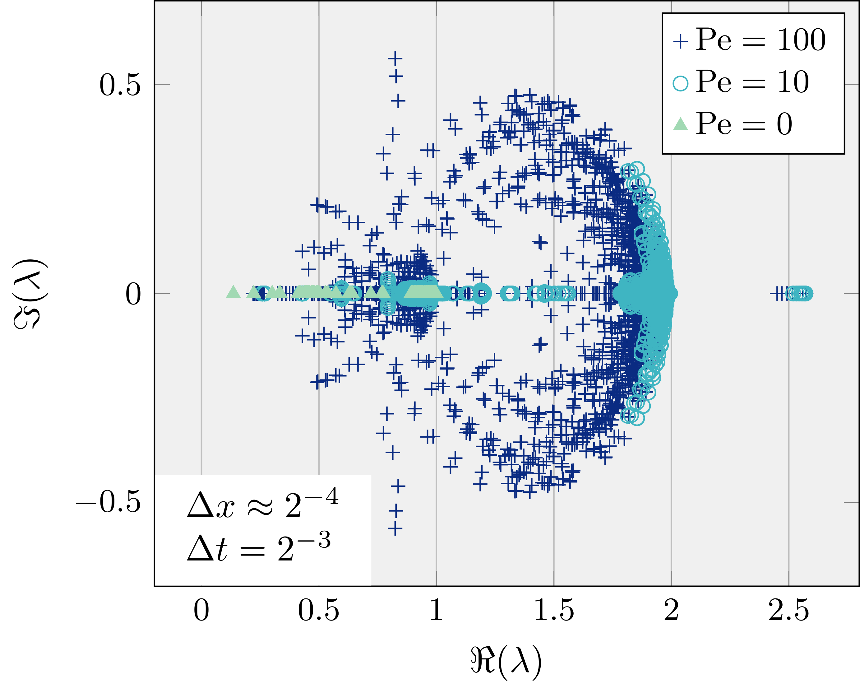
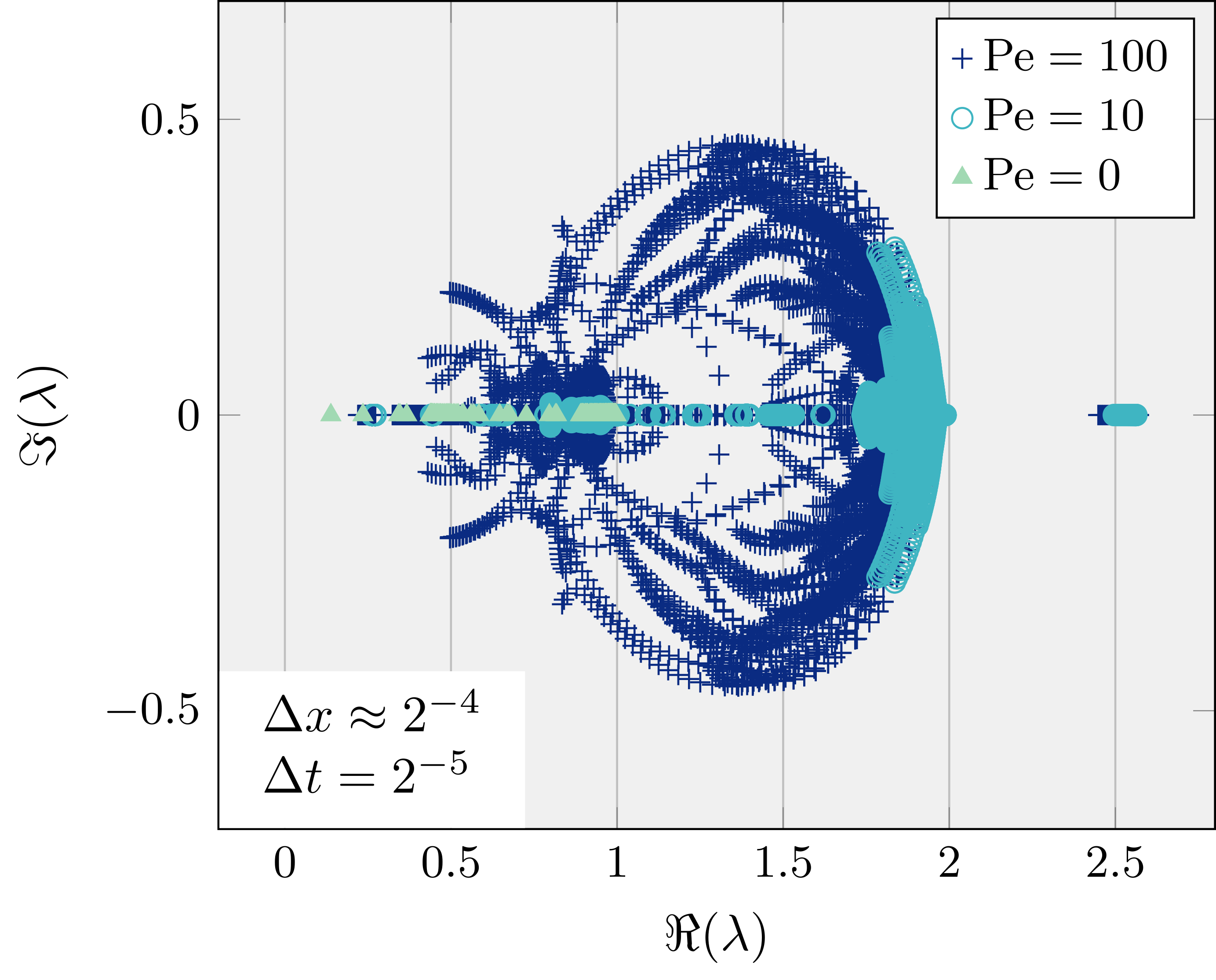
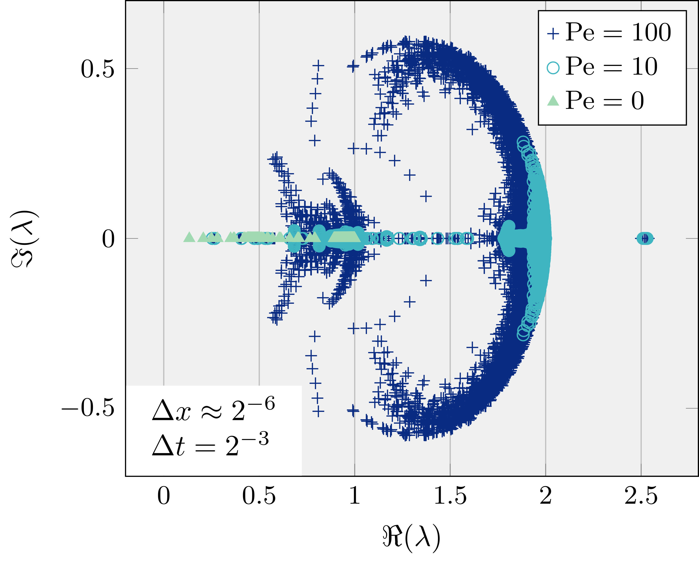
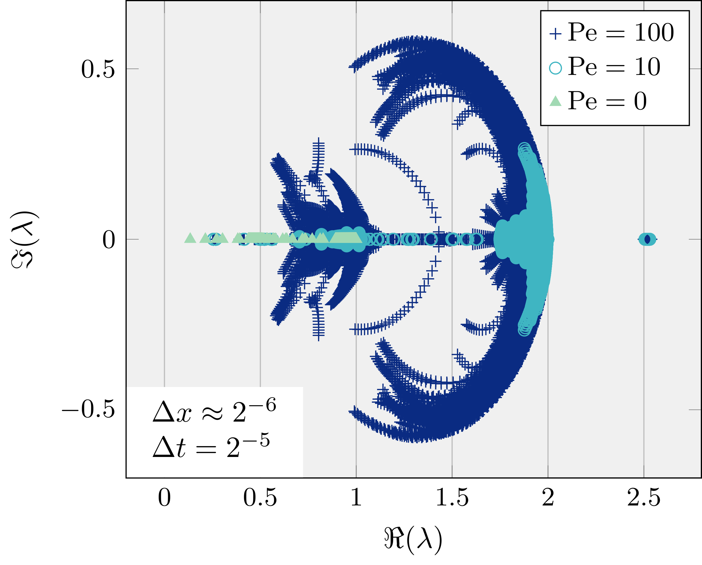
Figure 1: Eigenvalue distribution of the operators 59, corresponding to problem 4, for varying values of $\Delta t$, $\Delta x$, and Péclet number, Pe, which represents the intensity of the advection field. Here, Pe denotes the continuous Péclet number (i.e., not scaled by mesh spacing); see section 4.1 for its definition (notice choosing $\text{Pe}=0$ corresponds to problem 1). The eigenvalues are computed numerically using the MATLAB function eigs.

It is worth pointing out that increasing the Péclet number has the effect of pushing some eigenvalues towards $2$, and spreading more of them away from the real axis. It also makes the distributions more sensitive with respect to the level of refinement in the spatial discretisation, as can be seen comparing top and bottom plots in fig. 1: the dark blue tokens become more orderly distributed as $\Delta x$ decreases. These considerations makes us wary of a possible degradation in the performance of the preconditioner as advection becomes predominant, an issue that is observed and discussed in section 4.2.2. In general, however, most of the eigenvalues remain clustered inside $[0.1,2]\times[-0.6,0.6]$ in the complex plane.

4 Results

To demonstrate the performance of the preconditioner introduced in section 3, we consider its application for the solution of a variety of flow configurations. For simplicity, we focus on problems defined on $\Omega\subset\mathbb{R}^{2}$, although we point out that the applicability of 23 is by no means limited to 2D simulations. The test-cases hereby proposed have been adapted from problems used extensively in the literature (see for example [5, Chap. 3.1 and Chap. 6.1]), and are briefly described in section 4.1. The experiments conducted provide evidence for the optimal scalability of 23, as well as its potential for speed-up via time-parallelisation. Additionally, we investigate simple extensions to more general frameworks, such as the solution of nonlinear incompressible flow, and its applicability in advection-dominated regimes.

4.1 Model problems

The first three problems described in this section are test-cases for the time-dependent Stokes equations 2, while the last one is designed for Oseen 1. They are defined as follows.

1. Driven cavity flow. This represents a fully enclosed flow, defined on a square spatial domain ${\boldsymbol{x}}=(x,y)^{T}\in[0,1]^{2}\eqqcolon\Omega_{\square}$. No forcing term is considered, and homogeneous Dirichlet BC are imposed on the bottom, left and right sides of the domain. To accelerate the flow, we prescribe the velocity on the top side

   $${\boldsymbol{u}}_{C}({\boldsymbol{x}}|_{y=1},t)=8tx(1-x)(2x^{2}-2x+1).$$ (60)

   This profile is regularised so as to smoothly match the BC on the left and right sides. Notice that, in order to introduce time-dependency, the velocity is ramped up linearly from a quiet state: this is done in the following test-cases as well. An example solution for this problem is shown in fig. 2.

   

   

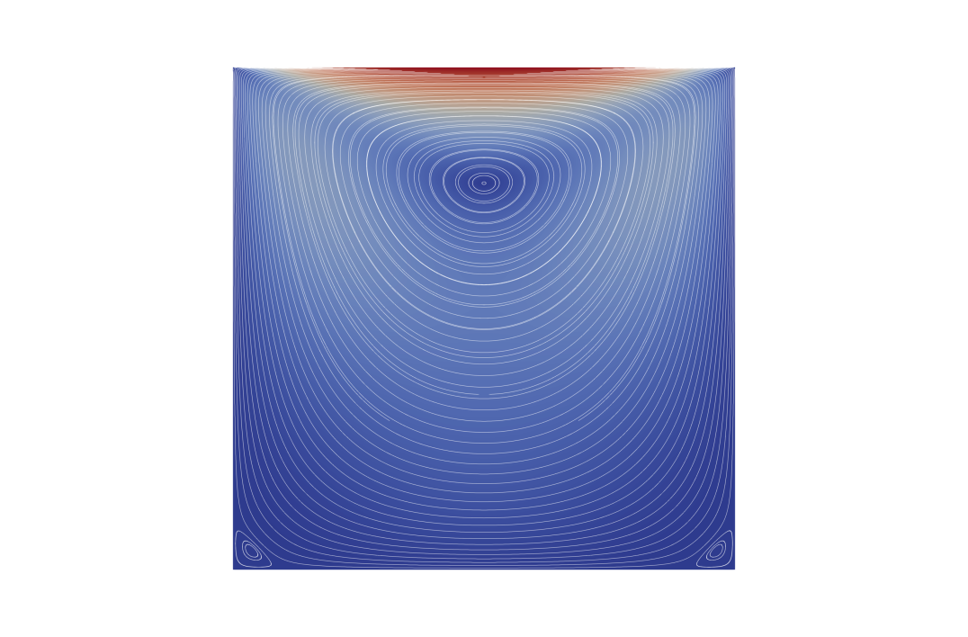
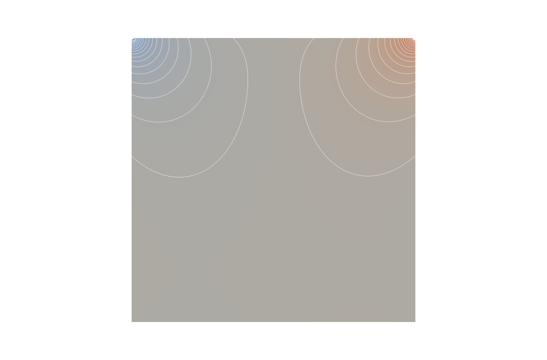
   Figure 2: Velocity magnitude and streamlines (left), and pressure contour plot (right) for an example solution of the driven cavity flow problem 1.

2. Poiseuille flow. Also defined on $\Omega_{\square}$, this set-up models laminar flow along a channel, for which the following analytical solution can be recovered:

   $${\boldsymbol{u}}_{P}({\boldsymbol{x}},t)=4t\left[\begin{array}[]{c}y(1-y)\\ 0\end{array}\right],\quad p_{P}({\boldsymbol{x}},t)=8(1-x).$$ (61)

   

   

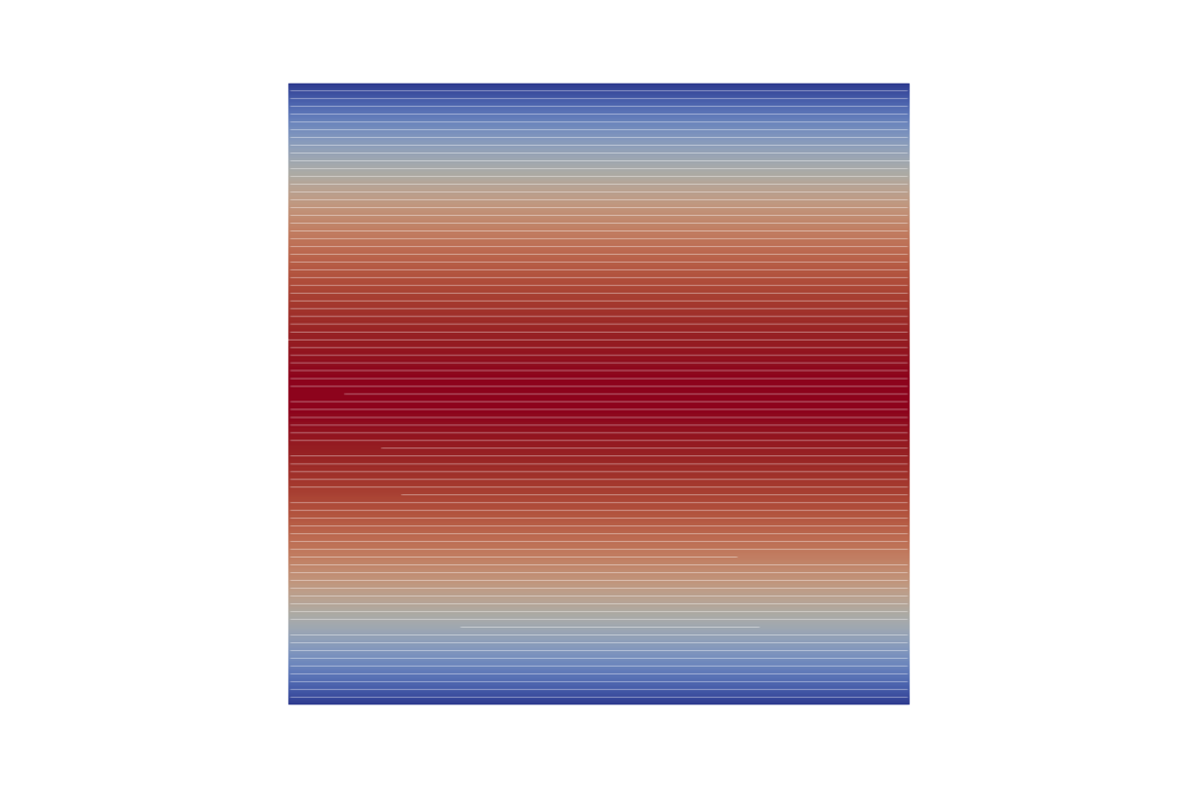
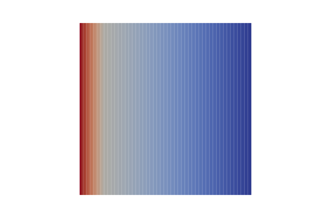
   Figure 3: Velocity magnitude and streamlines (left), and pressure contour plot (right) for the analytical solution of the Poiseuille flow problem 2.

   The forcing term is defined so as to counterbalance the time-derivative: $\boldsymbol{f}_{P}=4[y(1-y),0]^{T}$. No-slip conditions are included in the top and bottom sides of the channel, and a parabolic inflow profile is prescribed at $x=0$. At the outflow $x=1$, homogeneous Neumann BC are imposed. The analytical solution is plotted in fig. 3.

3. Flow over backward-facing step. This is another example of flow through a channel, except the fluid undergoes a sudden expansion. The domain is a stretched L-shape, $\Omega_{L}=[0,8]\times[0,1]\cup[1,8]\times[0,-1]$, and the BC imposed are similar to those for Poiseuille (the inflow, where the parabolic velocity profile is prescribed, is on the side $x=0$). As for problem 1, no forcing term is included; an example solution is provided in fig. 4.

   

   

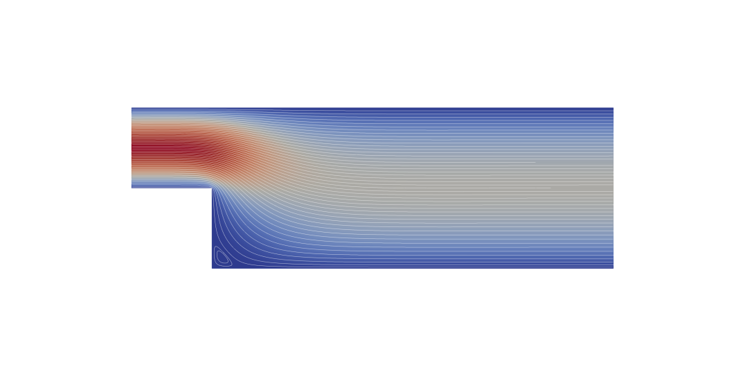
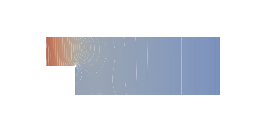
   Figure 4: Velocity magnitude and streamlines (top), and pressure contour plot (bottom) for an example solution of the flow over backward-facing step problem 3.

4. Double-glazing. The set-up for this problem is analogous to that of the driven cavity flow, except now the effect of a recirculating wind is included in the system:

   $${\boldsymbol{w}}_{G}({\boldsymbol{x}},t)=2t\left[\begin{array}[]{r}-(2y-1)(4x^{2}-4x+1)\\ (2x-1)(4y^{2}-4y+1)\end{array}\right]\mu\text{Pe},$$ (62)

   whose intensity can be adjusted by tweaking the value of the Péclet number Pe [30, Chap. 13.2]. This parameter describes the relative intensity of advective transport with respect to diffusive transport, and for a generic advection field ${\boldsymbol{w}}({\boldsymbol{x}},t)$ it can be defined as

   $$\text{Pe}\coloneqq\frac{LU}{\mu}=\frac{L}{\mu}\left(\frac{1}{T-T_{0}}\int_{T_{0}}^{T}\max_{{\boldsymbol{x}}\in\Omega}{\boldsymbol{w}}({\boldsymbol{x}},t)\,dt\right),$$ (63)

   where $L$ is a characteristic length of the spatial domain ($L=1$ for this problem), and $U$ a characteristic speed (considered averaged over the temporal domain). The impact that the added advection field has on the solution is illustrated in fig. 5.

   

   

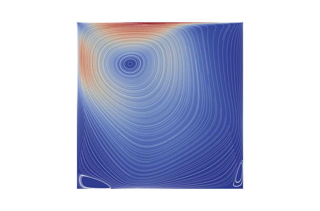
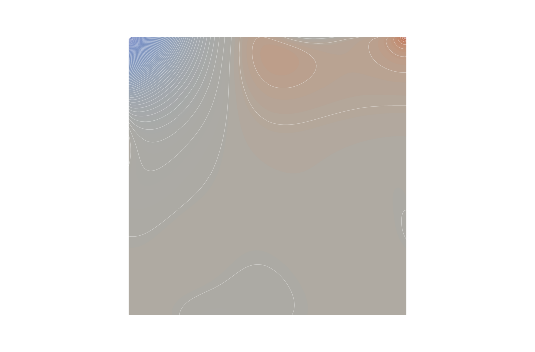
   Figure 5: Velocity magnitude and streamlines (left), and pressure contour plot (right) for an example solution of the double-glazing flow problem 4 with $\text{Pe}=10$.

For each test-case the temporal domain is given by $t\in[0,1]$, and the viscosity parameter is fixed to $\mu=1$. The discrete functional spaces are approximated using Taylor-Hood finite elements: $P_{2}$ for velocity and $P_{1}$ for pressure [30, Chap. 17.4], both defined on a triangular mesh. The code developed for our experiments is publicly available at the repository [4]. It makes use of the MFEM finite element package [26] for the assembly of the finite element matrices, and we rely on the PETSc [1] and hypre [18] implementations of the various solvers used. Unless otherwise specified, the space-time initial guess for the GMRES iterations is null (apart from the Dirichlet nodes, where we substitute the given data), although preliminary experiments with a random initial guess (uniformly distributed in $\left[-1,1\right]$) show negligible sensitivity of the convergence behaviour to this choice.

4.2 Performance of preconditioner

In this section, we conduct a series of experiments aimed at measuring the effectiveness of the proposed preconditioner 23 in accelerating GMRES. We chose the total number of iterations to convergence as the main measure of performance. The reason behind this preference (rather than, for example, computational time), lies in the fact that we believe it provides a more indicative metric for assessing the efficacy of our preconditioning strategy. This is in fact less dependent on the details of the actual implementation of the underlying solvers, and particularly of the one for the space-time velocity block 22, the optimal design of which is beyond the purpose of this manuscript: indeed a key point of our approach is the flexibility it provides in choosing such a solver.

4.2.1 Exact versus approximate solvers

As a first experiment, we test directly the application of our preconditioner to the solution of the model problems introduced in section 4.1. We provide two different set-ups for the solvers involved in the application of 23: an ideal one, in which we make use of exact solvers, in order to provide a best-case scenario for the performance of such preconditioner; and an approximate case, which instead gives us a measure of the performance degradation we can expect by applying iterative solvers instead of exact solvers, which is more realistic in practice.

Table 1: Number of GMRES iterations to $10^{-10}$ residual tolerance, when applied to the monolithic space-time system 21 right-preconditioned with $P_{T}^{-1}$ 23. Different levels of refinement are considered both for the spatial (rows) and temporal meshes (columns). The four sets of results refer to the four test problems introduced in section 4.1 (problem 4 has Péclet number $\text{Pe}=10$). Results on the left of each column are recovered using exact solvers, and results on the right of each column (in brackets) are recovered using approximate iterative solvers (inversion of ${\mathcal{M}}_{p}$ is approximated with 8 Jacobi-preconditioned Chebyshev iterations, inversion of ${\mathcal{A}}_{p}$ is approximated using 15 iterations of AMG, and the solution of the space-time velocity block $F_{{\boldsymbol{u}}}$ is recovered applying 15 iterations of GMRES preconditioned by AIR). The outer solver in the latter case is FGMRES. Crosses identify crashing simulations (due to memory requirements becoming too severe).

Pb	${\begin{array}[]{@{}r@{}}\scriptstyle\Delta t\smash{\eqmakebox[ind]{$\scriptstyle\rightarrow$}}\\[-3.0pt] \scriptstyle\Delta x\smash{\eqmakebox[ind]{$\scriptstyle\downarrow$}}\end{array}}$	$2^{-1}$		$2^{-2}$		$2^{-3}$		$2^{-4}$		$2^{-5}$		$2^{-6}$		$2^{-7}$
1	$2^{-2}$	$23$	$(23)$	$24$	$(24)$	$25$	$(25)$	$26$	$(26)$	$25$	$(25)$	$26$	$(26)$	$26$	$(26)$
	$2^{-3}$	$22$	$(22)$	$22$	$(22)$	$23$	$(23)$	$24$	$(26)$	$24$	$(26)$	$24$	$(24)$	$25$	$(25)$
	$2^{-4}$	$22$	$(22)$	$22$	$(22)$	$23$	$(23)$	$23$	$(22)$	$22$	$(22)$	$23$	$(31)$	$22$	$(28)$
	$2^{-5}$	$20$	$(20)$	$21$	$(21)$	$21$	$(21)$	$20$	$(20)$	$20$	$(20)$	$20$	$(28)$	$20$	$(21)$
	$2^{-6}$	$19$	$(19)$	$19$	$(19)$	$19$	$(18)$	$19$	$(19)$	$19$	$(18)$	$19$	$(19)$	$20$	$(20)$
	$2^{-7}$	$18$	$(18)$	$18$	$(18)$	$19$	$(18)$	$18$	$(18)$	$19$	$(19)$	$18$	$(18)$	$19$	$(19)$
	$2^{-8}$	$17$	$(17)$	$18$	$(18)$	$18$	$(17)$	$17$	$(17)$	$18$	$(18)$	$17$	$(17)$	$16$	$(17)$
2	$2^{-2}$	$28$	$(28)$	$32$	$(32)$	$34$	$(34)$	$36$	$(36)$	$40$	$(40)$	$43$	$(43)$	$49$	$(50)$
	$2^{-3}$	$31$	$(31)$	$34$	$(34)$	$35$	$(35)$	$36$	$(41)$	$38$	$(42)$	$39$	$(38)$	$38$	$(39)$
	$2^{-4}$	$30$	$(30)$	$32$	$(32)$	$33$	$(33)$	$34$	$(34)$	$34$	$(36)$	$35$	$(49)$	$35$	$(44)$
	$2^{-5}$	$29$	$(29)$	$31$	$(30)$	$32$	$(32)$	$33$	$(33)$	$34$	$(35)$	$34$	$(49)$	$34$	$(37)$
	$2^{-6}$	$28$	$(28)$	$30$	$(30)$	$31$	$(31)$	$32$	$(32)$	$32$	$(32)$	$33$	$(34)$	$31$	$(32)$
	$2^{-7}$	$27$	$(27)$	$29$	$(28)$	$30$	$(30)$	$30$	$(30)$	$30$	$(30)$	$29$	$(30)$	$29$	$(30)$
	$2^{-8}$	$25$	$(25)$	$26$	$(26)$	$27$	$(26)$	$28$	$(27)$	$26$	$(26)$	$26$	$(27)$	$26$	$(27)$
3	$2^{-2}$	$33$	$(34)$	$35$	$(40)$	$37$	$(42)$	$38$	$(38)$	$42$	$(42)$	$46$	$(46)$	$53$	$(55)$
	$2^{-3}$	$33$	$(33)$	$35$	$(35)$	$36$	$(37)$	$37$	$(49)$	$39$	$(47)$	$39$	$(39)$	$40$	$(40)$
	$2^{-4}$	$31$	$(31)$	$33$	$(33)$	$34$	$(34)$	$35$	$(47)$	$35$	$(38)$	$36$	$(53)$	$37$	$(48)$
	$2^{-5}$	$30$	$(30)$	$32$	$(32)$	$33$	$(33)$	$34$	$(34)$	$34$	$(35)$	$36$	$(53)$	$35$	$(39)$
	$2^{-6}$	$28$	$(28)$	$31$	$(31)$	$32$	$(32)$	$32$	$(32)$	$33$	$(33)$	$33$	$(34)$	$33$	$(35)$
	$2^{-7}$	$27$	$(27)$	$29$	$(29)$	$30$	$(30)$	$31$	$(31)$	$31$	$(31)$	$30$	$(30)$	$30$	$(30)$
	$2^{-8}$	$25$	$(26)$	$27$	$(27)$	$28$	$(28)$	$28$	$(28)$	$28$	$(28)$	$26$	$(27)$	$\times$	$(\times)$
4	$2^{-2}$	$25$	$(25)$	$27$	$(27)$	$27$	$(27)$	$27$	$(27)$	$28$	$(28)$	$27$	$(27)$	$27$	$(27)$
	$2^{-3}$	$24$	$(24)$	$25$	$(25)$	$25$	$(25)$	$26$	$(28)$	$26$	$(27)$	$26$	$(26)$	$26$	$(26)$
	$2^{-4}$	$24$	$(24)$	$25$	$(25)$	$25$	$(25)$	$25$	$(26)$	$24$	$(25)$	$24$	$(31)$	$23$	$(28)$
	$2^{-5}$	$24$	$(24)$	$24$	$(26)$	$23$	$(25)$	$23$	$(24)$	$22$	$(24)$	$23$	$(32)$	$22$	$(24)$
	$2^{-6}$	$21$	$(23)$	$22$	$(25)$	$22$	$(26)$	$21$	$(26)$	$21$	$(26)$	$22$	$(28)$	$21$	$(28)$
	$2^{-7}$	$20$	$(24)$	$21$	$(26)$	$21$	$(28)$	$20$	$(28)$	$21$	$(31)$	$21$	$(32)$	$20$	$(33)$
	$2^{-8}$	$19$	$(24)$	$20$	$(27)$	$20$	$(28)$	$19$	$(30)$	$20$	$(32)$	$19$	$(32)$	$19$	$(34)$

In more detail, the application of the inverse of 23 involves inverting three different operators: two of these are associated with the application of the approximate space-time Schur complement 37, and require inverting the pressure mass matrix ${\mathcal{M}}_{p}$ 29a, and the pressure “Laplacian” $\tilde{{\mathcal{A}}}_{p}$ 35; the last one must deal with the monolithic space-time matrix for the velocity variable $F_{\boldsymbol{u}}$ 22. In the ideal case, we exploit LU solvers for both 29a and 35, and a sequential time-stepping procedure for 22 (the latter further requires inverting the spatial velocity operator ${\mathcal{F}}_{{\boldsymbol{u}},k}$ 17 at each time-step $k$, for which we also use LU).

However, resorting to direct methods becomes infeasible when solving systems of large size, both in terms of memory and of computations required. Moreover, our final goal is to actually parallelise in time the solution of the monolithic system. In order to do so, we must substitute the time-stepping procedure for the space-time velocity block $F_{{\boldsymbol{u}}}$ with a parallel alternative. Here, we use GMRES preconditioned by nonsymmetric AMG based on approximate ideal restriction (AIR) [24, 23], as implemented in hypre. AIR was designed as a reduction-based classical AMG solver for advection-dominated problems, but was shown to be effective on advection-diffusion problems as well. More recently, AIR was demonstrated as an effective algebraic solver for space-time finite element discretisations of advection(-diffusion) [37]. Although likely not as effective as space-time geometric multigrid techniques (e.g., [17]) for diffusive problems, AIR is likely more robust for advective regimes and also less intrusive to apply, as we simply need to form the space-time velocity matrix and pass it to hypre. Due to the use of an inner Krylov method, we swap the outer GMRES solver with a flexible-GMRES (FGMRES) solver [34]. The inversions of the pressure mass and stiffness matrices are also approximated: for ${\mathcal{M}}_{p}$, we apply a fixed number of Chebyshev iterations [43], making use of the bounds on its eigenvalues provided by [44]; for $\tilde{{\mathcal{A}}}_{p}$, we apply hypre’s BoomerAMG [33].

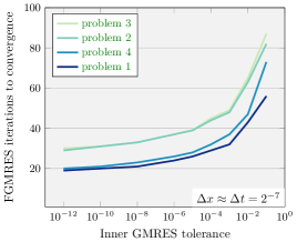
Figure 6: Number of outer FGMRES iterations to convergence for different tolerances of the inner GMRES solver for the space-time velocity block $F_{\boldsymbol{u}}$ in 23. The discretisation parameters are fixed to $\Delta x\approx\Delta t=2^{-7}$ for all problems in section 4.1. The remaining options for the solvers involved are the same ones used to fill the right column in table 1.

Results from using direct or approximate solvers are reported side-by-side in table 1, for ease of comparison. The two cases show a remarkably similar convergence behaviour, with the total number of iterations to convergence remaining substantially unchanged. The only notable disparities are observed for the most complex problem 4, likely because the 15 AIR iterations used as an approximate solver for the space-time velocity block do not provide as accurate of an approximation as for problems 1, 2, and 3. Even here, the increase in iterations compared with exact inner solves is nicely bounded, remaining below a factor of $2$ with respect to the ideal case. This shows that the approximate solvers employed can be as effective as their direct counterparts, and gives an example of an effective time-parallel procedure which can work well in tandem with the preconditioner proposed.

To draw a clearer picture of the sensitivity of our space-time block preconditioning procedure to the approximate solution of the velocity block, we analyse more in detail how the tolerance of the solver chosen for $F_{{\boldsymbol{u}}}$ impacts the total number of iterations to convergence for the outer solver. This gives some indication of the target accuracy required by the PinT solver for the space-time block preconditioner to still be effective. From the results shown in fig. 6, it transpires that we can afford solving the space-time velocity system with a tolerance as lax as $\approx 10^{-3}$, and still retain convergence with a reasonably small number of iterations. Remarkably, this is in line with the required tolerance for the velocity block solve ${\mathcal{F}}_{{\boldsymbol{u}},k}$ in the single time-step preconditioner 41 as observed, for example, in [38].

We point out that, for the largest problems considered, the relevant systems have sizes $N_{u}=526,338$, $N_{p}=66,049$, and $N_{t}=128$, for a total number of unknowns of $(N_{u}+N_{p})\cdot N_{t}\approx 76\cdot 10^{6}$; this further increases to $N_{u}=5,775,362$, $N_{p}=722,945$, and $N_{t}=64$, totalling $\approx 416\cdot 10^{6}$, for problem 3 (a simulation with $\approx 832\cdot 10^{6}$ degrees of freedom crashed due to lack of memory). Compared to the noticeable size of the system, the total number of iterations to convergence reported in table 1 remains small, regardless of mesh size and problem type, providing evidence of the optimal scalability of the preconditioners proposed. This is further confirmed by tracking more in detail the evolution of the residual as the GMRES iterations progress: an example of this is provided in fig. 7, which shows reasonably uniform convergence profiles, independently of the choice of both $\Delta x$ and $\Delta t$.

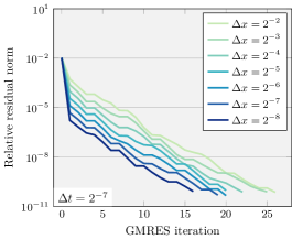
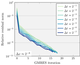
Figure 7: Details on relative (with respect to the norm of the right-hand side) residual evolution of GMRES applied to problem 1, using $P_{T}^{-1}$ with ideal components as a right-preconditioner. Results on the left refer to simulations with fixed $\Delta t=2^{-7}$ and varying $\Delta x$; results on the right are obtained by fixing $\Delta x\approx 2^{-8}$ and varying $\Delta t$. The set-up for the solvers is similar to the one used for table 1.

4.2.2 Dependence on Péclet number

Table 2: Number of iterations to convergence for problem 4 with different values of Pe. Dashes represent simulations that did not converge in the maximum prescribed number of iterations ($100$). Same solvers set-up as for the ideal case in table 1.

${\begin{array}[]{@{}r@{}}\scriptstyle\Delta t\smash{\eqmakebox[ind]{$\scriptstyle\rightarrow$}}\\[-3.0pt] \scriptstyle\Delta x\smash{\eqmakebox[ind]{$\scriptstyle\downarrow$}}\end{array}}$	$2^{-4}$					$2^{-5}$					$2^{-6}$					$2^{-7}$
Pe$\to$	$2^{4}$	$2^{5}$	$2^{6}$	$2^{7}$	$2^{8}$	$2^{4}$	$2^{5}$	$2^{6}$	$2^{7}$	$2^{8}$	$2^{4}$	$2^{5}$	$2^{6}$	$2^{7}$	$2^{8}$	$2^{4}$	$2^{5}$	$2^{6}$	$2^{7}$	$2^{8}$
$2^{-2}$	$32$	$60$	$//$	$//$	$//$	$32$	$57$	$//$	$//$	$//$	$31$	$55$	$//$	$//$	$//$	$31$	$54$	$//$	$//$	$//$
$2^{-3}$	$28$	$35$	$54$	$//$	$//$	$28$	$35$	$53$	$//$	$//$	$28$	$35$	$53$	$//$	$//$	$27$	$35$	$52$	$//$	$//$
$2^{-4}$	$27$	$32$	$40$	$55$	$//$	$27$	$32$	$39$	$55$	$//$	$25$	$31$	$38$	$53$	$//$	$25$	$31$	$38$	$52$	$//$
$2^{-5}$	$25$	$30$	$35$	$45$	$66$	$25$	$28$	$35$	$44$	$66$	$24$	$28$	$34$	$44$	$64$	$23$	$27$	$34$	$43$	$63$
$2^{-6}$	$24$	$27$	$32$	$39$	$49$	$23$	$27$	$32$	$38$	$49$	$23$	$27$	$32$	$37$	$48$	$22$	$26$	$30$	$37$	$47$
$2^{-7}$	$23$	$26$	$31$	$35$	$40$	$22$	$26$	$30$	$35$	$41$	$22$	$26$	$29$	$33$	$41$	$21$	$25$	$29$	$33$	$40$
$2^{-8}$	$22$	$25$	$29$	$32$	$37$	$21$	$25$	$29$	$32$	$37$	$21$	$25$	$28$	$32$	$37$	$20$	$24$	$27$	$32$	$37$

When applied to the solution of Oseen equations, we observe that the performance of the preconditioner degrades as we increase the intensity of the advection field imposed, as foreshadowed by the analysis in section 3.3. This is shown in table 2, where we progressively ramp up the value of Pe in problem 4, solving for various $\Delta x$: convergence fails for coarser spatial meshes and largest Péclet numbers. This hints at the necessity of either employing appropriately refined meshes, or relying on stabilisation techniques [30, Chap. 13.8] (which we did not apply in our analysis), whenever advection-dominated flows need to be resolved. The preconditioner for the single time-step case 41 was shown to suffer from a similar lack of robustness [5, Table 9.3], so it is somewhat expected that this weakness carries over to the whole space-time case. However, we point out that the performance of the preconditioner does not vary significantly as long as we keep constant the grid Péclet number $\tilde{\text{Pe}}\coloneqq\Delta x\text{Pe}/L$ [30, Chap. 13.2]. Unlike its global counterpart 63, this parameter provides a local measure of the dominance of advection over diffusion, and is useful in identifying conditions for which instabilities and oscillations might arise in the numerical solution. This parameter is kept fixed down each diagonal of table 2, which show only slow growth in the number of iterations to convergence with increasing Pe.

4.3 The nonlinear setting: incompressible Navier-Stokes

As stated in section 2, Oseen equations 1 can be interpreted as a linearisation of the Navier-Stokes system 3. If we then introduce an outer solver to tackle the nonlinear advection term in Navier-Stokes, we can use our preconditioner to accelerate the solution of the corresponding inner (linearised) problems, much like what is done for the single time-step case in [5, Chap. 10]. We experiment on the performance of our preconditioner $P_{T}$ 23 in this situation, and resolve the nonlinearity in 3 via Picard iterations [29]. That is, we iteratively solve the linearised system

$$\left[\begin{array}[]{c|c}F_{{\boldsymbol{u}}}(({\boldsymbol{u}})^{j})&B^{T}\rule[-3.87495pt]{0.0pt}{0.0pt}\\ \hline\cr B&\mathbf{0}\rule{0.0pt}{11.19443pt}\end{array}\right]\left[\begin{array}[]{c}({\boldsymbol{u}})^{j+1}\rule[-3.87495pt]{0.0pt}{0.0pt}\\ \hline\cr({\boldsymbol{p}})^{j+1}\rule{0.0pt}{11.19443pt}\end{array}\right]=\left[\begin{array}[]{c}{\boldsymbol{f}}\rule[-3.87495pt]{0.0pt}{0.0pt}\\ \hline\cr{\boldsymbol{0}}\rule{0.0pt}{11.19443pt}\end{array}\right],$$ (64)

until convergence is reached. Here, $({\boldsymbol{u}})^{j+1}$ and $({\boldsymbol{p}})^{j+1}$ denote the whole space-time velocity and pressure solutions at the $j+1$-th Picard iteration, while we made explicit the dependence of the space-time velocity block $F_{{\boldsymbol{u}}}=F_{{\boldsymbol{u}}}({\boldsymbol{w}})$ on the advection field, which we substitute with the approximate solution at the previous iteration $({\boldsymbol{u}})^{j}$.

Table 3: Convergence results for Navier-Stokes with the setup of problems 1 and 3. Picard iterations used as the outer nonlinear solver, which achieves convergence with a tolerance of $10^{-9}$. Inside each column, on the left is reported the number of outer iterations to convergence, while on the right (in brackets) the average number of inner GMRES iterations per outer Picard iteration. The inner GMRES solver has the options used for recovering the results in the left column of table 1. Notice problem 2 is missing: this is because the nonlinearity does not affect the analytical solution for Poiseuille, and hence results are not particularly informative in this case (convergence occurs at the very first Picard iteration in almost the totality of the experiments). Also problem 4 is missing, since it already represents a linearisation of Navier-Stokes for problem 1. Crosses identify crashing simulations (due to memory requirements becoming too severe).

Pb	${\begin{array}[]{@{}r@{}}\scriptstyle\Delta t\smash{\eqmakebox[ind]{$\scriptstyle\rightarrow$}}\\[-3.0pt] \scriptstyle\Delta x\smash{\eqmakebox[ind]{$\scriptstyle\downarrow$}}\end{array}}$	$2^{-1}$		$2^{-2}$		$2^{-3}$		$2^{-4}$		$2^{-5}$		$2^{-6}$		$2^{-7}$
1	$2^{-2}$	$5$	$(11.60)$	$4$	$(14.75)$	$4$	$(14.25)$	$4$	$(14.50)$	$4$	$(13.50)$	$4$	$(13.25)$	$4$	$(13.00)$
	$2^{-3}$	$4$	$(13.50)$	$4$	$(13.25)$	$4$	$(13.25)$	$4$	$(13.00)$	$4$	$(12.50)$	$4$	$(12.25)$	$5$	$(9.40)$
	$2^{-4}$	$4$	$(12.50)$	$4$	$(12.50)$	$4$	$(12.25)$	$4$	$(12.00)$	$4$	$(11.50)$	$5$	$(8.80)$	$5$	$(8.60)$
	$2^{-5}$	$4$	$(11.50)$	$4$	$(11.00)$	$4$	$(11.50)$	$4$	$(10.75)$	$5$	$(8.00)$	$5$	$(8.20)$	$4$	$(9.25)$
	$2^{-6}$	$4$	$(10.50)$	$4$	$(10.00)$	$4$	$(10.00)$	$4$	$(9.50)$	$4$	$(9.25)$	$4$	$(8.50)$	$4$	$(8.75)$
	$2^{-7}$	$4$	$(9.75)$	$4$	$(9.00)$	$4$	$(9.25)$	$5$	$(6.80)$	$4$	$(8.25)$	$4$	$(8.00)$	$4$	$(7.75)$
	$2^{-8}$	$3$	$(11.00)$	$3$	$(11.00)$	$3$	$(10.67)$	$3$	$(10.33)$	$3$	$(10.33)$	$4$	$(7.25)$	$4$	$(6.75)$
3	$2^{-2}$	$5$	$(19.80)$	$5$	$(18.20)$	$5$	$(18.00)$	$5$	$(18.00)$	$5$	$(18.40)$	$5$	$(19.00)$	$5$	$(21.40)$
	$2^{-3}$	$5$	$(21.80)$	$5$	$(19.60)$	$5$	$(17.80)$	$5$	$(17.00)$	$5$	$(16.80)$	$5$	$(16.40)$	$5$	$(16.20)$
	$2^{-4}$	$5$	$(22.60)$	$5$	$(20.60)$	$5$	$(18.80)$	$5$	$(16.80)$	$5$	$(15.60)$	$5$	$(14.80)$	$5$	$(14.20)$
	$2^{-5}$	$5$	$(26.60)$	$5$	$(22.80)$	$5$	$(20.60)$	$5$	$(17.60)$	$5$	$(16.20)$	$5$	$(15.80)$	$5$	$(14.20)$
	$2^{-6}$	$4$	$(36.00)$	$4$	$(31.75)$	$4$	$(28.25)$	$5$	$(18.00)$	$5$	$(17.20)$	$5$	$(16.00)$	$5$	$(14.80)$
	$2^{-7}$	$4$	$(43.00)$	$4$	$(37.00)$	$4$	$(31.75)$	$4$	$(24.75)$	$5$	$(18.40)$	$5$	$(18.60)$	$5$	$(15.00)$
	$2^{-8}$	$4$	$(52.50)$	$4$	$(46.25)$	$4$	$(33.50)$	$4$	$(28.25)$	$5$	$(22.40)$	$\times$	$(\times)$	$\times$	$(\times)$

Linear and nonlinear convergence obtained by applying a Picard linearisation 64 to the problems in section 4.1 are reported in table 3. Especially for problem 1, both the inner and outer solve iterations remain $\mathcal{O}(1)$, independently on the spatial and temporal mesh spacing. Similar results holds for the inflow-outflow problem problem 3, but here the average number of inner GMRES iterations is larger. In the specific case of a very large time-step relative to the spatial mesh, the number of inner iterations can be a fair amount larger. However, this is not necessarily surprising, as problem 3 offers more complex dynamical behavior and we are resolving the nonlinearity over a very large time-step. This likely results in a very stiff and ill-conditioned linear system to solve for each nonlinear iteration. Nevertheless, the outer space-time Picard linearisation remains perfectly scalable.

4.4 Comparison with sequential time-stepping

Section 3.1.1 explains how the two main factors in analysing the effectiveness of our preconditioning strategy compared with classical time-stepping are given by the ratios $C_{F_{{\boldsymbol{u}}}}/(C_{{\mathcal{F}}_{{\boldsymbol{u}}}}\,N_{t})$ and $N_{it}^{ST}/N_{it}^{0}$. The first ratio directly refers to the efficiency of the method chosen for the parallel-in-time integration of the velocity block $F_{{\boldsymbol{u}}}$: identifying the optimal solver in this sense is still a matter of research, and a detailed investigation comparing the effectiveness of the various parallel-in-time methods available in the literature [11] goes well beyond the scope of this paper. Here, we focus on the second ratio because it is intrinsic to the preconditioning strategy proposed: in fact, it describes the overhead produced by tackling the whole space-time system at once, rather than via sequential time-stepping.

Table 4: Ratio $N_{it}^{ST}/N_{it}^{0}$, where $N_{it}^{ST}$ is taken from the ideal case in table 1, while $N_{it}^{0}$ represents the average number of iterations to convergence per time-step, solving for 18 via forward substitution. For the latter, GMRES is used at each time-step, right-preconditioned with the single time-step counterpart of $P_{T}$, 41 with 42. Convergence is reached with a tolerance of $10^{-10}/\sqrt[]{N_{t}}$. The remaining options for the solvers involved are the same ones used to fill the left column in table 1. Crosses identify crashing simulations (due to memory requirements becoming too severe).

Pb	${\begin{array}[]{@{}r@{}}\scriptstyle\Delta t\smash{\eqmakebox[ind]{$\scriptstyle\rightarrow$}}\\[-3.0pt] \scriptstyle\Delta x\smash{\eqmakebox[ind]{$\scriptstyle\downarrow$}}\end{array}}$	$2^{-2}$	$2^{-3}$	$2^{-4}$	$2^{-5}$	$2^{-6}$	$2^{-7}$	$2^{-2}$	$2^{-3}$	$2^{-4}$	$2^{-5}$	$2^{-6}$	$2^{-7}$	Pb
1	$2^{-2}$	$1.17$	$1.32$	$1.33$	$1.39$	$1.58$	$1.78$	$1.39$	$1.55$	$1.76$	$2.11$	$2.43$	$2.98$	3
	$2^{-3}$	$1.02$	$1.08$	$1.23$	$1.45$	$1.60$	$1.74$	$1.28$	$1.42$	$1.64$	$1.81$	$2.00$	$2.27$
	$2^{-4}$	$1.02$	$1.16$	$1.30$	$1.33$	$1.46$	$1.51$	$1.21$	$1.31$	$1.44$	$1.58$	$1.80$	$2.09$
	$2^{-5}$	$1.06$	$1.17$	$1.15$	$1.21$	$1.27$	$1.34$	$1.17$	$1.28$	$1.42$	$1.56$	$1.82$	$2.07$
	$2^{-6}$	$1.03$	$1.07$	$1.09$	$1.14$	$1.21$	$1.33$	$1.18$	$1.27$	$1.37$	$1.57$	$1.86$	$2.28$
	$2^{-7}$	$1.00$	$1.09$	$1.04$	$1.17$	$1.16$	$1.33$	$1.15$	$1.26$	$1.45$	$1.70$	$1.98$	$2.35$
	$2^{-8}$	$1.03$	$1.05$	$1.03$	$1.16$	$1.20$	$1.27$	$1.16$	$1.29$	$1.52$	$1.74$	$1.92$	$\times$
2	$2^{-2}$	$1.42$	$1.62$	$1.83$	$2.12$	$2.53$	$3.13$	$1.24$	$1.29$	$1.34$	$1.48$	$1.59$	$1.81$	4
	$2^{-3}$	$1.36$	$1.44$	$1.61$	$1.82$	$2.08$	$2.26$	$1.10$	$1.12$	$1.25$	$1.46$	$1.61$	$1.73$
	$2^{-4}$	$1.19$	$1.26$	$1.34$	$1.49$	$1.74$	$1.96$	$1.12$	$1.16$	$1.30$	$1.33$	$1.42$	$1.41$
	$2^{-5}$	$1.15$	$1.20$	$1.28$	$1.48$	$1.66$	$1.99$	$1.19$	$1.17$	$1.21$	$1.22$	$1.30$	$1.29$
	$2^{-6}$	$1.10$	$1.17$	$1.28$	$1.44$	$1.81$	$2.19$	$1.10$	$1.10$	$1.11$	$1.17$	$1.22$	$1.29$
	$2^{-7}$	$1.10$	$1.20$	$1.30$	$1.57$	$1.89$	$2.46$	$1.06$	$1.05$	$1.06$	$1.19$	$1.25$	$1.26$
	$2^{-8}$	$1.07$	$1.19$	$1.42$	$1.58$	$1.95$	$2.54$	$1.05$	$1.05$	$1.05$	$1.19$	$1.21$	$1.37$

To give an indication of how $N_{it}^{0}$ and $N_{it}^{ST}$ compare with each other when ideal solvers are employed, we collect convergence results from the application of 41 within the time-stepping procedure, for problems equivalent to those analysed in table 1. To render the comparison more fair, for the single time-step we ask for a stricter tolerance on convergence, scaled by a factor $\sqrt[]{N_{t}}$ with respect to the whole space-time case: in this way, the Euclidean norm of the final space-time residual is similar in the two cases. We report the resulting ratio $N_{it}^{ST}/N_{it}^{0}$ in table 4. We can see that this sits between roughly $1$ and $3$, in most cases closer to one, but becoming larger as $\Delta t\to 0$, particularly $\Delta t\ll\Delta x$. This observation can be explained by pointing out that most of the advantage of time-stepping is given by the fact that, at each iteration, a good initial guess is provided by the value of the solution at the previous time-step, which we exploit in our experiments: with a reduced step-size, it is safe to expect that also the solution varies less between one time-step and the next. Nevertheless, results demonstrate little-to-no degradation in convergence speed between the two approaches and, thus, minimal overhead in applying block preconditioning techniques in an all-at-once fashion, compared with sequential time-stepping.

5 Conclusion and future work

In this work, we introduce a novel all-at-once block preconditioner for the discretised time-dependent Oseen equations. We take inspiration from heuristics that have proven successful in the single time-step or steady-state settings, and apply similar principles to the space-time setting. The preconditioning procedure is designed to better expose the system to effective strategies for time-parallelisation by partitioning the preconditioning into two stages: (i) the space-time solution of a time-dependent advection-diffusion equation, and (ii) a (spatial) mass-matrix inverse and pressure Laplacian inverse at each time point. The latter can easily be applied in a fast parallel manner using existing methods and is nearly analogous to sequential time-stepping. Stage (i) reduces the solution of a space-time system of PDEs to the (approximate) solution of a single-variable space-time PDE, a much more tractable problem for fast, parallel solvers. In particular, a number of approaches have already seen success here, including space-time geometric multigrid [9, 17] and AMG applied to the space-time matrix [37], as well as the more standard PinT methods [11].

The approach pursued here provides a different take on time-parallelisation for time-dependent incompressible flows, compared with what is typically done in the literature [27, 41, 40, 3, 10]. To our knowledge, most of the latter leaves the underlying time-stepping procedure for solving 18 largely unchanged, and rather focuses on building an overarching framework which breaks its innate sequentiality. Instead, our method exploits the block structure of the system at the space-time level, in order to simplify the type of problem we need to (parallel-)integrate in time. We can draw an analogy between the role of the preconditioner for the single time-step case 41 and our space-time preconditioner 23: the first provides an effective method for solving Oseen via sequential time stepping, so long as a fast solver for an elliptic operator is available; the second provides an effective method for solving space-time Oseen, so long as a fast (time-parallel) solver for a parabolic operator is available.

The effectiveness of our preconditioner is demonstrated by applying it to a variety of model problems taken from the literature, which cover a range of flow configurations. The main measure for performance is given by the number of iterations required for convergence, which we have shown to be scalable in spatial and temporal mesh size, and comparable to those required for a classical time-stepping (non-time-parallel) routine. A simple extension to a nonlinear Navier-Stokes problem is investigated as well, which is linearised via a Picard iteration, wherein we observe near perfect scalability of linear and nonlinear iterations.

Future research will revolve around developing fast, robust, and time-parallel solution methods for the scalar space-time velocity block in our preconditioner, and extending the principles developed in this paper to the space-time solution of other time-dependent systems of PDEs.

References

- [1] S. Balay, S. Abhyankar, M. F. Adams, J. Brown, P. Brune, K. Buschelman, L. Dalcin, A. Dener, V. Eijkhout, W. D. Gropp, D. Karpeyev, D. Kaushik, M. G. Knepley, D. A. May, L. C. McInnes, R. T. Mills, T. Munson, K. Rupp, P. Sanan, B. F. Smith, S. Zampini, H. Zhang, and H. Zhang, PETSc Web page. https://www.mcs.anl.gov/petsc, 2019, https://www.mcs.anl.gov/petsc.
- [2] J. Cahouet and J.-P. Chabard, Some fast 3d finite element solvers for the generalized Stokes problem, International Journal for Numerical Methods in Fluids, 8 (1988), pp. 869–895, https://doi.org/10.1002/fld.1650080802.
- [3] R. Croce, D. Ruprecht, and R. Krause, Parallel-in-space-and-time simulation of the three-dimensional, unsteady Navier-Stokes equations for incompressible flow, in Modeling, Simulation and Optimization of Complex Processes-HPSC 2012, Springer, 2014, pp. 13–23, https://doi.org/10.1007/978-3-319-09063-4_2.
- [4] F. Danieli, STBP-incompressible-flow. https://gitlab.com/fdanieli/stbp-incompressible-flow, 2020.
- [5] H. Elman, D. Silvester, and A. Wathen, Finite Elements and Fast Iterative Solvers: with Applications in Incompressible Fluid Dynamics, Numerical Mathematics and Scientific Computation, Oxford University Press, 2014, https://doi.org/10.1093/acprof:oso/9780199678792.001.0001.
- [6] H. Elman and R. Tuminaro, Boundary conditions in approximate commutator preconditioners for the Navier-Stokes equations, Electronic Transactions on Numerical Analysis, 35 (2009), pp. 257–280.
- [7] H. C. Elman, A. Ramage, and D. J. Silvester, IFISS: A computational laboratory for investigating incompressible flow problems, SIAM Review, 56 (2014), pp. 261–273, https://doi.org/10.1137/120891393.
- [8] R. D. Falgout, S. Friedhoff, T. V. Kolev, S. P. MacLachlan, and J. B. Schroder, Parallel time integration with multigrid, SIAM Journal on Scientific Computing, 36 (2014), pp. C635–C661, https://doi.org/10.1137/130944230.
- [9] R. D. Falgout, S. Friedhoff, T. V. Kolev, S. P. MacLachlan, J. B. Schroder, and S. Vandewalle, Multigrid methods with space-time concurrency, Computing and Visualization in Science, 18 (2017), pp. 123–143, https://doi.org/10.1007/s00791-017-0283-9.
- [10] P. Fischer, F. Hecht, and Y. Maday, A Parareal in Time Semi-implicit Approximation of the Navier-Stokes Equations, vol. 40, 01 2005, pp. 433–440, https://doi.org/10.1007/3-540-26825-1_44.
- [11] M. J. Gander, 50 years of time parallel time integration, in Multiple Shooting and Time Domain Decomposition Methods, T. Carraro, M. Geiger, S. Körkel, and R. Rannacher, eds., Cham, 2015, Springer International Publishing, pp. 69–113, https://doi.org/10.1007/978-3-319-23321-5_3.
- [12] M. J. Gander and L. Halpern, Time parallelization for nonlinear problems based on diagonalization, in Domain Decomposition Methods in Science and Engineering XXIII, C.-O. Lee, X.-C. Cai, D. E. Keyes, H. H. Kim, A. Klawonn, E.-J. Park, and O. B. Widlund, eds., Cham, 2017, Springer International Publishing, pp. 163–170.
- [13] M. J. Gander, L. Halpern, J. Ryan, and T. T. B. Tran, A direct solver for time parallelization, in Domain Decomposition Methods in Science and Engineering XXII, T. Dickopf, M. J. Gander, L. Halpern, R. Krause, and L. F. Pavarino, eds., Cham, 2016, Springer International Publishing, pp. 491–499.
- [14] M. J. Gander and S. Vandewalle, Analysis of the parareal time-parallel time-integration method, SIAM Journal on Scientific Computing, 29 (2007), pp. 556–578, https://doi.org/10.1137/05064607X.
- [15] A. Goddard and A. Wathen, A note on parallel preconditioning for all-at-once evolutionary PDEs, Electronic Transactions on Numerical Analysis, 51 (2019), pp. 135–150.
- [16] A. Greenbaum, V. Pták, and Z. Strakoš, Any nonincreasing convergence curve is possible for GMRES, SIAM Journal on Matrix Analysis and Applications, 17 (1996), pp. 465–469, https://doi.org/10.1137/S0895479894275030.
- [17] G. Horton and S. Vandewalle, A space-time multigrid method for parabolic partial differential equations, SIAM Journal on Scientific Computing, 16 (1995), pp. 848–864, https://doi.org/10.1137/0916050.
- [18] HYPRE: Scalable linear solvers and multigrid methods [software]. www.llnl.gov/casc/hypre/.
- [19] IFISS: Incompressible flow and iterative solver software. https://personalpages.manchester.ac.uk/staff/david.silvester/ifiss/default.htm.
- [20] D. Kay, D. Loghin, and A. Wathen, A preconditioner for the steady-state Navier-Stokes equations, SIAM Journal on Scientific Computing, 24 (2002), pp. 237–256, https://doi.org/10.1137/S106482759935808X.
- [21] J.-L. Lions, Y. Maday, and G. Turinici, Résolution d’EDP par un schéma en temps pararéel, Comptes Rendus de l’Académie des Sciences - Series I - Mathematics, 332 (2001), pp. 661 – 668, https://doi.org/10.1016/S0764-4442(00)01793-6.
- [22] J. Liu and S.-L. Wu, A fast block -circulant preconditioner for all-at-once system from wave equations, SIAM Journal on Matrix Analysis and Applications, (2020), https://doi.org/10.1137/19M1309869.
- [23] T. A. Manteuffel, S. Münzenmaier, J. Ruge, and B. Southworth, Nonsymmetric reduction-based algebraic multigrid, SIAM Journal on Scientific Computing, 41 (2019), pp. S242–S268, https://doi.org/10.1137/18M1193761.
- [24] T. A. Manteuffel, J. Ruge, and B. S. Southworth, Nonsymmetric algebraic multigrid based on local approximate ideal restriction (AIR), SIAM Journal on Scientific Computing, 40 (2018), pp. A4105–A4130, https://doi.org/10.1137/17M1144350.
- [25] E. McDonald, J. Pestana, and A. Wathen, Preconditioning and iterative solution of all-at-once systems for evolutionary partial differential equations, SIAM Journal on Scientific Computing, 40 (2018), pp. A1012–A1033, https://doi.org/10.1137/16M1062016.
- [26] MFEM: Modular finite element methods [software]. mfem.org, https://doi.org/10.11578/dc.20171025.1248.
- [27] Z. Miao, Y.-L. Jiang, and Y.-B. Yang, Convergence analysis of a parareal-in-time algorithm for the incompressible non-isothermal flows, International Journal of Computer Mathematics, 96 (2019), pp. 1398–1415, https://doi.org/10.1080/00207160.2018.1498484.
- [28] C. C. Paige and M. A. Saunders, Solution of sparse indefinite systems of linear equations, SIAM Journal on Numerical Analysis, 12 (1975), pp. 617–629, https://doi.org/10.1137/0712047.
- [29] É. Picard, Sur l’application des méthodes d’approximations successives à l’étude de certaines équations différentielles ordinaires, Journal de Mathématiques Pures et Appliquées, 9 (1893), pp. 217–272.
- [30] A. Quarteroni, Numerical Models for Differential Problems, MS&A, Springer International Publishing, 2017, https://doi.org/10.1007/978-3-319-49316-9.
- [31] S. Rhebergen and B. Cockburn, A space–time hybridizable discontinuous Galerkin method for incompressible flows on deforming domains, Journal of Computational Physics, 231 (2012), pp. 4185–4204, https://doi.org/10.1016/j.jcp.2012.02.011.
- [32] S. Rhebergen, B. Cockburn, and J. J. Van Der Vegt, A space–time discontinuous Galerkin method for the incompressible Navier–Stokes equations, Journal of computational physics, 233 (2013), pp. 339–358, https://doi.org/10.1016/j.jcp.2012.08.052.
- [33] J. W. Ruge and K. Stüben, Algebraic Multigrid, Society for Industrial and Applied Mathematics, 1987, ch. 4, pp. 73–130, https://doi.org/10.1137/1.9781611971057.ch4.
- [34] Y. Saad, A flexible inner-outer preconditioned GMRES algorithm, SIAM Journal on Scientific Computing, 14 (1993), pp. 461–469, https://doi.org/10.1137/0914028.
- [35] Y. Saad and M. Schultz, GMRES: a generalized minimal residual algorithm for solving nonsymmetric linear systems, Siam Journal on Scientific and Statistical Computing, 7 (1986), pp. 856–869, https://doi.org/10.1137/0907058.
- [36] D. Silvester, H. Elman, D. Kay, and A. Wathen, Efficient preconditioning of the linearized Navier-Stokes equations for incompressible flow, Journal of Computational and Applied Mathematics, 128 (2001), pp. 261 – 279, https://doi.org/https://doi.org/10.1016/S0377-0427(00)00515-X. Numerical Analysis 2000. Vol. VII: Partial Differential Equations.
- [37] A. A. Sivas, B. S. Southworth, and S. Rhebergen, AIR algebraic multigrid for a space-time hybridizable discontinuous Galerkin discretization of advection (-diffusion), arXiv preprint arXiv:2010.11130, (2020).
- [38] B. S. Southworth, A. A. Sivas, and S. Rhebergen, On fixed-point, Krylov, and block preconditioners for nonsymmetric problems, SIAM Journal on Matrix Analysis and Applications, 41 (2020), pp. 871–900, https://doi.org/10.1137/19M1298317.
- [39] M. Stoll and A. Wathen, All-at-once solution of time-dependent Stokes control, Journal of Computational Physics, 232 (2013), https://doi.org/10.1016/j.jcp.2012.08.039.
- [40] J. Trindade and J. Pereira, Parallel-in-time simulation of the unsteady Navier–Stokes equations for incompressible flow, International journal for numerical methods in fluids, 45 (2004), pp. 1123–1136, https://doi.org/10.1002/fld.732.
- [41] J. Trindade and J. Pereira, Parallel-in-time simulation of two-dimensional, unsteady, incompressible laminar flows, Numerical Heat Transfer, Part B: Fundamentals, 50 (2006), pp. 25–40, https://doi.org/10.1080/10407790500459379.
- [42] Q. Wang, S. A. Gomez, P. J. Blonigan, A. L. Gregory, and E. Y. Qian, Towards scalable parallel-in-time turbulent flow simulations, Physics of Fluids, 25 (2013), p. 110818, https://doi.org/10.1063/1.4819390.
- [43] A. Wathen and T. Rees, Chebyshev semi-iteration in preconditioning for problems including the mass matrix, Electronic Transactions on Numerical Analysis, 34 (2008-2009), pp. 125–135.
- [44] A. J. Wathen, Realistic eigenvalue bounds for the Galerkin mass matrix, IMA Journal of Numerical Analysis, 7 (1987), pp. 449–457, https://doi.org/10.1093/imanum/7.4.449.