Admission Control for Double-ended Queues
Abstract
We consider a controlled double-ended queue consisting of two classes of customers, labeled sellers and buyers. The sellers and buyers arrive in a trading market according to two independent renewal processes. Whenever there is a seller and buyer pair, they are matched and leave the system instantaneously. The matching follows first-come-first-match service discipline. Those customers who cannot be matched immediately need to wait in the designated queue, and they are assumed to be impatient with generally distributed patience times. The control problem is concerned with the trade-off between blocking and abandonment for each class and the interplay of statistical behaviors of the two classes, and its objective is to choose optimal queue-capacities (buffer lengths) for sellers and buyers to minimize an infinite horizon discounted linear cost functional which consists of holding costs and penalty costs for blocking and abandonment.
When the arrival intensities of both customer classes tend to infinity in concert, we use a heavy traffic approximation to formulate an approximate diffusion control problem (DCP), and develop an optimal threshold policy for the DCP. Finally, we employ the DCP solution to establish an easy-to-implement asymptotically optimal threshold policy for the original queueing control problem.
Keywords: Double-ended queues, matching queues, heavy-traffic regime, two-sided Skorokhod problems, local-time processes, diffusion processes and approximations, asymptotic optimality.
AMS Subject Classifications: 93E20, 60H30.
Abbreviated Title: Controlled double-ended queues.
1 Introduction
We consider a mathematical model of a matching platform that matches two classes of customers, labeled as buyers and sellers. The customers of each class arrive sequentially and wait in their respective queue to be matched with a customer of the other class. They are matched according to the order of arrival which is known as the first-come-first-match service discipline. Once matched, a trade occurs and the pair leaves the system immediately. Both classes of customers are assumed to be impatient and they leave the system without being matched, if their patience runs out. Due to instantaneous matching, there cannot be positive numbers of buyers and sellers simultaneously in the system. Such queueing models are known as double-ended queues (or matching queues) with impatient customers.
The arrivals of buyers and sellers are sequential and form two independent renewal processes and their patience-times are represented by two independent IID (independent and identically distributed) sequences. To avoid long queues, we introduce an admission control mechanism of controlling the queue-capacity by blocking the incoming customers. On one hand, when there is no blocking, long queues can occur, which leads to heavy customer abandonment. On the other hand, when too many arrivals are blocked, profits of the operation decrease. Furthermore, blocking one side of the system affects the other side. In this work the queue-capacities for the two customer classes are the system manager’s choice and at a given time, they are represented by a vector of two positive integer-valued, time-dependent random variables, which may depend on the past history as well as the current state of the system. The two components of the queue-capacity vector behave as barriers on the seller queue and the buyer queue. Incoming customers of each class are blocked (i.e., rejected), when the queue is full at capacity at the time of their arrival. Once in the queue, they abandon if their patience expires, which happens after random times, IID across each customer class. We introduce an infinite horizon discounted linear cost functional which consists of holding costs, abandonment costs, and blocking costs. We are interested in analyzing such a controlled system and to develop near optimal control policies which minimize the above described cost structure of the queueing control problem (QCP). However, this problem is too complex for direct analysis and therefore, we resort to a heavy traffic approximation. Approximating queueing systems in heavy traffic by Brownian models is an effective strategy in obtaining both qualitative and quantitative insights of the original queueing systems (cf. [2, 21, 34, 42]). Our techniques are closely related to the analysis of queueing systems in Halfin-Whitt heavy traffic regime where the number of servers tends to infinity (cf. [8, 12, 33, 41]).
To establish a heavy traffic approximation, we develop an asymptotic framework, under which the class-dependent arrival intensities are increasing to infinity in concert so that the system is critically loaded. To capture the behavior of both customer classes, we define the state of the system by an imbalance process whose value at time is given by the number of sellers at time minus the number of buyers at time . We first establish the tightness of a sequence of diffusion-scaled state processes and identify the limit points of such a sequence as solutions to a stochastic differential equation (SDE). An associated diffusion control problem (DCP) is then formulated using such limiting SDEs. The DCP turns out to be a singular control problem, and its solution is obtained by finding a smooth solution to the corresponding Hamilton-Jacobi-Bellman (HJB) equation. Using the solution to the HJB equation, we obtain an optimal threshold policy for the DCP. Finally, we employ it to establish a threshold regime which describes four different types of asymptotically optimal strategies for the original QCP. Therefore, our solution yields a simple, asymptotically optimal control strategy which is easy to implement in a double-ended queue and the involved threshold values are easy to compute from the given system parameters.
The threshold parameters are characterized as the ratios and , where (resp. ) represent the holding cost rate per buyer (resp. seller), the abandonment cost per buyer (resp. seller), and the abandonment rate for buyers (resp. sellers), respectively, and the parameter is the discount factor in the cost functional (2.13). Now let and denote the penalty costs per each blocked buyer and seller, respectively. The strategy we develop says when (blocking is expensive), there should be no blocking on buyers, and when (blocking is cheap), an asymptotically optimal buffer size for buyers can be designed using the solution of the DCP. The policy for the seller side is the same with replaced by To gain an insight into our solution, let us consider a special Markovian setting where the double-ended queue has Poisson arrivals for both types of customers with exponential patience times. Considering the buyer side, the overall cost rate per buyer becomes . Our cost structure in (2.13) can be thought of as the expected total cost of the three types of costs over an “observation period ”, where is an exponential random variable which is independent of all the other processes in the system, and has a rate parameter given as the discount factor in (2.13). Hence the waiting time for a buyer who is facing an “extremely long queue” upon arrival is the minimum of two independent exponential random variables, with parameters (for abandonment) and (for the observation period), respectively. Thus represents the expected cost for this buyer. Now if the blocking cost is greater than it is reasonable to admit this buyer to the queue. On the other hand, if then it is better to block the buyer. Similar explanation can be given to the seller side. However, this intuition does not yield the values of optimal queue-capacities. In this work, relying on the DCP obtained by the heavy traffic approximation, we show that this intuition remains valid under more general assumptions for the arrival processes and patience time distributions, and develop an asymptotically optimal admission control policy. It should be noted that the proposed asymptotically optimal queue-capacity for buyers depend on the statistical behavior of sellers and vice versa.
This work is related to the authors’ previous works [41] and [25]. The work [25] develops the diffusion approximation of the uncontrolled double-ended queue with renewal arrivals and generally distributed patience times and establish a linear relationship between the diffusion-scaled queue length and the offered waiting time (the asymptotic Little’s law). In [41], a controlled queue is studied in the Halfin-Whitt heavy traffic (also known as Quality and Efficiency-Driven) regime, where is the control process representing the queue-capacity. Both [41] and our work study the trade-off between abandonment and blocking and use the heavy traffic approximation to find near-optimal cost minimization strategies. However, a significant challenge faced in this work will be the dependence of the random quantities of the buyer queue (resp. seller queue) such as the queue-length, virtual waiting times etc, on the statistical behaviors of the quantities of the sellers (resp. buyers). This leads to develop original proofs such as Proposition 3.3. We summarize the novelty of the current work as follows. (i) We establish the tightness and the moment bounds for the diffusion-scaled state processes under any admissible control satisfying Assumption 2.5 (see Theorem 3.1), while [25] only studies the uncontrolled double-ended queue and [41] establishes the tightness result under constant control policies; (ii) To establish Theorem 3.1, we introduce the virtual waiting time processes for the unblocked buyers and sellers and establish the asymptotic Little’s law in Proposition 3.10; (iii) The proofs of both Theorem 3.1 and the asymptotic optimality result in Theorem 5.3 depend on the properties of the two-sided Skorokhod problem (SP) over a time varying interval. This is in contrast with [41] where only the one-sided SP is used. We establish new weak convergence and oscillation results for the two-sided SP with time-dependent barriers, which will be of independent interest (see Appendix A); (iv) The study of the HJB equation of the DCP is much more involved and it leads to a free boundary problem. In the most interesting case, this free boundary includes two points and the values and describe the optimal boundaries for the DCP. Obtaining these free boundary points is quite complex and one has to carefully analyze the solution profiles of the corresponding differential equations on and . Then use “the principle of smooth fit” at the origin to find the smooth solution for the HJB equation. In comparison, the free boundary associated with the HJB equation in [41] consists of a single point and proving its existence is relatively easy.
Many articles in the literature of double-ended queues are driven by applications. In [18], a taxi queueing system with a limited waiting space is modeled as a double-ended queue with Markovian assumptions on the arrival processes of taxis and passengers, and the steady state behavior of the system is studied. In [6], the effect of impatience behavior of customers in double-ended queues with Markovian arrivals and exponential patience times was studied. Double-ended queues have also been used to study perishable production-inventory systems (cf. [19, 29]), where one side of the queue represents the inventory of products and the other side accepts the arrivals of orders. In a recent work [24], a production rate control problem is studied to minimize a finite horizon cost functional consisting of linear costs for inventory and waiting and a cost that penalizes rapid fluctuations of production rates. An asymptotic optimal production rate is developed under the fluid scaling given that the demand arrival rate is time and state dependent. Double-ended queues are the simplest matching systems and can be naturally generalized to have more than two classes of customers. The generalized multi-class matching queues have occured in assembled products in manufacturing setting where each product is completed by combining multiple components upon their arrivals (cf. [13, 30, 11]). In his early work, Harrison [13] studied the behavior of vector waiting times in a model for an assembly line product made with several components in heavy traffic. Each input component arrives according to an independent renewal process. Once the server has one component from each category, it takes a random processing time to finish the product. In [11], such a matching system is studied with instantaneous processing, for which the authors consider the problem of minimizing finite horizon cumulative holding costs. A myopic discrete-review matching control is developed and shown to be asymptotically optimal in heavy traffic. Plumbeck and Ward [30] study a control problem of an assemble-to-order system to maximize an expected infinite-horizon discounted profit by choosing product prices, component production capacities, and a dynamic policy for sequencing customer orders for assembly. If both sides of the double-ended queue are generalized to have multiple classes, we end up with a bipartite matching system. Such systems are widely used to model the organ transplant systems, where one side represents patients with multiple classes and the other side represents organs of multiple types. We refer to [1, 20] for optimal allocation problems of the bipartite matching systems in fluid scaling. An application of the simple double-ended queue to organ transplant systems is studied in [4].
The rest of this article is organized as follows: In Section 2, we introduce the model, the blocking control structure, and the control problem for the double-ended queue. Section 3 is devoted to the moment bounds and C-tightness of the diffusion-scaled processes. In particular, in Theorem 3.1, we identify the limit points of any given sequence of state processes as a solution to a SDE. In Section 4, the DCP is formulated using such limiting SDE, and its explicit solution is established in Theorem 4.2. Section 5 establishes the asymptotic optimality. Theorem 5.1 shows that the DCP provides a lower bound for the diffusion-scaled QCP. Next in Theorem 5.3, we employ the solution to the DCP to obtain asymptotically optimal policy under four different parameter regimes. We establish new convergence and oscillation results for the two-sided SP in Appendix A, which are of independent interest. Finally, Appendix B collects a series of lemmas to find a solution to the HJB equation.
Notation.
Let denote the set of positive integers and denote the one dimensional Euclidean space. For a function where is an open set, we write if the derivative of is continuous on For , we denote the function space of -valued right-continuous functions with left limits (RCLL), defined on , by This function space is endowed with the standard Skorokhod topology. For let be the product of of spaces. The uniform norm on for a stochastic process in is defined by To describe the processes associated with the system, we typically use the superscript, such as in the case of etc. Throughout, we use to denote weak convergence of processes in . For each , we let the oscillation of in a sub-interval be defined by
| (1.1) |
We simply denote by For a given its modulus of continuity is defined by
| (1.2) |
Using the modulus of continuity is advantageous in our arguments, because of its sub-additive property: For and
This also helps us to establish the C-tightness of several processes considered here. We also follow the convention that the infimum of an empty set is infinity. For any real number , and For any two real numbers and , and
2 Double-ended Queues
All our stochastic processes and random variables are defined on a complete probability space . We have a sequence of queueing systems indexed by , where the scaling parameter is used to model the scale and traffic intensity of the system (see the heavy traffic condition in Assumption 2.3). The system represents a simple trading market where buyers and sellers arrive according to two independent renewal processes and A trade occurs when a buyer meets a seller and thereafter the pair leaves the system instantaneously. The buyers and sellers are matched according to first-come-first-match policy and they wait in their respective queues if not getting matched immediately. Since the matching is instantaneous, it is not possible to have positive numbers of buyers and sellers waiting in their queues simultaneously. It is assumed that both buyers and sellers are impatient and if they have to wait in the queue, they abandon the system when their patience expires. This abandonment mechanism works as follows: with each customer, there is an associated clock. This clock rings after a random time, and if the clock rings while the customer is waiting in the queue, then the customer abandons the system. These clocks are all IID and independent of the arrival processes, as well as the history of the system up to that time. The cumulative distribution function of the patience-time for buyers is represented by and for sellers, it is given by At any time instant, either the buyer queue or the seller queue is empty and therefore, the state description of the system can be given by the imbalance process At any time instant if then there are no buyers at time and represents the queue length of sellers. Similarly, if then there are no sellers at time and represents the queue length of buyers. Without loss of generality, we assume that the initial number of sellers is given by We refer to [26, 25] and [11] for similar representations of the state process. Let the quantities and represent the numbers of sellers and buyers abandoning the system during , respectively.
To minimize the costs associated with abandonment and waiting, the management is permitted to control the system by blocking new arrivals whenever the queue-length is sufficiently large. Therefore, we allow the system manager to choose queue-capacities or buffer lengths for buyers and sellers. Throughout, we use these two words intermittently. For each customer class, when the buffer is full, incoming customers will be rejected. Each rejected customer incurs a loss in profit. For the system, the vector valued stochastic process represents the processes of controlled queue-capacities (waiting-room sizes or buffer lengths), where for each . More precisely, represents the buffer length for buyers at time , and represents the buffer length for sellers at time This queue-capacity process is the only control at the disposal of the manager of the system. The choice of large queue-capacities reduces the blocking of customers and increases the profit margins. However, at the same time, such large capacities are likely to give rise to long queues, which will in turn, increase the number of abandonments from the system, leading to a loss of income. This trade-off, between blocking and abandonment, naturally leads to a cost minimization problem, which is the underlying theme of our paper.
Associated with a queue-capacity process we introduce a pair of non-decreasing processes and For any time and represent the numbers of sellers and buyers rejected during , respectively. To describe the dynamics of the controlled system, we assume the stochastic primitives and to be RCLL processes, and make the following assumptions about the model.
Assumption 2.1 (Initial condition).
The number of initial customers is assumed to be deterministic, non-abandoning, and for some real ,
| (2.1) |
Throughout, we simply assume so that there are no buyers initially in the system. The non-abandonment of initial customers is not a restrictive assumption and it can be easily relaxed following the proof of Lemma 4.1 of [42].
Assumption 2.2 (Arrival processes).
We assume that the arrival processes and are independent renewal processes. More precisely, there exist two positive sequences of real numbers and and positive constants and so that for , the inter-arrival times of buyers and sellers in the are independent IID sequences with mean-variance pairs and , respectively.
Assumption 2.3 (Heavy traffic conditions).
There exists a constant and so that
| (2.2) | |||
| (2.3) |
From the well known functional central limit theorem for renewal processes, we have
| (2.4) |
in the space , where and and is a standard two dimensional Brownian motion. We also have the following moment condition: For ,
| (2.5) |
where and the integer are constants independent of (for details, we refer to Lemma 2 of [2] and [22]).
Assumption 2.4 (Patience time distributions).
The patience-times of buyers and sellers are independent of each other. They are IID with cumulative distribution functions and , respectively. We further assume and they are right-differentiable at the origin with positive derivatives. Thus for some positive constants and ,
| (2.6) | |||
| (2.7) |
Similar assumptions on patience-times of customers in many-server queues were imposed in the articles [8, 2, 41].
Assumption 2.5 (Admission control).
At a given time the controlled queue-capacity of sellers is represented by and the queue-capacity of buyers is represented by Thus, if a customer queue is empty, then an incoming arrival from the same customer class is always admitted. We assume that both and are integer valued, and the controlled queue-capacity process has paths which are RCLL with a finite number of jumps in each finite interval. Furthermore, the control is allowed to depend on the current state, as well as the whole history of the system up to time . Therefore, the process is assumed to be adapted to for each , where
| (2.8) |
completed by all the null sets. This -algebra represents all the information available to the system manager at time .
The controller is allowed to remove the initial customers if necessary. Therefore, the initial customer population is represented by and after the initial removal, the customer population at time is represented by We assume the process also adheres to the following conditions:
-
(i)
There is a constant independent of but which depends on the initial data in (2.1) so that for each and it is assumed that Thus the number of initially removed customers is given by
-
(ii)
At any time Thus, once allowed to enter the system, no customer will be removed from the queue in the future.
-
(iii)
The process satisfies
(2.9)
where the modulus of continuity is defined in (1.2). Loosely speaking, (2.9) imposes that a change of queue-capacities of sellers and buyers at any time will be at most of order . If the controlled queue-capacity is a deterministic time-dependent function , then (2.9) can be replaced by the following simple sufficient condition: For all in ,
Here is a positive continuous function; is a positive bounded continuous function, which satisfies ; the function satisfies .
Given such an the solution to the SP with time dependent barriers described in [5] guarantees the existence of the state process in Note that the above assumptions allow constant policies. They also accommodate the situation where no buyers or sellers are ever rejected. This is typically associated with the infinite buffer capacity. However, this can also be achieved by simply choosing the finite buffer capacities of and , where is the queue length process for the uncontrolled system.
For a given buffer length policy , the controlled state process has integer-valued RCLL paths and it satisfies the following equation: For all ,
where the processes and are given by
| (2.10) | ||||
| (2.11) |
The associated infinite-horizon discounted cost functional is defined as
where for all and , are all positive constants. In particular, and are the linear holding cost rates per each waiting seller and buyer, are linear penalty costs for each abandoning seller and buyer, are linear penalty costs for each blocked seller and buyer, and finally, is the discount factor. Our objective is to find optimal strategies which minimize the above cost functional and are easy to implement from the design point of view.
We introduce the following fluid and diffusion scaled quantities, which are similar to those in Halfin-Whitt heavy traffic regime.
Fluid-scaled processes: For a process , its fluid-scaled version is defined to be for each
Diffusion-scaled processes: The diffusion-scaled renewal processes are given as , and and for any other process , its diffusion-scaled version is given as for
The diffusion-scaled state process can now be formulated as
| (2.12) |
The corresponding diffusion-scaled cost function is given by . Since the holding cost function is piecewise linear, the diffusion-scaled cost functional can be formulated as a functional of the diffusion-scaled processes as follows:
| (2.13) | ||||
The corresponding value function is given by
| (2.14) |
where is the collection of all admissible processes with , and the process is said to be admissible if the corresponding admission control satisfies Assumption 2.5.
In the next Section 3, we establish the tightness of the diffusion-scaled processes. In particular, the computations illustrate that is stochastically bounded and hence is of order and is of order . Next in Section 4, we develop the DCP and derive an explicit optimal solution. Finally, in Section 5, the DCP is shown to be a good approximation for the QCP. In particular, we show that , the value function of the QCP, converges to the value function of the DCP as tends to infinity. We then propose a threshold type admission control policy described by the optimal solution of the DCP for the QCP, and prove that it is asymptotically optimal for the QCP as tends to infinity. Here a sequence of admissible control policies is said to be asymptotically optimal if for any sequence of admissible control policies ,
3 Weak convergence
This section is devoted to establishing the tightness of the diffusion-scaled processes and to characterizing their weak limits. For a given queue-capacity process , the controlled diffusion-scaled state process described in (2.12) can be written as follows: For all
| (3.1) |
where
| (3.2) |
We present the main result of weak convergence in the following theorem, and the rest of this section will focus on its proof.
Theorem 3.1.
Any sequence of the controlled diffusion-scaled processes is C-tight in for each . In particular, there exist a constant and an integer independent of the queue-capacity such that for each and ,
Furthermore, let denote a limit point. Then the following hold.
- (i)
- (ii)
-
(iii)
The process satisfies the It equation
(3.4) where is a piecewise linear function given by for and is a process of bounded variation, which is adapted to the filtration generated by and satisfies
Remark 3.1.
The remainder of the proof of Theorem 3.1 is divided into five subsections. Section 3.1 establishes the stochastic boundedness of . In Section 3.2, we introduce the virtual waiting times for unblocked customers and show that the diffusion-scaled virtual waiting time processes are stochastically bounded. Section 3.3 is devoted to the C-tightness of The C-tightness of and the asymptotic relationships between and and are obtained in Section 3.4. Finally, in Section 3.5, we complete the proof of Theorem 3.1 based on the results derived in Sections 3.1 – 3.4. For notation convenience, we introduce
| (3.6) | ||||
| (3.7) |
3.1 Stochastic boundedness of
For a given queue-capacity process , consider the controlled diffusion-scaled process satisfyng (3.1) and (3.2). When the state process deviates far away from the origin, the processes and act as frictional forces. The proof of the following result is based on this fact.
Proposition 3.2.
For any state process in , we have
| (3.8) |
where the constant and the integer are independent of and of the queue-capacity Consequently, the sequence is stochastically bounded.
Proof.
From (2.5), (2.2) and (2.3), it follows that
| (3.9) |
where is a positive constant and is an integer constant, and both constants are independent of , , and the queue-capacity . Thus there exists a constant so that The constant is also independent of and the queue-capacity We let for and then use a path-wise argument to obtain (3.8). We choose a.s. by (3.9). We claim that Suppose it doesn’t hold. Then there exists a in so that for some
First we consider the case for some Then, for any such Since we let Then and since has piecewise constant RCLL paths. Since , we have and . Then This is a contradiction.
A similar argument shows that also not possible when Therefore holds a.s. Since this yields that Now the conclusion (3.8) can be obtained using the moment bound in (3.9). This completes the proof.
The following corollary is an immediate consequence of the above result.
Corollary 3.1.
3.2 Virtual waiting times
We need to introduce the virtual waiting time processes and obtain their stochastic boundedness to guarantee the tightness of the state process. However, the virtual waiting times can be undefined on the time intervals during which the corresponding buffer is full. To circumvent this difficulty, we introduce the auxiliary arrival processes of unblocked buyers and sellers by
It is evident that they are adapted to the filtration defined in (2.8). Their corresponding fluid-scaled and diffusion-scaled processes are respectively given by
We use these arrival processes of unblocked customers to introduce the virtual waiting times. Let be the waiting time of an infinitely-patient buyer who arrives from at time We define the waiting time of an infinitely-patient seller who arrives from at time accordingly. The diffusion-scaled virtual waiting times are defined by
| (3.11) |
In the following result, we obtain the moment bounds for and in
Proposition 3.3.
For each let and be the virtual waiting time processes in Then
| (3.12) |
where the constant and the integer are independent of , , and the queue-capacity . Consequently, the processes and are stochastically bounded in
Proof.
We establish a moment bound for The moment bound for is similar. Let and represent the arrival time and the patience time of the th buyer (according to the order of arrival), respectively. Similarly, we let and represent the arrival time and the patience time of the th seller (according to the order of arrival), respectively.
If there are sellers waiting in the queue initially, the first buyers will be matched upon their arrival. In this case, using Assumption 2.1, and they are all non-abandoning. Let be the time it takes to match all these buyers. Then and hence using Cauchy-Shwartz inequality, By Assumption 2.2, and consequently, Now using Assumption 2.3, and hence, where is a generic constant. Therefore, we can simply assume that there are no buyers initially.
Let be the amount of time the th buyer spent as the head of the queue (i.e. the time spent in the first place of the queue). We simply take if the th buyer did not reach the head position due to blocking or abandonment. Then we can write
We introduce to be the virtual waiting time to reach the head of the queue for an infinitely patient unblocked buyer who arrived at time To simplify the notation, we write With a simple algebraic manipulation, we observe that the diffusion scaled virtual waiting time satisfies
where is given by
| (3.13) |
for all Therefore, the pair is the unique solution to the SP with the input process and the reflection barrier at the origin (see [23]). Let denote the one-sided Skorokhod map with reflection barrier at the origin. Then for . From the Lipschitz continuity of (see [23] and [41]), we have . In the following, we estimate the second moment of .
For each introduce the set Notice that the length (Lebesgue measure) of the set and this holds even when The sets are disjoint and for each for some It is important to observe that the same set may contain several intervals. Next we consider the collection of the intervals
This collection of intervals is finite and we let which represents the number of elements in this set. For a given the intervals in are called “good” intervals. For , let denote the number of ’s in for each . Then is non-decreasing in and Thus, is a non-negative, non-decreasing process and we will use this fact to obtain our final estimate (3.17). We further introduce the scaled quantities and Next introduce the non-negative integer valued random variables
and is infinite if the above set is empty. Let
and is infinite if the above set is empty. Introduce the filtration by . Then if and only if there are exactly “good” intervals among and the interval is also “good”. Consequently, is a stopping time. Since the sets are disjoint and for each for some it follows that
where are the inter-arrival times of the arrival process of the sellers. Focusing on now, we establish that and the Var for each Indeed, keep fixed and consider the filtration described above. The random variables are adapted and the sequence are independent of Hence, we can employ the Wald’s equation for random sums to conclude that A similar proof yields and consequently, Var Next we define the stopped -algebra Then is a filtration. We use this filtration to introduce a discrete-time martingale given by and It is straight forward to check that is a square integrable martingale. Next, we introduce and for all , where represents the integer part of Then it can be easily checked that is a square integrable, pure-jump martingale and its quadratic variation process is given by for all With a simple algebraic manipulation, we can represent by
| (3.14) |
Based on the formulation of , we introduce the process
| (3.15) |
Since is a non-negative, non-decreasing process, it follows that
| (3.16) |
Moreover, and are non-negative, non-decreasing processes. Consequently, using the monotonicity property of (that is, for and if is a non-negative, nondecreasing function, then (see again [23] and section 2.3 of [41])), we obtain
| (3.17) |
Thus it suffices to estimate the second moment of . Applying the heavy traffic condition in Assumption 2.3, and the fact that for all to (3.15), we have
where is a constant which depends on the heavy traffic limit . Notice that for each and hence, is a stopping time with respect to the filtration In the rest of the proof, the generic constants where are independent of and We then obtain
where the first inequality follows from the Burkholder’s inequality (see [32]) and the second inequality follows from (2.5). Next, from (2.5), and hence, it follows that where the constant and the integer are independent of and Combining this estimate with (3.17) and using the properties of Skorokhod map , we obtain
This yields the moment bound for The estimate for is similar. Hence (3.12) follows and consequently, and are stochastically bounded in This completes the proof.
3.3 Tightness of
We first introduce a pair of “eventual” abandonment processes and . For let (resp. ) denote the number of buyers (resp. sellers) who enter the queue by time and eventually abandon the system. Then and it is evident that and for all Notice that the processes and are not adapted to the natural filtration defined in (2.8). Their diffusion-scaled versions are given by and for
Our first step is to show that the processes and are tight. Here we appropriately modify a proof originally developed in [34] for a single-server queue in conventional heavy traffic.
Proposition 3.4.
For the non-decreasing processes and in ,
| (3.18) | ||||
| (3.19) |
where the constant and the integer are independent of , and the queue-capacity . Consequently, the processes are stochastically bounded in
Proof.
We will prove the results for buyers and the case of sellers is very similar. Let and represent the arrival time and the patience time of the th unblocked buyer respectively, according to the order of arrival. Since initial customers are of infinite patience, we can write in the form
Since is not adapted to the filtration defined in (2.8), we now construct a new filtration where it will be adapted. Let and represent the arrival time and the patience time of the th unblocked seller, respectively, according to the order of their arrival. Consider to be the algebra generated by the sequence and introduce to be the -algebra generated by the random variable and the collection Similarly, for each we introduce the -algebra
Notice is adapted to and is independent of Let and
where is in (2.6). Then is a square integrable mean zero martingale. Next, let and for all Consequently, is a square integrable, mean zero, pure-jump martingale and
| (3.20) |
for all (for details, we refer to [34]). We can represent by
| (3.21) |
for all , where is interpreted as zero. Next, we use this representation to prove (3.18). Let that is fixed. First we show that is a discrete-valued stopping time with respect to the filtration When is a positive integer, Similar argument holds when Hence is a stopping time. In what follows, the positive constants and integer are independent of and By (3.9),
| (3.22) |
Therefore, Using (3.20) together with the Burkholder’s inequality (see [32]), we obtain Consequently,
| (3.23) |
We now consider the second term in the RHS of (3.21). By (2.6), we have for all where is a constant independent of Since , we have the following estimates.
and thus
Now using (3.22) and (3.12), we obtain
| (3.24) |
Finally, using the estimates in (3.23) and (3.24) in (3.21), we obtain Similar estimate can be obtained for and hence (3.18) follows.
Since holds for all , (3.19) follows from (3.18), and the stochastic boundedness is an immediate consequence of (3.18) and (3.19).
The next proposition is concerned with the fluid-scaled control processes and the fluid-scaled arrival processes of unblocked customers.
Proposition 3.5.
The process sequrence is stochastically bounded and C-tight in and
| (3.25) |
Consequently,
| (3.26) |
Proof.
We focus on and the proof for is similar. For a given controlled buffer length policy , the fluid-scaled state equation is given by
| (3.27) |
From (2.10) and (2.11), the processes and satisfy
| (3.28) |
and
| (3.29) |
We can use together with (2.1) and (3.9) to obtain
| (3.30) |
where the constants and the integer are independent of and the queue-capicity Since the process is non-decreasing, (3.30) yields that is stochastically bounded in
To prove the C-tightness of in let then from (3.28), we have Consequently, for any
Using (3.9), it follows that
| (3.31) |
for any The conditions (3.30) and (3.31) (see [3]) imply that the process is C-tight in Similarly, can also been shown to be C-tight in Let be a weak limit of the joint process through a subsequence. We relabel this subsequence as the original sequence for convenience. We next show that and are identically zero in
Now we let
| (3.32) |
Following Theorem 2.6 and Corollary 2.4 in [5], given the input process in (3.32), the equations (3.27), (3.29) and (3.30) yield a unique solution for the extended SP (ESP) associated with the reflection barriers By (3.3) and (3.10), uniformly on Moreover, by (2.9), uniformly on Now by the closure property in Proposition 2.5 of [5], the pair of zero functions yields a unique solution to the ESP in the degenerate interval Hence, by the uniqueness of the solution in Theorem 2.6 of [5], the limiting processes and are identically zero in Consequently, converges to in
To obtain (3.25), we prove The proof of is similar. By (3.30), Let be arbitrary. We can pick so that for all Using we have
From Assumption 2.1, Next, we observe that
Therefore, we have Next noting that converges to zero in , by the bounded convergence theorem,
Hence, Similarly,
Since and are non-decreasing processes, (3.9) together with (3.25) yields the conclusion (3.26). This completes the proof.
Proposition 3.6.
For the process sequences and in , we have
| (3.33) | |||
| (3.34) |
Proof.
To prove (3.33), we use the representation (3.21) for and first show that
| (3.35) |
Noting that (3.35) will follow from (3.21) if we can show in probability, where the martingale is described in (3.21). We intend to show that Following the proof of Proposition 3.4, we notice that is a square integrable, pure jump martingale and its quadratic variation process is given by
Moreover, is a stopping time with respect to the filtration Using the Burkholder’s inequality (see [32]), we have
| (3.36) |
where is a constant independent of and the queue-capacity . Since and for all we first pick a fixed constant such that
| (3.37) |
For the first term in the right hand of (3.37), we can write
where Since is independent of and Therefore,
By the assumption (2.6), there exists a constant so that for all and thus using the moment bound in (3.12). Consequently, For the second term in the RHS of (3.37), recalling that we observe that
where the last step follows by (3.22). Hence, in view of (3.37) and (3.36), (3.35) is established.
Next we establish
| (3.38) |
Then (3.35) and (3.38) implies (3.33). Let be arbitrary. Since is stochastically bounded, we pick a large constant so that To derive (3.38), it suffices to consider the set We observe that By (2.6), is a bounded sequence, say, bounded above by Let be arbitrary. Then
where the convergence in the last step follows from (3.25). Then (3.38) holds. This completes the proof of (3.33). The proof of (3.34) will be similar and is omitted.
Proposition 3.7.
The process sequence is C-tight in
Proof.
Here we establish the tightness of in The proof for is similar. Let be as in (1.2). By Proposition 3.4, is stochastically bounded, hence it suffices to prove for any to obtain the desired C-tightness.
Let be arbitrary. Since is stochastically bounded, for a given constant there is an integer so that whenever By (2.6), is a bounded sequence, say, bounded above by Since is a non-negative increasing process, then on the set we have for every Using this estimate together with (3.21) on the set and when are in , we obtain Therefore, when ,
| (3.39) | ||||
We know that , which was established above (3.38), and in probability from (3.26). Hence in (3.39) converges to as . This completes the proof.
In the next proposition, we prove the C-tightness of in
Proposition 3.8.
The process sequence is -tight in , and furthermore, and in probability. Consequently,
| (3.40) | |||
| (3.41) |
Proof.
The proof of this proposition is similar to the discussion in Section 4.4 of [8] and with appropriate changes, one can also easily follow the proof of Proposition 4.3 in [42]. Moreover, (3.40) and (3.41) follows directly by combining the first part of the proposition with (3.33) and (3.34) of Proposition 3.6. Hence, it will be omitted.
3.4 Asymptotics for and
To obtain the tightness of the sequence of state processes we are heavily dependent on the properties of the two-sided Skorokhod map in as described in [5]. In particular, we make use of an oscillation inequality for the Skorokhod map in a time varying interval. The inequality is given in Proposition A.3 in Appendix A together with other results on the Skorokhod map.
Theorem 3.9.
The processes are C-tight in
Proof.
To prove the C-tightness of in we will verify the two conditions of Theorem 13.2 in [3]. Proposition 3.2 implies the first condition on stochastic boundedness. To verify the second condition, by (3.1)–(3.7), notice that is the unique solution to the SP in for the input process on the time-dependent interval where and Since for all we can combine Corollary 2.4 and Theorem 2.6 of [5] to obtain the above unique solution. Hence by (A.13),
| (3.42) |
Since converges weakly to a process with continuous paths as in (3.3), and is C-tight from Proposition 3.8, using Corollary 3.33 of Chapter VI in [16], is C-tight, and it follows that Next, using (2.9), we have Using these facts together with (3.42), we conclude is C-tight in
Now by (3.1), again from Corollary 3.33 of Chapter VI in [16], we conclude that is C-tight in Recall that for all and and are non-decreasing processes. We would like to show that the processes and are also tight in We prove it for and the proof for is similar. We know is bounded (see Assumptions 2.1 and 2.5). By (A.22) of Corollary A.3, we have and thus in probability. Now we can follow Theorem 13.2 and its corollary in Chapter 3, page 140 of [3] (or see the discussion underneath Theorem 3.2 of [44]) to conclude is C-tight in .
In the following result, we build an asymptotic little’s law for the queue length process and the waiting time process, and the asymptotic linear relationship between the number of abandonments in and the integral of the queue length on The proof is related to similar results in [8] and [42].
Proposition 3.10.
Let We have the following convergence results.
-
(i)
Asymptotic little’s law.
(3.43) -
(ii)
Asymptotic linear relationship between the abandonment and the integral of queue length.
(3.44) (3.45) and consequently,
(3.46)
Proof.
The idea of the proof of part (i) is similar to that of Theorem 4.5 (ii) in [42]. Any seller arrived by time will be served by the time unless the seller has abandoned the system. Let be the number of sellers arrived after time , but abandoned the system by time and let Therefore,
and
Noting that , we have
| (3.47) | ||||
By (3.12), in probability. Since and are all C-tight in , the RHS of (3.47) tends to zero in probability. Hence in probability. Consequently, using (3.8) and (3.12), The proof of the second result in part (i) is similar and is omitted.
We next establish (3.44) and the proof of (3.45) is similar. The proof consists of several steps. First we show that
| (3.48) |
With (3.40) in hand, it suffices to show
| (3.49) |
Let be arbitrary and By (2.7), there is a so that whenever By (3.12), is stochastically bounded in and hence we can find so that for all We pick so that On the set for all when Hence, when ,
Since is arbitrary, (3.22) and (3.12) together with the Holder’s inequality yield Next, by (2.7) there is a so that for all Hence,
By the Holder’s inequality, (3.22) and the uniform integrability of from (3.12), we obtain Hence, (3.49) follows. Next, from part (i), we observe that
| (3.50) |
Finally, we need to establish
| (3.51) |
We can use Lemma 4.6 of [42] with the use of Lipschitz function and to obtain (3.51). Now combining (3.48), (3.50) and (3.51),
| (3.52) |
Finally, to obtain (3.44), we establish the uniform integrability of the LHS of (3.52). Using (3.8) and (3.19),
where are positive constants independent of and Now (3.44) follows. The proof of (3.45) is similar, and (3.46) follows from (3.44) and (3.45). This completes the proof.
3.5 Proof of Theorem 3.1
Part (i) follows from (3.3) in Remark 3.1. Introduce in Then by (3.3), Proposition 3.8 and Theorem 3.9, each component of is C-tight. Using Corollary 3.33 of Chapter VI in [16], it follows that the sequence is C-tight in
Let be any limit point of along a subsequence. Without loss of generality, we relabel the subsequence such that converges weakly to as . The C-tightness guarantees the continuity of paths for Then, using the Skorokhod representation theorem (see [9] Chapter 3, Theorem 1.8), we simply assume that uniformly on Moreover, are non-decreasing. By (3.45), and the continuous mapping theorem, part (ii) follows. For part (iii), using (3.45), we can write
| (3.53) |
where and in probability. The processes and are monotone increasing, and with disjoint increment supports on the sets and , respectively. Hence, satisfies for each The constants and are as described in (3.3). The process is of bounded variation in adapted to the filtration generated by and using Proposition 2.3 of [5], it can be expressed as where and This completes the proof of part (iii).
4 Diffusion Control Problem (DCP)
4.1 Problem Formulation
We formulate a one-dimensional stochastic control problem for diffusion processes (i.e., the DCP) which can be considered as the limiting form of the cost minimization problem for the queueing systems (i.e., the QCP). An explicit solution for this DCP will be obtained here. In Section 5, we shall “translate” the optimal strategy of the DCP to obtain an asymptotically optimal strategy for the QCP.
We consider the limiting process of derived in Theorem 3.1. Rigorously, we define a controlled state-process
| (4.1) |
where is a real number as in (2.1), the parameters and are constants as in Theorem 3.1 (i), is a standard one-dimensional Brownian motion, adapted to a right-continuous filtration on a probability space , and the function
| (4.2) |
with and being positive constants as in (2.7) and (2.6). Furthermore, the -algebra contains all the null sets in , the Brownian increments are independent of for all and , and the control is a right-continuous process with paths of bounded variation adapted to the filtration It is assumed that can be expressed as
| (4.3) |
where and , and the processes and are adapted, non-decreasing with RCLL paths. Thus no control can be enforced when the state process is at the origin where there is no holding cost in the cost structure. Throughout this section, the pair describes the control policy.
We introduce the following cost functional for the state process in (4.1):
| (4.4) |
where and , , and as well as are positive constants as given in the QCP (2.13). Note that the holding cost
| (4.5) |
is a piecewise linear convex function.
For , we call the sextuple an admissible control system if
-
(i)
is a weak solution to (4.1), and
-
(ii)
the cost functional is finite.
When there is no ambiguity, we simply use to represent an admissible control system. To define the value function, we introduce the set
| (4.6) |
This set is nonempty for each in since the zero control policy leads to a diffusion process for which is finite. The value function of the DCP is thus well defined and given by
| (4.7) |
At last we describe the formal HJB equation associated with our DCP. We introduce the differential operator by
| (4.8) |
where the constants , , and and the function are as described earlier in (4.1). The formal HJB-equation for the above control problem can now be written as
| (4.9) |
where is the holding cost function (4.5). Our proofs show that the value function is the unique smooth solution to the HJB equation (4.9).
A verification lemma.
The following verification lemma guarantees that any smooth function which satisfies the HJB equation (4.9) is a lower bound for the value function and helps us to identify an optimal strategy.
Lemma 4.1.
Proof.
Let be an admissible control system, and satisfy (4.9) on Using the generalized It’s lemma (see [27], p. 285),
| (4.10) | ||||
where , and . We let , , and be the continuous parts of the processes , and , respectively. By (4.9), and hence for each Then by (4.10), we obtain
| (4.11) | ||||
When for some and where is between and Since , we obtain where when By a similar argument when , Moreover, By (4.9), holds for each , and hence from (4.11),
Consequently, for each and Since is bounded, there exist some , Noting that and we can apply It’s lemma for to obtain Hence Therefore, for each Consequently, holds for each This completes the proof.
4.2 Optimal solutions of the DCP
When the blocking costs and are high relative to the holding and abandonment costs, blocking customers is not cost effective, whereas if the costs and are sufficiently low, then it is optimal to use finite buffer sizes. Here we clarify the threshold values for and and establish a threshold optimal solution to the DCP under four different regimes.
Theorem 4.2.
Let and . Then the DCP admits the following optimal solution.
-
(i)
When and , an optimal strategy is given by the zero control policy, which is described by for all with the state equation
(4.12) -
(ii)
When and , there exist two points such that the reflected diffusion process on described by
(4.13) is an optimal state process, and the optimal control pair is given by the local-time processes
-
(iii)
When and , there exists a point such that the reflected diffusion process on described by
(4.14) is an optimal state process, and the optimal control pair is given by the local-time processes
-
(iv)
When and , there exists a point such that the reflected diffusion process on described by
(4.15) is an optimal state process, and the optimal control pair is given by the local-time processes
Remark 4.1.
In Theorem 4.2 (ii), (iii) and (iv), if the initial value is not in the desired interval, there will be an initial jump to the nearest point in the interval. For example, in (ii), if is outside the interval , then there is an initial jump to when or when .
The proof of Theorem 4.2 relies on the construction of solutions to the HJB equation (4.9) with different boundary conditions. In the following Sections 4.2.1 and 4.2.2, we construct the solution of the HJB (4.9) and provide the proof of Theorem 4.2. At last, in Section 4.2.3, we summarize how the optimal buffer sizes and are computed and present a numerical example.
4.2.1 Optimality of Zero Control
In this section we verify that the zero control (no blocking of customers) strategy is optimal when and are above the threshold values and . To this end, we need to construct a solution to (4.9) of the the form:
| (4.16) |
Next let and it can be written in the form
| (4.17) |
We let and differentiating , we obtain
| (4.18) |
First we observe that is a constant solution on , and is a constant solution on They play an important role in our analysis. Since can be obtained by knowing Therefore, we construct a sufficiently smooth bounded solution to (4.18), with the boundary data
| (4.19) |
The following proposition presents the existence and uniqueness of such a function . We defer its proof in Appendix B.
Proposition 4.3.
Proof of Theorem 4.2 (i).
Using the function derived in Proposition 4.3, we introduce the function by
Moreover, is strictly increasing. Then it is straightforward to check that satisfies and
By the assumptions in Theorem 4.2 (i), for all and thus and is a convex function which satisfies (4.9). Therefore, by using the verification Lemma 4.1, we can conclude that for all
Next we consider the state process described in (4.12) which corresponds to zero control strategy. We apply the It’s lemma to and use the facts that is bounded and satisfies the HJB equation (4.9) to obtain
| (4.22) |
From the proof of Lemma 4.1, we have . Since is bounded, it follows that Therefore, by letting tends to infinity in (4.22), we have which says represents the pay-off function from the zero control strategy. Hence This completes the proof.
4.2.2 Optimality of Reflected Diffusion Processes
We first focus on the case when both costs and are below the threshold values and . The following proposition lays the groundwork to derive the optimal policy in Theorem 4.2 (ii), and its proof is presented in Appendix B.
Proposition 4.4.
Let the cost parameters and satisfy and Then there exist two points and a function satisfying the following free boundary problem:
| (4.23) | |||
| (4.24) |
Moreover, when
Proof of Theorem 4.2 (ii).
We first extend the function in Proposition 4.4 to by defining if and if Hence, Then introduce by
To verify satisfies (4.9), we notice satisfies (4.23) in Moreover, and for
Thus and on Consequently, satisfies (4.9) on Similarly, satisfies (4.9) on Therefore, satisfies the HJB equation (4.9) and by the verification Lemma 4.1, we obtain
Next, we show that in (4.13) yields the pay-off For this, first we consider and apply It’s lemma to to obtain
Since is bounded on , Hence, when
It is evident that the process forms an admissible policy. When , there is an initial jump of to so that . Then it follows that Similar analysis follows for the case Consequently, holds and the process together with the controls and describes an optimal policy. This completes the proof.
We now discuss the situations where one-sided reflected diffusion processes are optimal.
Proof of Theorem 4.2 (iii) and (iv).
To prove part (iii), we find a point and construct a bounded strictly increasing function satisfying
| (4.25) | ||||
This function will be obtained in the Appendix B (see Remark B.2). Thereafter, we can essentially follow the proof of Theorem 4.2 (ii), since this is essentially the case Hence, we omit the details. Proof of part (iv) is quite similar and is omitted. This completes the proof.
4.2.3 Computing the optimal buffer sizes
We first assume that both blocking cost parameters are below the thresholds, i.e., and . We summarize the solution construction process in Appendix B and find and in Theorem 4.2 (ii).
- •
- •
-
•
For , introduce
Then is chosen from the interval such that (this can be achieved because ) and
-
•
Let Then satisfies all conditions in Proposition 4.4.
Consider now the case when one cost parameter is below the threshold and the other one is above its threshold. In the aforementioned construction process, when increases and approaches the threshold , the corresponding will approach , and the will grow to infinity. More precisely, when and , we have , where is as in (4.26). When and , one can switch the two sides, and calculating the corresponding .
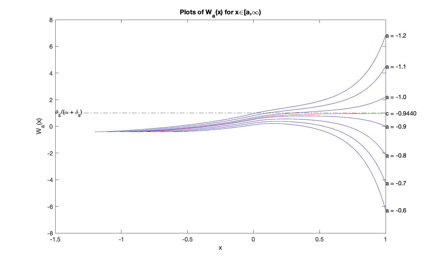
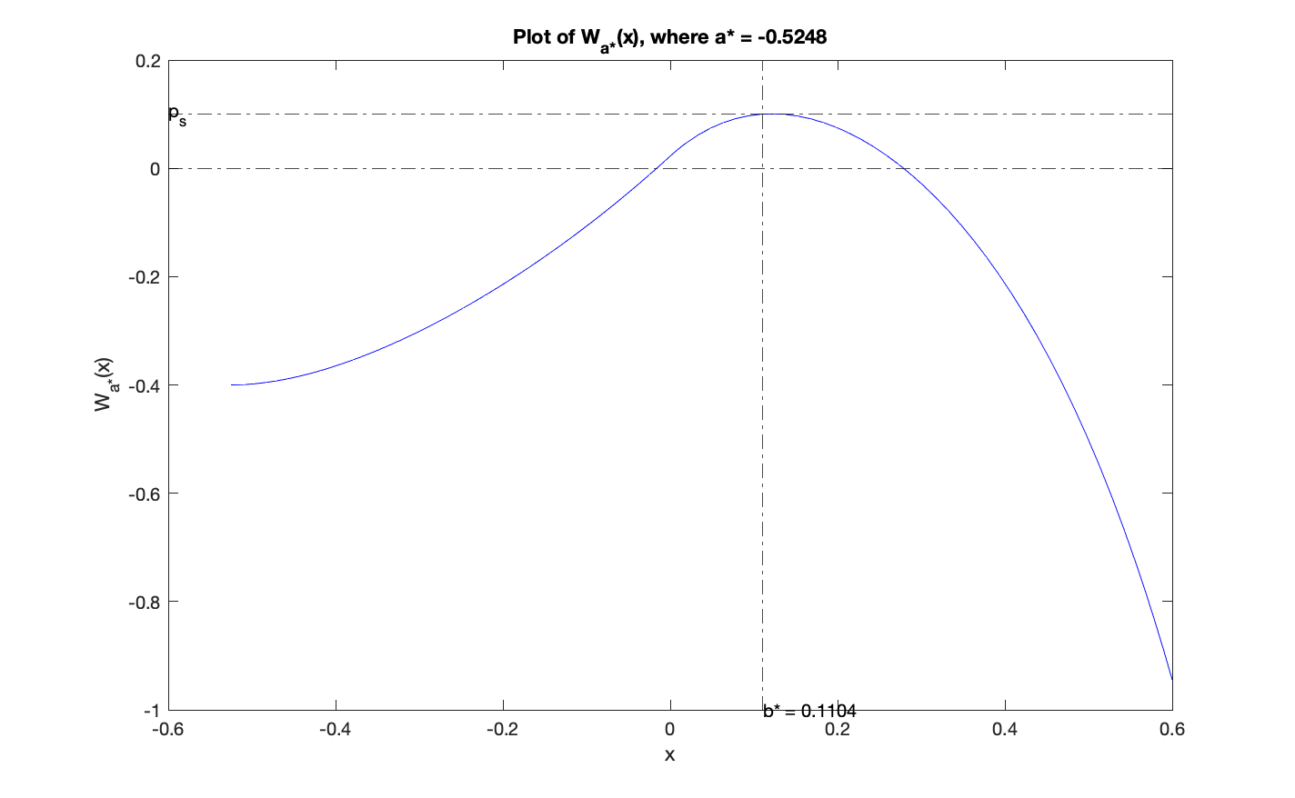
Example 4.1.
We set , and . It is easily seen that and We present two figures. In Figure 1, the plots of for are derived along with the value . One can observe that when , as , while when , as . In Figure 2, we find the values and .
Example 4.2.
We set and as in Example 4.1. We consider different values of and and observe the corresponding changes of the optimal buffer sizes. For convenience, we fix the value of , and let the value of vary. In this setting, the value of does not change. We summarize the numerical results in the following table. We observe that as approaches , both and increase and in particular, goes to .
| (buyer side) | (seller side) | |||||
5 Asymptotic Optimality
In this section, we establish the following two main results: In the first theorem (see Theorem 5.1), we prove the value function of the DCP given in (4.7) is an asymptotic lower bound for the sequence of value functions of the QCPs given in (2.14). In the second result, Theorem 5.3 exhibits an asymptotically optimal sequence of controlled queueing processes where the associated sequence of cost functionals converges to the value function Hence the lower bound described in Theorem 5.1 is achievable.
We simplify the form of the cost functional in (2.13) using Proposition 3.10 to match the form of the cost functional in (4.4). More precisely, from the proof of the following Theorem 5.1, the cost functional can be written in the following form
| (5.1) |
where We note that (5.1) is in agreement with the form of (4.4) for the DCP with a negligible term , and this plays an important role in establishing the asymptotic lower bound of the DCP for the QCP (Theorem 5.1).
Theorem 5.1 (Asymptotic lower bound).
Let be an admissible process for the system. Then
| (5.2) |
where is the value function of the DCP given in (4.7).
Proof.
We first show (5.1). In (2.13), using the Fubini’s theorem,
| (5.3) | ||||
Using (3.8) and (3.19), we have where the constant and the integer are independent of and Hence using (3.44) and Fubini’s theorem, we conclude that
| (5.4) |
By reversing the above procedure, we have
| (5.5) |
From (5.3) – (5.5), , and similarly, Recall the following parameters from the DCP (4.4), and , and the effective running cost function defined in (4.5). Hence, the cost functional can be written in the form of (5.1).
Now fix Let be an arbitrary admissible strategy in (4.6). We first establish for all , where is a constant independent of as well as the strategy Using the It’s formula to in (4.1) and the fact we obtain
| (5.6) |
where Notice that , where and Using this in the RHS of (5.6), we obtain for all .
Let be arbitrary and pick so that . We now consider Let be an admissible process which satisfies (3.53). By Theorem 3.1, we consider any limit point in which satisfies (3.4). Using (5.1), integration by parts, and the Fatou’s lemma, we obtain
Next, we extend on to the process on in by letting and for all and satisfies (3.4). Then is an admissible strategy for the DCP in (4.6) and satisfies where Hence for every and . Letting , then (5.2) follows and the proof is complete.
Our next aim is to construct an asymptotically optimal sequence of processes to achieve the lower bound in (5.2). There will be four different types of asymptotically optimal state process sequences corresponding to the four types of optimal controls for the DCP constructed in Theorem 4.2.
For each we consider a diffusion-scaled state process which satisfies (2.12) with time-independent reflection barriers at and initial data Here takes values in a lattice of the form and hence, the initial position as well as the reflecting barriers and are assumed to take values in the same lattice as well. We choose the sequences and in the lattice so that and where In the following lemma, for the simplicity of the presentation, we assume but if is outside the interval then there is an initial jump at time to the nearest point in from Since the jump size of this possible jump is and it is bounded, the conclusion of the lemma clearly holds for this general case.
Lemma 5.2.
Let and satisfy (2.12) with time-independent reflection barriers at and initial data We assume there is a so that for all , and for each the process and take values in the lattice . Then the following moment bound holds:
| (5.7) |
where the constant and the integer are independent of and
Proof.
We notice which satisfies (2.12) with reflection barriers at is the unique solution to the SP (see [23]) on with the input process as given in (3.2) and (3.6). To use the comparison theorem for the constraint processes, we consider for
where Let
where and Since both and are nondecreasing, using the comparison theorem (Theorem 1.7 of [23]) for and , we have
| (5.8) |
Next using the comparison theorem for and , we have
| (5.9) |
| (5.10) |
We note that the processes and are independent. Hence is a pure jump process with jump size Next, we rely on the oscillation inequalities (see Proposition 4.1 part (ii) (c) in [39] or [7]) to obtain an upper bound for For any in let be defined by (1.1), then using Proposition 4.1 part (c) of [39] we obtain for some independent of and so that
| (5.11) |
A similar estimate can be obtained for Next, using this estimate, (5.10), (3.9) and Proposition 3.8 (i), we can easily obtain (5.7). This completes the proof.
Theorem 5.3 (Asymptotic optimality).
Under Assumptions 2.1 – 2.5, the following results hold. Let and be as in Theorem 4.2.
-
(i)
When and , the sequence of processes with the zero control policy and for all is asymptotically optimal.
-
(ii)
When and , for satisfying and , the associated sequence of the two-sided reflected processes with reflecting boundaries at and provides an asymptotically optimal sequence.
-
(iii)
When and , for satisfying , the corresponding sequence of the one-sided reflected processes with reflecting boundary at yields an asymptotically optimal sequence.
-
(iv)
When and for satisfying , the corresponding sequence of the one-sided reflected processes with reflecting boundary at yields an asymptotically optimal sequence.
Proof.
Let be fixed. By Theorem 4.2 (i), zero control strategy is optimal for the DCP when and The corresponding state process is the unique strong solution to (4.12). Moreover, the value function of the DCP is given by
We now consider the process with the zero control policy and for all . Then by (3.53), where in probability for any Using Theorem 11.4.5 of [43], (3.3), the Lipschitz continuity of and following Theorem 2.11 of [38], we conclude that converges weakly to in Let be arbitrary. Using (3.8) and the Lipschitz continuity of , we can find a large so that
Since converges weakly to in using (3.8), we obtain
and therefore,
Since is arbitrary, Using (5.2), we obtain Hence part (i) follows.
To prove part (ii), consider satisfying (4.13) with reflection barriers at and It is an optimal control for the DCP in this parameter regime as proved in Theorem 4.2 (ii). Our aim is to construct an asymptotically optimal sequence which converges weakly to For each we consider a state process which satisfies (2.12) with time-independent reflection barriers at and initial data as described in Lemma 5.2. Here we choose and so that and
We assume (2.1) and consider the case Then the state equation can be written in the form (3.53) and converges weakly as in (3.3). Using the Skorokhod representation theorem, we assume that all these processes are defined in a same probability space and The reflected diffusion process is a strong solution to (4.13) in this probability space with respect to the same Brownian motion Next, we use Proposition A.7 in Appendix A to conclude and for any Next let be arbitrary. Using the moment bounds in (3.8) and (5.7), we can find a so that
and similarly,
Using the convergence of to almost surely on and by an argument similar to part (i), we can conclude that and consequently, This complets the proof of part (ii).
Proofs of parts (iii) and (iv) uses only the one-sided Skorokhod map and hence the proofs are much simpler than part (ii). In each case, the proof is very similar to that of Theorem 4.2 in [41]. Therefore, we omit it here.
Appendix A Two-sided Skorokhod maps
In this sub-section, we establish several results to supplement the work of [23, 34] and Chapter 14 of [43]. These results enable us to obtain asymptotically optimal strategies in Theorem 5.3. We first revisit the definition of the two-sided Skorokhod map (see Definition 1.2 in [23]). We follow the notation in [23], and let represent the two-sided Skorokhod map on the (time-independent) interval .
Definition A.1.
Let the constants . Given , there exists a unique pair of functions and of bounded variation such that
-
(i)
for each , ;
-
(ii)
, , and has the decomposition satisfying that and are non-decreasing, and
The map that takes to the corresponding is referred to as the two-sided Skorokhod map on , and the triple is referred to as the Skorokhod decomposition of on From the comparison properties of the Skorokhod map on (Theorem 1.7 of [23]), the Skorokhod decomposition is unique.
Lemma A.1.
Let Then for any in
| (A.1) |
Proof.
Using equation (1.14) in [23] and the notation therein, for any in ,
| (A.2) |
where for and , and for , We notice that
and
From (1.16) of [23], we have for any and in Hence
| (A.3) | ||||
In the next result, we consider two convergent sequences and so that is increasing to , and is decreasing to as Let be a convergent sequence in so that for each , where is a continuous function. We introduce
| (A.4) |
and
| (A.5) |
where is a Lipschitz continuous function.
Consider the Skorokhod decomposition of the function on the interval , and the Skorokhod decomposition of the function on Next, we obtain the convergence results of the Skorokhod decompositions of and This proof is closely related to that of Proposition 4.2 of [34].
Proposition A.2.
There exists a constant which depends only on and the Lipschitz constant of the function such that
| (A.6) |
Consequently, and
| (A.7) |
Proof.
The existence and uniqueness of solutions to (A.4) and (A.5) depend only on the Lipschitz continuity of the function as shown in Lemma 4.2 of [34]. Using the Lipschitz continuity of in (A.4) and (A.5), we obtain where is a constant depending on the Lipschitz constant of the function . Then,
| (A.8) | ||||
Now using (A.3) and the Lipschitz property of , for each we obtain,
| (A.9) |
Employing the Gronwall’s inequality leads to
| (A.10) |
and hence Next we note that Using (A.1) and the Lipschitz property of we obtain Consequently, using (A.10), (A.6) follows and thus the proof of part (i) is complete.
To prove part (ii), we let and for all . By part (i), Next we follow the proof of Theorem 14.8.1 in [43]. Let be arbitrarily small satisfying Let where Let where Inductively, let where and where Since is a continuous function, also continuous on Consequently, there are only finitely many points Let so that for any . For as well as increases only on a finite number of intervals of the form say On those intervals, and remain constant. Moreover, and remain constant on the intervals On each interval , only the one sided Skorokhod map (see equation (1.4) in [23]) will be applied. Hence, it is evident that on each interval. Consequently, follows. This completes the proof.
The following results are immediate from the above proposition.
Corollary A.1.
The Skorokhod decomposition converges to in in Skorokhod -topology.
Corollary A.2.
Let be in be fixed. Consider the Skorokhod decompositions and of on and , respectively. Assume that and Then
| (A.11) |
and
| (A.12) |
At last we consider the two-sided SP on time dependent intervals. The following definition is from [5].
Definition A.2.
Let , where could take and could take . Given so that for , a pair of functions is said to solve the SP for on the time-dependent interval if and only if it satisfies the following properties.
-
(i)
for each , ;
-
(ii)
has the decomposition , where and are non-decreasing functions, and
If there is a unique solution to the SP for on , then we write , where will be referred to as the two-sided Skorokhod map on , and the triple is referred to as the Skorokhod decomposition of on
From Theorem 2.5 and Corollary 2.4 of [5], if , then there is a unique pair that solves the SP for , and from the composition properties (Section 3 in [5]), the corresponding Skorokhod decomposition is unique.
Next we develop the oscillation inequalities for the constrained processes of Skorokhod decomposition. For a function in we recall its oscillation in an interval is defined by (1.1), and the modulus of continuity is given in (1.2).
Proposition A.3.
Let the functions and be in and for all Given a function in let be the unique solution to the SP in satisfying for all and be a function of bounded variation on as described in Theorem 2.6 of [5]. Then for all and ,
| (A.13) |
Proof.
Using Theorem 2.6 and Corollary 2.4 of [5], we can write for where
| (A.14) |
where
| (A.15) |
and
| (A.16) |
for all
Since it is evident that
| (A.17) |
From (A.14), it follows that
| (A.18) |
Next, we estimate and carefully. Using (A.15), we obtain whenever Therefore, . Similarly, for we can use (A.16) together with the simple inequality to obtain
| (A.19) |
Now combining (A.17) through (A.19), we obtain (A.13). This completes the proof.
Remark A.1.
Following the above proof, one can obtain the inequality
on any given interval
Proposition A.4.
Let in be the solution to the SP with the input function in and the time-dependent barriers and which are also in Assume and Then the following oscillation inequalities hold for any :
| (A.20) |
and
| (A.21) |
where is a generic constant independent of and and
Proof.
We focus on proving (A.20) the oscillation property for below and the proof of (A.21) is similar. The proof is divided into the following three steps.
Step 1. Oscillation inequality in where is a constant:
Using Theorem 4.2 of [7],
The constant is independent of the functions and as well as the domain
Since set of piecewise constant functions are dense in with respect to uniform norm (see [43], Theorem 12.2.2.), we assume is piecewise constant. Then also piecewise constant with the same points of discontinuity. We can use the construction of in the equation (8.2) of Chapter 14 of [43]. Let be the points of discontinuity of Then, holds at each jump point . Hence we obtain when is a piecewise constant function. This inequality can be generalized for any in using Proposition A.7 and (A.6) by taking the function to be identically zero. Hence follows.
Step 2. Oscillation inequality in where is in
We assume Consider the triple corresponding to the input function We pick in We pick so that For convenience assume is not a point of discontinuity of Now consider the interval If choose and If choose
Now is the solution to the SP for on and let be the solution to the SP for on Then by the comparison theorem in Proposition 3.5 of [6], (with identically zero), we have
Next we compare the solution of on the time dependent interval with the solution of on We use the comparison theorem in Proposition 3.3 of [5] to conclude Using Step 1, we obtain Consequently,
Hence holds in when is in and
Step 3. Oscillation inequality in with
We can use the proof of Lemma 2.2 and equation (2.26) in [36] to observe that the corresponding constraining processes are unchanged under translation by the function there. Let for all in Hence using Step 2, we obtain But Hence we have and this yields (A.20) and the proof is complete.
For a given by choosing intervals of length less than and using (A.20) and (A.21), we can obtain the following corollary.
Corollary A.3.
Let in be the solution to SP for in and the time-dependent barriers and in so that and Let be as in (1.2). Then
| (A.22) |
and
| (A.23) |
where is a generic constant independent of and
Appendix B Constructing the solutions of the HJB
B.1 Proof of Proposition 4.3
Our approach here is to find two bounded solutions in the domains and so that we can paste them smoothly at the origin. On (4.18) can be written as Since is a particular solution, has the representation where satisfies the homogeneous equation
| (B.1) |
Since we expect to be bounded, we seek for a bounded non-trivial solution for A fundamental set for this homogeneous equation consists of one bounded function and another unbounded function as tends to infinity. We need only to seek for this bounded solution. Such a solution exists and has a stochastic representation (see Section 50 of Chapter V in [35]): Consider a solution to the Ornstein-Uhlenbeck type equation where is a standard Brownian motion and consider the stopping time Then for is such a bounded solution to the homogeneous equation (B.1) and any other bounded solution in is a constant multiple of Moreover, and it is a strictly decreasing function on We expect to be of the form in the interval where is a constant which needs to be determined. Since it follows that
We can perform a similar analysis on the interval Notice that is a particular solution to (4.18) on Let where and is a standard Brownian motion. Introduce the stopping time and let for Then is a bounded solution to the homogeneous equation
Moreover, and it is strictly increasing in (for details, see Section 50 of Chapter V in [35]). Then similar to above analysis, we expect to be of the form when The constant needs to be determined. Then also follows.
Finally, to determine the constants and , we impose the “smooth fit conditions” for across the origin as they are described by and We use and Then, implies The condition implies By solving these equations and using the condition we obtain
Consequently, for this pair of and , the above described strictly increasing function on which satisfies (4.18). Moreover, is continuous everywhere except at It also satisfies (4.20) and (4.21) at the origin. Hence the proofs of parts(i), (ii) and (iii) are complete and it remains to show the uniqueness of
To prove the uniqueness, we consider where is a standard Brownian motion. The condition implies the explosion time of is infinite. Since and are finite, we can apply It’s lemma (see [17]) to to obtain the representation Hence the uniqueness of follows.
B.2 Proof of Proposition 4.4
Let the cost parameters and satisfy and Throughout, we use continuity properties of the solutions with respect to initial data and other parameters and we refer to Chapter V of [15]. First we gather a few useful facts about the differential equation (4.18). Recall that is a constant solution on the interval and on is a constant solution for (4.18).
Lemma B.1.
Let satisfy (4.18) in the neighborhood of a point and assume Then the following hold.
-
(i)
If and then and is a strict local minimum.
-
(ii)
If and then and is a strict local maximum.
Proof.
If and satisfies (4.18) together with then we observe that Then the conclusion of part (i) is straightforward. The proof of part (ii) is similar and is omitted.
Remark B.1.
Notice that if and then by the uniqueness of solutions to the differential equation (4.18), it follows that for all Similar conclusion holds when and
For each we let be the solution to (4.18) on with the initial data and Since is a particular solution to (4.18) on the interval we can express as follows:
| (B.2) |
where is a solution to the homogeneous equation given below:
| (B.3) |
with the boundary conditions
| (B.4) |
For the homogeneous differential equation (B.3), there exists a fundamental set of solutions on satisfying These solutions and have stochastic representations as described in Chapter V of [35] (see Section 50 and in particular Proposition 50.3.). Moreover, is strictly increasing and is strictly decreasing in the domain
Lemma B.2.
Let then the following hold for each solution
-
(i)
Each is strictly decreasing on and strictly increasing on Moreover, and are finite.
-
(ii)
and .
Proof.
By (B.2), it suffices to prove the lemma for To show part (i), we observe that for any if and for some then by (B.3), and is necessarily a strict local minimum. In particular, for and by (B.4), is a strict local minimum. With the absence of any local maxima when we observe that is strictly decreasing in and strictly increasing in Moreover, the coefficients of the differential equation (B.3) can be linearly and continuously extended to Hence and are finite. This proves part (i).
For part (ii) let Using the fundamental set we can write for all , where and are constants. Since has a positive, strict local minimum at t is strictly decreasing in and strictly increasing in for some Since is strictly increasing and is strictly decreasing, it follows that and But is a bounded function on and Hence, and consequently, holds.
To show let By (B.4), and meet at a point in the interval and But by the uniqueness of solutions, two solutions to a homogeneous equation cannot meet more than once. Therefore, Consequently, is finite or else it is Suppose is finite. Then for all Moreover, and for each By integrating (B.3) and using and is a non negative increasing function in , we obtain the bound Since is bounded, RHS of this inequality tends to , when tends to But is bounded above by the constant which is finite. This yields a contradiction. Hence, and this completes the proof.
From the above discussion, satisfies the linear equation (4.18) on and and are finite. For each we can extend to so that it satisfies (4.18) on with the available initial data for and More precisely, on the interval satisfies
| (B.5) |
We let
| (B.6) |
Then satisfies the homogeneous equation
| (B.7) |
together with the boundary data and Similar to on , there is a fundamental set of solutions for the above homogeneous equation on so that , , is strictly decreasing and is strictly increasing on (See Chapter V of [35] for a stochastic representation of and ) Hence each can be written as
| (B.8) |
where and are constants.
In the next two results, we show that when there are two types of solution profiles of which exhibits very different behavior on When is very large, tends to as When is small, tends to as These two profiles are separated by the solution curve of , where is a special point. The solution is bounded on and it approaches as
Lemma B.3.
There exists a so that if then
-
(i)
has a local maximum in ;
-
(ii)
Proof.
We first consider which corresponds to . Then satisfies (4.18) everywhere except at and Moreover, and are continuous everywhere, has a jump discontinuity at and Following the proof of Lemma B.1 (i), is strictly decreasing on On , since and by a similar argument, is strictly decreasing.
We can then choose and so that Note that both and satisfy (4.18) on Hence, using the continuity of the solutions in initial data, for any there exists a so that whenever The functions and satisfy (B.5) in Again using the same continuity property, we can find a so that whenever Now, by letting we can find a so that whenever Hence, each is strictly increasing in , and . Thus, has a local maximum in This completes part (i).
From part (i), has a local maximum at a point in Thus,
which yields that But cannot be equal to ; otherwise becomes the unique solution as explained in Remark B.1, which contradicts with the fact that is strictly decreasing on . Hence and for Using (B.5), then it follows that is strictly concave and strictly decreasing for large Hence, part (ii) follows.
Next we consider the properties of the solution when and is very large. From Lemma B.2 (ii), we can find a constant so that
| (B.9) |
Lemma B.4.
Let where is given in (B.9). Then
-
(i)
is strictly increasing on the interval ;
-
(ii)
Proof.
By Lemma B.2 (i), (equivalently, ). The differential equation (B.3) can be continuously and linearly extended to Hence we consider the corresponding extended solution as given in (B.2) and (B.6). Next, we show that Suppose Then by (B.9) and (B.7), we have Thus has a strict local minimum at the origin. This is a contradiction since is strictly increasing in Hence and consequently, Thus, we can find a so that when Let Suppose is finite. Then and Hence, and is a strict local minimum. This is a contradiction since in Hence and part (i) follows.
By part (i) and (B.6), is strictly increasing on Then exists and suppose it is finite. Then, and in (B.8). Thus, and by (B.6), It contradicts with (B.9) since is increasing on . Hence, and by (B.6), part (ii) follows.
Lemma B.5.
There exists a point so that
-
(i)
the solution is strictly increasing in ;
-
(ii)
is bounded in and
Proof.
Let . By Lemmas B.3 and B.4, such a point exists and Moreover, is strictly increasing on and thus Suppose then from (B.5) and by the fact that This is a contradiction since is strictly increasing in Hence and there is a so that over We let Clearly, Suppose that is finite. Then If using (B.5), This is a contradiction since is strictly increasing in Thus Now if by the uniqueness of solutions, is a constant on and this contradicts with Hence the only possibility is in which case and is a strict local maximum and is strictly decreasing on Similar to the proof of Lemma B.3 (ii), we see that Now using the continuity of the solutions with respect to the parameter , we can find a so that for each This contradicts with the definition of Hence is infinite and part (i) follows.
From part (i), exists. Suppose We can pick so that Using the continuity of and with respect to , we can find a so that for each and on By the proof in Lemma B.4, each such increases to and this contradicts with the definition of . Hence and is bounded in and equivalently, defined in (B.6) is also bounded. By (B.8), we can write for Since is bounded, we have and thus, for But and consequently Using this together with (B.6), we obtain This completes the proof.
In the next lemma, we establish the uniqueness of the point
Lemma B.6.
For , let be the corresponding solution of (4.18) so that is finite. Then and for all
Proof.
Suppose and satisfies the assertion. Without loss of generality, let We note that and from Lemma B.2, and are strictly decreasing on and respectively, and are strictly increasing on and respectively. Hence and meet at a point where , and moreover, Next, following the argument of Lemma B.5 (ii), we conclude that
We now consider for Then and Moreover, is a bounded solution to the homogeneous equation We let so that Then and When using the differential equation for at , we obtain and thus, is a local minimum, which contradicts with the definition of . Hence Again, by the differential equation, we obtain and thus is strictly decreasing in for some which is again a contradiction because is the maximum. Hence and the conclusion of the lemma follows.
Let be as in Lemma B.5.
Lemma B.7.
For for all has a unique local maximum on and thereafter it is decreasing to , i.e., Moreover, if then for all
Proof.
Similar to the argument in the proof of Lemma B.6, and meet at a point , and . Suppose that and meet at a point We consider for , and define . Following an argument similar to the proof of Lemma B.6, we can obtain a contradiction on , and thus for all Consequently, for all . By Lemma B.1, can have at most one local maximum and no local minima. If has no local maxima, then it is increasing and bounded above by , and is finite. Using Lemma B.6, we have and this is a contradiction. Therefore, each has exactly one local maximum in and thereafter is decreasing. Again using Lemma B.6, we must have The proof of the last assertion is very similar to the above proof of for all And it is omitted. This completes the proof.
For , assume that each achieves the unique local maximum at We introduce the function by
| (B.10) |
Proposition B.8.
The following results hold for the function defined in (B.10).
-
(i)
The function is a continuous strictly decreasing function.
-
(ii)
and and is an on-to function.
-
(iii)
Given there is a unique in so that Let Then the corresponding is strictly increasing in and and the triple satisfies all the conditions in Proposition 4.4.
Proof.
The strictly decreasing property of the function follows from Lemma B.7. To show the continuity of we fix so that . Since the solution to (4.18) is continuous with respect to the initial data, for a given there exists a so that implies Let , and choose so that Next, satisfies (B.5) on and the coefficients of this differential equation can be smoothly extended to Using the continuity property of initial data for this extended linear equation, for any , we can find so that guarantees Now choose . Then implies By Lemma B.7, implies for all and . Consequently, when , from Lemma B.7, Thus, Similarly, when it follows that This proves the continuity of at The proof of part (i) is complete.
Since is strictly decreasing and is an upper bound, exists and it is less than or equal to Again by the continuity property of the initial data, is close to when is very close to Using this together with Lemma B.5 (ii), it follows that The proof of is similar. These limits together with part (i) implies that is an onto function.
Finally, part (iii) is a consequence of parts (i) and (ii). This completes the proof.
Remark B.2.
Acknowledgements: Ananda Weerasinghe is partially supported by the Simons Foundation grant 317381 and grateful for their support.
References
- [1] Akan, M., Alagoz, O., Ata, B., Erenay, F.S. and Said, A., A broader view of designing the liver allocation system, Operations research, 60 (2012), pp.757-770.
- [2] Atar, R., Mandelbaum, A. and Reiman, M. I., Scheduling a multi-class queue with many exponential servers:Asymptotic optimality in heavy traffic , Ann. Appl. Probab., 14 (2004), pp. 1084-1134.
- [3] Billingsley, P., Convergence of Probability Measures, second edition, John Wiley and sons, New York (1999).
- [4] Boxma, O. J., Israel, D., Perry, D. and Stadje, W., A new look at organ transplantation models and double matching queues, Probability in the engineering and information sciences 25 (2011), pp 135–155.
- [5] Burdzy, K., Kang, W. and Ramanan, K., The Skorokhod problem in a time-dependent interval, Stoch. Proc. and their Appl., 119 (2009), pp. 428-452.
- [6] Conolly, B. W., Parthasarathy, P. R., and Selvaraju, N.,, Double-ended queues with impatience, Computers & Oper. Res., 29 (2002), pp. 2053–2072.
- [7] Dai, J. G. and Dai, W., A heavy traffic limit theorem for a class of open queueing networks with finite buffers, Queueing Syst., 32 (1999), pp. 5–40.
- [8] Dai, J. G. and He, S., Customer abandonment in many-server queues, Math. Oper. Res., 35 (2010), pp. 347-362.
- [9] Ethier, S. N. and Kurtz, T. G., Markov Processes: Characterization and Convergence, Wiley, New York (1986).
- [10] Fleming, W. H. and Soner, H. M., Controlled Markov Processes and Viscosity Solutions, Second edition, Springer-Verlag, New York (2006).
- [11] Gurvich, I., and Ward, A., On the dynamic control of matching queues, Stoch. Syst., 4 (2014), pp. 479–523.
- [12] Halfin, S. and Whitt, W., Heavy traffic limits for queues with many exponential servers, Oper. Res. 29 (1981), pp. 567-588.
- [13] Harrison, J. M., Assembly-like queues, Journal of Appl. Probab. 10 (1973), pp. 354-367.
- [14] Harrison, J. M., Brownian Motion and Stochastic Flow Systems, Wiley Publications, New York (1985).
- [15] Hartman, P., Ordinary Differential Equations, Wiley Publications, New York (1964).
- [16] Jacod, J., and Shiryaev, A. Limit theorems for stochastic processes. Springer Science & Business Media (2003).
- [17] Karatzas, I. and Shreve, S.E., Brownian Motion and Stochastic Calculus, Springer-Verlag, New York (1988).
- [18] Kashyap, B. R. K., The double-ended queue with bulk service and limited waiting space, Oper. Res. 14 (1966), pp. 822-834.
- [19] Kaspi, H. and Perry, D., Inventory systems of perishable commodities, Adv. Appl. Prob. 15 (1983), pp. 674–685.
- [20] Khademi, A. and Liu, X., Asymptotically optimal allocation policies for transplant queueing systems, Working Paper (2020).
- [21] Kocaga, Y. L. and Ward, A., Admission control for a multi-server queue with abandonment, Queueing Systems, 65 (2010), pp. 275-323.
- [22] Krichagina, E. V. and Taksar, M., Diffusion approximation for GI/G/1 controlled queues, Queueing Systems Theory Appl., 12 (1992), pp. 333-367.
- [23] Kruk, L., Lehoczky, J., Ramanan,K. and Shreve, S., An explicit formula for the Skorokhod map on [0,a], Ann. Appl. Probab., (2007), pp. 669-682.
- [24] Lee, C., Liu, X., Liu, Y. and Zhang, L., Optimal control of a time-varying double-ended production queueing model, working paper (2020).
- [25] Liu, X., Diffusion approximations for double-ended queues with reneging in heavy traffic, Queueing Syst., (2018), pp. 1–39
- [26] Liu, X., Gong, Q., and Kulkarni, V. G., Diffusion models for double-ended queues with renewal arrival processes, Stoch. Syst., 5 (2015), pp. 1–61.
- [27] Meyer, P. A., Un cours sur les integrales stochastiques, Seminaire de Probabilities X, Lecture Notes in Math. 511, Springer, New York (1974).
- [28] Pang, G., Talreja, R. and Whitt, W., Martingale proofs of many-server heavy-traffic limits for Markovian queues, Probability Surveys, 4 (2007), pp. 193-267.
- [29] Perry, D. and Stadje, W., Perishable inventory systems with impatient demands, Math. Methods of Oper. Res., 50 (1999), pp. 77–90.
- [30] Plumbeck, E. L., and Ward, A. R., Optimal control of a high-volume assemble-to-order system, Math. Oper. Res., 31 (2006), pp. 453–477.
- [31] Prabhakar, B., Bambos, N., and Mountford, T. S.,, The synchronization of Poisson processes and queueing networks with service and synchronization nodes, Adv. Appl. Probab., 32 (2000), pp. 824–843.
- [32] Protter, P., Stochastic Differential Equations, Second edition, Springer-Verlag (2004).
- [33] Reed, J. E., The queue in the Halfin-Whitt regime, Ann. Appl. Probab. 19 (2009), pp. 2211–2269.
- [34] Reed, J. E. and Ward, A. R., Approximating the queue with a nonlinear drift diffusion: hazard rate scaling in heavy traffic, Math. Oper. Res., 33 (2008), pp. 606–644.
- [35] Rogers, L. C. G. and Williams, D., Diffusions, Markov Processes and Martingales, Volume 2, Cambridge University Press, (2000).
- [36] Slaby, M, Explicit representation of the Skorokhod map with time dependent boundaries, Probability and Mathematical Statistics 30 (2010): pp. 29-60.
- [37] Song, J. S., and Zipkin, P., Supply chain operations: Assemble-to-order and configure-to-order systems, Handbook in Oper. Res. and Mgmt. Sci., Vol. XXX (2003), pp. 561–593.
- [38] Talreja, R. and Whitt, W., Heavy-traffic limits for waiting times in many-server queues with abandonment, Ann. Appl. Probab. 19 (2009), pp. 2137–2175.
- [39] Ward, A. R. and Kumar, S., Asymptotically Optimal Admission Control of a Queue with Impatient Customers, Math. Oper. Res., 33 (2008), pp. 167–202.
- [40] Weerasinghe, A., A bounded variation control problem for diffusion processes, SIAM J. Control and Opt., 44 (2005), pp. 389-417.
- [41] Weerasinghe, A. and Mandelbaum, A., Abandonment versus blocking in many server queues:asymptotic optimality in the QED regime, Queueing Syst., 75 (2013), pp. 279–337.
- [42] Weerasinghe, A., Diffusion approximations for queues with state dependent service rates, Math. Oper. Res., 39 (2014), pp. 207–228.
- [43] Whitt, W., Stochastic-Process limits, Springer Series in Operations Research, Springer-Verlag, New York. (2002).
- [44] Whitt, W., Proof of the martingale FCLT, Probability Surveys, 4 (2007), pp 268–302.
| Xin Liu | Ananda P. Weerasinghe | |
| O-324 Martin Hall | 396 Carver Hall | |
| School of Mathematical and Statistical Sciences | Department of Mathematics | |
| Clemson University | Iowa State University | |
| Clemson, SC 29634, USA | Ames, IA 50011, USA. | |
| xliu9@clemson.edu | ananda@iastate.edu |