Non-Gaussian Normal Diffusion in Low Dimensional Systems

Abstract

Brownian particles suspended in disordered crowded environments often exhibit non-Gaussian normal diffusion (NGND), whereby their displacements grow with mean square proportional to the observation time and non-Gaussian statistics. Their distributions appear to decay almost exponentially according to “universal” laws largely insensitive to the observation time. This effect is generically attributed to slow environmental fluctuations, which perturb the local configuration of the suspension medium. To investigate the microscopic mechanisms responsible for the NGND phenomenon, we study Brownian diffusion in low dimensional systems, like the free diffusion of ellipsoidal and active particles, the diffusion of colloidal particles in fluctuating corrugated channels and Brownian motion in arrays of planar convective rolls. NGND appears to be a transient effect related to the time modulation of the instantaneous particle’s diffusivity, which can occur even under equilibrium conditions. Consequently, we propose to generalize the definition of NGND to include transient displacement distributions which vary continuously with the observation time. To this purpose, we provide a heuristic one-parameter function, which fits all time-dependent transient displacement distributions corresponding to the same diffusion constant. Moreover, we reveal the existence of low dimensional systems where the NGND distributions are not leptokurtic (fat exponential tails), as often reported in the literature, but platykurtic (thin sub-Gaussian tails), i.e., with negative excess kurtosis. The actual nature of the NGND transients is related to the specific microscopic dynamics of the diffusing particle.

I Introduction

Possibly misinterpreting the original works of Albert Einstein and Marian Smoluchowski on Brownian motion, one tends to associate the normal diffusion of an ideal Brownian particle with the Gaussian distribution of its spatial displacements. Recent observations Granick1 ; Granick2 ; Bhatta ; Sung1 ; Sung2 ; Granick3 of Brownian motion in fluctuating crowded environments led to question the generality of this notion. Indeed, it implicitly assumes Fick’s diffusion Gardiner , whereby the directed displacements of an overdamped particle, say, in the $x$ direction, $\Delta x(t)=x(t)-x(0)$, would grow according to the asymptotic Einstein law, $\langle\Delta x^{2}(t)\rangle=2Dt$, and with Gaussian statistics. The probability density function (pdf) of the rescaled observable, $\delta_{t}=\Delta x/\sqrt{t}$, would thus be a stationary Gaussian function with half-variance $D$.

However, there are no fundamental reasons why the diffusion of a physical Brownian tracer should be of the Fickian type. For instance, in real biophysical systems, displacement pdf’s have been reported, which retain prominent exponential tails over extended intervals of the observation time, even after the tracer has attained the asymptotic condition of normal diffusion. Such an effect, often termed non-Gaussian normal diffusion (NGND), disappears only for exceedingly long observation times (possibly inaccessible to real experiments Granick1 ), when the displacement distributions eventually turn Gaussian, as dictated by the central limit theorem, without changes of the diffusion constant. Persistent diffusive transients of this type have been detected in diverse experimental setups Granick1 ; Granick2 ; Bhatta ; other1 ; other3 ; other4 . Extensive numerical simulations confirmed the occurrence of NGND in crowded environments featuring slowly diffusing or changing microscopic constituents (filaments Granick1 ; Bhatta , large hard spheres Sung1 ; Sung2 ; Granick3 , clusters Kegel ; Kob , and other heterogeneities Tong ; Cherstvy ).

The current interpretation of this phenomenon postulates the existence of one or more fluctuating processes affecting composition and geometry of the particle’s suspension medium Granick1 . It seems reasonable that, for observation times comparable with the relevant environmental relaxation time(s), the tracer displacements may obey a non-Gaussian statistics. The rescaled pdf’s, $p(\delta_{t})$, are expected to be Gaussian for both much shorter and much larger observation times, but with different half-variance: the free diffusion constant, $D_{0}$, for $t\to 0$ (no crowding effect) and the asymptotic diffusion constant, $D$, introduced above, for $t\to\infty$ (central limit theorem). The mechanism how the tracer’s normal diffusion sets in and the constant $D$ remains unaltered through the entire non-Gaussian transient, varies, instead, from case to case. In summary, key features of the NGND phenomenon appear to be: (i) its transient nature, whereby the observables taken into account are intrinsically non-stationary; (ii) a time-modulated instantaneous diffusivity of the tracer. As discussed in the following, these conditions can occur even in the absence of external (non-equilibrium) perturbations of the Brownian dynamics.

A simple heuristic explanation Granick1 of the NGND phenomenon models the effects of the slowly fluctuating environment in terms of an ad hoc distribution of the tracer’s diffusion constant. Imposing an exponential distribution of the diffusion constant with average $D$, a straightforward superstatistical procedure yields the exponential (Laplace) rescaled distribution, $p(\delta_{t})=\exp(-\delta_{t}/\alpha)/2\alpha$, with $\alpha^{2}=D$. A more suggestive NGND paradigm is provided by the notion of diffusing diffusivity Slater , whereby the asymptotic particle’s diffusion constant is replaced by a time fluctuating auxiliary observable, $D(t)$. Regarding $D(t)$ as a continuous stochastic process with average $D$ and time constant $\tau$, the distribution $p(\delta_{t})$ changes from exponential for $t\ll\tau$ to Gaussian for $t\gg\tau$; in both time regimes, the displacement diffusion is normal, with $\langle\Delta x^{2}(t)\rangle=2Dt$ Slater . Refined variations of these paradigms Metzler2 ; Jain1 ; Jain2 ; Tyagi ; Luo ; Sokolov ; Metzler , predict different exponential decays of the transient distributions. These phenomenological approaches have two major limitations, namely: (i) They fail to incorporate the free Gaussian diffusion detected in most real and numerical experiments at very short observation times, $t\to 0$, when crowding plays no role. This is because these approaches purportedly ignore the microscopic details of the actual diffusion mechanisms; (ii) They generally aim at “universal” non-Gaussian transient pdf’s, namely, at functions $p(\delta_{t})$ insensitive to $t$ over extended domains, $t<\tau$. [In the superstatistical models $\tau=\infty$.] However, even if this strategy may appear to agree with NGND observations for complex systems Granick1 ; Granick2 ; Bhatta ; Sung1 ; Sung2 ; Granick3 , it is obvious that to reproduce the exponential-Gaussian crossover, the transient rescaled distributions must assume the form $p(\delta_{t},t)$, i.e., they must depend explicitly on $t$.

This study focuses on the microscopic mechanisms responsible for NGND. To this purpose, motivated by a preliminary study PRR , we investigated, both numerically and analytically, directed diffusion of different idealized tracers in confined geometries. We selected low dimensional systems mostly inspired to cell biology RMP_BM ; Lipowski . For appropriately short observation times, NGND emerges as a transient effect of the time modulation of the tracers’ microscopic diffusivity. This effect can occur even in the absence of environmental fluctuations. It suffices to require that the tracer’s dynamics be governed by two concurring diffusion mechanisms, at least one of them characterized by a finite relaxation time, $\tau$. During transients times of the order of $\tau$, the displacement distributions can deviate from their asymptotic Gaussian profile also after normal diffusion has set in. Moreover, such deviations do not necessarily imply the emergence of “fatter” exponential tails (leptokurtic transients), but under certain conditions, the distribution tails can get “thinner” (platykurtic transients).

This observation suggests typical NGND features are to be found in much wider a class of diffusion systems. Indeed, contrary to experimental and numerical observations on extended systems, the NGND transient displacement distributions in low dimensional models, are found to depend on the observation time. This led us to address the question of phenomenological fitting functions capable of reproducing the $t$-dependence of the rescaled pdf’s, $p(\delta_{t},t)$. We also noticed that the $t$ dependence of the transient rescaled pdf’s can be suppressed, though not completely, by considering models where the onset of normal diffusion is controlled by some intrinsic time constant, which can be taken much shorter than the upper bound, $\tau$, of the non-Gaussian transient. This provides us with a criterion to formulate low dimensional models that better capture the known NGND phenomenology in complex systems.

The present paper is organized as follows. In Sec. II we elaborate on a toy discrete model of NGND proposed first in Ref. Slater and then revisited in Ref. PRR . The purpose of this section is to single out key NGND aspects, like the time scales regulating the diffusion mechanisms and the nature of the non-Gaussian transients, that is, lepto- versus platykurtic. In Sec. III we consider the diffusion of a two dimensional (2D) ellipsoidal Brownian particle in a highly viscous, homogeneous and isotropic fluid in thermal equilibrium. For observation times shorter than its rotational relaxation time, the particle does undergo normal diffusion. However, its instantaneous diffusivity in a given direction is modulated in time due to its elongated shape. This results in exponentially decaying transient distributions of the particle’s directional displacements. In Sec. IV we analyze the diffusion of a 2D self-propelling symmetric particle in a homogeneous and isotropic active medium with finite orientational relaxation time. NGND is characterized here by thin tails of the transient displacement distributions. In both cases, however, transients are governed by one time scale, only, their orientational diffusion time, $\tau$: on increasing the observation time, normal diffusion just anticipates the onset of the Gaussian statistics of the particle’s displacements. In Sec. V we introduce a phenomenological fitting function, $p_{\beta}(\delta_{t})$ for the rescaled displacement distributions, with only one adjustable parameter, $\beta$. This function is designed ad hoc to ensure normal diffusion with the observed diffusion constant, $D$, at any time, while $\beta$ encodes the $t$-dependence of the rescaled displacement distributions. Relevant values of the fitting parameter $\beta$ are $\beta=2$ for a Gaussian pdf, $\beta=1$ for a Laplace (exponential) pdf, $\beta<2$ for a leptokurtic pdf, and $\beta>2$ for a platykurtic pdf. In Sec. VI we analyze the NGND phenomenon in a narrow corrugated channel chemphyschem ; PNAS with fluctuating pores PRR . NGND occurs for time-correlated pore fluctuations, random and periodic, alike, and, more importantly, for observation times comprised between two distinct, controllable time scales. The correlation time of the pore fluctuations sets the transient time scale, $\tau$, whereas the average pore-crossing time governs the onset of normal diffusion. Upon choosing the former much larger than the latter, the NGND transient is made grow wider and the $t$-dependence of $\beta$ weaker. As a practical application of the tools introduced thus far, in Sec. VII we investigate the diffusion of a passive Brownian tracer in a periodic array of planar counter-rotating convection rolls. The peculiarity of this model is that, by tuning its dynamical parameters, transients can change from lepto- to platykurtic. Two are the systems’s characteristic time scales: the mean time for the particle to first exit a convection roll and its average revolution period inside the roll. At low (high) temperatures, the former (latter) time scale is larger and thus plays the role of transient time, $\tau$; accordingly, the NGND transients are leptokurtic (platykurtic). Finally, in Sec. VIII we summarize the main conclusions of our approach to NGND.

II A Discrete NGND Model

Though sounding exotic to some readers, the phenomenon of NGND turns out to be way more general than the more familiar Fickian diffusion. To make this point, we elaborate now on a coarse grained model, first proposed in Ref. Slater , which serves well the purpose of illustrating NGND in continuous systems of any dimensionality.

Let us coarse grain the trajectory of a tagged particle in the $x$ direction as the sum of small random steps, $\Delta x_{i}$, taken at fixed discrete times, $t_{i}=i\Delta t$, where $i=1,\dots N$ and $\Delta t=1$, for simplicity. Accordingly, the position of the particle at time $N$ is $x_{N}=\sum_{i=1}^{N}\Delta x_{i}$. A stochastic average over the particle’s steps $\Delta x_{i}$ yields the mean square displacement at time $N$,

$$\langle x_{N}^{2}\rangle=\sum_{i=1}^{N}\langle\Delta x_{i}^{2}\rangle+2\sum_{i\neq j}{}^{\prime}\langle\Delta x_{i}\Delta x_{j}\rangle,$$ (1)

where $\sum_{i\neq j}^{\prime}$ stays for $\sum_{i=1}^{N-1}\sum_{j=i+1}^{N}$. Sufficient conditions to establish normal diffusion are that: (1) the step directions are uncorrelated, $\langle\Delta x_{i}\Delta x_{j}\rangle=0$, that is, for any given $\Delta x_{i}$, displacements $\Delta x_{j}$ and $-\Delta x_{j}$, are equiprobable; (2) the variance, $\langle\Delta x_{i}^{2}\rangle$, of the step probabilities, $p(\Delta x_{i})$, are of the same order of magnitude, though not necessarily identical. These requirements are less stringent than the assumptions implicit in the standard random walker model for Brownian motion Gardiner .

Indeed, for the sake of generality, one should not rule out finite correlations of the step lengths Slater . For instance, we can assume that during each unit time step the particle’s diffusion is normal with time-dependent constant, $D_{i}$, i.e.,

$$p(\Delta x_{i})=(4\pi D_{i})^{-1/2}\exp(-\Delta x_{i}^{2}/4D_{i}).$$ (2)

This assumption guarantees that the directions of the particle’s steps are uncorrelated, while their length correlation is controlled by the auto-correlation of the time sequence of the constants $D_{i}$, which, in turn, is specific to the system at hand. It follows immediately that

$$\langle x_{N}^{2}\rangle=2\langle D\rangle N,$$ (3)

and

$$\langle x_{N}^{4}\rangle-3\langle x_{N}^{2}\rangle^{2}=12\mu_{D}\langle D\rangle^{2}N+24{\sum_{i\neq j}}^{\prime}C_{ij},$$ (4)

with $\mu_{D}=(\langle D^{2}\rangle-\langle D\rangle^{2})/\langle D\rangle^{2}$ and $C_{ij}=\langle D_{i}D_{j}\rangle-\langle D_{i}\rangle\langle D_{j}\rangle$. For any given stationary model, there exists an appropriate distribution of the constants $D_{i}$, $p(D_{i})$, so that $\langle D_{i}\rangle\equiv\langle D\rangle$.

Suppose now that two particle steps, $\Delta x_{i}$ and $\Delta x_{j}$ are statistically uncorrelated only for large time differences, i.e., $\langle D_{i}D_{j}\rangle=\langle D_{i}\rangle\langle D_{j}\rangle$ for $|i-j|>\tau$. We then distinguish two limiting cases,

(i) $N\gg\tau$, where

$$\mu_{x}=\frac{\langle x_{N}^{4}\rangle-3\langle x_{N}^{2}\rangle^{2}}{\langle x_{N}^{2}\rangle^{2}}=\frac{3\mu_{D}}{N}\rightarrow 0.$$ (5)

A vanishing excess kurtosis, $\mu_{x}$, hints at a Gaussian $x_{N}$ distribution. This is the asymptotic limit of the displacement distributions predicted by the central limit theorem.

(ii) $N<\tau$, where

$$\mu_{x}=\frac{\langle x_{N}^{4}\rangle-3\langle x_{N}^{2}\rangle^{2}}{\langle x_{N}^{2}\rangle^{2}}=3\bar{\mu}_{D}.$$ (6)

with $\bar{\mu}_{D}=(2/N^{2}\langle D^{2}\rangle)\sum_{i\neq j}{}^{\prime}C_{ij}$. Eqs. (3) and (6) embody the definition of NGND. The finite excess kurtosis, $\mu_{x}$ depends on the actual auto-correlation of the constants $D_{i}$. For instance, on assuming $\langle D_{i}D_{j}\rangle=\langle D^{2}\rangle$ for all $i$ and $j$ with $|i-j|<\tau$, we obtain $\bar{\mu}_{D}=\mu_{D}$. In particular, for the exponential distribution $p(D_{i})=\exp(-D_{i}/\langle D\rangle)/\langle D\rangle$ assumed in the diffusing diffusivity model of Ref. Slater , $\mu_{D}=1$. Not surprisingly, the resulting value of the excess kurtosis, $\mu_{x}=3$, corresponds to a Laplace distribution of the total displacement $x_{N}$ Slater .

Of course a more realistic choice of the correlator $C_{ij}$ can yield different values of $\mu_{x}$. In most applications $C_{ij}$ is definite positive and decays to zero with time, i.e., with $|i-j|$; hence $0<\mu_{x}<3$, Accordingly, the corresponding $x_{N}$ distributions are leptokurtic, with tails decaying slower than those of a Gaussian distribution, but typically faster than exponentially. On the other hand, we cannot exclude the possibility that $C_{ij}$ decays to zero oscillating. This implies that, in principle, $\mu_{D}$ can assume negative values, so that the corresponding transient distribution of $x_{N}$ may be platykurtic. In Refs. nonG1 ; nonG2 ; nonG3 the present approach has been extended also to microscopically non-Gaussian diffusive processes [where the $\Delta x$ distribution of Eq.(2) does not apply].

We conclude this section with a final remark about the time scales involved in this discrete model. One time scale has been introduced explicitly, namely the characteristic decay time, $\tau$, of the correlator $C_{ij}$ or, equivalently, the correlation time of the step lengths, $\Delta x_{i}$. A second one is implicit in our choice for the step distribution, $p(\Delta x_{i})$. In Eq. (2) the coarse grained diffusion was assumed to be normal over the time step $\Delta t=1$. This implies that in the corresponding continuum system normal diffusion is expected to have occurred at some intrinsic time scale much shorter than $\tau$. Of course the discrete model of this section cannot reproduce the diffusion properties at times shorter than the discretization time scale, $\Delta t$.

III Diffusion of an Ellipsoidal Particle

We consider first the simple case of a 2D ellipsoidal particle of semiaxes $a$ and $b$, with $a>b$, diffusing in a highly viscous, homogeneous and isotropic medium, subject to equilibrium thermal fluctuations. This is a well-known problem in biological physics Berg . The particle’s elongation causes a dissipative coupling between the center of mass translational degrees of freedom, $x$ and $y$ in the laboratory frame, and the rotational degree of freedom, $\theta$. As sketched in Fig. 1(b), the angle $\theta$ defines the orientation of the particle’s long axis with respect to the horizontal $x$ axis. The physical consequences of such a mechanism were first recognized by F. Perrin Perrin . An ellipsoidal particle tends to diffuse independently in directions parallel and perpendicular to its long axis, that is along its principal axes. The relevant diffusion constants in the body frame are denoted here by $D_{a}$ and $D_{b}$, with $D_{a}\geq D_{b}$. In 2D, rotational diffusion is governed by an additional diffusion constant, $D_{\theta}$, which will be handled here as unrelated to the translational constants, $D_{a}$ and $D_{b}$, to avoid unnecessary complications involving hydrodynamic effects and fabrication issues Berg ; Perrin . Over the angular relaxation time $\tau=1/D_{\theta}$, random diffusion erases any directional memory of the particle’s motion. Related to this mechanism is the crossover between anisotropic diffusion with constants $D_{a}$ and $D_{b}$ at short observation times, $t\ll\tau$, and isotropic diffusion with constant $D=(D_{a}+D_{b})/2$ at long observation times, $t>\tau$ ellipsoid .

The anisotropic-isotropic crossover can be numerically investigated by integrating the Langevin equations Kloeden describing the roto-translational motion of a free ellipsoidal Brownian particle,

$$\dot{x} = \xi_{x}(t),~{}~{}~{}\dot{y}=\xi_{y}(t),$$ (7)

$$\dot{\theta} = \xi_{\theta}(t),$$ (8)

where the translational noises, $\xi_{i}(t)$ with $i=x,y$, and the rotational noise, $\xi_{\theta}(t)$, model three independent stationary Gaussian fluctuation sources with zero means and autocorrelation functions $\langle\xi_{i}(t)\xi_{j}(0)\rangle=2D_{ij}\delta(t)$ and $\langle\xi_{\theta}(t)\xi_{\theta}(0)\rangle=2D_{\theta}\delta(t)$. The matrix $D_{ij}$ encodes the dissipative roto-translational coupling, namely ellipsoid

$$D_{ij}=({1}/{2})[(D_{a}+D_{b})\delta_{ij}+(D_{a}-D_{b})M_{ij}(\theta)],$$ (9)

with ${\bf M}=\begin{pmatrix}\cos 2\theta&\sin 2\theta\\ \sin 2\theta&-\cos 2\theta\end{pmatrix}$.

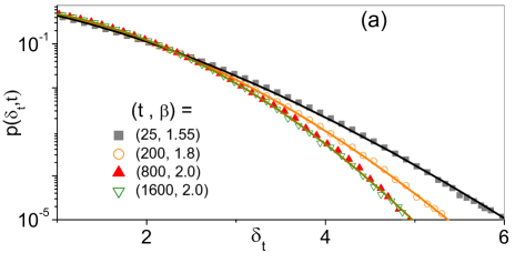
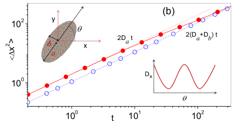
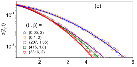
Figure 1: Overdamped 2D ellipsoidal particle of semi-axes $a=0.5$ and $b=0.05$ diffusing in a homogeneous medium with Langevin Eqs. (7)-(9): (a), (c) displacement pdf’s for different initial orientations [uniform $\theta(0)$ distribution in (a), and $\theta(0)=0$ in (c)] and increasing observation times, $t$, see legends; (b) $\langle\Delta x^{2}\rangle$ vs. $t$ for the initial conditions (i.c.) of (a) (empty symbols) and (c) (filled symbols). Simulation parameters are: $D_{a}=1$, $D_{b}=(b/a)D_{a}$ and $D_{r}=0.01$. Asymptotic diffusion in (b) follows the normal diffusion law, $2Dt$ with $D=(D_{a}+D_{b})/2$ (dashed line), independent of the i.c. At very short times, the diffusion constant depends on $\theta(0)$ (see sketch). The pdf’s have been fitted by means of Eq. (17) for $D$ fitting the large-$t$ simulation data of (b) and $\beta$ as reported in the legends.

Despite their apparent simplicity, the analytical solution of the Langevin Eqs. (7)-(9) is rather cumbersome Pecora ; Franosch . The diffusion properties of a typical ellipsoidal particle are summarized in Fig. 1. The mean square displacement, $\langle\Delta x^{2}(t)\rangle$, plotted in panel (b) as a function of the observation time $t$, was first computed under assuming a uniform distribution of $\theta(0)$. This initial condition (i.c.) was justified with the practical difficulty of measuring the particle instantaneous orientation and with the isotropy of the suspension medium. The resulting asymptotic diffusion constant, numerically determined as

$$D=\lim_{t\to\infty}\langle\Delta x^{2}(t)\rangle/2t,$$

agrees with the expected value, $D=(D_{a}+D_{b})/2$, obtained by averaging $D_{ij}(\theta)$ in Eq. (9) with respect to the isotropic equilibrium distribution of $\theta$. This result is indeed an effect of our choice for the i.c. of $\theta$. A stochastic average over a uniform $\theta(0)$ distribution is equivalent to imposing isotropic particle’s diffusion, that is establishing Einstein law at any time. In contrast, by setting $\theta(0)=0$, the numerical data for $\langle\Delta x^{2}\rangle$ versus $t$, also shown in Fig. 1(b), bridge two linear laws with different diffusion constant: $D=D_{a}$ for $t\ll\tau$ and $D=(D_{a}+D_{b})/2$ for $t\gg\tau$.

More revealing are the distributions of the unidirectional displacements, $\Delta x$, for increasing observation times, $t$, plotted in panels (a) and (c), respectively for a uniform initial angular distribution and $\theta(0)=0$. As first theoretically predicted by Prager Prager and numerically confirmed by the authors of Ref. Franosch , for both i.c. the rescaled displacement pdf’s do approach the Gaussian profile of Fickian diffusion with half-variance $D=(D_{a}+D_{b})/2$, but only for $t\gg\tau$, that is well after the anisotropic-isotropic crossover took place. Most remarkably, for $\theta(0)=0$, in panel (c), the displacement distributions approach a Gaussian profile both for $t\ll\tau$ and $t\gg\tau$, each with the corresponding half-variance $D$ shown in panel (b), respectively, $D_{a}$ and $(D_{a}+D_{b})/2$. The short-$t$ “reentrant” Gaussian distribution does not appear in panel (a), due to the randomized i.c.. The explanation of this behavior is simple. In panel (c), the particle’s long axis was initially oriented parallel to the $x$ axis, $\theta(0)=0$. Therefore, it started diffusing in the $x$ direction like a one dimensional Brownian particle, with diffusion constant $D_{a}$. Subsequently, angular fluctuations mixed diffusion along the two symmetry axes with time constant $\tau$. This argument can be extended to any choice of $\theta(0)$: based on Eq. (9), the short-$t$ diffusion constant is expected to be $D=(1/2)[(D_{a}+D_{b})+(D_{a}-D_{b})\cos\theta(0)]$, see inset of Fig. 1(b). Of course, the i.c. only influence the anisotropic diffusion regime at short $t$.

There is only one characteristic time scale in this model, namely, the angular relaxation time, $\tau=1/D_{\theta}$. However, normal diffusion turns out to set in for shorter observation times, $t\sim\tau$, than the displacement Gaussian statistics. To explain this behavior, we notice that during the transient time, $\tau$, a maximum mean square displacement, $2D_{a}\tau$, occurs parallel to the major axis; observing the same displacement in the perpendicular direction would take a larger time, $\tau_{*}=\tau(D_{a}/D_{b})$. The onset of the Gaussian $\Delta x$ statistics is thus delayed to larger observation times with $t>\tau_{*}$.

In conclusion, this simple model of equilibrium Brownian motion exhibits NGND. On decreasing the observation time, $t$, the rescaled displacement distribution in a fixed laboratory direction, changes from Gaussian for $t\gg\tau$, to a leptokurtic distribution with fat exponential tails for $t\sim\tau$, independently of the i.c.. This behavior is consistent with the phenomenological picture of Sec. II. This is apparent in the case of uniform initial orientation. Normal diffusion is ensured by the fact that, after the particle has taken a step $\Delta x_{i}$ at the discrete time $t_{i}=i\Delta x$, it will next take a step $\pm\Delta x_{j}$ at time $t_{j}$, with equal probability. On the contrary, the step lengths $\Delta x_{i}$ and $\Delta x_{j}$ are correlated for $|t_{j}-t_{i}|<\tau$. Indeed, the effective half-width of the diffusing particle parallel to the $x$ axis, varies randomly between $b$ at $\theta=0,\pi$ and $a$ at $\theta=\pm\pi/2$. Accordingly, the particle’s instantaneous diffusion constant fluctuates between $D_{a}$ and $D_{b}$; its fluctuations are exponentially time correlated with time constant $\tau$. As discussed in Sec. II, this leads to a rescaled pdf, $p(\delta_{t},t)$, with positive excess kurtosis.

IV Diffusion of a Janus Particle

We consider next the case of a pointlike particle undergoing persistent Brownian motion, namely, a 2D artificial microswimmer. Typical artificial microswimmers are Brownian particles capable of self-propulsion in an active medium Granick ; Muller . Like in the foregoing section, the suspension medium can be taken homogeneous, isotropic and highly viscous. Such particles are designed to harvest environmental energy by converting it into kinetic energy. The simplest class of artificial swimmers investigated in the literature are the so-called Janus particles (JP), mostly spherical colloidal particles with two differently coated hemispheres, or “faces” Marchetti ; Gompper . Recently, artificial micro- and nanoswimmers of this class have been the focus of pharmaceutical (e.g., smart drug delivery smart ) and medical research (e.g., robotic microsurgery Wang ). Relevant to the present work is the observation that their function is governed, in time and space, by their diffusive properties through complex environments, which are often spatially patterned Bechinger or confined ourPRL .

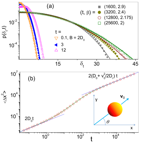
Figure 2: Symmetric Janus particle diffusing in a homogeneous medium with $D_{0}=1$, $v_{0}=1$, $D_{\theta}=0.01$, and uniform distributions of the particle’s initial position and orientation, Eqs. (10)-(11): (a) displacement pdf’s at different observation times, $t$; (b) diffusion law, $\langle\Delta x^{2}\rangle$ vs. $t$. The numerical data agree well with the analytical law of Eq. (12) (solid curve); the normal diffusion limits at large and short $t$, Eqs. (13) and (14), are drawn for a comparison (dashed lines); the pdf’s in (a) have been fitted by means of Eq. (17) with $D$ fitting the large-$t$ data in (b) and an appropriate choice of $\beta$ (see legend). The pdf’s with $\beta=2$ at the shortest and largest $t$, panel (a), are Gaussian curves with half-variance $D_{0}$ and $D_{0}+D_{s}$, respectively.

The overdamped dynamics of a pointlike active JP can be formulated by means of two translational and one rotational Langevin equation

$$\dot{x} = v_{0}\cos\theta+\xi_{x}(t),~{}~{}~{}\dot{y}=v_{0}\sin\theta+\xi_{y}(t),$$ (10)

$$\dot{\theta} = \xi_{\theta}(t),$$ (11)

where $x$ and $y$ are the coordinates of the particle’s center of mass, and the self-propulsion velocity has constant modulus, $v_{0}$, and orientation $\theta$, taken with respect to the $x$ axis, see sketch in Fig. 2(b). The translational noises in the $x$ and $y$ directions, $\xi_{x}(t)$ and $\xi_{y}(t))$, and the rotational noise, $\xi_{\theta}(t)$, are stationary, independent, delta-correlated Gaussian noises, $\langle\xi_{i}(t)\xi_{j}(0)\rangle=2\delta_{ij}D_{i}\delta(t)$ with $i,j=x,y,\theta$. The noise strengths $D_{x}=D_{y}=D_{0}$ (isotropic translational fluctuations) and $D_{\theta}$ are assumed here to be unrelated for generality (e.g., to account for different self-propulsion mechanisms ourPRL ). The reciprocal of $D_{\theta}$ is the correlation (or angular persistence) time, $\tau$, of the self-propulsion velocity. For simplicity, we ignore chiral effects due to unavoidable fabrication defects Wang ; Loewen ; chiral1 . It is worthy comparing the Langevin Eqs. (7)-(8) and (10)-(11): for the ellipsoidal particle anisotropy is geometric, i.e., due to its elongated shape, whereas, for a pointlike JP anisotropy is dynamical, i.e., associated with the instantaneous orientation of its self-propulsion velocity.

A detailed analytical treatment of the Langevin Eqs. (10)-(11) is to be found in Ref. Franosch_SciRep . The unidirectional diffusion of a free JP in 2D reads Golestanian07 ; Loewen09 ; chiral2 ,

$$\langle\Delta x^{2}(t)\rangle=2(D_{0}+D_{s})t+D_{s}\tau(e^{-|t|/\tau}-1),$$ (12)

which approaches the Einstein law,

$$\langle\Delta x^{2}(t)\rangle=2(D_{0}+D_{s})t,$$ (13)

only for $t\gg\tau$. Here, the unidirectional diffusion constant, $D$, consists of two distinct contributions, a translational, $D_{0}$, and a self-propulsion term, $D_{s}=v_{0}^{2}/2D_{\theta}$. Instead, for short observation times Eq. (12) tends to

$$\langle\Delta x^{2}(t)\rangle=2D_{0}t,$$ (14)

that is, to the normal diffusion law of a passive particle with $v_{0}=0$. The analytical law of Eq. (12) and its normal limits for large and small observation times compare well with our simulation results in Fig. 2(b).

The displacement distribution, $p(\delta_{t},t)$, exhibits a Gaussian profile both for $t\to 0$ and $t\to\infty$, but with different half-variances, respectively $D_{0}$ and $D=D_{0}+D_{s}$, see Fig. 2(a). The crossover between these two Gaussian limits is characterized by platykurtic transient pdf’s with fast decaying tails. Experimental evidence of this phenomenon has been reported in Ref. Loewen2 . In the limit $t\to 0$, the displacement distributions become sensitive to the particle’s initial orientation. For a uniform distribution of $\theta(0)$, shown in Fig. 2(a), the rescaled pdf’s approach a Gaussian function with half-variance $D_{0}$, as to be expected for an isotropic persistent Brownian motion in the ballistic regime, $t\ll\tau$. However, for a fixed value of $\theta(0)$, say, $\theta(0)=0$, the pdf is still a Gaussian with the same half-variance, $D_{0}$, but its center moves to higher $\Delta x$ values, with $\langle\Delta x(t)\rangle=v_{0}t$ sperm (not shown). For intermediate observation times, $t\simeq\tau$, the displacement pdf’s develop two symmetric maxima a distance of the order of the persistence length, $\Delta x\sim v_{0}\tau$, from their centers Loewen2 .

The different nature of the diffusion transients of ellipsoidal and active JP’s can be easily explained in terms of the coarse grained model of Sec. II. The orientation of a JP is time correlated; from Eqs. (10)-(11), $\langle\cos\theta(t)\cos\theta(0)\rangle=\langle\sin\theta(t)\sin\theta(0)\rangle=(1/2)\exp(-|t|/\tau)$. This implies that both the orientation and the length of the discrete steps in the $x$ direction, $\Delta x_{i}$ are time correlated; given any pair of steps, $\Delta x_{i}$ and $\Delta x_{j}$, both their time correlations vanish asymptotically only for $|t_{j}-t_{i}|\gg\tau$. However, on comparing panels (a) and (b) of Fig. 2 we notice the existence of a rather wide range of observation times, where $\langle\Delta x^{2}(t)\rangle$ has approached a linear function of $t$, Eq. (13), while the rescaled $\Delta x$ distributions are still apparently platykurtic.

The platykurtic nature of this transient is consistent with the coarse grained model of Sec. II, because the angular correlation of the self-propulsion velocity vector amounts to an oscillatory behavior of $D_{i}-\langle D_{i}\rangle$, a necessary condition to observe a negative excess kurtosis, $\mu_{x}<0$. It remains to explain why, like in Sec. III, the onset of normal diffusion anticipates the onset of the Gaussian $\Delta x$ statistics. We know Loewen2 that the self-propulsion mechanism of Eqs. (10)-(11) is responsible for the non-Gaussian profile of $p(\delta_{t})$, an effect mitigated by the translational noise as long as $2D_{0}t>l_{\theta}^{2}$, where $l_{\theta}=v_{0}\tau$ is the JP persistence length. Therefore, the Gaussian statistics of the unidirectional JP displacements is expected to emerge only for $t>\tau_{*}$, with $\tau_{*}=\tau(D_{s}/D_{0})$. Note that in the simulations of Fig. 2 we set $\tau_{*}>\tau$.

The results presented in this section lead us to conclude that we are in the presence of another manifestation of the NGND phenomenon.

V Transient Displacement Distributions

As mentioned in Sec. I, the notion of NGND is commonly associated with the existence of a wide interval of observation times, where diffusion follows a normal law with fixed constant, $D$, and the rescaled displacement distribution, $p(\delta_{t})$, decays (almost) exponentially independently of $t$. The exponential to Gaussian crossover is hardly accessible to direct observation Granick1 . In the low dimensional systems investigated here, instead, such a transition takes place over a relatively narrower $t$ interval, which led us to look for a phenomenological function $p(\delta_{t},t)$ fitting our simulation data from transient up asymptotic $t$ values.

Contrary to the diffusing diffusivity models, where the limiting Laplace and Gaussian distributions are functions of the sole diffusion constant, $D$, a more realistic fitting procedure needs at least one additional parameter, $\beta$, to capture the $t$-dependence of the transient pdf’s. Inspired by the numerical findings of Secs. III and IV, we started from the compressed exponential function

$$p(\delta_{t})=p_{0}e^{-(\delta_{t}/\delta_{0})^{\beta}},$$ (15)

where $\beta\geq 1$. The scaling factor, $\delta_{0}$, and the normalization constant, $p_{0}$, have been computed by imposing the conditions

$$\int_{0}^{\infty}p(\delta_{t})d\delta_{t}=1,~{}~{}~{}\int_{0}^{\infty}\delta_{t}^{2}p(\delta_{t})d\delta_{t}=2D,$$ (16)

to obtain the one-parameter ad hoc fitting function,

$$p_{\beta}(\delta_{t})=\frac{\beta}{\Gamma(\frac{1}{\beta})^{\frac{3}{2}}}\left[\frac{\Gamma(\frac{3}{\beta})}{2D}\right]^{\frac{1}{2}}\exp\left[-\left(\frac{\delta_{t}^{2}}{2D}\frac{\Gamma(\frac{3}{\beta})}{\Gamma(\frac{1}{\beta})}\right)^{\frac{\beta}{2}}\right].$$ (17)

This function has been derived phenomenologically starting from the standard stretched exponential distribution, $p_{\beta}(\delta_{t})=A\exp(-B\delta_{t}^{\beta})$. The constants $A$ and $B$ have then be determined by normalizing $p_{\beta}(\delta_{t})$ to one and ensuring that its second moment yields $\langle\delta_{t}^{2}\rangle=2D$ for any value of the free parameter $\beta$. In view of its derivation, the heuristic distribution (17) may apply also to the transients of microscopically non-Gaussian diffusion models nonG1 ; nonG2 ; nonG3 . The fitting parameter $\beta$ is allowed to vary with $t$; it assumes values in the range $1\leq\beta\leq 2$ for leptokurtic distributions (positive excess kurtosis) and $\beta\geq 2$ for platykurtic distributions (negative excess kurtosis).

The fits of the pdf’s drawn in panels (a),(c) of Figs. 1 and (a) of Fig. 2 have been generated from Eq. (17) by setting $D$ equal to the diffusion constants that best fitted the large-$t$ diffusion data in the respective panels (b) and, then, computing $\beta$ to get the best fit of the rescaled displacement distributions at different $t$. The same fitting procedure has been applied in Figs. 3 and 4 of the forthcoming sections.

Our phenomenological formula (17) fits rather closely the numerical pdf’s reported in Secs. III and IV, at least for sufficiently large observation times. As a matter of fact, the heuristic argument leading to the fitting function $p_{\beta}(\delta_{t})$ assumes normal diffusion at any $t$. This is consistent with the diffusive dynamics of the ellipsoidal Brownian particle with isotropic i.c., displayed in Figs. 1(a)-(b). However, this cannot be the case, for instance, of the active JP of Fig. 2, whose diffusion law for $t<\tau$ clearly deviates from the asymptotic law of Eq. (13). A comparison with the simulation output confirms that the proposed fitting procedure works well for both systems in the transient regime, $t>\tau$.

VI Diffusion in a Time Modulated Channel

In most numerical and experimental investigations Granick1 ; Granick2 ; Bhatta ; Sung1 ; Sung2 ; Granick3 the transient distributions of $\delta_{t}$ are presented as sort of universal functions, $p(\delta_{t})$, which decay with (almost) exponential law independently of $t$. Sometimes the transient interval is so wide that the exponential-Gaussian crossover is not accessible to direct observation. The question then rises as to what extent the low dimensional systems addressed in this work may share that property. In the notation of Sec. V, this corresponds to determining conditions for the fitting parameter $\beta$ to be constant with $\beta\neq 2$ (non-Gaussian transient) over a wide range of $t$. Note that in the models of Secs. III and IV the onset of the normal diffusion and the Gaussian statistics regimes, which delimit the NGND transient, are governed by the sole angular relaxation time $\tau$ ($\tau_{*}$ being proportional to $\tau$). In the standard formalism of the central limit theorem this would correspond to saying that the higher cumulants of the displacement distribution vanish slower with the observation time than the second moment approaches its linear growth Feller . In this regard, more interesting are systems where the NGND transients are delimited by two distinct time constants.

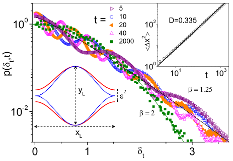
Figure 3: Diffusion of a pointlike overdamped particle in a randomly fluctuating channel, Eq. (19) with $\varepsilon(t)$ representing the Ornstein-Uhlenbeck process of Eq. (20). Simulation parameters are: $y_{L}=1$, $x_{L}=\pi$, $D_{0}=1$, $D_{\varepsilon}=3$, $\tau=50$, and random $x(0)$, $y(0)$ and $\varepsilon(0)$. In the main panel, rescaled displacement pdf’s are shown for increasing observation times, $t$, in the normal diffusion regime, see data for $\langle\Delta x^{2}\rangle$ vs. $t$ in the inset. The fitting $\beta$ values have been obtained from Eq. (17) with $D=0.335$. At short $t$, the statistics of our data is not good enough to resolve the $t$ dependence of $\beta$.

A study case is represented by the diffusion of a standard Brownian particle in a confined geometry chemphyschem , the simplest example being a chainlike structure of cavities connected by narrow pores PRR . In 2D, the dynamics of an overdamped symmetric Brownian particle in a channel is modeled by two simple Langevin equations

$$\dot{x}=\xi_{x}(t),~{}~{}~{}\dot{y}=\xi_{y}(t),$$ (18)

where $x$ and $y$ are the coordinates of the particle’s center of mass and the translational fluctuations $\xi_{x}(t)$ and $\xi_{y}(t)$ are zero-mean, white Gaussian noises with autocorrelation functions $\langle\xi_{i}(t)\xi_{j}(0)\rangle=2\delta_{i,j}D_{0}\delta(t)$ and $i,j=x,y$. The strength of $\xi_{i}(t)$ coincides with the free-particle diffusion constant, $D_{0}$, which is typically proportional to the temperature of the suspension fluid. However, contrary to Secs. III and IV, the particle is now confined to diffuse inside a narrow corrugated channel with axis oriented along $x$ and symmetric walls, $y=\pm w(x,t)$. Following Refs. chemphyschem , we assumed for simplicity the sinusoidally modulated channel half-width

$$w(x,t)=(y_{L}/2)[\varepsilon^{2}+(1-\varepsilon^{2})\sin^{2}(\pi x/x_{L})].$$ (19)

Here $y_{L}$ and $x_{L}$ are respectively the maximum width and the length of the unit channel cell, sketched in Fig. 3, and $\varepsilon^{2}y_{L}$ is the fluctuating width of the pores located at $x{\rm mod}(x_{L})=0$. In the case of a pointlike particle, hydrodynamic effects PNAS can be ignored. Moreover, let the width of the channel pores be time modulated without affecting the particle’s free diffusion constant, $D_{0}$, for instance, by applying a tunable external gating potential. Therefore, when integrating the Langevin Eq. (18), we neglected the particle radius with respect to $x_{L}$ and $y_{L}$ (pointlike particle approximation) and imposed reflecting boundary conditions at the walls ourPRL .

In Ref. PRR we considered the case when $\varepsilon(t)$ is an Ornstein-Uhlenbeck process

$$\dot{\varepsilon}=-\varepsilon/\tau+\sqrt{D_{\varepsilon}/\tau^{2}}~{}\xi_{\varepsilon}(t),$$ (20)

where $\xi_{\varepsilon}(t)$ is another Gaussian zero-mean valued noise, independent of $\xi_{x}(t)$ and $\xi_{y}(t)$ and delta-correlated, $\langle\xi_{\varepsilon}(t)\xi_{\varepsilon}(0)\rangle=2\delta(t)$. The channel pores open and close randomly in time with average width $\langle\varepsilon^{2}\rangle y_{L}$, where $\langle\varepsilon^{2}\rangle$ coincides with the variance of $\varepsilon(t)$, $D_{\varepsilon}/\tau=(\pi/2)\langle|\varepsilon|\rangle^{2}$.

This channel model manifests prominent NGND, as illustrated in Fig. 3. The displacement distributions are Gaussian for both very short (not shown, see Ref. PRR ) and asymptotically long observation times. Indeed, the particle diffuses freely with constant $D_{0}$ inside each channel’s cell for $t<\tau_{L}$, with $\tau_{L}=x_{L}^{2}/8D_{0}$, before escaping into an adjacent cell after a mean exit time $\tau_{0}=\tau_{L}/\langle|\varepsilon|\rangle$ PRR . For $t\gg\tau_{0}$, the $x$ directed diffusion process can thus be described as a random walker with spatial step $x_{L}$ and time constant $\tau_{0}$; memory of the i.c. adopted in our simulations is completely erased. The ensuing mean square displacement then follows the Einstein law with approximated diffusion constant $D=x_{L}^{2}/2\tau_{0}$ JCP137 . The displacement distribution assumes its asymptotic Gaussian profile only for observation times much larger than the correlation time of the pore fluctuations, $t\gg\tau$. In the simulations of Fig. 3, we set $\tau\gg\tau_{0}$, which thus defines a NGND transient interval, $(\tau_{0},\tau)$, where diffusion is normal, but the displacement distributions are non-Gaussian. By taking such interval wide enough, the transient pdf’s, $p(\delta_{t},t)$, grow insensitive to $t$, and so do the fitted $\beta$ values. This way, we mimic the situation reported in the literature Granick1 ; Granick2 ; Bhatta ; Sung1 ; Sung2 ; Granick3 for more complex systems.

This prescription for NGND control is independent of the detailed statistics of the pore fluctuations. For instance, one can consider the case of a periodically time modulated pore width with

$$\varepsilon(t)=\delta_{\varepsilon}\cos(t/\tau).$$ (21)

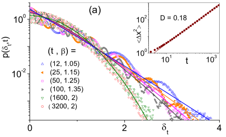
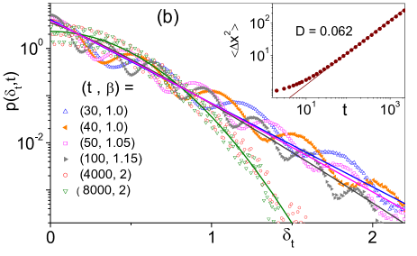
Figure 4: Diffusion of a pointlike overdamped particle in a corrugated channel, Eq. (19), with $\varepsilon(t)$ representing the periodically time modulation of Eq. (21). Simulation parameters are: $y_{L}=1$, $x_{L}=\pi$, $D_{0}=1$, $\delta^{2}_{\varepsilon}=0.03$, and (a) $\tau=100$, (b) $\tau=500$. The initial conditions were set by imposing uniform distributions of the particle’s initial position and $\varepsilon(t)$ initial phase. In the main panels, rescaled displacement pdf’s are plotted for increasing $t$, in the normal diffusion regime. The values of $\beta$ in the legend have been obtained by fitting Eq. (17) with $D$ computed numerically from the asymptotes, $\langle\Delta x^{2}\rangle=2Dt$, drawn in the insets.

The simulation data plotted in Fig. 4(a) confirm the existence of the NGND transient interval $(\tau_{0},\tau)$, where $\tau$ is now the period of the sinusoidal function $\varepsilon(t)$ of Eq. (21) and $\langle\varepsilon^{2}\rangle=\delta_{\varepsilon}^{2}/2=(\pi^{2}/8)\langle|\varepsilon|\rangle^{2}$. For a quantitative comparison, in Figs. 3 and 4(a) $\langle\varepsilon^{2}\rangle$ have been assigned the same value, so that for the simulation parameters of Fig. 4 both time scales, $\tau_{0}$ and $\tau$, are larger by approximately the same factor two.

The NGND phenomenon in Fig. 4(a) is apparent. The rescaled pdf’s shown there are clearly non-Gaussian. Fat oscillating tails arise for $t>\tau$, as an effect of the spatial periodicity of the channel. Indeed, the oscillation period of the plotted distributions is of the order $x_{L}/\sqrt{t}$. This effect, detectable also in Figs. 3 and 4(b), plays here a marginal role. Indeed, on disregarding such oscillations, the tails of the non-Gaussian distributions can still be fitted by the function of Eq. (17) for an appropriate choice of the free parameter $\beta$.

However, in Fig. 4(a) and in contrast with Fig. 3, the deterministic nature of the pore time modulation allowed us to resolve a weak $t$-dependence of $\beta$, without increasing the statistical accuracy of our simulation runs. It is important to remark that such a residual $t$-dependence of the transient rescaled pdf’s can be further suppressed by widening the transient interval $(\tau_{0},\tau)$. An example is shown in panel (b) of Fig. 4, where the simulation parameters are the same as in panel (a), except for the modulation period, $\tau$, which is five times larger. We remark that, for the simple model at hand, this result is analytically predictable upon reformulating the particle’s dynamics in the dimensionless units, $x\to x/x_{L}$, $y\to y/x_{L}$ and $t\to t/\tau$.

VII Diffusion in Convection Rolls

We finally address the reasons why transients under NGND conditions can be either lepto- or platykurtic. In Secs. III and IV we looked at two simple models, which exhibit distributions of the one or the other type, respectively, with $1\leq\beta\leq 2$ and $\beta\geq 2$. We consider now a slightly more complicated 2D system, which can undergo both transients, depending on the choice of its dynamical parameters. The numerical analysis of its diffusion properties will help us shed light on the different microscopic mechanisms responsible for these two type of transients, thus justifying the generalization of the NGND notion proposed in this work.

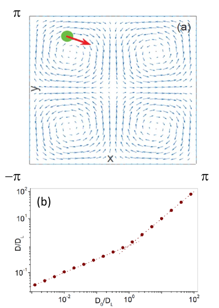
Figure 5: Diffusion in the periodic convective flow pattern of Eq. (22): (a) Flow cell unit consisting of four counter-rotating subcells; (b) The asymptotic diffusion constant, $D$ vs. $D_{0}$: the numerical data (dots) are compared with the analytical prediction discussed in the text, see Eq. (24). The stream function parameters are $U_{0}=1$ and $L=2\pi$, and the diffusion scale is $D_{L}=U_{0}L/2\pi$.

To this purpose we investigated the diffusion of a pointlike overdamped particle of coordinates $x$ and $y$, suspended in a stationary planar laminar flow with periodic center-symmetric stream function Gollub1 ; Gollub2 ; Rosen ; Pomeau ; Saintillan ; Vulpiani ; Neufeld .

$$\psi(x,y)=({U_{0}L}/{2\pi})\sin({2\pi x}/{L})\sin({2\pi y}/{L}),$$ (22)

where $U_{0}$ is the maximum advection speed and $L$ the wavelength of the flow unit cell. The ensuing particle’s dynamics can be formulated in terms of two driven Langevin equations,

$$\dot{x}=u_{x}+\xi_{x}(t),~{}~{}~{}~{}\dot{y}=u_{y}+\xi_{y}(t),$$ (23)

with the vector $(u_{x},u_{y})=(\partial_{y},-\partial_{x})\psi$ representing the local advection velocity. As illustrated in Fig. 5(a), this defines four counter-rotating flow subcells, also termed convection rolls. The translational noises, $\xi_{i}(t)$ with $i=x,y$ are stationary, independent Gaussian noises with auto-correlation functions $\langle\xi_{i}(t)\xi_{j}(0)\rangle=2D_{0}\delta_{ij}\delta(t)$. They can be regarded as modeling homogeneous, isotropic thermal fluctuations. In our simulations, the flow parameters, $U_{0}$ and $L$ were kept fixed, as they define the natural length and time units, $L$ and $\Omega_{L}^{-1}=L/2\pi U_{0}$, respectively. Therefore, the only tunable parameter left is the noise strength, $D_{0}$. Having in mind a stationary system, we assumed uniform distributions of the initial particle’s coordinates, $x(0)$ and $y(0)$. Indeed, due to the incompressibility of $(u_{x},u_{y})$, in the presence of translational noise, a particle’s trajectory eventually fills up the flow unit cell uniformly. To this regard, we remind that, in the absence of noise, the advection period tends to diverge as the closed trajectory of a dragged particle runs close the subcell boundaries Weiss ; hence, for $D_{0}=0$ the particle gets trapped in a convection roll Rosen ; Pomeau ; Neufeld .

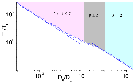
Figure 6: Diffusion mechanisms in the periodic flow pattern of Eq. (22): mean first-exit time, $T_{D}$, vs. thermal noise, $D_{0}$. Convection flow parameters are $U_{0}=1$ and $L=2\pi$. The asymptotic solid lines on the left and right are respectively $T_{0}$ and $T_{0}/4$, with $T_{0}$ given in Eq. (25); the horizontal dashed line represents the advection period, $T_{L}$. Three $D_{0}$ intervals. shaded in different colors, are separated by $D_{*}$, obtained by imposing $T_{D}=T_{L}$, and $D_{L}$, defined in Fig. 5. In each interval, the range of $\beta$ is reported for reader’s convenience; no NGND was detected for $D_{0}>D_{L}$.

Particle transport in such a flow pattern has been studied under diverse conditions and a rich phenomenology has emerged Gollub1 ; Gollub2 ; Rosen ; Pomeau ; Saintillan ; Vulpiani ; Neufeld . We focus here on the Brownian diffusion of a passive particle under the simultaneous action of translational fluctuations and advective drag. A first important feature of this system is illustrated in Fig. 5(b), where we plotted the dependence of the asymptotic diffusion constant, $D$, on the noise intensity (and particle’s no-flow diffusion constant), $D_{0}$. The mean square displacement is an asymptotically linear function of time for any choice of $D_{0}$. However, on increasing $D_{0}$, the diffusion constant, $D$, changes from

$$D=\kappa\sqrt{D_{L}D_{0}},$$ (24)

for $D_{0}<D_{L}$ (advective diffusion), to $D=D_{0}$, for $D_{0}>D_{L}$ (thermal diffusion), an abrupt crossover occurring at $D_{0}\simeq D_{L}$, with $D_{L}=U_{0}L/2\pi$ RR2 . The constant $\kappa$ depends on the geometry of the flow cells Rosen ; Pomeau ; for a 2D array of square counter-rotating convection rolls, $\kappa\simeq 1.06$ Rosen . This property can be explained with the fact that for $D<D_{L}$ the spatial diffusion occurs along the separatrices delimiting the four subcells of the stream function, $\psi(x,y)$, of Fig. 5(a). Stated otherwise, the diffusion process is regulated by the advection velocity field ourPOF . Vice versa, for $D_{0}>D_{L}$ the effects of advection on the particle’s diffusion become negligible. Not surprisingly, we detected NGND only for $D_{0}<D_{L}$.

The diffusion process is governed by two competing mechanisms: (i) Particle’s circulation inside the counter-rotating subcells of $\psi(x,y)$. The corresponding vorticity, $\nabla\times{\mathbf{u}}=-\nabla^{2}\psi$, has a maximum, $\Omega_{L}=2\pi U_{0}/L$, at the center of the subcells. This defines the time scale, $T_{L}=2\pi/\Omega_{L}$, for the advection period, that is an estimate of the average time taken by advection to drag the particle around a convection roll; (ii) Diffusion across the convection rolls. The mean first-exit time, $T_{D}$, of a Brownian particle out of a unit convection cell of $\psi(x,y)$, can be easily computed for $D_{0}\gg D_{L}$ simply by ignoring advection Gardiner ,

$$T_{0}=\frac{1}{D_{0}}\left(\frac{L}{2\pi}\right)^{2}\left(\frac{4}{\pi}\right)^{4}~{}\sum_{m,n}^{(\rm odd)}\frac{1}{m^{2}}\frac{1}{n^{2}}\frac{1}{m^{2}+n^{2}},$$ (25)

where the summation is restricted to the odd values of $m$ and $n$. In the opposite limit, $D_{0}\ll D_{L}$, $T_{D}$ is just one fourth of $T_{0}$, because, as anticipated above, at very low noise levels, the exit process consists of a slow activation mechanism, which takes the particle from the center of a subcell to its boundaries, followed by a relatively faster flow-driven propagation along the grid formed by the subcell separatrices.

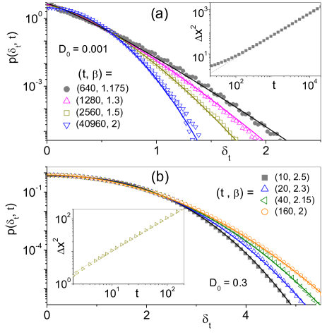
Figure 7: Leptokurtic, $D_{0}<D^{*}$ (a), and platykurtic transients, $D^{*}<D_{0}<D_{L}$ (b), in a periodic array of 2D convection rolls. $D_{0}$, $t$ and $\beta$ are reported in the legends; convection flow parameters are $U_{0}=1$ and $L=2\pi$. All transient pdf’s were taken in the regime of normal diffusion, see insets.

Thanks to thermal fluctuations, the Brownian particle jumps from roll to roll, thus diffusing in the $x,y$ plane. Its coarse-grained motion can be modeled as a discrete random walker with time constant $T_{D}$ Gardiner . Therefore, for large observation times, $t>T_{D}$, the particle executes normal diffusion.

For the simulation parameters adopted in Fig. 6, the crossover between low- and high-noise estimates of $T$, respectively $T_{D}=T_{0}$ and $T_{D}=T_{0}/4$, occurs in the region of advective diffusion, $D_{0}<D_{L}$. More remarkably, it appears to correspond to the condition, $T_{D}=T_{L}$, namely, when the two competing time scales of the particle’s dynamics inside a convection roll coincide. Such a condition defines a unique $D_{0}$ value, $D_{*}$, which splits the advective diffusion domain into two distinct subdomains, respectively, $D_{0}<D_{*}$ and $D_{*}<D_{0}<D_{L}$.

Numerical simulation clearly shows evidence of NGND for $t>T_{D}$, in close analogy with the models of Secs. III and IV, except for an important peculiarity: The transient displacement distributions displayed in Fig. 7, turn out to be leptokurtic, with $1\leq\beta\leq 2$, for $D_{0}<D_{*}$, and platykurtic, with $\beta\geq 2$, for $D_{*}<D_{0}<D_{L}$. This can be explained with the fact that here the displacement length correlation, see Sec. II, is dominated by thermal noise in the lower $D_{0}$ interval, where $T_{D}>T_{L}$, and by advection in the larger $D_{0}$ interval, where $T_{L}>T_{D}$. Accordingly, in the formulation of Secs. III and IV, the role of transient time, $\tau$, is played respectively by $T_{D}$ for $D_{0}<D_{*}$ and by $T_{L}$ for $D_{0}>D_{*}$.

For $D_{*}\ll D_{0}<D_{L}$, the onset of normal diffusion and the exponential-Gaussian transitions are thus regulated by two distinct time scales, respectively, $T_{0}$ and $T_{L}$. Indeed, the slowest time modulation of the particle’s dynamics is due to the advective drag inside the convection rolls. By generalizing our discussion for the NGND of a free JP, Sec. IV, we conclude that such a rotational dynamics must be responsible for the negative excess kurtosis of the unidirectional particle’s displacements reported in Fig. 7(b). The range of the $\beta$ values, fitted according to the procedure of Sec. V, is shown in Fig. 6 for each $D_{0}$ interval.

In conclusion, the NGND transients of this model can change from leptokurtic to platykurtic simply by raising the strength of the internal noise. Most remarkably, this and related diffusive systems are easily accessible to direct experimental demonstration Gollub2 ; Saintillan .

VIII Conclusions

In this work we have investigated NGND transients Granick1 ; Granick2 ; Bhatta ; Sung1 ; Sung2 ; Granick3 in low dimensional stochastic processes. These become apparent when the Einstein law, which characterizes normal diffusion, sets in for observation times, $t$, shorter than the asymptotic Gaussian displacement statistics, predicted by the central limit theorem. A wide class of low dimensional systems manifest NGND under the condition that their local dynamics is subjected to time correlated modulations.

Time modulation can affect the effective particle geometry (e.g., its cross-section in the diffusion direction, Sec. III), its dynamics (e.g., its isotropic self-propulsion mechanism, Sec. IV), or its confinement geometry (e.g., the cross-section of the directed channel containing the particle, Sec. VI). In all cases discussed here the system’s modulation is time correlated with time constant, $\tau$, larger than any other microscopic dynamical time scale. We then noticed that NGND becomes more prominent when the onset times of normal diffusion and the Gaussian displacement statistics are well separated, with the former much lower than the latter. This situation is well illustrated by the fluctuating narrow channel of Sec. VI, where normal diffusion occurs for $t$ larger than the mean pore crossing time and the Gaussian statistics sets in for $t$ larger that the tunable correlation time of the pore modulation.

In low dimensional systems, NGND features exhibit a smooth dependence on the observation time. The transient rescaled displacement distributions are not “universal” over large $t$ intervals, in sharp contrast with the extended disordered systems first studied in the literature Granick1 ; Granick2 ; Bhatta ; Sung1 ; Sung2 ; Granick3 . To quantify the $t$-dependence of the transient pdf’s we introduced an ad hoc fitting function, $p_{\beta}(\delta_{t})$, which, by construction, reproduces the normal diffusion law, with diffusion constant obtained by direct observation, and fits the numerical curves $p(\delta_{t},t)$ by tuning only one free parameter, $\beta$. Actually, in Sec. VI we noticed that by increasing the gap between the two distinct time scales defining the transient interval, the $t$-dependence of $\beta$ is suppressed, with $\beta$ tending to one (Laplace distribution). This situation closer resembles the current description of the NGND phenomenon in complex systems.

However, NGND in low dimensional systems has the advantage of being easily controllable by tuning the time modulation of the microscopic dynamics. For instance, the two simplest models discussed here, the free ellipsoidal and Janus particles, exhibit remarkably different transient distributions, respectively with fat, $1\leq\beta\leq 2$, and thin tails, $\beta\geq 2$. Platykurtic transient distributions are peculiar to systems with rotational modulation of the diffusion process, because, as discussed in Sec. II, this can cause negative time correlations of the unidirectional displacement lengths; hence the negative values of the excess kurtosis.

This conclusion is corroborated by Brownian diffusion in the periodic array of 2D convection rolls discussed in Sec. VII. In contrast with the elementary models of Secs. III and IV, there the physical mechanism determining the transient time varies depending on the strength of the thermal fluctuations. At low temperatures, the transient dynamics of the particle is governed by isotropic random jumps from convection roll to convection roll, largely insensitive to the details of its trajectory inside the individual rolls. On the contrary, at higher temperatures, but still in the advective diffusion regime, roll jumping grows faster compared with the circulation inside the rolls; transients are then dominated by a rotational dynamics, which causes a negative excess kurtosis of the particle’s displacements.

We conclude now mentioning a number of open issues we intend to address in the next future.

(i) We showed that low-dimensional systems exhibit NGND transients for observation times not too much larger than their largest intrinsic relaxation time. It remains to be seen how one can make such transient time intervals wider, for instance, by means of a hierarchy of additional stochastic degrees of freedom.

(ii) We wonder to what extent our discussion of discrete NGND in Sec. II is related to the formalism of the large deviations theory LDT . This might provide an alternate phenomenological description of the NGND transients, also applicable to higher dimensional systems.

(iii) NGND transients in laminar flows are of great relevance in microfluidics. This results reviewed in Sec.7 will be published in a more detailed report to appear soon JFM . We showed that leptokurtic (platykutic) transients are an effect of the mostly thermal (advective) tracer’s diffusion. The question then rises as how this explanation translates in the cases of turbulent flows, a recurrent problem in biological systems.

(iv) Finally, it is conceivable that persistent NGND transients impact how active micro-swimmers interact with each other or with confining walls or other obstacles, to form all kinds of clustered structures. The implications of such a mechanism in the technology of active matter need further investigation.

- (1) B. Wang, S. M. Anthony, S. C. Bae, and S. Granick, Anomalous yet Brownian, Proc. Natl. Acad. Sci. U.S.A. 106, 15160 (2009).
- (2) B. Wang, J. Kuo, C. Bae, and S. Granick, When Brownian diffusion is not Gaussian, Nat. Mater. 11, 481 (2012).
- (3) S. Bhattacharya, D. K. Sharma, S. Saurabh, S. De, A. Sain, A. Nandi, and A. Chowdhury, Plasticization of poly(vinylpyrrolidone) thin films under ambient humidity: Insight from single-molecule tracer diffusion dynamics, J. Phys. Chem. B 117, 7771 (2013).
- (4) J. Kim, C. Kim, and B. J. Sung, Simulation study of seemingly Fickian but heterogeneous dynamics of two dimensional colloids, Phys. Rev. Lett. 110, 047801 (2013).
- (5) G. Kwon, B. J. Sung, and A. Yethiraj, Dynamics in crowded environments: Is non-Gaussian Brownian diffusion normal? J. Phys. Chem. B 118, 8128 (2014).
- (6) J. Guan, B. Wang, and S. Granick, Even hard-sphere colloidal suspensions display Fickian yet non-Gaussian diffusion, ACS Nano 8, 3331 (2014).
- (7) C. Gardiner, Stochastic Methods: A Handbook for the Natural and Social Sciences (Springer, Berlin, 2009).
- (8) E. R. Weeks, J. C. Crocker, A. C. Levitt, A. Schofield, D. A. Weitz, Three-dimensional direct imaging of structural relaxation near the colloidal glass transition, Science 287, 627 (2000).
- (9) J. D. Eaves and D. R. Reichman, Spatial dimension and the dynamics of supercooled liquids, Proc. Natl. Acad. Sci. U.S.A. 106, 15171 (2009).
- (10) K. C. Leptos, J. S. Guasto, J. P. Gollub, A. I. Pesci, and R. E. Goldstein, Dynamics of enhanced tracer diffusion in suspensions of swimming eukaryotic microorganisms, Phys. Rev. Lett. 103, 198103 (2009).
- (11) W. K. Kegel and A. van Blaaderen, Direct observation of dynamical heterogeneities in colloidal hard-sphere suspensions, Science 287, 290 (2000).
- (12) P. Chaudhuri, L. Berthier, and W. Kob, Universal nature of particle displacements close to glass and jamming transitions, Phys. Rev. Lett. 99, 060604 (2007).
- (13) S. K. Ghosh, A. G. Cherstvy, D. S. Grebenkov and R. Metzler, Anomalous, non-Gaussian tracer diffusion in crowded two-dimensional environments, New J. Phys. 18, 013027 (2016).
- (14) W. He, H. Song, Y. Su, L. Geng, B. J. Ackerson, H. B. Peng, and P. Tong, Dynamic heterogeneity and non-Gaussian statistics for acetylcholine receptors on live cell membrane, Nat. Comm. 7, 11701 (2016).
- (15) M. V. Chubynsky and G. W. Slater, Diffusing diffusivity: A model for anomalous, yet Brownian, diffusion, Phys. Rev. Lett. 113, 098302 (2014).
- (16) A. G. Cherstvy and R. Metzler, Anomalous diffusion in time-fluctuating non-stationary diffusivity landscapes, Phys.Chem.Chem.Phys. 18, 23840 (2016).
- (17) R. Jain and K. L. Sebastian, Diffusion in a crowded, rearranging environment, J. Phys. Chem. B 120, 3988 (2016).
- (18) R. Jain and K. L. Sebastian, Diffusing diffusivity: A new derivation and comparison with simulations, J. Chem. Sci. 129, 929 (2017).
- (19) N. Tyagi and B. J. Cherayil, Non-Gaussian Brownian diffusion in dynamically disordered thermal environments, J. Phys. Chem. B 121, 7204 (2017).
- (20) L. Luo and M. Yi, Non-Gaussian diffusion in static disordered media, Phys. Rev. E 97, 042122 (2018).
- (21) A. V. Chechkin, F. Seno, R. Metzler, and I. M. Sokolov, Brownian yet non-Gaussian diffusion: From superstatistics to subordination of diffusing diffusivities, Phys. Rev. X 7, 021002 (2017).
- (22) J. Slezak, R. Metzler, and M. Magdziarz, Superstatistical generalised Langevin equation: non-Gaussian viscoelastic anomalous diffusion, New J. Phys. 20, 023026 (2018).
- (23) Y. Li, F.Marchesoni, D. Debnath, and P. K. Ghosh, Non-Gaussian normal diffusion in a fluctuating corrugated channel, Phys. Rev. Res. 1, 033003 (2019).
- (24) P. Hänggi and F. Marchesoni, Artificial Brownian motors: Controlling transport on the nanoscale, Rev. Mod. Phys. 81, 387 (2009).
- (25) R. Lipowsky, Generic interactions of flexible membranes, in Handbook of Biological Physics, (R. Lipowsky and E. Sackmann, editors) Vol. 1, Ch. 11 (Elsevier, 1995).
- (26) P. S. Burada, P. Hänggi, F. Marchesoni, G. Schmid, and P. Talkner, Diffusion in confined geometries, ChemPhysChem 10, 45 (2009).
- (27) X. Yang, C. Liu, Y. Li, F. Marchesoni, P. Hänggi, and H. P. Zhang, Hydrodynamic and entropic effects on colloidal diffusion in corrugated channels, Proc. Natl. Acad. Sci. U.S.A. 114, 9564 (2017).
- (28) V. Sposini, A. V. Chechkin, F. Seno, G. Pagnini, and R. Metzler, Random diffusivity from stochastic equations: Comparison of two models for Brownian yet non-Gaussian diffusion, New J. Phys. 20, 043044 (2018).
- (29) L. Luo and M. Yi, Quenched trap model on the extreme landscape: The rise of subdiffusion and non-Gaussian diffusion, Phys. Rev. E 100, 042136 (2019).
- (30) L. Luo and M. Yi, Ergodicity recovery of random walk in heterogeneous disordered media, Chin. Phys. B 29, 050503 (2020)
- (31) for a review, see H. C. Berg, Random Walk in Biology (Princeton University Press, 1984).
- (32) F. Perrin, Mouvement brownien d’un ellipsoide - I. Dispersion diélectrique pour des molécules ellipsoidales, J. Phys. Radium V, 497 (1934); Mouvement Brownien d’un ellipsoide (II). Rotation libre et dépolarisation des fluorescences. Translation et diffusion de molécules ellipsoidales ibid. VII, 1 (1936).
- (33) Y. Han, A. M. Alsayed, M. Nobili, J. Zhang, T. C. Lubensky, and A. G. Yodh, Brownian motion of an ellipsoid, Science 314, 626 (2006).
- (34) P. E. Kloeden and E. Platen, Numerical Solution of Stochastic Differential Equations (Springer, 1992).
- (35) S. R. Aragón and R. Pecora General theory of dynamic light scattering from cylindrically symmetric particles with translational‐rotational coupling, J. Chem. Phys. 82, 5346 (1985).
- (36) S. Leitmann, F. Höfling, and T. Franosch, Dynamically crowded solutions of infinitely thin Brownian needles, Phys Rev E 96, 012118 (2017).
- (37) S. Prager, Interaction of rotational and translational diffusion, J. Chem. Phys. 23, 2404 (1955).
- (38) S. Jiang and S. Granick (Eds.), Janus particle synthesis, self-assembly and applications (RSC Publishing, Cambridge, 2012).
- (39) A. Walther and A. H. E. Müller, Janus particles: Synthesis, self-assembly, physical properties, and applications, Chem. Rev. 113, 5194 (2013).
- (40) M. C. Marchetti, J. F. Joanny, S. Ramaswamy, T. B. Liverpool, J. Prost, M. Rao, and R. A. Simha, Hydrodynamics of soft active matter, Rev. Mod. Phys. 85, 1143 (2013).
- (41) J. Elgeti, R. G. Winkler, and G. Gompper, Physics of microswimmers, single particle motion and collective behavior: a review, Rep. Progr. Phys. 78, 056601 (2015).
- (42) see e.g. Smart Drug Delivery System, edited by A. D. Sezer (IntechOpen, 2016). DOI: 10.5772/60475
- (43) J. Wang, Nanomachines: Fundamentals and Applications (Wiley-VCH, Weinheim, 2013).
- (44) G. Volpe, I. Buttinoni, D. Vogt, H.-J. Kümmerer, and C. Bechinger, Microswimmers in patterned environments, Soft Matter, 7, 8810 (2011).
- (45) P. K. Ghosh, V. R. Misko, F. Marchesoni, and F. Nori, Self-propelled Janus particles in a ratchet: Numerical simulations, Phys. Rev. Lett. 110, 268301 (2013).
- (46) S. vanTeeffelen and H. Löwen, Dynamics of a Brownian circle swimmer, Phys. Rev. E 78, 020101(RC) (2008).
- (47) D. Debnath, P. K. Ghosh, Y. Li, F. Marchesoni, and B. Li, Diffusion of eccentric microswimmers, Soft Matt. 12, 2017 (2016).
- (48) C. Kurzthaler, S. Leitmann, and T. Franosch, Intermediate scattering function of an anisotropic active Brownian particle, Sci. Rep. 6, 36702 (2016).
- (49) J. R. Howse, R. A. L. Jones, A. J. Ryan, T. Gough, R. Vafabakhsh, and R. Golestanian, Self-motile colloidal particles: From directed propulsion to random walk Phys. Rev. Lett. 99, 048102 (2007).
- (50) B. ten Hagen, S. van Teeffelen, H. Löwen, Non-Gaussian behaviour of a self-propelled particle on a substrate, Condens. Matter Phys. 12, 725 (2009).
- (51) X. Ao, P. K. Ghosh, Y. Li, G. Schmid, P. Hänggi, and F. Marchesoni, Diffusion of chiral Janus particles in a sinusoidal channel, EPL 109, 10003 (2015).
- (52) X. Zheng, B. ten Hagen, A. Kaiser, M. Wu, H. Cui, Z. Silber-Li, and H. Löwen, Non-Gaussian statistics for the motion of self-propelled Janus particles: experiment versus theory, Phys. Rev. E 88, 032304 (2013).
- (53) D. Debnath, P. K. Ghosh, V. R. Misko, Y. Li, F. Marchesoni, and F. Nori, Enhanced motility in a binary mixture of active nano/microswimmers, Nanoscale 12, 9717 (2020).
- (54) W. Feller, An Introduction To Probability Theory And Its Applications, Vol. 2 (Wiley, New York, 1991).
- (55) L. Bosi, P. K. Ghosh, and F. Marchesoni, Analytical estimates of free Brownian diffusion times in corrugated narrow channels, J. Chem. Phys. 137, 174110 (2012).
- (56) T. H. Solomon and J. P. Gollub, Chaotic particle transport in time-dependent Rayleigh-Bénard convection, Phys. Rev. A 38, 6280 (1988).
- (57) T. H. Solomon and I. Mezić, Uniform resonant chaotic mixing in fluid flows, Nature (London) 425, 376 (2003).
- (58) M. N. Rosenbluth, H. L. Berk, I. Doxas, and W. Horton, Effective diffusion in laminar convective flows, Phys. Fluids, 30, 2636 (1987).
- (59) W. Young, A. Pumir, and Y. Pomeau, Anomalous diffusion of tracer in convection rolls, Phys. Fluids A 1, 462 (1989).
- (60) Y.-N. Young and M. J. Shelley, Stretch-coil transition and transport of fibers in cellular flows, Phys. Rev. Lett. 99, 058303 (2007); H. Manikantan and D. Saintillan, Subdiffusive transport of fluctuating elastic filaments in cellular flows, Phys. Fluids 25, 073603 (2013).
- (61) A. Sarracino, F. Cecconi, A. Puglisi, and A. Vulpiani, Nonlinear response of inertial tracers in steady laminar flows: Differential and absolute negative mobility, Phys. Rev. Lett. 117, 174501 (2016).
- (62) C. Torney and Z. Neufeld, Transport and aggregation of self-propelled particles in fluid flows, Phys. Rev. Lett. 99, 078101 (2007)
- (63) N. O. Weiss, The expulsion of magnetic flux by eddies, Proc. Roy. Soc. A293, 310 (1966).
- (64) Y. Li, L. Li, F. Marchesoni, D. Debnath, and P. K. Ghosh, Active diffusion in convection rolls, Phys. Rev. Res. 2, 013250 (2020).
- (65) Q. Yin, Y. Li, F. Marchesoni, T. Debnath, and P. K. Ghosh, Exit times of a Brownian particle out of a convection roll, Phys. Fluids 32, 092010 (2020).
- (66) J. Feng and T. G. Kurtz, Large Deviations for Stochastic processes, Mathematical Surveys and Monographs, Vol. 131 (Am. Math. Society, 2006)
- (67) Q. Yin, Y. Li, B. Li, F. Marchesoni, S. Nayak, and P. K. Ghosh, Diffusion transients in convection rolls, to be published in J. Fluid Mech. (2021) DOI:10.1017/jfm.2020.1127.