Non-tensorial Gravitational Wave Background in NANOGrav 12.5-Year Data Set

Abstract

We perform the first search for an isotropic non-tensorial gravitational-wave background (GWB) allowed in general metric theories of gravity in the North American Nanohertz Observatory for Gravitational Waves (NANOGrav) 12.5-year data set. By modeling the GWB as a power-law spectrum, we find strong Bayesian indication for a spatially correlated process with scalar transverse (ST) correlations whose Bayes factor versus the spatially uncorrelated common-spectrum process is $107\pm 7$, but no statistically significant evidence for the tensor transverse, vector longitudinal and scalar longitudinal polarization modes. The median and the $90\%$ equal-tail amplitudes of ST mode are $\mathcal{A}_{\mathrm{ST}}=1.06^{+0.35}_{-0.28}\times 10^{-15}$, or equivalently the energy density parameter per logarithm frequency is $\Omega_{\mathrm{GW}}^{\mathrm{ST}}=1.54^{+1.21}_{-0.71}\times 10^{-9}$, at frequency of 1/year.

Introduction. The direct detection of gravitational waves (GWs) from compact binary coalescences Abbott et al. (2016a, 2019a, 2020a) has marked the beginning of a new era of GW astronomy and provides a powerful tool to test gravitational physics in the strong-field regime Abbott et al. (2019b, 2020b). The current ground-based GW detectors are sensitive to GWs at frequencies of $10\sim 10^{4}$ Hz Abbott et al. (2016b). As a complementary tool, the stable millisecond pulsars are natural galactic scale GW detectors that are sensitive in nano-Hertz frequency band, opening a new window to explore the Universe. By monitoring the spatially correlated fluctuations induced by GWs on the time of arrivals (TOAs) of radio pulses from an array of pulsars Sazhin (1978); Detweiler (1979); Foster and Backer (1990), a pulsar timing array (PTA) seeks to detect the very low frequency GWs which might be sourced by the inspiral of supermassive black hole binaries (SMBHBs) Jaffe and Backer (2003); Sesana et al. (2008, 2009), the first-order phase transition Witten (1984); Hogan (1986), the scalar-induced GWs Saito and Yokoyama (2009); Yuan et al. (2019a, b), etc. The null-detection of GWs by PTAs has successfully constrained various astrophysical scenarios, such as cosmic strings Lentati et al. (2015); Arzoumanian et al. (2018); Yonemaru et al. (2020), continuous GWs from individual SMBHBs Zhu et al. (2014); Babak et al. (2016); Aggarwal et al. (2018), GW memory effects Wang et al. (2015); Aggarwal et al. (2019), primordial black holes Chen et al. (2020), and stochastic GW backgrounds (GWBs) of a power-law spectrum Lentati et al. (2015); Shannon et al. (2015); Arzoumanian et al. (2018). However, the direct detection of GWs by PTAs remains a key task in astrophysical experiments, and is hopefully achieved in the next few years Siemens et al. (2013); Taylor et al. (2016).

Recently, the North American Nanohertz Observatory for Gravitational Waves (NANOGrav) collaboration has reported strong evidence for a stochastic common-spectrum process, which is significantly preferred over an independent red-noise process in each pulsar Arzoumanian et al. (2020). The characteristic strain of this process is described by a power-law model, $h_{c}(f)\propto f^{-2/3}$, corresponding to the GW emission from inspiraling SMBHBs. NANOGrav announced there was no statistically significant evidence for quadrupolar spatial correlations. Moreover, this process shows moderately negative evidence for monopolar and dipolar correlations, which may come from the reference clock and solar system ephemeris (SSE) anomalies, respectively. Lacking definitive evidence for quadrupolar spatial correlations Arzoumanian et al. (2020), NANOGrav argued that it is inconclusive to claim a detection of GWB consistent with general relativity (GR), and the origin of this process remains controversial.

Even though there is no definitive evidence for tensor transverse (TT) correlations predicted by GR in the NANOGrav 12.5-year data set, it does not exclude the possibility of other GW polarization modes allowed in general metric theories of gravity. In fact, a most general metric gravity theory can allow two vector modes and two scalar modes besides the two tensor modes, and these different modes have distinct correlation patterns Lee et al. (2008); Chamberlin and Siemens (2012); Gair et al. (2015); Boîtier et al. (2020), allowing the GW detectors to explore them separately. To figure out whether the signal originates from a GWB or not, it is necessary to fit the data with all possible correlation patterns. In this letter, we perform the first Bayesian search for the stochastic GWB signal modeled by a power-law spectrum with all the six polarization modes in the NANOGrav 12.5-year data set. Such a power-law spectrum of GWB can be produced by the inspiraling SMBHBs by assuming circular orbits whose decays are dominated by GWs and neglecting higher moments Cornish et al. (2018). We find the Bayes factor in favor of a spatially correlated common-spectrum process with the scalar transverse (ST) correlations versus the spatially uncorrelated common-spectrum process (UCP) is $107\pm 7$ which indicates that strong Bayesian indication for the ST correlations in the NANOGrav 12.5-year data set.

Detecting GWB Polarizations with a PTA. The radio pulses from pulsars, especially millisecond pulsars, arrive at the Earth at extremely steady rates, and pulsar timing experiments exploit this regularity. The geodesics of the radio waves can be perturbed by GWs, inducing the fluctuations in the TOAs of radio pulses Sazhin (1978); Detweiler (1979). The presence of a GW will manifest as the unexplained residuals in the TOAs after subtracting a deterministic timing model that accounts for the pulsar spin behavior and the geometric effects due to the motion of the pulsar and the Earth Sazhin (1978); Detweiler (1979). By regularly monitoring TOAs of pulsars from an array of the ultra rotational stable millisecond pulsars Foster and Backer (1990) and using the expected form for cross correlations of a signal between pulsars in the array, it is feasible to discriminate the GW signal from other systematic effects, such as clock or SSE errors.

For any two pulsars ($a$ and $b$) in a PTA, the cross-power spectral density of the timing residuals induced by a GWB at frequency $f$ will be Lee et al. (2008); Chamberlin and Siemens (2012); Gair et al. (2015)

$$S_{ab}(f)=\sum_{P}\frac{h_{c,P}^{2}}{12\pi^{2}f^{3}}\Gamma^{P}_{ab}(f),$$ (1)

where $h_{c}^{P}(f)$ is the characteristic strain and the sum is over all the six possible GW polarizations which may be presented in a general metric gravity theory, namely $P=+,\times,x,y,l,b$. Here, “$+$” and “$\times$” denote the two different spin-2 transverse traceless polarization modes; “$x$” and “$y$” denote the two spin-1 shear modes; “$l$” denotes the spin-0 longitudinal mode; and “$b$” denotes the spin-0 breathing mode. The overlap function $\Gamma^{P}_{ab}$ for two pulsars is given by Lee et al. (2008); Chamberlin and Siemens (2012)

$$\Gamma^{P}_{ab}(f)= \frac{3}{8\pi}\int d\hat{\Omega}\left(e^{2\pi ifL_{a}(1+\hat{\Omega}\cdot\hat{p}_{a})}-1\right)\times$$ (2)

$$\left(e^{2\pi ifL_{b}(1+\hat{\Omega}\cdot\hat{p}_{b})}-1\right)F^{P}_{a}(\hat{\Omega})F^{P}_{b}(\hat{\Omega}),$$

where $L_{a}$ and $L_{b}$ are the distance from the Earth to the pulsar $a$ and $b$ respectively, $\hat{\Omega}$ is the propagating direction of the GW, and $\hat{p}$ is the direction of the pulsar with respect to the Earth. The antenna patterns $F^{P}(\hat{\Omega})$ are given by

$$F^{P}(\hat{\Omega})=e^{P}_{ij}(\hat{\Omega})\frac{\hat{p}^{i}\hat{p}^{j}}{2(1+\hat{\Omega}\cdot\hat{p})},$$ (3)

where $e^{P}_{ij}$ is the polarization tensor for polarization mode $P$ Lee et al. (2008); Chamberlin and Siemens (2012). Following Cornish et al. (2018), we define

$$\Gamma^{\mathrm{TT}}_{ab}(f) = \Gamma^{+}_{ab}(f)+\Gamma^{\times}_{ab}(f),$$ (4)

$$\Gamma^{\mathrm{ST}}_{ab}(f) = \Gamma^{b}_{ab}(f),$$ (5)

$$\Gamma^{\mathrm{VL}}_{ab}(f) = \Gamma^{x}_{ab}(f)+\Gamma^{y}_{ab}(f),$$ (6)

$$\Gamma^{\mathrm{SL}}_{ab}(f) = \Gamma^{l}_{ab}(f).$$ (7)

For the $\mathrm{TT}$ and $\mathrm{ST}$ polarization modes, the overlap functions are approximately independent of the distance and frequency and can be analytically calculated by Hellings and Downs (1983); Lee et al. (2008)

$$\Gamma^{\mathrm{TT}}_{ab}(f) = \frac{1}{2}(1+\delta_{ab})+\frac{3}{2}k_{ab}\left(\ln k_{ab}-\frac{1}{6}\right),$$ (8)

$$\Gamma^{\mathrm{ST}}_{ab}(f) = \frac{1}{8}\left(3+4\delta_{ab}+\cos\zeta_{ab}\right),$$ (9)

where $\delta_{ab}$ is the Kronecker delta symbol, $\zeta_{ab}$ is the angle between pulsars $a$ and $b$, and $k_{ab}\equiv(1-\cos\zeta_{ab})/2$. Note that $\Gamma^{\mathrm{TT}}_{ab}$ is known as the Hellings & Downs (HD) Hellings and Downs (1983) or quadrupolar correlations. However, there exist no analytical expressions for the vector longitudinal ($\mathrm{VL}$) and scalar longitudinal ($\mathrm{SL}$) polarization modes, and we calculate them numerically.

PTAs are sensitive to the GWs at frequencies of approximately $10^{-9}\sim 10^{-7}$ Hz, and it is expected that the GWB from a population of inspiraling SMBHBs will be the dominant source in this frequency band Jaffe and Backer (2003); Sesana et al. (2008, 2009). Assuming the binaries are in circular orbits and the orbital decay is dominated by the GW emission, the cross-power spectral density of Eq. (1) can be approximately estimated by Cornish et al. (2018)

$$S_{ab}(f)=\sum_{I={\mathrm{TT},\mathrm{ST},\mathrm{VL},\mathrm{SL}}}\Gamma^{I}_{ab}\frac{\mathcal{A}_{I}^{2}}{12\pi^{2}}\left(\frac{f}{f_{\mathrm{yr}}}\right)^{-\gamma_{I}}f_{\mathrm{yr}}^{-3},$$ (10)

where $\mathcal{A}_{I}$ is the GWB amplitude of polarization mode $I$, and $f_{\mathrm{yr}}=1/\mathrm{year}$. The power-law index $\gamma_{I}$ for the TT polarization is $\gamma_{\mathrm{TT}}=13/3$, and $\gamma_{\mathrm{ST}}=\gamma_{\mathrm{VL}}=\gamma_{\mathrm{SL}}=5$ for other polarizations. The dimensionless GW energy density parameter per logarithm frequency for the polarization mode $I$ is related to $\mathcal{A}_{I}$ by, Thrane and Romano (2013),

$$\Omega_{\mathrm{GW}}^{I}(f)=\frac{2\pi^{2}}{3H_{0}^{2}}f^{2}h_{c,I}^{2}=\frac{2\pi^{2}f_{\mathrm{yr}}^{2}}{3H_{0}^{2}}\mathcal{A}_{I}^{2}\left(\frac{f}{f_{\mathrm{yr}}}\right)^{5-\gamma_{I}},$$ (11)

where $H_{0}$ is the Hubble constant and we take $H_{0}=67.4\,\mathrm{km}\sec^{-1}\mathrm{Mpc}^{-1}$ from Planck 2018 (Aghanim et al., 2020).

PTA data analysis. The NANOGrav collaboration has searched the isotropic GWB in their 12.5-year timing data set Alam et al. (2021) and found strong evidence for a stochastic common-spectrum process but without statistically significant evidence for the TT spatial correlations Arzoumanian et al. (2020). In this letter, we perform the first search for the GWB from the non-tensorial polarization modes in the NANOGrav 12.5-year data set.

Table 1: Parameters and their prior distributions used in the analyses.

parameter	description	prior	comments
White Noise
$E_{k}$	EFAC per backend/receiver system	Uniform $[0,10]$	single-pulsar analysis only
$Q_{k}$[s]	EQUAD per backend/receiver system	log-Uniform $[-8.5,-5]$	single-pulsar analysis only
$J_{k}$[s]	ECORR per backend/receiver system	log-Uniform $[-8.5,-5]$	single-pulsar analysis only
Red Noise
$A_{\rm{RN}}$	red-noise power-law amplitude	log-Uniform $[-20,-11]$	one parameter per pulsar
$\gamma_{\rm{RN}}$	red-noise power-law spectral index	Uniform $[0,7]$	one parameter per pulsar
Uncorrelated Common-spectrum Process (UCP)
$\mathcal{A}_{\mathrm{UCP}}$	UCP power-law amplitude	log-Uniform $[-18,-14]$	one parameter for PTA
$\gamma_{\mathrm{UCP}}$	UCP power-law spectral index	delta function ($\gamma_{\mathrm{UCP}}=13/3$)	fixed
GWB Process
$\mathcal{A}_{\mathrm{TT}}$	GWB amplitude of TT polarization	log-Uniform $[-18,-14]$	one parameter for PTA
$\mathcal{A}_{\mathrm{ST}}$	GWB amplitude of ST polarization	log-Uniform $[-18,-14]$	one parameter for PTA
$\mathcal{A}_{\mathrm{VL}}$	GWB amplitude of VL polarization	log-Uniform $[-19,-15]$	one parameter for PTA
$\mathcal{A}_{\mathrm{SL}}$	GWB amplitude of SL polarization	log-Uniform $[-20,-16]$	one parameter for PTA
BayesEphem
$z_{\rm drift}$ [rad/yr]	drift-rate of Earth’s orbit about ecliptic $z$-axis	Uniform [$-10^{-9},10^{-9}$]	one parameter for PTA
$\Delta M_{\rm jupiter}$ [$M_{\odot}$]	perturbation to Jupiter’s mass	$\mathcal{N}(0,1.55\times 10^{-11})$	one parameter for PTA
$\Delta M_{\rm saturn}$ [$M_{\odot}$]	perturbation to Saturn’s mass	$\mathcal{N}(0,8.17\times 10^{-12})$	one parameter for PTA
$\Delta M_{\rm uranus}$ [$M_{\odot}$]	perturbation to Uranus’ mass	$\mathcal{N}(0,5.72\times 10^{-11})$	one parameter for PTA
$\Delta M_{\rm neptune}$ [$M_{\odot}$]	perturbation to Neptune’s mass	$\mathcal{N}(0,7.96\times 10^{-11})$	one parameter for PTA
PCAi	principal components of Jupiter’s orbit	Uniform $[-0.05,0.05]$	six parameters for PTA

Following NANOGrav Arzoumanian et al. (2020), in our analyses, we use 45 pulsars whose timing baseline is greater than three years. To calculate the longitudinal response functions $\Gamma^{\mathrm{VL}}_{ab}$ and $\Gamma^{\mathrm{SL}}_{ab}$ that are dependent on the pulsar distance from the Earth, we adopt the distance information from the Australia Telescope National Facility (ATNF) pulsar database Manchester et al. (2005). Due to the uncertainty in the pulsar distance measurement, the estimation uncertainty of the overlap function can be $\lesssim 3\%$ for VL mode, and $\lesssim 20\%$ for SL mode. The timing residuals of each single pulsar after subtracting the timing model from the TOAs can be decomposed as Arzoumanian et al. (2016)

$$\delta\bm{t}=M\bm{\epsilon}+F\bm{a}+\bm{n}.$$ (12)

The term $M\bm{\epsilon}$ accounts for the inaccuracies in the subtraction of timing model, where $M$ is the timing model design matrix and $\bm{\epsilon}$ is a vector denoting small offsets for the timing model parameters. The timing model design matrix is obtained through libstempo package which is a python interface to TEMPO2 Hobbs et al. (2006); Edwards et al. (2006) timing software. The term $F\bm{a}$ describes all low-frequency signals, including both the red noise intrinsic to each pulsar and the common red noise signal common to all pulsars (such as a GWB), where $F$ is the Fourier design matrix with components of alternating sine and cosine functions and $\bm{a}$ is a vector giving the amplitude of the Fourier basis functions at the frequencies of $\{1/T,2/T,\cdots,{N_{\text{mode}}}/T\}$ with $T$ the span between the minimum and maximum TOA in the PTA van Haasteren and Vallisneri (2014). Similar to NANOGrav Arzoumanian et al. (2020), we use $30$ frequency components (${N_{\text{mode}}}=30$) for the pulsar intrinsic red noise with a power-law spectrum while using $5$ frequency components (${N_{\text{mode}}}=5$) for the common-spectrum process to mitigate the effect of potentially coupling between the higher-frequency components of common red noise process and the white noise Arzoumanian et al. (2020). The last term $\bm{n}$ describes the timing residuals induced by white noise, including a scale parameter on the TOA uncertainties (EFAC), an added variance (EQUAD), and a per-epoch variance (ECORR) for each backend/receiver system Arzoumanian et al. (2016).

Similar to NANOGrav Arzoumanian et al. (2020), we use the latest JPL SSE, DE438 Folkner and Park (2018), as the fiducial SSE. For verification, we also allow for the BayesEphem Vallisneri et al. (2020) corrections to DE438 to model the SSE uncertainties. However, one should bear in mind that introducing BayesEphem would subtract the power from the putative GWB process and suppress the evidence of the GWB process Vallisneri et al. (2020); Arzoumanian et al. (2020); Pol et al. (2020). To extract information from the data, we perform the Bayesian parameter inferences by closely following the procedure in Arzoumanian et al. (2018, 2020). The parameters of our models and their prior distributions are summarized in Table 1. To reduce the computational costs, in our analyses, we fixed the white noise parameters to their max likelihood values from results released by NANOGrav. We use enterprise Ellis et al. (2020) and enterprise_extension software packages to calculate the likelihood and Bayes factors and use PTMCMCSampler Ellis and van Haasteren (2017) package to do the Markov chain Monte Carlo sampling. To reduce the number of samples needed for the chains to burn in, we use draws from empirical distributions to sample the pulsars’ red noise parameters as was done in Aggarwal et al. (2018); Arzoumanian et al. (2020), with the distributions based on the posteriors obtained from an initial Bayesian analysis that includes only the pulsars’ red noise (i.e. excluding any common red noise process).

Our analysis is mainly based on the Bayesian inference in which the Bayes factor $\mathcal{B}_{10}\equiv\rm{Pr}(\mathcal{D}|\mathcal{M}_{1})/\rm{Pr}(\mathcal{D}|\mathcal{M}_{0})$ is used to quantify the model selection, where $\rm{Pr}(\mathcal{D}|\mathcal{M})$ denotes the probability that the data $\mathcal{D}$ are produced under the assumption of model $\mathcal{M}$. In Kass and Raftery (1995), $\mathcal{B}_{10}\in[20,150]$ and $\mathcal{B}_{10}>150$ respectively correspond to strong and very strong evidence for $\mathcal{M}_{1}$. More optimistically, $\mathcal{B}_{10}\in[10,30]$, $\mathcal{B}_{10}\in[30,100]$, and $\mathcal{B}_{10}>100$ correspond to strong, very strong and extreme evidence for $\mathcal{M}_{1}$ in Lee and Wagenmakers (2014). NANOGrav found strong evidence for a common-spectrum process in the 12.5-year data set and reported the Bayes factors of UCP model versus the pulsar-intrinsic red noise only model to be $10^{4.5}$ with DE438, and $10^{2.4}$ with BayesEphem Arzoumanian et al. (2020). In this letter, the UCP model with fixed spectral index $\gamma_{\mathrm{UCP}}=13/3$ is taken as the fiducial model $\mathcal{M}_{0}$, and the model $\mathcal{M}_{1}$ with $\mathcal{B}_{10}\gg 1$ is supposed to be significantly preferred over the UCP model. We perform analyses on various models by considering different correlation combinations as presented in Eq. (10).

ephemeris	TT	ST	VL	SL
DE438	$4.96(9)$	$107(7)$	$1.94(3)$	$0.373(5)$
BayesEphem	$2.35(3)$	$18.4(7)$	$1.31(2)$	$0.555(7)$

Table 2: The Bayes factors for various models compared to the UCP model with $\gamma=13/3$. The digit in the parentheses gives the uncertainty on the last quoted digit.

Results and discussion. Our results are summarized in Table 2 in which we list the Bayes factors for different models with respect to the UCP model. The Bayes factor of the TT model compared to the UCP model is $4.96\pm 0.09$ with DE438, and $2.35\pm 0.03$ with BayesEphem, indicating no statistically significant evidence for the TT correlations in the data, which is consistent with the results from NANOGrav Arzoumanian et al. (2020). The Bayes factors of VL and SL models compared to the UCP model are smaller than $3$, implying the VL and SL signals are “not worth more than a bare mention” Kass and Raftery (1995). However, the Bayes factor for the ST model versus the UCP model is $107\pm 7$ with DE438, implying strong indication for the ST correlations Kass and Raftery (1995); Lee and Wagenmakers (2014), and we obtain the median and the $90\%$ equal-tail amplitudes as $\mathcal{A}_{\mathrm{ST}}=1.06^{+0.35}_{-0.28}\times 10^{-15}$ or equivalently $\Omega_{\mathrm{GW}}^{\mathrm{ST}}=1.54^{+1.21}_{-0.71}\times 10^{-9}$, at frequency of 1/year. It is known that BayesEphem may absorb a common-spectrum process and weaken the evidence of the GWB process if it exists in the data Vallisneri et al. (2020); Arzoumanian et al. (2020); Pol et al. (2020). Nevertheless, even in the case of BayesEphem, the Bayes factor for the ST model is $18.4\pm 0.7$ which is still significant in the sense of statistics. See the Bayesian posteriors for the ST amplitude $\mathcal{A}_{\mathrm{ST}}$ obtained in the ST model in Fig. 1. Although NANOGrav reported the UCP is more consistent with $\gamma=5.5$ Arzoumanian et al. (2020), we found that such a large Bayes factor for ST model versus the UCP model cannot be explained by the ST spectral index $\gamma_{\rm{ST}}=5$ because the Bayes factor for the ST model versus the UCP model with $\gamma=5.5$ is $96\pm 9$ with DE438. It implies that the preferred ST model is likely attributed to the cross-correlations. Furthermore, we also consider a model that includes a common-spectrum process and an off-diagonal ST-correlated process where all auto-correlation terms are set to zero. The Bayesian amplitude posteriors are shown in Fig. 2 in which the amplitude posterior of the off-diagonal ST-correlated process is significant and comparable to the amplitude posterior of the common-spectrum process, indicating that the large Bayes factor for the ST model should be attributed to the cross-correlations in the NANOGrav 12.5-year data set.

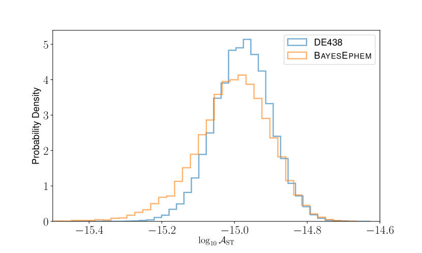
Figure 1: Bayesian posteriors for the ST amplitude $\mathcal{A}_{\mathrm{ST}}$ obtained in the ST model under DE438 and BayesEphem ephemeris schemes, respectively.

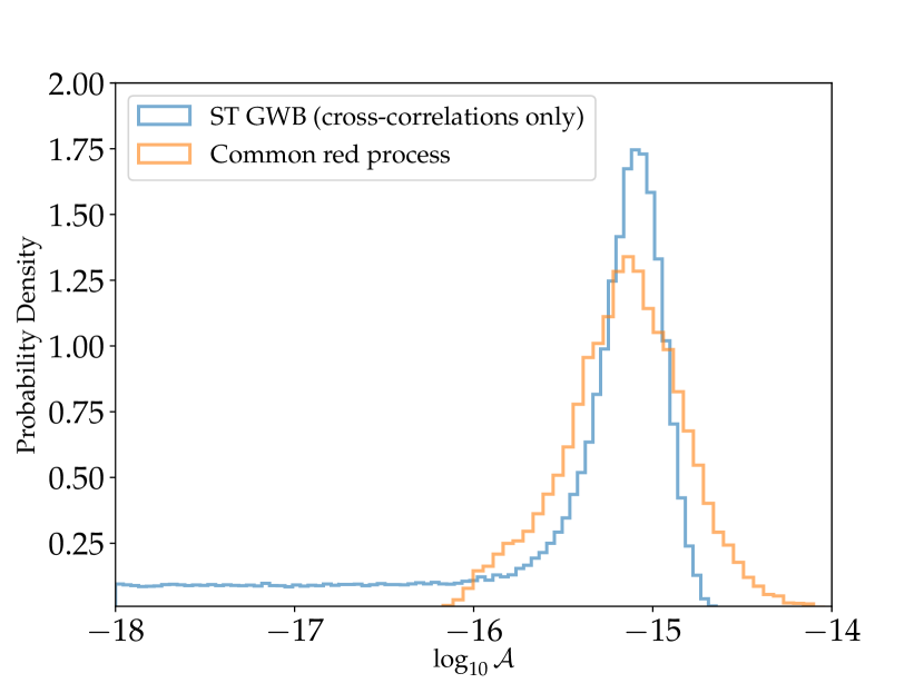
Figure 2: Bayesian amplitude posteriors in a model (with DE438) that includes a common-spectrum process and an off-diagonal ST-correlated process where all auto-correlation terms are set to zero. The posteriors shown here are marginalized to each other.

In addition, we also consider an ST+TT model in which we simultaneously take into account both the ST and TT correlations. The contour plot and the posterior distributions of the ST and TT amplitudes in the ST+TT model are shown in Fig. 3, which implies that the presence of ST correlations is preferred even using BayesEphem, but no significant evidence for additional TT correlations. The amplitude of ST mode from this model with DE438 is $\mathcal{A}_{\mathrm{ST}}=1.02^{+0.36}_{-0.44}\times 10^{-15}$ or equivalently $\Omega_{\mathrm{GW}}^{\mathrm{ST}}=1.45^{+1.21}_{-0.98}\times 10^{-9}$, at frequency of 1/year. This result is consistent with the former one in the ST model.

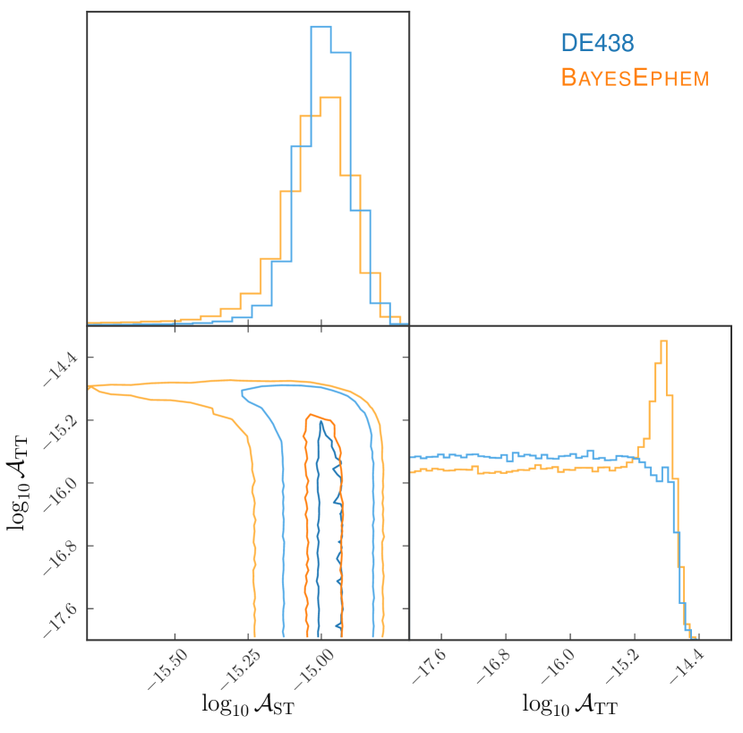
Figure 3: One and two-dimensional marginalized posteriors of ST and TT amplitudes obtained from the ST+TT model under DE438 and BayesEphem ephemeris schemes, respectively. We show both the $1\sigma$ and $2\sigma$ contours in the two-dimensional plot.

To summarize, we find strong Bayesian indication for the ST correlations but no statistically significant evidence for the TT, VL, and SL correlations in the NANOGrav 12.5-year data set. We hope that the future PTA data sets growing in timespan and number of pulsars continue to confirm our results presented in this letter.

Acknowledgments. We would like to thank the anonymous referee for the useful suggestions and comments. We also acknowledge the use of HPC Cluster of ITP-CAS and HPC Cluster of Tianhe II in National Supercomputing Center in Guangzhou. This work is supported by the National Key Research and Development Program of China Grant No.2020YFC2201502, grants from NSFC (grant No. 11975019, 11690021, 11991052, 12047503), Strategic Priority Research Program of Chinese Academy of Sciences (Grant No. XDB23000000, XDA15020701), and Key Research Program of Frontier Sciences, CAS, Grant NO. ZDBS-LY-7009.

References

- Abbott et al. (2016a) B. P. Abbott et al. (LIGO Scientific, Virgo), “Binary Black Hole Mergers in the first Advanced LIGO Observing Run,” Phys. Rev. X6, 041015 (2016a), [erratum: Phys. Rev.X8,no.3,039903(2018)], arXiv:1606.04856 [gr-qc] .
- Abbott et al. (2019a) B.P. Abbott et al. (LIGO Scientific, Virgo), “GWTC-1: A Gravitational-Wave Transient Catalog of Compact Binary Mergers Observed by LIGO and Virgo during the First and Second Observing Runs,” Phys. Rev. X 9, 031040 (2019a), arXiv:1811.12907 [astro-ph.HE] .
- Abbott et al. (2020a) R. Abbott et al. (LIGO Scientific, Virgo), “GWTC-2: Compact Binary Coalescences Observed by LIGO and Virgo During the First Half of the Third Observing Run,” (2020a), arXiv:2010.14527 [gr-qc] .
- Abbott et al. (2019b) B.P. Abbott et al. (LIGO Scientific, Virgo), “Tests of General Relativity with the Binary Black Hole Signals from the LIGO-Virgo Catalog GWTC-1,” Phys. Rev. D 100, 104036 (2019b), arXiv:1903.04467 [gr-qc] .
- Abbott et al. (2020b) R. Abbott et al. (LIGO Scientific, Virgo), “Tests of General Relativity with Binary Black Holes from the second LIGO-Virgo Gravitational-Wave Transient Catalog,” (2020b), arXiv:2010.14529 [gr-qc] .
- Abbott et al. (2016b) Benjamin P. Abbott et al., “Sensitivity of the Advanced LIGO detectors at the beginning of gravitational wave astronomy,” Phys. Rev. D 93, 112004 (2016b), [Addendum: Phys.Rev.D 97, 059901 (2018)], arXiv:1604.00439 [astro-ph.IM] .
- Sazhin (1978) M. V. Sazhin, “Opportunities for detecting ultralong gravitational waves,” Soviet Astronomy 22, 36–38 (1978).
- Detweiler (1979) Steven L. Detweiler, “Pulsar timing measurements and the search for gravitational waves,” Astrophys. J. 234, 1100–1104 (1979).
- Foster and Backer (1990) R. S. Foster and D. C. Backer, “Constructing a pulsar timing array,” Astrophys. J. 361, 300–308 (1990).
- Jaffe and Backer (2003) Andrew H. Jaffe and Donald C. Backer, “Gravitational waves probe the coalescence rate of massive black hole binaries,” Astrophys. J. 583, 616–631 (2003), arXiv:astro-ph/0210148 .
- Sesana et al. (2008) Alberto Sesana, Alberto Vecchio, and Carlo Nicola Colacino, “The stochastic gravitational-wave background from massive black hole binary systems: implications for observations with Pulsar Timing Arrays,” Mon. Not. Roy. Astron. Soc. 390, 192 (2008), arXiv:0804.4476 [astro-ph] .
- Sesana et al. (2009) A. Sesana, A. Vecchio, and M. Volonteri, “Gravitational waves from resolvable massive black hole binary systems and observations with Pulsar Timing Arrays,” Mon. Not. Roy. Astron. Soc. 394, 2255 (2009), arXiv:0809.3412 [astro-ph] .
- Witten (1984) Edward Witten, “Cosmic Separation of Phases,” Phys. Rev. D 30, 272–285 (1984).
- Hogan (1986) C.J. Hogan, “Gravitational radiation from cosmological phase transitions,” Mon. Not. Roy. Astron. Soc. 218, 629–636 (1986).
- Saito and Yokoyama (2009) Ryo Saito and Jun’ichi Yokoyama, “Gravitational wave background as a probe of the primordial black hole abundance,” Phys. Rev. Lett. 102, 161101 (2009), [Erratum: Phys. Rev. Lett.107,069901(2011)], arXiv:0812.4339 [astro-ph] .
- Yuan et al. (2019a) Chen Yuan, Zu-Cheng Chen, and Qing-Guo Huang, “Probing Primordial-Black-Hole Dark Matter with Scalar Induced Gravitational Waves,” (2019a), arXiv:1906.11549 [astro-ph.CO] .
- Yuan et al. (2019b) Chen Yuan, Zu-Cheng Chen, and Qing-Guo Huang, “Log-dependent slope of scalar induced gravitational waves in the infrared regions,” (2019b), arXiv:1910.09099 [astro-ph.CO] .
- Lentati et al. (2015) L. Lentati et al., “European Pulsar Timing Array Limits On An Isotropic Stochastic Gravitational-Wave Background,” Mon. Not. Roy. Astron. Soc. 453, 2576–2598 (2015), arXiv:1504.03692 [astro-ph.CO] .
- Arzoumanian et al. (2018) Z. Arzoumanian et al. (NANOGRAV), “The NANOGrav 11-year Data Set: Pulsar-timing Constraints On The Stochastic Gravitational-wave Background,” Astrophys. J. 859, 47 (2018), arXiv:1801.02617 [astro-ph.HE] .
- Yonemaru et al. (2020) N. Yonemaru et al., “Searching for gravitational wave bursts from cosmic string cusps with the Parkes Pulsar Timing Array,” (2020), 10.1093/mnras/staa3721, arXiv:2011.13490 [gr-qc] .
- Zhu et al. (2014) X.J. Zhu et al., “An all-sky search for continuous gravitational waves in the Parkes Pulsar Timing Array data set,” Mon. Not. Roy. Astron. Soc. 444, 3709–3720 (2014), arXiv:1408.5129 [astro-ph.GA] .
- Babak et al. (2016) Stanislav Babak et al., “European Pulsar Timing Array Limits on Continuous Gravitational Waves from Individual Supermassive Black Hole Binaries,” Mon. Not. Roy. Astron. Soc. 455, 1665–1679 (2016), arXiv:1509.02165 [astro-ph.CO] .
- Aggarwal et al. (2018) K. Aggarwal et al., “The NANOGrav 11-Year Data Set: Limits on Gravitational Waves from Individual Supermassive Black Hole Binaries,” (2018), arXiv:1812.11585 [astro-ph.GA] .
- Wang et al. (2015) J.B. Wang et al., “Searching for gravitational wave memory bursts with the Parkes Pulsar Timing Array,” Mon. Not. Roy. Astron. Soc. 446, 1657–1671 (2015), arXiv:1410.3323 [astro-ph.GA] .
- Aggarwal et al. (2019) K. Aggarwal et al. (NANOGrav), “The NANOGrav 11-Year Data Set: Limits on Gravitational Wave Memory,” (2019), 10.3847/1538-4357/ab6083, arXiv:1911.08488 [astro-ph.HE] .
- Chen et al. (2020) Zu-Cheng Chen, Chen Yuan, and Qing-Guo Huang, “Pulsar Timing Array Constraints on Primordial Black Holes with NANOGrav 11-Year Dataset,” Phys. Rev. Lett. 124, 251101 (2020), arXiv:1910.12239 [astro-ph.CO] .
- Shannon et al. (2015) R.M. Shannon et al., “Gravitational waves from binary supermassive black holes missing in pulsar observations,” Science 349, 1522–1525 (2015), arXiv:1509.07320 [astro-ph.CO] .
- Siemens et al. (2013) Xavier Siemens, Justin Ellis, Fredrick Jenet, and Joseph D. Romano, “The stochastic background: scaling laws and time to detection for pulsar timing arrays,” Class. Quant. Grav. 30, 224015 (2013), arXiv:1305.3196 [astro-ph.IM] .
- Taylor et al. (2016) S.R. Taylor, M. Vallisneri, J.A. Ellis, C.M.F. Mingarelli, T.J.W. Lazio, and R. van Haasteren, “Are we there yet? Time to detection of nanohertz gravitational waves based on pulsar-timing array limits,” Astrophys. J. Lett. 819, L6 (2016), arXiv:1511.05564 [astro-ph.IM] .
- Arzoumanian et al. (2020) Zaven Arzoumanian et al. (NANOGrav), “The NANOGrav 12.5-year Data Set: Search For An Isotropic Stochastic Gravitational-Wave Background,” (2020), arXiv:2009.04496 [astro-ph.HE] .
- Lee et al. (2008) K. J. Lee, F. A. Jenet, and Richard H. Price, “Pulsar Timing as a Probe of Non-Einsteinian Polarizations of Gravitational Waves,” Astrophys. J. 685, 1304–1319 (2008).
- Chamberlin and Siemens (2012) Sydney J. Chamberlin and Xavier Siemens, “Stochastic backgrounds in alternative theories of gravity: overlap reduction functions for pulsar timing arrays,” Phys. Rev. D 85, 082001 (2012), arXiv:1111.5661 [astro-ph.HE] .
- Gair et al. (2015) Jonathan R. Gair, Joseph D. Romano, and Stephen R. Taylor, “Mapping gravitational-wave backgrounds of arbitrary polarisation using pulsar timing arrays,” Phys. Rev. D 92, 102003 (2015), arXiv:1506.08668 [gr-qc] .
- Boîtier et al. (2020) Adrian Boîtier, Shubhanshu Tiwari, Lionel Philippoz, and Philippe Jetzer, “Pulse redshift of pulsar timing array signals for all possible gravitational wave polarizations in modified general relativity,” Phys. Rev. D 102, 064051 (2020), arXiv:2008.13520 [gr-qc] .
- Cornish et al. (2018) Neil J. Cornish, Logan O’Beirne, Stephen R. Taylor, and Nicolás Yunes, “Constraining alternative theories of gravity using pulsar timing arrays,” Phys. Rev. Lett. 120, 181101 (2018), arXiv:1712.07132 [gr-qc] .
- Hellings and Downs (1983) R. w. Hellings and G. s. Downs, “UPPER LIMITS ON THE ISOTROPIC GRAVITATIONAL RADIATION BACKGROUND FROM PULSAR TIMING ANALYSIS,” Astrophys. J. 265, L39–L42 (1983).
- Thrane and Romano (2013) Eric Thrane and Joseph D. Romano, “Sensitivity curves for searches for gravitational-wave backgrounds,” Phys. Rev. D88, 124032 (2013), arXiv:1310.5300 [astro-ph.IM] .
- Aghanim et al. (2020) N. Aghanim et al. (Planck), “Planck 2018 results. VI. Cosmological parameters,” Astron. Astrophys. 641, A6 (2020), arXiv:1807.06209 [astro-ph.CO] .
- Alam et al. (2021) Md F. Alam et al. (NANOGrav), “The NANOGrav 12.5 yr Data Set: Observations and Narrowband Timing of 47 Millisecond Pulsars,” Astrophys. J. Suppl. 252, 4 (2021), arXiv:2005.06490 [astro-ph.HE] .
- Manchester et al. (2005) R N Manchester, G B Hobbs, A Teoh, and M Hobbs, “The Australia Telescope National Facility pulsar catalogue,” Astron. J. 129, 1993 (2005), arXiv:astro-ph/0412641 .
- Arzoumanian et al. (2016) Z. Arzoumanian et al. (NANOGrav), “The NANOGrav Nine-year Data Set: Limits on the Isotropic Stochastic Gravitational Wave Background,” Astrophys. J. 821, 13 (2016), arXiv:1508.03024 [astro-ph.GA] .
- Hobbs et al. (2006) George Hobbs, R. Edwards, and R. Manchester, “Tempo2, a new pulsar timing package. 1. overview,” Mon. Not. Roy. Astron. Soc. 369, 655–672 (2006), arXiv:astro-ph/0603381 [astro-ph] .
- Edwards et al. (2006) Russell T. Edwards, G. B. Hobbs, and R. N. Manchester, “Tempo2, a new pulsar timing package. 2. The timing model and precision estimates,” Mon. Not. Roy. Astron. Soc. 372, 1549–1574 (2006), arXiv:astro-ph/0607664 [astro-ph] .
- van Haasteren and Vallisneri (2014) Rutger van Haasteren and Michele Vallisneri, “New advances in the Gaussian-process approach to pulsar-timing data analysis,” Phys. Rev. D 90, 104012 (2014), arXiv:1407.1838 [gr-qc] .
- Folkner and Park (2018) William M. Folkner and Ryan S. Park, “Planetary ephemeris DE438 for Juno,” Tech. Rep. IOM392R-18-004, Jet Propulsion Laboratory, Pasadena, CA (2018).
- Vallisneri et al. (2020) M. Vallisneri et al. (NANOGrav), “Modeling the uncertainties of solar-system ephemerides for robust gravitational-wave searches with pulsar timing arrays,” (2020), 10.3847/1538-4357/ab7b67, arXiv:2001.00595 [astro-ph.HE] .
- Pol et al. (2020) Nihan S. Pol et al. (NANOGrav), “Astrophysics Milestones For Pulsar Timing Array Gravitational Wave Detection,” (2020), arXiv:2010.11950 [astro-ph.HE] .
- Ellis et al. (2020) Justin A. Ellis, Michele Vallisneri, Stephen R. Taylor, and Paul T. Baker, “Enterprise: Enhanced numerical toolbox enabling a robust pulsar inference suite,” Zenodo (2020).
- Ellis and van Haasteren (2017) Justin Ellis and Rutger van Haasteren, “jellis18/ptmcmcsampler: Official release,” (2017).
- Kass and Raftery (1995) Robert E. Kass and Adrian E. Raftery, “Bayes factors,” Journal of the American Statistical Association 90, 773–795 (1995).
- Lee and Wagenmakers (2014) Michael D. Lee and Eric-Jan Wagenmakers, Bayesian Cognitive Modeling: A Practical Course (Cambridge University Press, 2014).