Spatial Network Decomposition
for Fast and Scalable AC-OPF Learning

Abstract

This paper proposes a novel machine-learning approach for predicting AC-OPF solutions that features a fast and scalable training. It is motivated by the two critical considerations: (1) the fact that topology optimization and the stochasticity induced by renewable energy sources may lead to fundamentally different AC-OPF instances; and (2) the significant training time needed by existing machine-learning approaches for predicting AC-OPF. The proposed approach is a 2-stage methodology that exploits a spatial decomposition of the power network that is viewed as a set of regions. The first stage learns to predict the flows and voltages on the buses and lines coupling the regions, and the second stage trains, in parallel, the machine-learning models for each region. Experimental results on the French transmission system (up to 6,700 buses and 9,000 lines) demonstrate the potential of the approach. Within a short training time, the approach predicts AC-OPF solutions with very high fidelity and minor constraint violations, producing significant improvements over the state-of-the-art. The results also show that the predictions can seed a load flow optimization to return a feasible solution within $0.03\%$ of the AC-OPF objective, while reducing running times significantly.

I Introduction

The AC Optimal Power Flow (AC-OPF) problem is at the core of modern power system operations. It determines the least-cost generation dispatch that meets the demand of the power grid subject to engineering and physical constraints. It is non-convex and NP-hard [1], and the basic block of many applications, including security-constrained OPF [2], [3], security-constrained unit commitment [4], optimal transmission switching [5], capacitor placement [6], and expansion planning [7], among others.

Machine learning has significant potential for real-time AC-OPF applications for a variety of reasons [8]. A machine-learning model can leverage large amount of historical data and deliver extremely fast approximations (compared to an AC-OPF solver). Recent work (e.g., [9, 8]) has indeed shown that machine-learning approaches can predict AC-OPF with high fidelity and minimal constraint violations, using a combination of neural networks and Lagrangian duality. However, the training times and memory requirements of these machine-learning models can be quite significant, which limits their potential applications. Indeed, topology optimization and the stochasticity induced by renewable energy sources may lead to fundamentally different AC-OPF instances and it is unlikely that these approaches would scale to accommodate the wide variety of input configurations encoutered in practice.

This paper explores a fundamentally different avenue: It seeks a scalable machine-learning approach for predicting AC-OPF solutions that can be trained quickly. Such an approach would make it possible to train a machine-learning model quickly to accommodate a new topology or a significant change in the capacity of renewable energy sources. It would also open the possibility of training different machine-learning models for different time periods.

To achieve this goal, the paper proposes a 2-stage machine-learning approach that exploits a spatial decomposition of the power system. The power network is viewed as a set of regions, the first stage learns to predict the flows and voltages on the buses and lines coupling the regions, and the second stage trains, in parallel, the machine-learning models for each region. Experimental results on the French transmission system (up to 6,700 buses and 9,000 lines) demonstrate the potential of the approach. Within a short training time, the approach predicts AC-OPF solutions with very high fidelity and minor constraint violations, producing significant improvements over the state-of-the-art. The results also show that the predictions can seed a load flow optimization to return a feasible solution within $0.03\%$ of the AC-OPF objective, while reducing running times significantly.

To our knowledge, the proposed approach is the first distributed training algorithm for learning AC-OPF for large-scale network topology. It builds on top, and significantly extends, prior work [9, 8] combining machine learning and Lagrangian duality. Most importantly, the 2-stage approach significantly reduces the dimensionality of the learning task, allows the training to be performed in parallel for each region, and dramatically shortens training times, opening new avenues for machine learning in very large-scale system operations. It is also the first approach that can learn AC-OPF on an actual, large-scale tranmission system fast, even on reasonable hardware configurations.

II Related work

Machine learning has attracted significant attention in the power systems community: recent overviews of the various approaches and applications can be found in [10, 11]. In the context of AC-OPF, various approaches have been proposed for learning the active set of constraints [12], [13], [14], [15], [16], imitating the Newton-Raphson algorithm [17], or learning warm-start points for speeding-up the optimization process [18], [19]. Several approaches aim to predict optimal dispatch decisions [20], [21], [22] but these were limited to small-case studies. A load encoding scheme [23] reduces the dimensionality of AC-OPF instances, improving the results of [9, 8]. In the context of DC-OPF, it is worth mentioning the results of [24], [25] that provide formal guarantees on the predictions of neural networks. The application of machine learning to the security-constrained extension of the DC-OPF is presented in [26], [27].

III Preliminaries

The AC Optimal Power Flow Problem

A power network is modeled as an undirected graph $(\mathcal{N},\mathcal{E})$ where $\mathcal{N}$ and $\mathcal{E}$ are the set of buses and transmission lines. The set of generators and loads are denoted by $\mathcal{G}$ and $\mathcal{L}$. The goal of the OPF is to determine the generator dispatch of minimal cost that satisfies the load. The OPF constraints include engineering and physical constraints. The OPF formulation is shown in Figure 1. The power flow equations are expressed in terms of complex power of the form $S\!=\!(p\!+\!jq)$, where $p$ and $q$ denote the active and reactive powers, admittances of the form $Y\!=\!(g\!+\!jb)$, where $g$ and $b$ denote the conductance and susceptance, and voltages of the form $V\!=\!(v\angle\theta)$, with magnitude $v$ and phase angle $\theta$. The formulation uses $v_{i},\theta_{i},p_{i}^{g}$, and $q_{i}^{g}$ to denote the voltage magnitude, phase angle, active power generation, reactive power generation at bus $i$. Moreover, $p^{f}_{ij}$ and $q^{f}_{ij}$ denote the active and reactive power flows associated with line $(i,j)$. The OPF receives as input the demand vectors $p_{i}^{d}$ and $q_{i}^{d}$ for each bus $i$. The objective function captures the cost of the generator dispatch. Typically, $c_{i}(\cdot)$ is a linear or quadratic function. Constraints ($2$), ($3r$), and ($3i$) capture operating bounds for the associated variables. The thermal limit for line $(i,j)$ is captured via constraint ($4$). Constraints ($5r$) and ($5i$) capture Ohm’s Law. Constraints ($6r$) and ($6i$) capture Kirchhoff’s Law.

$$\textbf{minimize}\quad\sum_{i=1}^{\mathcal{|N|}}c_{i}(p_{i}^{g}) 1$$ ()

subject to:

$$\hskip 6.0pt\underline{v}_{i}\leq v_{i}\leq\overline{v}_{i} \!\!\!\!\!\forall i\in{\cal N} 2$$ ()

$$\hskip 6.0pt\underline{p}_{i}^{g}\leq p_{i}^{g}\leq\overline{p}_{i}^{g} \!\!\!\!\!\forall i\in{\cal N} 3r$$ ()

$$\hskip 6.0pt\underline{q}_{i}^{g}\leq q_{i}^{g}\leq\overline{q}_{i}^{g} \!\!\!\!\!\forall i\in{\cal N} 3i$$ ()

$$\hskip 6.0pt(p^{f}_{ij})^{2}+(q^{f}_{ij})^{2}\leq|\overline{S}|_{ij}^{2} \!\!\!\!\!\forall(i,j)\in{\cal E} 4$$ ()

$$\hskip 6.0ptp_{ij}^{f}=g_{ij}v_{i}^{2}-v_{i}v_{j}(b_{ij}\sin(\theta_{i}\text{-}\theta_{j})+g_{ij}\cos(\theta_{i}\text{-}\theta_{j})) \!\!\!\!\!\forall(i,j)\in{\cal E} 5r$$ ()

$$\hskip 6.0ptq_{ij}^{f}=-b_{ij}v_{i}^{2}-v_{i}v_{j}(g_{ij}\sin(\theta_{i}\text{-}\theta_{j})-b_{ij}\cos(\theta_{i}\text{-}\theta_{j})) \!\!\!\!\!\forall(i,j)\in{\cal E} 5i$$ ()

$$\hskip 6.0ptp_{i}^{g}-p_{i}^{d}=\sum_{(i,j)\in\mathcal{E}}p_{ij}^{f} \!\!\!\!\!\forall i\in{\cal N} 6r$$ ()

$$\hskip 6.0ptq_{i}^{g}-q_{i}^{d}=\sum_{(i,j)\in\mathcal{E}}q_{ij}^{f} \!\!\!\!\!\forall i\in{\cal N} 6i$$ ()

Figure 1: The OPF Formulation.

Neural Network Architectures

Neural networks have achieved tremendous success in approximating highly complex, nonlinear mappings in various domains and applications. A Neural Network (NN) consists of a series of layers, the output of each layer being the input to the next layer. The NN layers are often fully connected and the function connecting the layers is given by $\boldsymbol{o}=\pi(\boldsymbol{W}\boldsymbol{x}+\boldsymbol{b}),$ where $\boldsymbol{x}\in\mathbb{R}^{n}$ is the input vector, $\boldsymbol{o}\!\in\!\mathbb{R}^{m}$ the output vector, $\boldsymbol{W}\in\mathbb{R}^{m\times n}$ a weight matrix, and $\boldsymbol{b}\in\mathbb{R}^{m}$ a bias vector. The function $\pi(\cdot)$ is non-linear (e.g., a rectified linear unit (ReLU)).

Notations

The cardinality of set $\mathcal{X}$ is denoted by $|\mathcal{X}|$. $[N]$ represents the set $\{1,2,\dots,N\}$. Vectors are displayed using bold letters and $\boldsymbol{x}$ $=[x_{1},x_{2},...,x_{n}]^{\top}$. The element-wise lower (resp. upper) bound of the vector $\boldsymbol{x}$ is denoted by $\underline{\boldsymbol{x}}$ $(\mbox{resp. }\overline{\boldsymbol{x}})$. In learning algorithms, the prediction for $\boldsymbol{x}$ is denoted by $\hat{\boldsymbol{x}}$.

IV Learning AC-OPF

IV-A OPF Learning Goals

Given loads $(\boldsymbol{p^{d}},\boldsymbol{q^{d}})$, the goal is to predict the optimal setpoints $(\boldsymbol{p^{g}},\boldsymbol{q^{g}})$ of the generators, the bus voltage $\boldsymbol{v}$, and the phase angle difference $\boldsymbol{\Delta\theta}$ of the lines. This task is equivalent to learning the nonlinear, high-dimensional mapping:

$$\mathcal{O}:\mathbb{R}^{2|\mathcal{L}|}\to\mathbb{R}^{\mathcal{|N|}+\mathcal{|E|}+2\mathcal{|G|}} 7$$ ()

which maps the loads onto an optimal AC-OPF solution. The input to the learning task is a dataset

$$\mathcal{D}=\{(\boldsymbol{p^{d}},\boldsymbol{q^{d}})^{t},(\boldsymbol{v},\boldsymbol{\Delta\theta},\boldsymbol{p^{g}},\boldsymbol{q^{g}})^{t}\}_{t=1}^{T}$$

consisting of $T$ instances specifying the inputs and outputs.

IV-B A Lagrangian Dual Model for Learning AC-OPF

One of the challenges of learning mapping $\mathcal{O}$ is the presence of physical and engineering constraints. Ideally, given a NN $\mathcal{O}[\boldsymbol{w}]$ parameterized by weights $\boldsymbol{w}$, the goal is to find the optimal solution $\boldsymbol{w^{*}}$ of the problem:

$$\min_{\boldsymbol{w}} \quad\mathbb{L}_{0}(\boldsymbol{\hat{v}},\boldsymbol{\hat{\theta}},\boldsymbol{\hat{p}^{g}},\boldsymbol{\hat{q}^{g}}) 10$$ ()

s.t. $$\quad(\boldsymbol{\hat{v}},\boldsymbol{\hat{\theta}},\boldsymbol{\hat{p}^{g}},\boldsymbol{\hat{q}^{g}})=\mathcal{O}[\boldsymbol{w}](\boldsymbol{p^{d}},\boldsymbol{q^{d}})$$

$$\quad(\boldsymbol{\hat{v}},\boldsymbol{\hat{\theta}},\boldsymbol{\hat{p}^{g}},\boldsymbol{\hat{q}^{g}},\boldsymbol{\hat{p}^{f}},\boldsymbol{\hat{q}^{f}})\text{ satisfy (\ref{con:2})-(\ref{con:6b}) }$$

where $\mathbb{L}_{0}$ denotes the average norm of the difference between the ground truth and the predictions $\mathbb{L}_{0}(\boldsymbol{\hat{x}})=\frac{1}{T}\sum_{t=1}^{T}\lvert\lvert\boldsymbol{x}^{t}-\boldsymbol{\hat{x}}^{t}\rvert\rvert$ over all training instances, and $(\boldsymbol{\hat{p}^{f}},\boldsymbol{\hat{q}^{f}})$ are computed using constraints ($5r$) and ($5i$). However, it is unlikely that there exist weights $\boldsymbol{w}$ such that the predictions actually satisfy the AC-OPF constraints, since the learning task is a high-dimensional regression task. However, ignoring the constraints entirely leads to predictions that significantly violate the problem constraints as shown in [8, 27]. The approach from [9, 8] addresses this difficulty by using a Lagrangian dual method relying on constraint violations. The violation of a constraint $f(x)\geq 0$ is given by $\nu_{c}(x)=\max\{0,-f(x)\}$, while the violation of $f(x)=0$ is $\nu_{c}(x)=|f(x)|$. Problem ($10$) can then be approximated by

$$\min_{\boldsymbol{w}} \quad\mathbb{L}(\boldsymbol{\lambda},\boldsymbol{w})=\mathbb{L}_{0}(\boldsymbol{\hat{v}},\boldsymbol{\hat{\theta}},\boldsymbol{\hat{p}^{g}},\boldsymbol{\hat{q}^{g}})+\boldsymbol{\lambda}^{\top}\bar{\boldsymbol{\nu}} 11$$ ()

s.t. $$\quad(\boldsymbol{\hat{v}},\boldsymbol{\hat{\theta}},\boldsymbol{\hat{p}^{g}},\boldsymbol{\hat{q}^{g}})=\mathcal{O}[\boldsymbol{w}](\boldsymbol{p^{d}},\boldsymbol{q^{d}})$$

where $\boldsymbol{\lambda}^{\top}\bar{\boldsymbol{\nu}}=\sum_{c\in\mathbb{C}}\lambda_{c}\bar{\nu}_{c}(\boldsymbol{\hat{v}},\boldsymbol{\hat{\theta}},\boldsymbol{\hat{p}^{g}},\boldsymbol{\hat{q}^{g}})$, $\lambda_{c}$ is the weight for the violation of constraint $c$, and $\bar{\nu}_{c}$ denotes the average violation of constraint $c$ over all training instances. Again, the satisfaction of the constraints ($5r$), ($5i$) is guaranteed, since the power flows are computed indirectly from these constraints. For a fixed $\boldsymbol{\lambda}$, $\mathbb{L}(\boldsymbol{\lambda},\boldsymbol{w})$ can be used as the loss function for training the neural network. Moreover, the constraint weights can be updated using a subgradient method that performs the following operations in iteration $j$.

$$\boldsymbol{w}^{j}=\operatorname*{arg\,min}_{\boldsymbol{w}}\mathbb{L}(\boldsymbol{\lambda}^{(j-1)},\boldsymbol{w}) 12$$ ()

$$\boldsymbol{\lambda}^{j}=\boldsymbol{\lambda}^{(j-1)}+\rho\boldsymbol{\bar{\nu}}(\boldsymbol{w}^{j})$$

Learning the mapping $\mathcal{O}$ is challenging for large-scale topologies. For instance, it takes 7 hours to train a network for a topology of 3500 buses [8]. This limits the potential applications of neural networks in large power systems which may be up to 50000 buses. Indeed, during operations, the topology of the system may change from day to day through line or bus switching, meaning that a different mapping needs to be learned. Similarly, the mapping $\mathcal{O}$ depends on the commitment decisions in the day-ahead markets, again potentially changing the mapping to be learned.

The goal of this paper is to propose a fast training procedure to learn the mapping $\mathcal{O}$. Such a fast training procedure would have many advantages: the NN model could be trained after the day-ahead market clearing and/or in real time during operations when the network topology changes, and it could be tailored to the load profiles of specific times in the day (e.g., 2:00pm-4:00pm). These considerations are important, especially given the increasing share of renewable energy in the energy mix and the increasing prediction errors.

IV-C Exploiting Network Sparsity

One possible avenue to obtain a fast training procedure is to exploit the sparsity typically found in power system networks. Consider a partition $\{\mathcal{N}^{k}\}_{k=1}^{K}$ of the buses, i.e.,

$$\bigcup_{k=1}^{K}\mathcal{N}^{k}=\mathcal{N},\quad\mathcal{N}^{k}\cap\mathcal{N}^{k^{\prime}}=\emptyset,k\neq k^{\prime}$$

Denote the generators and loads of region $k$ by $\mathcal{G}^{k}$ and $\mathcal{L}^{k}$ respectively and define

$$\mathcal{E}^{k}=\{(i,j)\in\mathcal{E}:i,j\in\mathcal{N}^{k}\},k\in[K].$$

$$\mathcal{E}^{\leftrightarrow}=\mathcal{E}\setminus(\cup_{k=1}^{K}\mathcal{E}^{k}),\quad\mathcal{N}^{\leftrightarrow}=\{i:(i,j)\in\mathcal{E}^{\leftrightarrow}\ \vee(j,i)\in\mathcal{E}^{\leftrightarrow}\}$$

Here $\mathcal{E}^{k}$ represents the lines within partition element $k$ and $\mathcal{E}^{\leftrightarrow}$ the coupling lines that connect partition elements. In the French transmission system, the test case in this paper, $|\mathcal{N}|=6705$, $|\mathcal{E}|=8962$, and $|\mathcal{E}|\approx 1.3\times|\mathcal{N}|$. Moreover, the system is organized in $12$ geographical areas using $326$ $(3.6\%)$ coupling lines and $\max_{k\in[K]}|\mathcal{N}^{k}|=1156$ $(17.2\%$) buses.

To leverage the network sparsity, a natural first attempt would be to learn a mapping for each region, i.e.,

$$\mathcal{O}_{0}^{k}:\mathbb{R}^{2|\mathcal{L}^{k}|}\to\mathbb{R}^{2|\mathcal{N}^{k}|+2|\mathcal{G}^{k}|}\quad(k\in[K]). 8$$ ()

The learning thus predicts the setpoints for generators in region $k$ using only the loads of the same region. These learning tasks would be performed independently and in parallel. However, it is obvious that the loads $\mathcal{L}^{k}$ are not sufficient to determine the optimal setpoints for generators $\mathcal{G}^{k}$. In fact, $\mathcal{O}_{0}^{k}$ is not even a function, since two inputs for the loads $\mathcal{L}^{k}$ in the training set may be associated with different outputs due to loads in other parts of the network.

IV-D Capturing Flows on Coupling Lines

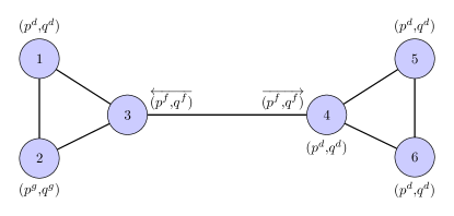
Figure 2: A Simple Network With $|\mathcal{N}|=6$, $|\mathcal{E}|=7$, $|\mathcal{G}|=1$, and $|\mathcal{L}|=4$.

Consider the simplistic power system depicted in Figure 2. There are two areas, $\mathcal{N}^{1}=\{1,2,3\}$ and $\mathcal{N}^{2}=\{4,5,6\}$, which gives $\mathcal{N}^{\leftrightarrow}=\{3,4\}$, $\mathcal{E}^{\leftrightarrow}=\{(3,4),(4,3)\}$. The mapping $\mathcal{O}$ views the setpoints for the generator at bus 2 $(p^{g}_{2},q^{g}_{2})$ as a function of $(p^{d}_{1},q^{d}_{1},p^{d}_{4},q_{4}^{d},p_{5}^{d},q_{5}^{d},p_{6}^{d},q_{6}^{d})$. However, assume that flows $(p_{4,3}^{f},q_{4,3}^{f})$, along with the voltage magnitudes $v_{3},v_{4}$ are fixed and respect constraints ($4$), ($5r$), ($5i$) associated with line $(3,4)$. In that case, the setpoints for the generator at bus 2 can be computed without the knowledge of $(p^{d}_{4},q_{4}^{d},p_{5}^{d},q_{5}^{d},p_{6}^{d},q_{6}^{d})$: the vector $(p_{4,3}^{f},q_{4,3}^{f},v_{3})$ encodes all the information from area 2 needed to compute the generator setpoint. Hence, one may attempt to express $(p^{g}_{2},q^{g}_{2})$ as a function of $(p^{d}_{1},q^{d}_{1},p_{4,3}^{f},q_{4,3}^{f},v_{3})$ which decreases the input size from 8 to 5. The input size decreases by 3 in this example but the size reduction is significantly larger in actual systems.

With this in mind, the mappings in Equation $8$ become

$$\mathcal{O}^{k}:\mathbb{R}^{2|\mathcal{L}^{k}|+|\mathcal{N}^{\to k}|+2|\mathcal{E}^{\to k}|}\to\mathbb{R}^{|\mathcal{N}^{k}\setminus\mathcal{N}^{\to k}|+|\mathcal{E}^{k}|+2|\mathcal{G}^{k}|} 9$$ ()

where the coupling lines, buses of region $k$ are defined as

$$\mathcal{E}^{\to k}=\{(i,j)\in\mathcal{E}^{\leftrightarrow}:i\in\mathcal{N}^{k}\ \vee j\in\mathcal{N}^{k}\}$$

$$\mathcal{N}^{\to k}=\mathcal{N}^{k}\cap\mathcal{N}^{\leftrightarrow}$$

$\mathcal{O}^{k}$ maps the loads in area $k$, the flows to area $k$, and the voltage of the coupling buses to the optimal generator setpoints in the area, i.e., the active and reactive outputs of the regional generators, the phase angle differences of the regional branches, and the voltage setpoints for the non-coupling buses of the region. For large transmission systems, the input/output dimensions of each mapping $\mathcal{O}^{k}$ are significantly smaller that those of $\mathcal{O}$. The learning tasks can proceed in parallel and their complexity is reduced, since each mappings $\mathcal{O}^{k}$ is an order of magnitude smaller in size than $\mathcal{O}$.

Unfortunately, this approach has a key limitation: each mapping $\mathcal{O}^{k}$ can be learned from historical data but cannot be used for prediction since the coupling flows and voltages are not known at prediction time. Indeed, during training, the learning task has access to the coupling values for each instance. However, this is not true at prediction time. The next section shows how to overcome this difficulty.

V Two-Stage Learning of AC-OPF

The fast training method for AC-OPF is a two-stage approach: the first stage is a NN that predicts the flow on the coupling lines and the second stage is a collection of NNs, each of which approximates a mapping $\mathcal{O}^{k}$.

V-A Learning Coupling Voltages & Flows

The goal of the first stage is to learn the mapping

$$\mathcal{O}^{\leftrightarrow}:\mathbb{R}^{2|\mathcal{L}|}\to\mathbb{R}^{|\mathcal{N}^{\leftrightarrow}|+|\mathcal{E}^{\leftrightarrow}|} 13$$ ()

from the loads to the voltages magnitude $\boldsymbol{v}^{0}$ of the coupling buses and the phase angle difference $\boldsymbol{\Delta\theta}^{0}$ of the coupling branches. Although the mapping considers all loads, it can be learned fast (e.g., under 30 minutes) even for large networks, because of the small number of coupling buses and lines. The coupling flows are then computed indirectly via constraints ($5r$) and ($5i$). Let $\mathbb{C}^{\leftrightarrow}$ denote the set of constraints ($2$) for $i\in\mathcal{N}^{\leftrightarrow}$, and ($4$) and ($5r$), ($5i$) for $(i,j)\in\mathcal{E}^{\leftrightarrow}$. The learning task uses a neural network $\mathcal{O}^{\leftrightarrow}[\boldsymbol{w}^{0}]$ parameterized by weights $\boldsymbol{w}^{0}$ and predicts the coupling voltages $(\boldsymbol{\hat{v}}^{0},\boldsymbol{\widehat{\Delta\theta}}^{0})$. The loss function is given by:

$$\mathbb{L}^{\leftrightarrow}(\boldsymbol{\lambda},\boldsymbol{w}^{0})=\mathbb{L}_{0}(\boldsymbol{\hat{v}}^{0},\boldsymbol{\widehat{\Delta\theta}}^{0})+\sum_{c\in\mathbb{C}^{\leftrightarrow}}\lambda_{c}\bar{\nu}_{c}(\boldsymbol{\hat{v}}^{0},\boldsymbol{\widehat{\Delta\theta}}^{0})$$

The training follows equation ($12$) and the resulting optimal weights $(\boldsymbol{w}^{0})^{*}$ lead to the first-stage predictions

$$(\boldsymbol{\hat{v}}^{0},\boldsymbol{\widehat{\Delta\theta}}^{0})=\mathcal{O}^{\leftrightarrow}[(\boldsymbol{w}^{0})^{*}](\boldsymbol{p^{d}},\boldsymbol{q^{d}})$$

and the resulting first-stage coupling flow predictions $(\boldsymbol{\hat{p}^{f}})^{0},(\boldsymbol{\hat{q}^{f}})^{0}$. The first stage is summarized in Algorithm 1.

$\lambda_{c}\leftarrow 0,\forall c\in\mathbb{C}^{\leftrightarrow}$

for $i=1,2,...,epochs_{\lambda}$ do

       for $j=1,2,...,epochs_{w}$ do

             $(\boldsymbol{\hat{v}}^{0},\boldsymbol{\widehat{\Delta\theta}}^{0})\leftarrow\mathcal{O}^{\leftrightarrow}[\boldsymbol{w}^{0}](\boldsymbol{p^{d}},\boldsymbol{q^{d}})$

             $\mathbb{L}^{\leftrightarrow}(\boldsymbol{\lambda},\boldsymbol{w}^{0})\leftarrow\mathbb{L}_{0}(\boldsymbol{\hat{v}}^{0},\boldsymbol{\widehat{\Delta\theta}}^{0})+\sum_{c\in\mathbb{C}^{\leftrightarrow}}\lambda_{c}\bar{\nu}_{c}(\boldsymbol{\hat{v}}^{0},\boldsymbol{\widehat{\Delta\theta}}^{0})$

             $\boldsymbol{w}^{0}\leftarrow\boldsymbol{w}^{0}-\alpha\nabla_{\boldsymbol{w}^{0}}(\mathbb{L}^{\leftrightarrow}(\boldsymbol{\lambda},\boldsymbol{w}^{0}))$

       end for

      $\lambda_{c}\leftarrow\lambda_{c}+\rho\bar{\nu}_{c},\quad\forall c\in\mathbb{C}^{\leftrightarrow}$

end for

Result: Weights $(\boldsymbol{w}^{0})^{*}$

Algorithm 1 The First-Stage Coupling Training.

V-B Training of Regional Systems

The training of the regional systems uses the first-stage predictions for the coupling flows and voltages. Note however that it could use the ground truth present in the instance data, but experimental results have shown that this degrades the overall prediction accuracy. The decoupling is illustrated in Figure 3, where the voltages of the coupling buses $3$ and $4$ and the incoming/outgoing flows for each region are fixed to the first-stage predictions.

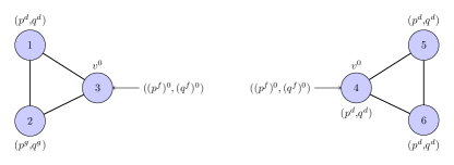
Figure 3: Illustration of the Decomposition.

To learn mappings $\mathcal{O}^{k}\ (k\in[K])$, let $\mathbb{C}^{k}$ denote the set of constraints associated with region $k$, i.e., constraint ($2$) for buses $i\in\mathcal{N}^{k}\setminus\mathcal{N}^{\to k}$, constraints ($3r$), ($3i$), ($6r$), and ($6i$) for buses $i\in\mathcal{N}^{k}$, and constraints ($4$), ($5r$), ($5i$) for branches $(i,j)\in\mathcal{E}^{k}$. In particular, the power balance constraint ($6r$), ($6i$) for region $k$ becomes

$$p_{i}^{g}-(p_{i}^{d}-\sum_{(i,j)\in\mathcal{E}^{\to k}}(\hat{p}_{ij}^{f})^{0})=\sum_{(i,j)\in\mathcal{E}^{k}}p_{ij}^{f} i\in\mathcal{N}^{k}$$

$$q_{i}^{g}-(q_{i}^{d}-\sum_{(i,j)\in\mathcal{E}^{\to k}}(\hat{q}_{ij}^{f})^{0})=\sum_{(i,j)\in\mathcal{E}^{k}}q_{ij}^{f} i\in\mathcal{N}^{k}$$

The learning task uses a collection $\{\mathcal{O}^{k}[\boldsymbol{w}^{k}]\}_{k\in[K]}$ of NNs and the loss function for each regional net is given by

$$\mathbb{L}^{k}(\boldsymbol{\lambda},\boldsymbol{w}^{k})=\mathbb{L}_{0}(\boldsymbol{\hat{v}}^{k},\boldsymbol{\widehat{\Delta\theta}}^{k},(\boldsymbol{\hat{p}^{g}})^{k},(\boldsymbol{\hat{q}^{g}})^{k})+$$

$$\sum_{c\in\mathbb{C}^{k}}\lambda_{c}\bar{\nu}_{c}(\boldsymbol{\hat{v}}^{k},\boldsymbol{\widehat{\Delta\theta}}^{k},(\boldsymbol{\hat{p}^{g}})^{k},(\boldsymbol{\hat{q}^{g}})^{k},\boldsymbol{\hat{v}}^{0,k},(\boldsymbol{\hat{p}^{f}})^{0,k},(\boldsymbol{\hat{q}^{f}})^{0,k})$$

where $\boldsymbol{\hat{v}}^{0,k}$ is the first-stage prediction for the voltage magnitude of the coupling buses of region $k$ and $(\boldsymbol{\hat{p}^{f}})^{0,k},(\boldsymbol{\hat{q}^{f}})^{0,k}$ the first-stage predictions for the incoming/outgoing flows of region $k$. The training, summarized in Algorithm 2, is performed using the approach in equation ($12$) and each region can be trained in parallel. Line 2 predicts the voltage setpoints for the coupling buses and the phase angle differences of the coupling lines. Line 3 computes the predicted coupling flows from these predictions. Line 6 computes the predictions for region $k$ given the current NN parameters and constraint weights. Line 8 performs the back-propagation to update the weights and line 10 updates the constraint weights.

$\lambda_{c}\leftarrow 0,\forall c\in\mathbb{C}^{k}$

$(\boldsymbol{\hat{v}}^{0},\boldsymbol{\widehat{\Delta\theta}}^{0})\leftarrow\mathcal{O}^{\leftrightarrow}[(\boldsymbol{w}^{0})^{*}](\boldsymbol{p^{d}},\boldsymbol{q^{d}})$

Compute $(\boldsymbol{\hat{p}^{f}})^{0,k},(\boldsymbol{\hat{q}^{f}})^{0,k}$ via ($5r$), ($5i$)

for $i=1,2,...,epochs_{\lambda}$ do

       for $j=1,2,...,epochs_{w}$ do

             $(\boldsymbol{\hat{v}}^{k},\boldsymbol{\widehat{\Delta\theta}}^{k},(\boldsymbol{\hat{p}^{g}})^{k},(\boldsymbol{\hat{q}^{g}})^{k})\leftarrow\mathcal{O}^{k}[\boldsymbol{w}^{k}]((\boldsymbol{p^{d}})^{k},(\boldsymbol{q^{d}})^{k},\boldsymbol{\hat{v}}^{0,k},(\boldsymbol{\hat{p}^{f}})^{0,k},(\boldsymbol{\hat{q}^{f}})^{0,k})$

             $\mathbb{L}^{k}(\boldsymbol{\lambda},\boldsymbol{w}^{k})\leftarrow\mathbb{L}_{0}(\boldsymbol{\hat{v}}^{k},\boldsymbol{\widehat{\Delta\theta}}^{k},(\boldsymbol{\hat{p}^{g}})^{k},(\boldsymbol{\hat{q}^{g}})^{k})+\sum_{c\in\mathbb{C}^{k}}\lambda_{c}\bar{\nu}_{c}((\boldsymbol{\hat{v}},\boldsymbol{\widehat{\Delta\theta}},\boldsymbol{\hat{p}^{g}},\boldsymbol{\hat{q}^{g}},\boldsymbol{\hat{v}}^{0},(\boldsymbol{\hat{p}^{f}})^{0},(\boldsymbol{\hat{q}^{f}})^{0})^{k})$

             $\boldsymbol{w}^{k}\leftarrow\boldsymbol{w}^{k}-\alpha\nabla_{\boldsymbol{w}^{k}}(\mathbb{L}^{k}(\boldsymbol{\lambda},\boldsymbol{w}^{k}))$

       end for

      $\lambda_{c}\leftarrow\lambda_{c}+\rho\bar{\nu}_{c},\quad\forall c\in\mathbb{C}^{k}$

end for

Result: Weights $(\boldsymbol{w}^{k})^{*}$

Algorithm 2 The Second-Stage Training (Region $k$).

VI Experimental Results

VI-A Experimental Setting

The datasets were generated by solving AC-OPF problems with the nonlinear solver IPOPT [28] using 2.5 GHz-i7 Intel Cores and 16GB of RAM. In total, $10^{4}$ load profiles, which correspond to feasible AC-OPF problems, were generated for each test case. $80\%$ of these instances were used for training and the remaining $20\%$ for testing. The learning models were implemented using PyTorch [29] and trained using NVidia Tesla V100 GPUs with 16GB of memory. The training of each network utilizes mini-batches of size 120 and the learning rate $\alpha$ was set to be decreasing from $10^{-3}$ to $10^{-6}$, while $\rho$ was set to $10^{-3}$.

The first-stage NN consists of two subnetworks with sizes $2|\mathcal{L}|\times|\mathcal{N}^{\leftrightarrow}|\times|\mathcal{N}^{\leftrightarrow}|$ and $2|\mathcal{L}|\times|\mathcal{E}^{\leftrightarrow}|\times|\mathcal{E}^{\leftrightarrow}|$ for the voltage magnitudes and phase angle differences respectively. For each region, each NN topology consists of 4 subnetworks, one for each predicted variable. The subnetworks have one hidden layer of size $2|\mathcal{L}^{k}|\times 3|\mathcal{L}^{k}|\times|\mathcal{G}^{k}|$. The subnetworks used to approximate the original mapping (equation ($7$)) are similar in structure and have size $2|\mathcal{L}|\times 3|\mathcal{L}|\times|\mathcal{G}|$.

VI-B Load Profiles

TABLE I: The Power System Networks with Regional Information

Benchmark	$|\mathcal{N}|$	$|\mathcal{E}|$	$|\mathcal{L}|$	$|\mathcal{G}|$	$|\mathcal{N}^{k}|_{k=1}^{K}$	$|\mathcal{E}^{\leftrightarrow}|$
France_EHV	1737	2350	1731	290	[338, 280, 233, 179, 143, 126, 124, 72, 67, 64, 57, 54]	148
France_Lyon	3411	4499	3273	771	[1158, 357, 294, 288, 264, 255, 231, 197, 184, 67, 62, 54]	219
France	6705	8962	6262	1708	[1156, 796, 748, 746, 627, 517, 497, 395, 325, 322, 298, 278]	326

The power systems used as test cases (Table I) are parts of the actual French Transmission System. France is the French transmission system, France_EHV is the very high-voltage French system, and France_LYON is France_EHV with a detailed representation of the Lyon region. The French system is organized in 12 geographical regions. The dataset is generated by taking into account this geographical information. A load $l$ in region $k$ with nominal value $(p^{d},q^{d})^{0}$ is generated with the formula

$$(p^{d},q^{d})=(\alpha+\beta^{k}+\gamma^{l})((p^{d})^{0},(q^{d})^{0})$$

where the following coefficients are randomly drawn from the folowing distributions

$$\alpha\sim\text{Uniform}[0.875,0.975]$$

$$\beta^{k}\sim\text{Uniform}[-0.025,0.025],\quad\forall k\in[K]$$

$$\gamma^{l}\sim\text{Uniform}[-0.0025,0.0025],\quad\forall l\in\mathcal{L}$$

The term $\alpha$ captures the system-wide load level, while $\beta^{k}$ is associated with differences in the loads between regions (e.g., due to potentially different weather conditions). The difference in coefficients may be up to $5\%$ for two different regions. Finally, $\gamma^{l}$ is the uncorrelated noise added to each individual load with a range of $0.5\%$ of its nominal value.

The resulting dataset captures realistic load profiles: the uniform load perturbation, the load level differences between the regions, and the fixed active/reactive power ratio represent the typical behavior for aggregated demand in a large-scale topology spanning several geographic regions. Randomly perturbing each individual load in an uncorrelated fashion would produce unrealistic load profiles: they would lead to an unnecessarily challenging learning task that would need to capture an exponential number of unrealistic behaviors of the power system. To highlight this point, Figure 4 depicts the actual consumption for three French regions over a 12 hour interval. Observe the strong correlation of the demand between the three regions. However, the correlation is not perfect and the ratios between the regional loads vary by small factors. The term $\beta_{k}$ is used to account for this behavior. The resulting load profiles range from 0.85 of the nominal to the nominal load. This $15\%$ difference is typical over a 12-hour interval as shown in Figure 4.

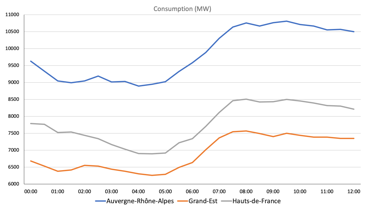
Figure 4: Consumption for Three Regions in the French System over a 12-hour Interval.

VI-C First-stage Predictions

This section presents the prediction errors of the first stage. The training time was limited to 30 minutes. Table II contains aggregate results for the active and reactive powers of the coupling branches, as well the voltage magnitudes, for all three test cases. The results are an average over all instances and coupling branches. The average error is close to $1\ \mbox{MW}$ for the largest two test cases: France and France_Lyon. Meanwhile, the $95$-Quantile indicates that $95$% of the predictions result in an error less that $5\ \mbox{MW}$. In the smaller France_EHV, the errors are slightly higher reaching $3.5\ \mbox{MW}$ on average. Given that the nominal load of the France system is $50,000\ \mbox{MW}$) and the nominal flow values for most coupling branches are greater than $100\ \mbox{MW}$ and go up to $1,000\ \mbox{MW}$), these results indicate that the prediction errors are small in percentage for all test cases. Table II also shows that the voltage magnitudes are predicted very accurately. Figure 5 contains detailed results on the active part of the flows of the coupling branches for the France test case, showing consistent results across all tested instances. The $95\%$ quantile graph indicates that the prediction errors exceed $5\ \mbox{MW}$ only for a very small percentage of the test cases and branches.

	$\hat{p}^{f}$ (MW)		$v$ (P.U)
Benchmark	Avg	$95\%$ Quantile	Avg	$95\%$ Quantile
France_EHV	3.43	11.91	25 $\cdot 10^{-5}$	$76\cdot 10^{-5}$
France_Lyon	1.25	4.89	27 $\cdot 10^{-5}$	$82\cdot 10^{-5}$
France	0.99	4.11	50 $\cdot 10^{-5}$	$153\cdot 10^{-5}$

TABLE II: Absolute Errors for the Voltage Magnitude at the Coupling Buses and the Active Power Flow of the Coupling Branches.

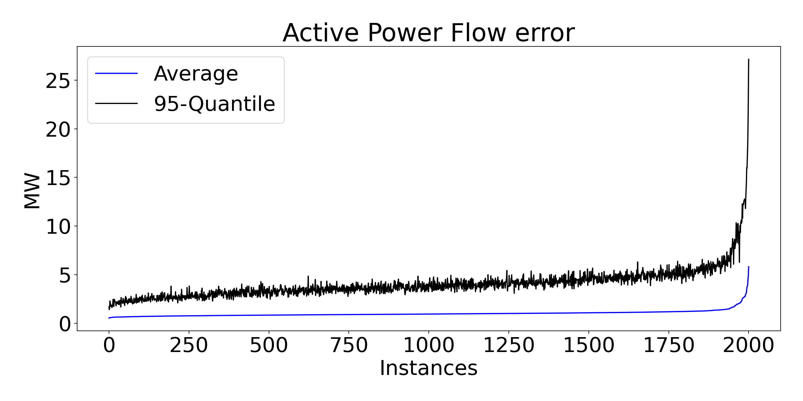
Figure 5: Prediction Errors (Average and 95$\%$ Quantile) over all Testing Instances for the Active Flow of the Coupling Branches for Testcase France. The Instances are Sorted in Increasing Order of Average Error.

VI-D Performance of the Learning Models

This section compares the model $\mathbb{O}$ that directly approximates the mapping $\mathcal{O}$ (Equation $7$) with the proposed two-stage approach $\mathbb{D}$. The results show that, with a time limit of 90 minutes, $\mathbb{D}$ outperforms $\mathbb{O}$ and is more scalable. In model $\mathbb{D}$, 30 minutes is allocated to the first stage, and 60 minutes to the second stage. The comparison is performed on the smaller systems, France_EHV and LYON, which represents the high-voltage French system and the high-voltage French with a detailed representation of the Lyon region. Experimental results on the full French system are only given for model $\mathbb{D}$, since the original model exceeds the capacity of the GPU memory. The comparison consists of three parts. The first part reports the accuracy for variables $(\hat{\boldsymbol{v}},\hat{\boldsymbol{p}}^{g})$ (that are directly predicted) and the indirectly predicted $\hat{\boldsymbol{p}}^{f}$. The second part considers constraint violations. The third part discusses how the predictions can be used to seed an optimization model that restores feasibility.

VI-D1 Prediction Accuracy

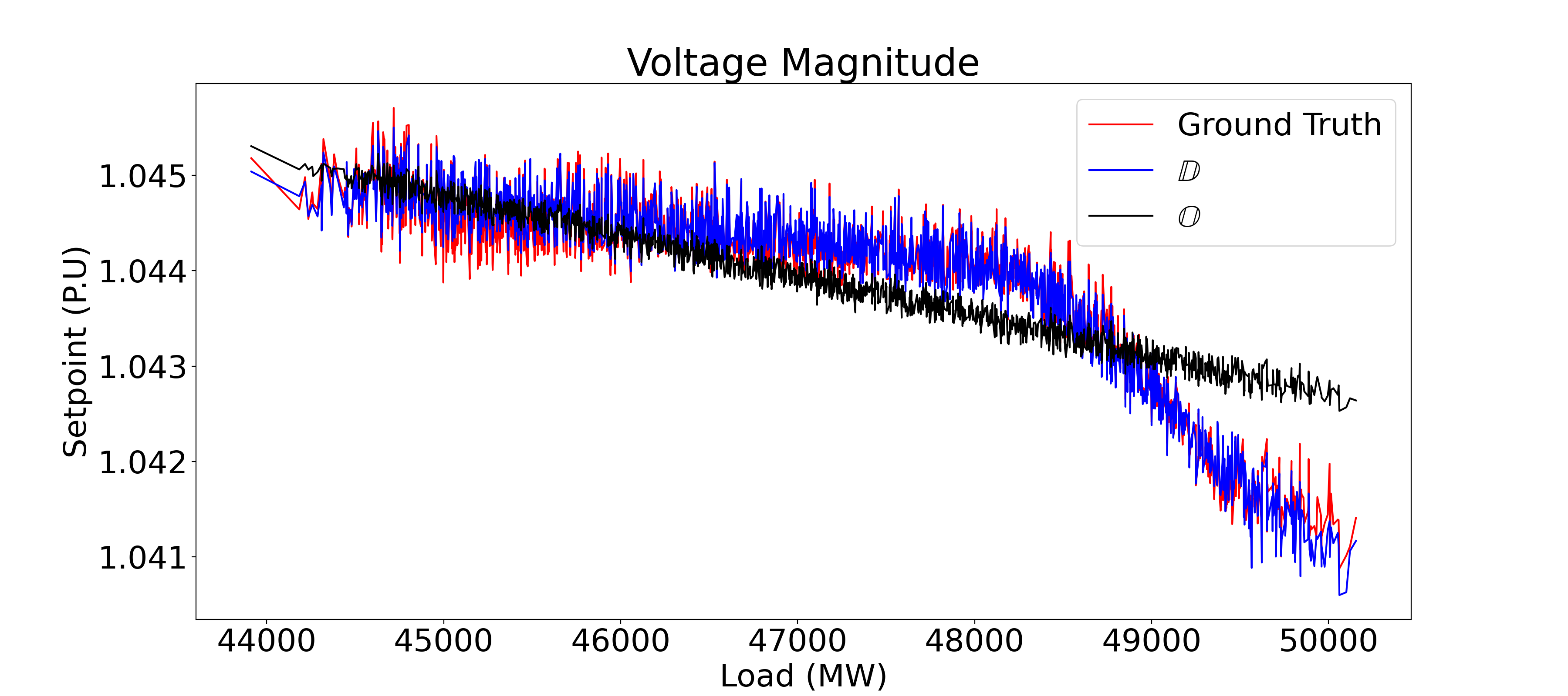
(a) Voltage Magnitude

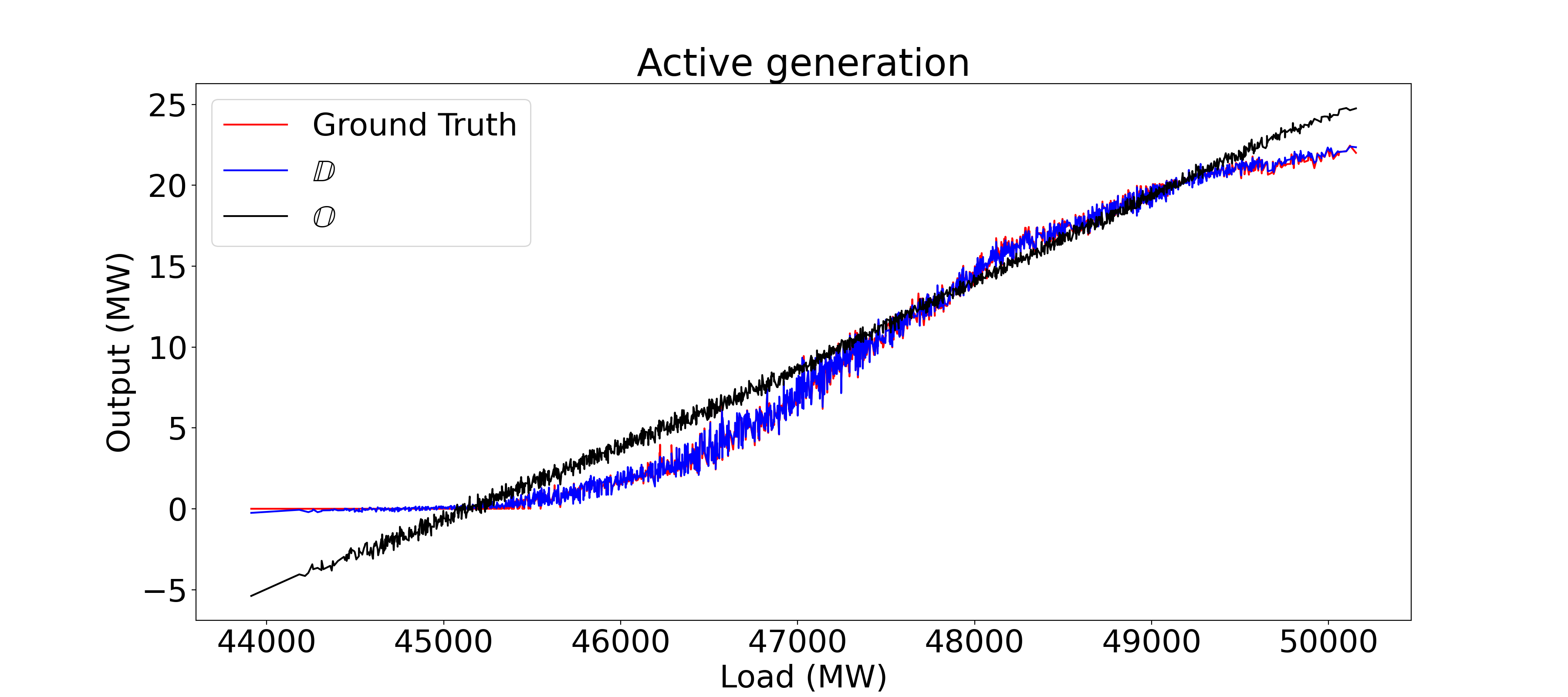
(b) Active power

Figure 6: Convergence of $\mathbb{O}$ and $\mathbb{D}$ Illustrated for a Bus and Generator.

(a) Voltage Magnitude

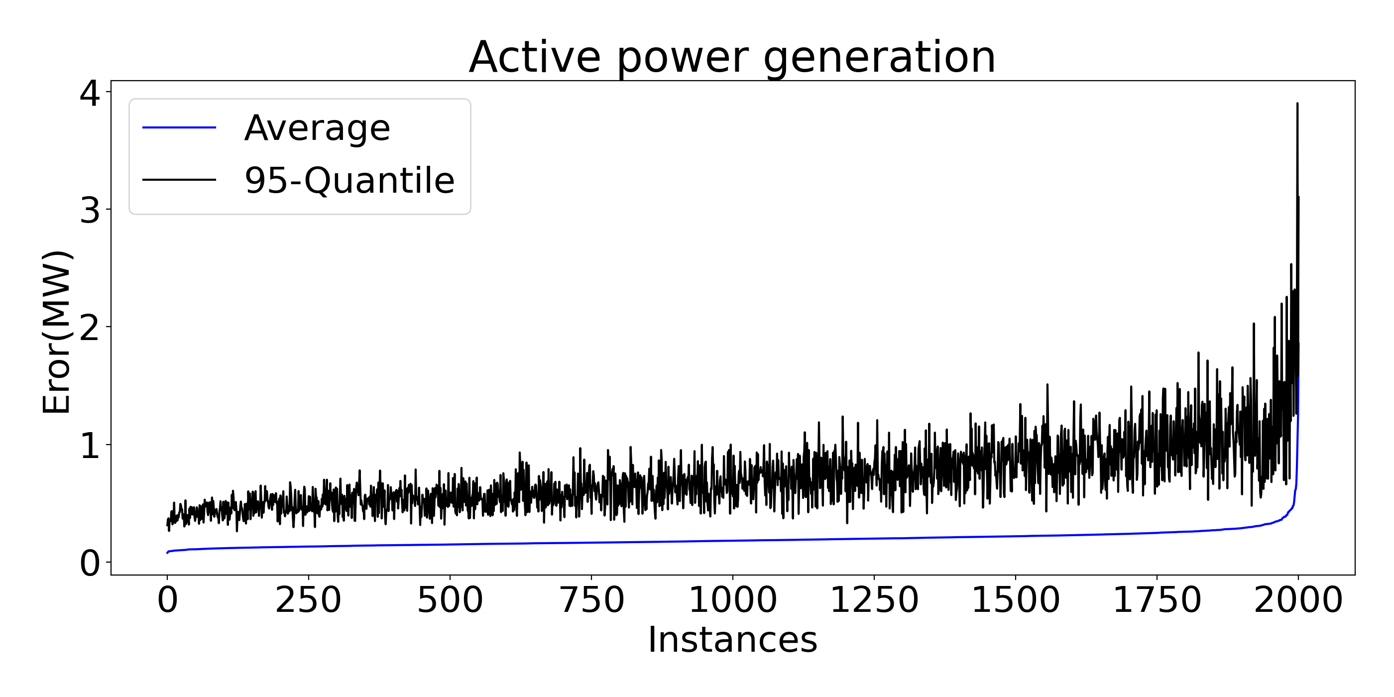
(b) Active power

Figure 7: Prediction Errors for the France System using Model $\mathbb{D}$.

Figure 6 illustrate the convergence of the two models for the predicted variables $\hat{\boldsymbol{v}},\hat{\boldsymbol{p}}^{g}$ for a specific bus and generator from the France_LYON test case. The x-axis corresponds to test instances sorted by increasing system load. There is significant volatility in the ground truth values since instances that are close in the x-axis do not necessarily correspond to similar load vectors. Indeed, a similar overall system load may exhibit significant regional load differences. The results demonstrate that, for voltage magnitudes, model $\mathbb{O}$ has significant errors. The same hold for active power. In constrast, model $\mathbb{D}$ closely follows the ground truth for voltage magnitudes and exhibits minor errors for active power predictions. The difference between the two models is quite striking.

Tables III, IV, and V summarize the tprediction errors over all testcases, buses, generators, and lines, as well the $95\%$ Quantile. The tables omit all power results for generators that are either off for all instances (due to potentially high cost) or constantly producing at their respective upper bounds (due to low cost). For voltage magnitudes, model $\mathbb{D}$ divides the error in half compared to model $\mathbb{O}$. This difference is significant for the prediction of the power flows and constraint violations. Figure 7 demonstrates that model $\mathbb{D}$ scales to the size of the France system and continues to produce highly accurate predictions. For active power, model delivers predictions whose errors are an order of magnitude smaller than those of model $\mathbb{O}$. The average errors are below $1\ \mbox{MW}$, which is small compared to the total system load ($\sim$ $50,000\ \mbox{MW}$). Again, Figure 7 demonstrates that model $\mathbb{D}$ nicely scales to the France system. The benefits of model $\mathbb{D}$ are abundantly clear for the power flow predictions $\hat{p}^{f}$, which are indirectly predicted as a function of the predictions $\hat{v}$ and $\hat{\theta}$. For France_LYON, the second largest test case, model $\mathbb{O}$ results in large errors (up to $50\ \mbox{MW}$). In contrast, model $\mathbb{D}$ results in minor errors, with $95$% of the predictions having an error of at most $1.04\ \mbox{MW}$ in the largest benchmark. Compared to the overall system scale, these errors are small in percentage. Note that accurate predictions for power flows are critical for low violation degrees of the AC-OPF constraints.

	Model $\mathbb{O}$		Model $\mathbb{D}$
Benchmark	Avg	$95\%$ Quantile	Avg	$95\%$ Quantile
France_EHV	$39\cdot 10^{-5}$	$125\cdot 10^{-5}$	$22\cdot 10^{-5}$	$61\cdot 10^{-5}$
France_Lyon	$45\cdot 10^{-5}$	$127\cdot 10^{-5}$	$22\cdot 10^{-5}$	$78\cdot 10^{-5}$
France	-	-	$25\cdot 10^{-5}$	$84\cdot 10^{-5}$

TABLE III: Prediction Errors (P.U.) for Voltage Magnitudes ($\hat{v}$).

	Model $\mathbb{O}$		Model $\mathbb{D}$
Benchmark	Avg	$95\%$ Quantile	Avg	$95\%$ Quantile
France_EHV	$8.41$	$50.82$	$0.84$	$3.27$
France_Lyon	$8.93$	$47.54$	$0.30$	$0.94$
France	-	-	$0.19$	$0.70$

TABLE IV: Prediction Errors (MW) for Active Power ($\hat{p}^{g}$).

	Model $\mathbb{O}$		Model $\mathbb{D}$
Benchmark	Avg	$95\%$ Quantile	Avg	$95\%$ Quantile
France_EHV	$4.53$	$16.88$	$2.01$	$4.20$
France_Lyon	$8.43$	$32.20$	$0.82$	$1.91$
France	-	-	$0.45$	$1.04$

TABLE V: Prediction Errors (MW) for Active Power Flow ($\hat{p}^{f}$).

	Model $\mathbb{O}$		Model $\mathbb{D}$
Benchmark	$v$	$p^{g}$	$v$	$p^{g}$
France_EHV	$99.90$	$98.46$	$99.74$	$99.94$
France_Lyon	$99.72$	$99.24$	$99.91$	$99.99$
France	-	-	$99.97$	$99.99$

TABLE VI: Percentage of AC-OPF bound Constraints with Violations under $1\ \mbox{MW}$ (for $\hat{p}^{g}$) and under $10^{-4}$ P.U. (for $\hat{v}$)

	Model $\mathbb{O}$		Model $\mathbb{D}$
Benchmark	Avg	$95\%$ Quantile	Avg	$95\%$ Quantile
France_EHV	$4.49$	$16.20$	$4.82$	$9.77$
France_Lyon	$18.65$	$100.36$	$1.91$	$4.67$
France	-	-	$1.05$	$2.39$

TABLE VII: Violation for the Active Power Balance Constraint (MW).

VI-D2 Feasibility

Table VI reports the constraint violations for the bounds on active power and voltage magnitude (constraints ($2$), ($3r$)). Model $\mathbb{D}$ has minor violations for $99.9\%$ of these constraints. Table VII report the violations of the active flow conservation constraints. Again, model $\mathbb{D}$ has an average $1.05\ \mbox{MW}$ violations in the France test case, which is insignificant compared to the scale of the system.

VI-D3 Load-Flow Analysis

This section shows how model $\mathbb{D}$ can also be used for applications that require a high-quality feasible solution to AC-OPF. It presents an optimization model, called a Load Flow (L-F) model, for finding the feasible AC-OPF solution that is closest to the prediction of model $\mathbb{D}$, i.e.,

$$\min \quad\lvert\lvert\boldsymbol{p^{g}}-\boldsymbol{\hat{p}^{g}}\rvert\rvert_{2}^{2}+\lvert\lvert\boldsymbol{v}-\boldsymbol{\hat{v}}\rvert\rvert_{2}^{2} 14$$ ()

s.t $$\quad\text{(\ref{con:2}) - (\ref{con:6b}}).$$

	Model $\mathbb{O}$		Model $\mathbb{D}$
Benchmark	Avg	Max	Avg	Max
France_EHV	$0.036$	$0.193$	$0.026$	$0.119$
France_Lyon	$0.281$	$0.987$	$0.016$	$0.071$
France	-	-	$0.012$	$0.030$

TABLE VIII: Objective Value Increase of the Load-Flow Solution (in $\%$) Compared to AC-OPF Objective.

Table VIII reports the objective increase in the load flow solution with models $\mathbb{D}$ and $\mathbb{O}$ compared to the AC-OPF solution, i.e.,

$$\frac{1}{N_{test}}\sum_{i=1}^{N_{test}}\lvert 1-\frac{cost_{LF}}{cost_{AC}}\rvert\times 100\%$$

where $cost_{LF}$ denotes the load flow cost and $cost_{AC}$ denotes the AC-OPF cost. The load flow based on model $\mathbb{D}$ is within $<0.03\%$ on average of the AC-OPF solution and one magnitude smaller compared to the solutions provided by $\mathbb{O}$ on the France_Lyon testcase.

	L-F $\mathbb{O}$		L-F $\mathbb{D}$		AC-OPF
Benchmark	Avg	Max	Avg	Max	Avg	Max
France_EHV	$7.14$	$11.72$	$6.70$	$10.83$	$7.10$	$10.51$
France_Lyon	$38.21$	$186.71$	$20.08$	$26.75$	$75.20$	$215.47$
France	-	-	$65.21$	$130.67$	$164.07$	$315.97$

TABLE IX: Comparison of the Load Flow and AC-OPF Computation Times (in seconds).

In terms of computational efficiency, model $\mathbb{D}$ delivers a prediction in a few milliseconds, which makes it sufficient to compare the optimization results only. Table IX compares the execution times of the load flow and the AC-OPF optimizations. The results demonstrate that the load flow optimization is significantly faster compared to the AC-OPF optimization on the largest two benchmarks. This indicates that a combination of machine learning and optimization is beneficial when a near-optimal AC-feasible solution to the OPF is desired.

VII Conclusion

This paper considered the design of a fast and scalable training for a machine-learning model that predicts AC-OPF solutions. It was motivated by the facts that (1) topology optimization and the stochasticity induced in renewable energy may lead to fundamentally different AC-OPF instances; and (2) existing machine-learning algorithms for AC-OPF require significant training time of and do not scale to the size of real transmission systems. The paper proposed a novel 2-stage approach that exploits a spatial network decomposition. The power network is viewed as a set of regions, the first stage learns to predict the flows and voltages on the buses and lines that are coupling the regions, and the second stage trains, in parallel, the machine-learning models for each region. Experimental results on the French transmission system (up to 6,700 buses and 9,000 lines) demonstrate the potential of the approach. Within a training time of 90 minutes, the approach predicts AC-OPF solutions with very high fidelity (e.g., an average error of 1 MW for an overall load of 50 GW) and minor constraint violations, producing significant improvements over the state-of-the-art. The results also show that the predictions can be used to seed a load flow optimization that returns a feasible solution within $0.03\%$ of the AC-OPF objective, while reducing the running times by a factor close to 3. Future work will focus on generalizing the approach to security-constrained OPF, by studying how to merge the algorithm proposed in [3] to the AC setting and the proposed 2-stage approach.

References

- [1] K. Lehmann, A. Grastien, and P. Van Hentenryck, “Ac-feasibility on tree networks is np-hard,” IEEE Transactions on Power Systems, vol. 31, no. 1, pp. 798–801, 2016.
- [2] A. Monticelli, M. Pereira, and S. Granville, “Security-constrained optimal power flow with post-contingency corrective rescheduling,” IEEE Transactions on Power Systems, vol. 2, no. 1, pp. 175–180, 1987.
- [3] A. Velloso, P. V. Hentenryck, and E. S. Johnson, “An exact and scalable problem decomposition for security-constrained optimal power flow,” 2019.
- [4] J. Wang, M. Shahidehpour, and Z. Li, “Security-constrained unit commitment with volatile wind power generation,” IEEE Transactions on Power Systems, vol. 23, no. 3, pp. 1319–1327, 2008.
- [5] E. B. Fisher, R. P. O’Neill, and M. C. Ferris, “Optimal transmission switching,” IEEE Transactions on Power Systems, vol. 23, no. 3, pp. 1346–1355, Aug 2008.
- [6] M. E. Baran and F. F. Wu, “Optimal capacitor placement on radial distribution systems,” IEEE Transactions on Power Delivery, vol. 4, no. 1, pp. 725–734, Jan 1989.
- [7] Niharika, S. Verma, and V. Mukherjee, “Transmission expansion planning: A review,” in International Conference on Energy Efficient Technologies for Sustainability, April 2016, pp. 350–355.
- [8] M. Chatzos, F. Fioretto, T. W. K. Mak, and P. V. Hentenryck, “High-fidelity machine learning approximations of large-scale optimal power flow,” ArXiv 2006.16356 [eess.SP], 2020.
- [9] F. Fioretto, T. W. Mak, and P. Van Hentenryck, “Predicting AC optimal power flows: Combining deep learning and lagrangian dual methods,” in Proceedings of the AAAI Conference on Artificial Intelligence (AAAI), 2020, pp. 630–637.
- [10] L. Duchesne, E. Karangelos, and L. Wehenkel, “Recent developments in machine learning for energy systems reliability management,” Proc. IEEE, vol. 108, no. 9, pp. 1656–1676, 2020. [Online]. Available: https://doi.org/10.1109/JPROC.2020.2988715
- [11] F. Hasan, A. Kargarian, and A. Mohammadi, “A survey on applications of machine learning for optimal power flow,” in 2020 IEEE Texas Power and Energy Conference (TPEC), 2020, pp. 1–6.
- [12] S. Misra, L. Roald, and Y. Ng, “Learning for constrained optimization: Identifying optimal active constraint sets,” 2019.
- [13] A. S. Xavier, F. Qiu, and S. Ahmed, “Learning to solve large-scale security-constrained unit commitment problems,” 2019.
- [14] D. Deka and S. Misra, “Learning for DC-OPF: Classifying active sets using neural nets,” in 2019 IEEE Milan PowerTech, June 2019.
- [15] F. Hasan, A. Kargarian, and J. Mohammadi, “Hybrid learning aided inactive constraints filtering algorithm to enhance ac opf solution time,” 2020.
- [16] A. Robson, M. Jamei, C. Ududec, and L. Mones, “Learning an optimally reduced formulation of opf through meta-optimization,” 2020.
- [17] K. Baker, “A learning-boosted quasi-newton method for ac optimal power flow,” 2020.
- [18] ——, “Learning warm-start points for ac optimal power flow,” 2019.
- [19] L. Chen and J. E. Tate, “Hot-starting the ac power flow with convolutional neural networks,” 2020.
- [20] X. Pan, T. Zhao, and M. Chen, “Deepopf: Deep neural network for dc optimal power flow,” in 2019 IEEE International Conference on Communications, Control, and Computing Technologies for Smart Grids (SmartGridComm), 2019, pp. 1–6.
- [21] X. Pan, M. Chen, T. Zhao, and S. H. Low, “Deepopf: A feasibility-optimized deep neural network approach for ac optimal power flow problems,” 2020.
- [22] A. Zamzam and K. Baker, “Learning optimal solutions for extremely fast AC optimal power flow,” CoRR, vol. abs/1910.01213, 2019. [Online]. Available: http://arxiv.org/abs/1910.01213
- [23] T. W. K. Mak, F. Fioretto, and P. VanHentenryck, “Load embeddings for scalable ac-opf learning,” ArXiv 2101.03973 [eess.SY], 2021.
- [24] A. Venzke and S. Chatzivasileiadis, “Verification of neural network behaviour: Formal guarantees for power system applications,” I E E E Transactions on Smart Grid, 2020.
- [25] A. Venzke, G. Qu, S. Low, and S. Chatzivasileiadis, “Learning optimal power flow: Worst-case guarantees for neural networks,” 2020.
- [26] X. Pan, T. Zhao, M. Chen, and S. Zhang, “Deepopf: A deep neural network approach for security-constrained dc optimal power flow,” 2020.
- [27] A. Velloso and P. V. Hentenryck, “Combining deep learning and optimization for security-constrained optimal power flow,” IEEE Transactions on Power Systems, to appear (2021).
- [28] A. Wächter and L. T. Biegler, “On the implementation of an interior-point filter line-search algorithm for large-scale nonlinear programming,” Mathematical Programming, vol. 106, no. 1, pp. 25–57, 2006.
- [29] A. Paszke, S. Gross, S. Chintala, G. Chanan, E. Yang, Z. DeVito, Z. Lin, A. Desmaison, L. Antiga, and A. Lerer, “Automatic differentiation in pytorch,” 2017.