UFIFT-QG-20-06

Inflaton Effective Potential from Photons for General $\epsilon$

S. Katuwal^1∗, S. P. Miao^2⋆ and R. P. Woodard^1†

¹ Department of Physics, University of Florida,
Gainesville, FL 32611, UNITED STATES

² Department of Physics, National Cheng Kung University,
No. 1 University Road, Tainan City 70101, TAIWAN

ABSTRACT

We accurately approximate the contribution that photons make to the effective potential of a charged inflaton for inflationary geometries with an arbitrary first slow roll parameter $\epsilon$. We find a small, nonlocal contribution and a numerically larger, local part. The local part involves first and second derivatives of $\epsilon$, coming exclusively from the constrained part of the electromagnetic field which carries the long range interaction. This causes the effective potential induced by electromagnetism to respond more strongly to geometrical evolution than for either scalars, which have no derivatives, or spin one half particles, which have only one derivative. For $\epsilon=0$ our final result agrees with that of Allen [1] on de Sitter background, while the flat space limit agrees with the classic result of Coleman and Weinberg [2].

PACS numbers: 04.50.Kd, 95.35.+d, 98.62.-g

^∗ e-mail: sanjib.katuwal@ufl.edu

^⋆ email: spmiao5@mail.ncku.edu.tw

^† e-mail: woodard@phys.ufl.edu

1 Introduction

No one knows what caused primordial inflation but the data [3] are consistent with a minimally coupled, complex scalar inflaton $\varphi$,

$$\mathcal{L}=-\partial_{\mu}\varphi\partial_{\nu}\varphi^{*}g^{\mu\nu}\sqrt{-g}-V(\varphi\varphi^{*})\sqrt{-g}\;.$$ (1)

If the inflaton couples only to gravity the loop corrections to its effective potential come only from quantum gravity and are suppressed by powers of the loop-counting parameter $GH^{2}\mathrel{\raise 1.29167pt\hbox{$<$\kern-7.5pt\lower 4.30554pt\hbox{$\sim$}}}10^{-10}$, where $G$ is Newton’s constant and $H$ is the Hubble parameter during inflation. In that case the classical evolution suffers little disturbance but reheating is very slow.

Efficient reheating requires coupling the inflaton to normal matter such as electromagnetism with a non-infinitesimal charge $q$,

$$\mathcal{L}=-\Bigl{(}\partial_{\mu}-iqA_{\mu}\Bigr{)}\varphi\Bigl{(}\partial_{\nu}+iqA_{\nu}\Bigr{)}\varphi^{*}g^{\mu\nu}\sqrt{-g}$$ (2)

$$\hskip 142.26378pt-V(\varphi\varphi^{*})\sqrt{-g}-\frac{1}{4}F_{\mu\nu}F_{\rho\sigma}g^{\mu\rho}g^{\nu\sigma}\sqrt{-g}\;.\qquad$$

But the price of efficient reheating is significant one loop corrections to the inflaton effective potential [4]. For large fields these corrections approach the Coleman-Weinberg form of flat space $\Delta V\longrightarrow\frac{3}{16\pi^{2}}(q^{2}\varphi\varphi^{*})^{2}\ln(q^{2}\varphi\varphi^{*}/s^{2})$, where $s$ is the renormalization scale [2]. However, cosmological Coleman-Weinberg potentials generally depend in a complicated way on the geometry of inflation [5],

$$ds^{2}=a^{2}\Bigl{[}-d\eta^{2}+d\vec{x}\!\cdot\!d\vec{x}\Bigr{]}\qquad\Longrightarrow\qquad H\equiv\frac{\partial_{0}a}{a^{2}}\;\;,\;\;\epsilon(t)\equiv-\frac{\partial_{0}H}{aH^{2}}\;.$$ (3)

For the special case of de Sitter (with constant $H$ and $\epsilon=0$) the result takes the form [1, 6, 7],

$$\Delta V\Bigl{|}_{\epsilon=0}=\frac{3H^{4}}{16\pi^{2}}\Biggl{\{}b\Bigl{(}\frac{q^{2}\varphi\varphi^{*}}{H^{2}}\Bigr{)}+\Bigl{(}\frac{q^{2}\varphi\varphi^{*}}{H^{2}}\Bigr{)}\ln\Bigl{(}\frac{H^{2}}{s^{2}}\Bigr{)}+\frac{1}{2}\Bigl{(}\frac{q^{2}\varphi\varphi^{*}}{H^{2}}\Bigr{)}^{2}\ln\Bigl{(}\frac{H^{2}}{s^{2}}\Bigr{)}\Biggr{\}},$$ (4)

where the function $b(z)$ (whose $z$ and $z^{2}$ terms depend on renormalization conventions) is,

$$b(z)=\Bigl{(}-1+2\gamma\Bigr{)}z+\Bigl{(}-\frac{3}{2}+\gamma\Bigr{)}z^{2}$$ (5)

$$\hskip 56.9055pt+\int_{0}^{z}\!\!\!\!dx\,(1\!+\!x)\Biggl{[}\psi\Bigl{(}\frac{3}{2}\!+\!\frac{1}{2}\sqrt{1\!-\!8x}\,\Bigr{)}+\psi\Bigl{(}\frac{3}{2}\!-\!\frac{1}{2}\sqrt{1\!-\!8x}\,\Bigr{)}\Biggr{]}.\qquad$$

Cosmological Coleman-Weinberg potentials are problematic because they make large corrections which cannot be completely subtracted using allowed local counterterms [5]. The classical evolution of inflation is subject to unacceptable modifications when partial subtractions are restricted to just functions of the inflaton [8], or functions of the inflaton and the Ricci scalar [7]. No other local subtractions are permitted [9] but it has been suggested that an acceptably small distortion of classical inflation might result from cancellations between the effective potentials induced by fermions and by bosons [10]. The purpose of this paper is facilitate study of this scheme by developing an accurate approximation for extending the de Sitter results (4-5) to a general cosmological geometry (3).

As before on flat space [2], and on de Sitter background [6], we define the derivative of the one loop effective potential through the equation,

$$\Delta V^{\prime}(\varphi\varphi^{*})=\delta\xi R+\frac{1}{2}\delta\lambda\varphi\varphi^{*}+q^{2}g^{\mu\nu}i\Bigl{[}\mbox{}_{\mu}\Delta_{\nu}\Bigr{]}(x;x)\;.$$ (6)

Here $i[\mbox{}_{\mu}\Delta_{\nu}](x;x^{\prime})$ is the propagator of a vector gauge field, in Lorentz gauge, which acquires its mass through the Higgs mechanism rather than being a fundamental Proca field [11],

$$\Bigl{[}\kern 1.0pt\vbox{\hrule height=1.2pt\hbox{\vrule width=1.2pt\hskip 3.0pt\vbox{\vskip 6.0pt}\hskip 3.0pt\vrule width=0.6pt}\hrule height=0.6pt}\kern 1.0pt_{\mu}^{~{}\nu}-R_{\mu}^{~{}\nu}-M^{2}\delta_{\mu}^{~{}\nu}\Bigr{]}i\Bigl{[}\mbox{}_{\nu}\Delta_{\rho}\Bigr{]}(x;x^{\prime})=\frac{g_{\mu\rho}\,i\delta^{D}(x\!-\!x^{\prime})}{\sqrt{-g}}+\partial_{\mu}\partial^{\prime}_{\rho}i\Delta_{t}(x;x^{\prime})\;.$$ (7)

Here $\kern 1.0pt\vbox{\hrule height=1.2pt\hbox{\vrule width=1.2pt\hskip 3.0pt\vbox{\vskip 6.0pt}\hskip 3.0pt\vrule width=0.6pt}\hrule height=0.6pt}\kern 1.0pt_{\mu}^{~{}\nu}$ is the covariant vector d’Alembertian, $M^{2}\equiv 2q^{2}\varphi\varphi^{*}$ is the photon mass-squared, which is assumed to be constant (in spite of the background evolution) as per the definition of “effective potential”, and $i\Delta_{t}(x;x^{\prime})$ is the propagator of a massless, minimally coupled (MMC) scalar. We regulate the ultraviolet by working in $D$ spacetime dimensions.

In section 2 we express the photon propagator as an exact spatial Fourier mode sum involving massive temporal and spatially transverse vectors, along with gradients of the MMC scalar. Section 3 begins by converting the various mode equations to a dimensionless form, then these are approximated. Each approximation is checked against explicit numerical evolution, both for the simple quadratic potential, which is excluded by the lower bound on the tensor-to-scalar ratio [12], and for a plateau potential [13] that is in good agreement with all data. In section 4 our approximations are applied to relation (6) to compute the one loop effective potential. This consists of a local part which depends on the instantaneous geometry and a numerically smaller nonlocal part which depends on the past geometry. Exact expressions are obtained, as well as expansions in the large field and small field regimes. Our conclusions are given in section 5.

2 Photon Mode Sum

The purpose of this section is to express the Lorentz gauge propagator for a massive photon as a spatial Fourier mode sum. We begin by expressing the right hand side of the propagator equation (7) as mode sum. Then the various transverse vector modes are introduced. Next these modes are combined so as to enforce the propagator equation. The section closes by checking the de Sitter and flat space correspondence limits.

2.1 Lessons from the Propagator Equation

If we exploit Lorentz gauge, the $\mu=0$ component of (7) reads,

$$-\frac{1}{a^{2}}\Bigl{[}-\partial^{2}+(D\!-\!2)\partial_{0}aH+a^{2}M^{2}\Bigr{]}i\Bigl{[}\mbox{}_{0}\Delta_{\rho}\Bigr{]}(x;x^{\prime})$$ (8)

$$\hskip 156.49014pt=-\frac{\delta^{0}_{~{}\rho}i\delta^{D}(x\!-\!x^{\prime})}{a^{D-2}}+\partial_{0}\partial^{\prime}_{\rho}i\Delta_{t}(x;x^{\prime})\;,\qquad$$

where $\partial^{2}\equiv\eta^{\mu\nu}\partial_{\mu}\partial_{\nu}$ is the flat space d’Alembertian. The $\mu=m$ component of equation (7) reads,

$$-\frac{1}{a^{2}}\Biggl{\{}\Bigl{[}-\partial^{2}+(D\!-\!4)aH\partial_{0}+a^{2}M^{2}\Bigr{]}i\Bigl{[}\mbox{}_{m}\Delta_{\rho}\Bigr{]}(x;x^{\prime})+2aH\partial_{m}i\Bigl{[}\mbox{}_{0}\Delta_{\rho}\Bigr{]}(x;x^{\prime})\Biggr{\}}$$ (9)

$$\hskip 156.49014pt=\frac{\delta_{m\rho}i\delta^{D}(x\!-\!x^{\prime})}{a^{D-2}}+\partial_{m}\partial^{\prime}_{\rho}i\Delta_{t}(x;x^{\prime})\;.\qquad$$

We begin by writing the right hand sides of expressions (8) and (9) as Fourier mode sums.

The MMC scalar propagator $i\Delta_{t}(x;x^{\prime})$ can be expressed as a Fourier mode sum over functions $t(\eta,k)$ whose wave equation and Wronskian are,

$$\Bigl{[}\partial_{0}^{2}+(D\!-\!2)aH\partial_{0}+k^{2}\Bigr{]}t(\eta,k)=0\qquad,\qquad t\!\cdot\!\partial_{0}t^{*}-\partial_{0}t\!\cdot\!t^{*}=\frac{i}{a^{D-2}}\;.$$ (10)

Although no closed form solution exists to the $t(\eta,k)$ wave equation for a general scale factor, relations (10) do define a unique solution when combined with the early time asymptotic form,

$$k\gg aH\qquad\Longrightarrow\qquad t(\eta,k)\longrightarrow\frac{e^{-ik\eta}}{\sqrt{2ka^{D-2}}}\;.$$ (11)

Up to infrared corrections [14], which are irrelevant owing to the derivatives in expressions (7) and (8), the Fourier mode sum for $i\Delta_{t}(x;x^{\prime})$ is,

$$i\Delta_{t}(x;x^{\prime})=\int\!\!\frac{d^{D-1}k}{(2\pi)^{D-1}}\Biggl{\{}\theta(\Delta\eta)\,t(\eta,k)t^{*}(\eta^{\prime},k)e^{i\vec{k}\cdot\Delta\vec{x}}$$ (12)

$$\hskip 170.71652pt+\theta(-\Delta\eta)\,t^{*}(\eta,k)t(\eta^{\prime},k)e^{-i\vec{k}\cdot\Delta\vec{x}}\Biggr{\}},\qquad$$

where $\Delta\eta\equiv\eta-\eta^{\prime}$ and $\Delta\vec{x}\equiv\vec{x}-\vec{x}^{\prime}$. Acting $\partial_{0}\partial_{\rho}^{\prime}$ on (12) produces a term proportional to $\delta^{0}_{~{}\rho}\delta(\Delta\eta)$, which the Wronskian (10) and the change of variable $\vec{k}\rightarrow-\vec{k}$ allows us to recognize as a $D$-dimensional delta function,

$$\partial_{0}\partial_{\rho}^{\prime}i\Delta_{t}(x;x^{\prime})=\!\int\!\!\frac{d^{D-1}k}{(2\pi)^{D-1}}\Biggl{\{}\delta^{0}_{~{}\rho}\delta(\Delta\eta)\Bigl{[}t\!\cdot\!\partial_{0}t^{*}\!-\!\partial_{0}t\!\cdot\!t^{*}\Bigr{]}e^{i\vec{k}\cdot\Delta\vec{x}}+\theta(\Delta\eta)\partial_{0}\partial_{\rho}^{\prime}$$ (14)

$$\hskip 19.91684pt\times\Bigl{[}t(\eta,k)t^{*}(\eta^{\prime},k)e^{i\vec{k}\cdot\Delta\vec{x}}\Bigr{]}+\theta(-\Delta\eta)\partial_{0}\partial_{\rho}^{\prime}\Bigl{[}t^{*}(\eta,k)t(\eta^{\prime},k)e^{-i\vec{k}\cdot\Delta\vec{x}}\Bigr{]}\Biggr{\}},\qquad$$

$$=\frac{\delta^{0}_{~{}\rho}i\delta^{D}(x\!-\!x^{\prime})}{a^{D-2}}+\int\!\!\frac{d^{D-1}k}{(2\pi)^{D-1}}\Biggl{\{}\theta(\Delta\eta)\,T_{0}(x,\vec{k})T^{*}_{\rho}(x^{\prime},\vec{k})$$

$$\hskip 199.16928pt+\theta(-\Delta\eta)\,T^{*}_{0}(x,\vec{k})T_{\rho}(x^{\prime},\vec{k})\Biggr{\}}.\qquad$$

Here we define $T_{\mu}(x,\vec{k})\equiv\partial_{\mu}[t(\eta,k)e^{i\vec{k}\cdot\vec{x}}\,]$.

Substituting (14) in the right hand side of (8) gives,

$$-\frac{1}{a^{2}}\Bigl{[}-\partial^{2}+(D\!-\!2)\partial_{0}aH+a^{2}M^{2}\Bigr{]}i\Bigl{[}\mbox{}_{0}\Delta_{\rho}\Bigr{]}(x;x^{\prime})$$ (15)

$$\hskip 5.69046pt=\!\int\!\!\frac{d^{D-1}k}{(2\pi)^{D-1}}\Biggl{\{}\theta(\Delta\eta)\,T_{0}(x,\vec{k})T^{*}_{\rho}(x^{\prime},\vec{k})+\theta(-\Delta\eta)\,T^{*}_{0}(x,\vec{k})T_{\rho}(x^{\prime},\vec{k})\Biggr{\}}.\qquad$$

The corresponding expression for (9) is,

$$-\frac{1}{a^{2}}\Biggl{\{}\Bigl{[}-\partial^{2}+(D\!-\!4)aH\partial_{0}+a^{2}M^{2}\Bigr{]}i\Bigl{[}\mbox{}_{m}\Delta_{\rho}\Bigr{]}(x;x^{\prime})+2aH\partial_{m}i\Bigl{[}\mbox{}_{0}\Delta_{\rho}\Bigr{]}(x;x^{\prime})\Biggr{\}}$$ (16)

$$\hskip 14.22636pt=\!\int\!\!\frac{d^{D-1}k}{(2\pi)^{D-1}}\Biggl{\{}\frac{\delta_{m\rho}i\delta(\Delta\eta)e^{i\vec{k}\cdot\Delta\vec{x}}}{a^{D-2}}+\theta(\Delta\eta)\,T_{m}(x,\vec{k})T^{*}_{\rho}(x^{\prime},\vec{k})$$

$$\hskip 196.32384pt+\theta(-\Delta\eta)\,T^{*}_{m}(x,\vec{k})T_{\rho}(x^{\prime},\vec{k})\Biggr{\}}.\qquad$$

The right hand sides of (15) and (16) are the Fourier mode sums that will guide us in constructing the photon propagator.

2.2 Transverse Vector Mode Functions

In the cosmological geometry (3) a transverse (Lorentz gauge) vector field $F_{\mu}(x)$ obeys,

$$0=D^{\mu}F_{\mu}(x)=\frac{1}{a^{2}}\Bigl{[}-\Bigl{(}\partial_{0}\!+\!(D\!-\!2)aH\Bigr{)}F_{0}+\partial_{i}F_{i}\Bigr{]}\equiv\frac{1}{a^{2}}\Bigl{[}-\mathcal{D}F_{0}+\partial_{i}F_{i}\Bigr{]}\;.$$ (17)

We seek to express the photon propagator as a Fourier mode sum over a linear combination of transverse vector mode functions. Expressions (15-16) imply that one of these must be the gradient of a MMC scalar plane wave,

$$T_{\mu}(x,\vec{k})\equiv\partial_{\mu}\Bigl{[}t(\eta,k)e^{i\vec{k}\cdot\vec{x}}\Bigr{]}\;.$$ (18)

Its transversality follows from the MMC mode equation (10),

$$-\mathcal{D}T_{0}+\partial_{i}T_{i}=-\Bigl{[}\partial_{0}^{2}\!+\!(D\!-\!2)aH\partial_{0}\!+\!k^{2}\Bigr{]}t(\eta,k)e^{i\vec{k}\cdot\vec{x}}=0\;.$$ (19)

In $D$ spacetime dimensions there are $D-2$ purely spatial and transverse massive vector modes of the form,

$$V_{\mu}(x,\vec{k},\lambda,M)\equiv\epsilon_{\mu}(\vec{k},\lambda)\!\times\!v(\eta,k)e^{i\vec{k}\cdot\vec{x}}\qquad,\qquad\epsilon_{0}=0=k_{i}\epsilon_{i}\;.$$ (20)

The polarization vectors $\epsilon_{\mu}(\vec{k},\lambda)$ are the same as those of flat space, and their polarization sum is,

$$\sum_{\lambda}\epsilon_{\mu}(\vec{k},\lambda)\epsilon^{*}_{\rho}(\vec{k},\lambda)=\left(\matrix{0&0\cr 0&\delta_{mr}-\widehat{k}_{m}\widehat{k}_{r}}\right)\equiv\overline{\Pi}_{\mu\rho}(\vec{k})\;.$$ (21)

The wave equation and Wronskian of $v(\eta,k)$ are,

$$\Bigl{[}\partial_{0}^{2}+(D\!-\!4)aH\partial_{0}+k^{2}+a^{2}M^{2}\Bigr{]}v(\eta,k)=0\quad,\quad v\cdot\partial_{0}v^{*}-\partial_{0}v\cdot v^{*}=\frac{i}{a^{D-4}}\;.$$ (22)

Relations (22) define a unique solution when coupled with the form for asymptotically early times,

$$k\gg\Bigl{\{}aH,aM\Bigr{\}}\qquad\Longrightarrow\qquad v(\eta,k)\longrightarrow\frac{ae^{-ik\eta}}{\sqrt{2ka^{D-2}}}\;.$$ (23)

The spatially transverse vector modes $V_{\mu}(x,\vec{k},\lambda,M)$ represent dynamical photons. There is also a single temporal-longitudinal mode which represents the constrained part of the electromagnetic field. It is a combination of $T_{\mu}(x,\vec{k})$ with a transverse vector formed from the $\mu=0$ component $u(\eta,k,M)$ of a massive vector,

$$\Bigl{[}\partial_{0}^{2}+(D\!-\!2)\partial_{0}aH+k^{2}+a^{2}M^{2}\Bigr{]}u(\eta,k,M)=0\;\;,\;\;u\cdot\partial_{0}u^{*}-\partial_{0}u\cdot u^{*}=\frac{i}{a^{D-2}}\;.$$ (24)

Relations (24) define a unique solution when combined with the early time asymptotic form,

$$k\gg\Bigl{\{}aH,aM\Bigr{\}}\qquad\Longrightarrow\qquad u(\eta,k)\longrightarrow\frac{e^{-ik\eta}}{\sqrt{2ka^{D-2}}}\;.$$ (25)

One converts $u(\eta,k,M)$ to a transverse vector $U_{\mu}(x,\vec{k},M)$,

$$U_{\mu}(x,\vec{k},M)\equiv\overline{\partial}_{\mu}\Bigl{[}u(\eta,k)e^{i\vec{k}\cdot\vec{x}}\Bigr{]}\;,$$ (26)

where the differential operator $\overline{\partial}_{\mu}$ has the $3+1$ decomposition,

$$\overline{\partial}_{0}\equiv\sqrt{-\nabla^{2}}\longrightarrow k\qquad,\qquad\overline{\partial}_{i}\equiv-\frac{\partial_{i}\mathcal{D}}{\sqrt{-\nabla^{2}}}\longrightarrow-i\widehat{k}_{i}\mathcal{D}\;.$$ (27)

2.3 Enforcing the Propagator Equation

We have seen that the photon propagator $i[\mbox{}_{\rho}\Delta_{\rho}](x;x^{\prime})$ is the spatial Fourier integral of contributions from the three transverse vector modes, each having the general form of constants times,

$$\mathcal{F}_{\mu\rho}(x;x^{\prime})=\theta(\Delta\eta)F_{\mu}(x)F^{*}_{\rho}(x^{\prime})+\theta(-\Delta\eta)F^{*}_{\mu}(x)F_{\rho}(x^{\prime})\;\;,\;\;F_{\mu}\in\Bigl{\{}T_{\mu},U_{\mu},V_{\mu}\Bigr{\}}\;.$$ (28)

We might anticipate that the spatially transverse modes contribute with unit amplitude but the MMC scalar and temporal photon modes must be multiplied by the square of an inverse mass to even have the correct dimensions. The multiplicative factors are chosen to enforce the propagator equation (7).

To check the temporal components (15) of the propagator equation we must compute,

$$-\frac{1}{a^{2}}\Bigl{[}-\partial^{2}+(D\!-\!2)\partial_{0}aH+a^{2}M^{2}\Bigr{]}\mathcal{F}_{0\rho}(x;x^{\prime})\;.$$ (29)

To check the spatial components (16) we need,

$$-\frac{1}{a^{2}}\Bigl{[}-\partial^{2}+(D\!-\!4)aH\partial_{0}+a^{2}M^{2}\Bigr{]}\mathcal{F}_{m\rho}(x;x^{\prime})-\frac{1}{a^{2}}\!\times\!2aH\partial_{m}\mathcal{F}_{0\rho}(x;x^{\prime})\;.$$ (30)

The factors of $\partial_{0}$ in the differential operators of (29-30) can act on the theta functions or on the mode functions. When all derivatives act on the MMC contribution, the result is $-M^{2}$ times the original mode function,

$$-\frac{1}{a^{2}}\Bigl{[}-\partial^{2}+(D\!-\!2)\partial_{0}aH+a^{2}M^{2}\Bigr{]}T_{0}(x)=-M^{2}T_{0}(x)\;,$$ (31)

$$-\frac{1}{a^{2}}\Bigl{[}-\partial^{2}+(D\!-\!4)aH\partial_{0}+a^{2}M^{2}\Bigr{]}T_{m}(x)$$ (32)

$$\hskip 167.87108pt-\frac{1}{a^{2}}\!\times\!2aH\partial_{m}T_{0}(x)=-M^{2}T_{m}(x)\;.\qquad$$

This suggests that the MMC contribution enters the mode sum with a multiplicative factor of $-M^{-2}$. No further information comes from acting the full differential operators on the other modes,

$$-\frac{1}{a^{2}}\Bigl{[}-\partial^{2}+(D\!-\!2)\partial_{0}aH+a^{2}M^{2}\Bigr{]}U_{0}(x)=0\;,$$ (33)

$$-\frac{1}{a^{2}}\Bigl{[}-\partial^{2}+(D\!-\!4)aH\partial_{0}+a^{2}M^{2}\Bigr{]}U_{m}(x)-\frac{1}{a^{2}}\!\times\!2aH\partial_{m}U_{0}(x)=0\;,$$ (34)

$$-\frac{1}{a^{2}}\Bigl{[}-\partial^{2}+(D\!-\!2)\partial_{0}aH+a^{2}M^{2}\Bigr{]}V_{0}(x)=0\;,$$ (35)

$$-\frac{1}{a^{2}}\Bigl{[}-\partial^{2}+(D\!-\!4)aH\partial_{0}+a^{2}M^{2}\Bigr{]}V_{m}(x)-\frac{1}{a^{2}}\!\times\!2aH\partial_{m}V_{0}(x)=0\;.$$ (36)

It remains to check what happens when one or two factors of $\partial_{0}$ from the differential operators in (29-30) act on the factors of $\theta(\pm\Delta\eta)$. A single conformal time derivative gives,

$$\partial_{0}\mathcal{F}_{\mu\rho}(x;x^{\prime})=\theta(\Delta\eta)\partial_{0}F_{\mu}F^{*}_{\rho}+\theta(-\Delta\eta)\partial_{0}F^{*}_{\mu}F_{\rho}+\delta(\Delta\eta)\Bigl{[}F_{\mu}F^{*}_{\rho}-F^{*}_{\mu}F_{\rho}\Bigr{]}\;.$$ (37)

If we change the Fourier integration variable $\vec{k}$ to $-\vec{k}$ in the second of the delta function terms, the result for the MMC modes is,

$$T_{\mu}T^{*}_{\rho}-T^{*}_{\mu}T_{\rho}\Bigl{|}_{\vec{k}\rightarrow-\vec{k}} \!\!\!\!\!=\!\!\!\!\! \left(\matrix{[\partial_{0}t\partial_{0}t^{*}-\partial_{0}t^{*}\,\partial_{0}t]&-ik_{r}[\partial_{0}t\,t^{*}-\partial_{0}t^{*}\,t]\cr ik_{m}[t\,\partial t^{*}-t^{*}\partial_{0}t]&k_{m}k_{r}[t\,t^{*}-t^{*}t]}\right)e^{i\vec{k}\cdot\Delta\vec{x}}.\qquad$$ (38)

$$\!\!\!\!\!=\!\!\!\!\! \left(\matrix{0&-k_{r}\cr-k_{m}&0}\right)\frac{e^{i\vec{k}\cdot\Delta\vec{x}}}{a^{D-2}}.\qquad$$ (39)

The temporal photon modes make exactly the same contribution,

$$U_{\mu}U^{*}_{\rho}-U^{*}_{\mu}U_{\rho}\Bigl{|}_{\vec{k}\rightarrow-\vec{k}}$$ (41)

$$\hskip 28.45274pt=\left(\matrix{k^{2}[u\,u^{*}-u^{*}u]&ik_{r}[u\,\mathcal{D}u^{*}-u^{*}\mathcal{D}u]\cr-ik_{m}[\mathcal{D}u\,u^{*}-\mathcal{D}u^{*}u]&\widehat{k}_{m}\widehat{k}_{r}[\mathcal{D}u\,\mathcal{D}u^{*}-\mathcal{D}u^{*}\,\mathcal{D}u]}\right)e^{i\vec{k}\cdot\Delta\vec{x}}.\qquad$$

$$\hskip 28.45274pt=\left(\matrix{0&-k_{r}\cr-k_{m}&0}\right)\frac{e^{i\vec{k}\cdot\Delta\vec{x}}}{a^{D-2}}.\qquad$$

Canceling (41) against (39) — whose multiplicative coefficient is $-M^{-2}$ — fixes the multiplicative coefficient for the temporal photons as $+M^{-2}$. The delta function term in (37) vanishes for the spatially transverse modes.

We turn now to second derivative which come from $-\partial^{2}=\partial_{0}^{2}-\nabla^{2}$,

$$\partial_{0}^{2}\mathcal{F}_{\mu\rho}(x;x^{\prime})=\theta(\Delta\eta)\,\partial_{0}^{2}F_{\mu}(x)\,F^{*}_{\rho}(x^{\prime})+\theta(-\Delta\eta)\,\partial_{0}^{2}F^{*}_{\mu}(x)\,F_{\rho}(x^{\prime})$$ (42)

$$\hskip 42.67912pt+\delta(\Delta\eta)\Bigl{[}\partial_{0}F_{\mu}F^{*}_{\rho}-\partial_{0}F^{*}_{\mu}F_{\rho}\Bigr{]}+\partial_{0}\Biggl{\{}\delta(\Delta\eta)\Bigl{[}F_{\mu}F^{*}_{\rho}-F^{*}_{\mu}F_{\rho}\Bigr{]}\Biggr{\}}.\qquad$$

We have already arranged for the cancellation of the final term in (42). For the new delta function term the MMC modes give,

$$\partial_{0}T_{\mu}T^{*}_{\rho}-\partial_{0}T^{*}_{\mu}T_{\rho}\Bigr{|}_{\vec{k}\rightarrow-\vec{k}}$$ (44)

$$\hskip 51.21504pt=\left(\matrix{[\partial_{0}^{2}t\,\partial_{0}t^{*}-\partial_{0}^{2}t^{*}\partial_{0}t]&-ik_{r}[\partial_{0}^{2}t\,t^{*}-\partial_{0}^{2}t^{*}t]\cr ik_{m}[\partial_{0}t\,\partial_{0}t^{*}-\partial_{0}t^{*}\partial_{0}t]&k_{m}k_{r}[\partial_{0}t\,t^{*}-\partial_{0}t^{*}t]}\right)e^{i\vec{k}\cdot\Delta\vec{x}}\;,\qquad$$

$$\hskip 51.21504pt=-i\left(\matrix{k^{2}&ik_{r}(D\!-\!2)aH\cr 0&k_{m}k_{r}}\right)\frac{e^{i\vec{k}\cdot\Delta\vec{x}}}{a^{D-2}}\;,\qquad$$

where we have used $\partial_{0}^{2}t=-[(D\!-\!2)aH\partial_{0}+k^{2}]t$. The corresponding contribution for the temporal modes is,

$$\partial_{0}U_{\mu}U^{*}_{\rho}-\partial_{0}U^{*}_{\mu}U_{\rho}\Bigr{|}_{\vec{k}\rightarrow-\vec{k}}$$ (46)

$$=\left(\matrix{k^{2}[\partial_{0}u\,u^{*}-\partial_{0}u^{*}u]\!&\!ik_{r}[\partial_{0}u\,\mathcal{D}u^{*}-\partial_{0}u^{*}\mathcal{D}u]\cr-ik_{m}[\partial_{0}\mathcal{D}u\,u^{*}-\partial_{0}\mathcal{D}u^{*}u]\!&\!\widehat{k}_{r}\widehat{k}_{m}[\partial_{0}\mathcal{D}u\,\mathcal{D}u^{*}-\partial_{0}\mathcal{D}u^{*}\mathcal{D}u]}\right)e^{i\vec{k}\cdot\Delta\vec{x}},\qquad$$

$$=-i\left(\matrix{k^{2}&ik_{r}(D\!-\!2)aH\cr 0&\widehat{k}_{m}\widehat{k}_{r}(k^{2}+a^{2}M^{2})}\right)\frac{e^{i\vec{k}\cdot\Delta\vec{x}}}{a^{D-2}}\;,\qquad$$

where we have used $\partial_{0}\mathcal{D}u_{0}=-(k^{2}+a^{2}M^{2})u_{0}$. And each of the spatially transverse modes gives,

$$\partial_{0}V_{\mu}V^{*}_{\rho}-\partial_{0}V^{*}_{\mu}V_{\rho}\Bigr{|}_{\vec{k}\rightarrow-\vec{k}} = \left(\matrix{0&0\cr 0&\epsilon_{m}\epsilon_{r}^{*}[\partial_{0}v\,v*-\partial_{0}v^{*}v]}\right)e^{i\vec{k}\cdot\Delta\vec{x}}\;,\qquad$$ (47)

$$= -i\left(\matrix{0&0\cr 0&\epsilon_{m}\epsilon_{r}^{*}}\right)\frac{e^{i\vec{k}\cdot\Delta\vec{x}}}{a^{D-4}}\;.\qquad$$ (48)

The second conformal time derivatives in both expression (29) and the corresponding spatial relation (30) come in the form $-\frac{1}{a^{2}}\times\partial_{0}^{2}$. Including the multiplicative factors, we see that the temporal delta functions which are induced consist of $\frac{1}{a^{2}M^{2}}$ times (44) minus the same factor times (46), plus the polarization sum (21) over (48),

$$\frac{i}{M^{2}}\left(\matrix{k^{2}&ik_{r}(D\!-\!2)aH\cr 0&k_{m}k_{r}}\right)\frac{e^{i\vec{k}\cdot\Delta\vec{x}}}{a^{D}}-\frac{i}{M^{2}}\left(\matrix{k^{2}&ik_{r}(D\!-\!2)aH\cr 0&\widehat{k}_{m}\widehat{k}_{r}(k^{2}+a^{2}M^{2})}\right)\frac{e^{i\vec{k}\cdot\Delta\vec{x}}}{a^{D}}$$ (49)

$$\hskip 71.13188pt-i\left(\matrix{0&0\cr 0&\delta_{mr}-\widehat{k}_{m}\widehat{k}_{r}}\right)\frac{e^{i\vec{k}\cdot\Delta\vec{x}}}{a^{D-2}}=-i\left(\matrix{0&0\cr 0&\delta_{mr}}\right)\frac{e^{i\vec{k}\cdot\Delta\vec{x}}}{a^{D-2}}\;.\qquad$$

With $-\frac{1}{M^{2}}$ times expressions (31-32) we see that the propagator equations (15-16) are obeyed by the Fourier mode sum,

$$i\Bigl{[}\mbox{}_{\mu}\Delta_{\rho}\Bigr{]}(x;x^{\prime})=\!\!\int\!\!\!\frac{d^{D-1}k}{(2\pi)^{D-1}}\Biggl{\{}\!\theta(\Delta\eta)\!\Biggl{[}\frac{U_{\mu}(x,\vec{k},M)U^{*}_{\rho}(x^{\prime},\vec{k},M)\!-\!T_{\mu}(x,\vec{k})T^{*}_{\rho}(x^{\prime},\vec{k})}{M^{2}}$$ (50)

$$\hskip 28.45274pt+\overline{\Pi}_{\mu\rho}(\vec{k})v(\eta,k)v^{*}(\eta^{\prime},k)e^{i\vec{k}\cdot\Delta\vec{x}}\Biggr{]}+\theta(-\Delta\eta)\Biggl{[}\frac{U^{*}_{\mu}(x,\vec{k},M)U_{\rho}(x^{\prime},\vec{k},M)}{M^{2}}$$

$$\hskip 71.13188pt-\frac{T^{*}_{\mu}(x,\vec{k})T_{\rho}(x^{\prime},\vec{k})}{M^{2}}+\overline{\Pi}_{\mu\rho}(\vec{k})v^{*}(\eta,k)v(\eta^{\prime},k)e^{-i\vec{k}\cdot\Delta\vec{x}}\Biggr{]}\Biggr{\}}.\qquad$$

Note that the $U_{\mu}(x,\vec{k},M)$ and $T_{\mu}(x,\vec{k})$ modes combine to form a vector integrated propagator analogous to the scalar ones introduced in [15].

The photon propagator can also be expressed as the sum of three bi-vector differential operators acting on a scalar propagator,

$$i\Bigl{[}\mbox{}_{\mu}\Delta_{\rho}\Bigr{]}(x;x^{\prime})=\frac{1}{M^{2}}\Bigl{[}-\eta_{\mu\rho}+\overline{\Pi}_{\mu\rho}\Bigr{]}\frac{i\delta^{D}(x\!-\!x^{\prime})}{a^{D-2}}$$ (51)

$$\hskip 56.9055pt+\frac{1}{M^{2}}\Bigl{[}\overline{\partial}_{\mu}\overline{\partial}_{\rho}^{\prime}i\Delta_{u}(x;x^{\prime})-\partial_{\mu}\partial_{\rho}^{\prime}i\Delta_{t}(x;x^{\prime})\Bigr{]}+\overline{\Pi}_{\mu\rho}i\Delta_{v}(x;x^{\prime})\;.\qquad$$

The Fourier mode sum for the MMC scalar propagator $i\Delta_{t}(x;x^{\prime})$ was given in expression (12). The mode sum for the temporal propagator $i\Delta_{u}(x;x^{\prime})$ comes from replacing $t(\eta,k)$ with $u(\eta,k)$ in (12), and the mode sum for the transverse spatial propagator $i\Delta_{v}(x;x^{\prime})$ is obtained by replacing $t(\eta,k)$ with $v(\eta,k)$. The resulting lowest order (free) field strength correlators are,

$$\Bigl{\langle}\Omega\Bigl{|}T^{*}\Bigl{[}F_{0j}(x)F_{0\ell}(x^{\prime})\Bigr{]}\Bigr{|}\Omega\Bigr{\rangle}=\frac{\partial_{j}\partial_{\ell}}{\nabla^{2}}\frac{i\delta^{D}(x\!-\!x^{\prime})}{a^{D-4}}$$ (52)

$$\hskip 110.96556pt+a^{2}{a^{\prime}}^{2}M^{2}\frac{\partial_{j}\partial_{\ell}}{\nabla^{2}}i\Delta_{u}(x;x^{\prime})+\overline{\Pi}_{j\ell}\partial_{0}\partial_{0}^{\prime}i\Delta_{v}(x;x^{\prime})\;,\qquad$$

$$\Bigl{\langle}\Omega\Bigl{|}T^{*}\Bigl{[}F_{0j}(x)F_{k\ell}(x^{\prime})\Bigr{]}\Bigr{|}\Omega\Bigr{\rangle}=\Bigl{[}\delta_{jk}\partial_{\ell}\!-\!\delta_{j\ell}\partial_{k}\Bigr{]}\partial_{0}i\Delta_{v}(x;x^{\prime})\;,$$ (53)

$$\Bigl{\langle}\Omega\Bigl{|}T^{*}\Bigl{[}F_{ij}(x)F_{k\ell}(x^{\prime})\Bigr{]}\Bigr{|}\Omega\Bigr{\rangle}$$ (54)

$$\hskip 85.35826pt=-\Bigl{[}\delta_{ik}\partial_{j}\partial_{\ell}\!-\!\delta_{kj}\partial_{\ell}\partial_{i}\!+\!\delta_{j\ell}\partial_{i}\partial_{k}\!-\!\delta_{\ell i}\partial_{k}\partial_{j}\Bigr{]}i\Delta_{v}(x;x^{\prime})\;.\qquad$$

The $T^{*}$-ordering symbol in these correlators indicates that the derivatives in forming the field strength tensor, $F_{\mu\nu}(x)\equiv\partial_{\mu}A_{\nu}(x)-\partial_{\nu}A_{\mu}(x)$, are taken outside the time-ordering symbol.

An important simplification is,

$$T_{\mu}(x,\vec{k})=-i\lim_{M\rightarrow 0}U_{\mu}(x,\vec{k},M)\;.$$ (55)

Comparing equations (31) with (33), and (32) with (34), shows that both sides of relation (55) obey the same wave equation for $M=0$. That they are identical follows from $t(\eta,k)$ and $u(\eta,k)$ having the same asymptotic forms (11) and (25). Relation (55) is of great importance because it guarantees that the propagator has no $\frac{1}{M^{2}}$ pole.

2.4 The de Sitter Limit

In the limit of $\epsilon=0$ the mode functions have closed form solutions,

$$t(\eta,k) \!\!\!\longrightarrow\!\!\! e^{\frac{i\pi}{2}(\nu_{A}+\frac{1}{2})}\sqrt{\frac{\pi}{4Ha^{D-1}}}\!\times\!H^{(1)}_{\nu_{A}}\Bigl{(}\frac{k}{Ha}\Bigr{)}\;,\qquad$$ (56)

$$u(\eta,k,M) \!\!\!\longrightarrow\!\!\! e^{\frac{i\pi}{2}(\nu_{b}+\frac{1}{2})}\sqrt{\frac{\pi}{4Ha^{D-1}}}\!\times\!H^{(1)}_{\nu_{b}}\Bigl{(}\frac{k}{Ha}\Bigr{)}\;,\qquad$$ (57)

$$v(\eta,k,M) \longrightarrow e^{\frac{i\pi}{2}(\nu_{b}+\frac{1}{2})}\sqrt{\frac{\pi}{4Ha^{D-3}}}\!\times\!H^{(1)}_{\nu_{b}}\Bigl{(}\frac{k}{Ha}\Bigr{)}\;,\qquad$$ (58)

where the indices are,

$$\nu_{A}\equiv\Bigl{(}\frac{D\!-\!1}{2}\Bigr{)}\qquad,\qquad\nu_{b}\equiv\sqrt{\Bigl{(}\frac{D\!-\!3}{2}\Bigr{)}^{2}\!-\!\frac{M^{2}}{H^{2}}}\;.$$ (59)

The Fourier mode sums for the three propagators can be mostly expressed in terms of the de Sitter length function $y(x;x^{\prime})$,

$$y(x;x^{\prime})\equiv\Bigl{\|}\vec{x}\!-\!\vec{x}^{\prime}\Bigr{\|}^{2}-\Bigl{(}|\eta\!-\!\eta^{\prime}|\!-\!i\varepsilon\Bigr{)}^{2}\;.$$ (60)

The de Sitter limit of the temporal photon propagator is a Hypergeometric function,

$$i\Delta_{u}(x;x^{\prime})\longrightarrow\frac{H^{D-2}}{(4\pi)^{\frac{D}{2}}}\frac{\Gamma(\nu_{a}\!+\!\nu_{b})\Gamma(\nu_{A}\!-\!\nu_{b})}{\Gamma(\frac{D}{2})}\mbox{}_{2}F_{1}\Bigl{(}\nu_{A}\!+\!\nu_{b},\nu_{A}\!-\!\nu_{b},\frac{D}{2};1\!-\!\frac{y}{4}\Bigr{)}\equiv b(y)\;.$$ (61)

The de Sitter limit of the spatially transverse photon propagator is closely related,

$$i\Delta_{v}(x;x^{\prime})\longrightarrow aa^{\prime}b(y)\;.$$ (62)

However, infrared divergences break de Sitter invariance in the MMC scalar propagator [16, 17, 18]. The result for the noncoincident propagator takes the form [19, 20],

$$i\Delta_{t}(x;x^{\prime})\longrightarrow A(y)+\frac{H^{D-2}}{(4\pi)^{\frac{D}{2}}}\frac{\Gamma(D\!-\!1)}{\Gamma(\frac{D}{2})}\ln(aa^{\prime})\;,$$ (63)

where we only need derivatives of the function $A(y)$ [21],

$$A^{\prime}(y) = \frac{1}{2}(2\!-\!y)B^{\prime}(y)-\frac{1}{2}(D\!-\!2)B(y)\;,$$ (64)

$$B(y) \equiv \frac{\Gamma(D\!-\!2)\Gamma(1)}{\Gamma(\frac{D}{2})}\,\mbox{}_{2}F_{1}\Bigl{(}D\!-\!2,1,\frac{D}{2};1\!-\!\frac{y}{4}\Bigr{)}\;.$$ (65)

It is useful to note that the functions $B(y)$ and $b(y)$ obey,

$$0 = (4y\!-\!y^{2})B^{\prime\prime}(y)+D(2\!-\!y)B^{\prime}(y)-(D\!-\!2)B(y)\;,$$ (66)

$$0 = (4y\!-\!y^{2})b^{\prime\prime}(y)+D(2\!-\!y)b^{\prime}(y)-(D\!-\!2)b(y)-\frac{M^{2}}{H}b(y)\;.$$ (67)

A direct computation of the photon propagator on de Sitter background gives [11],

$$i\Bigl{[}\mbox{}_{\mu}\Delta_{\rho}\Bigr{]}(x;x^{\prime})\longrightarrow-\frac{\partial^{2}y}{\partial x^{\mu}\partial{x^{\prime}}^{\rho}}\Bigl{[}(4y\!-\!y^{2})\frac{\partial}{\partial y}+(D\!-\!1)(2\!-\!y)\Bigr{]}\Bigl{[}\frac{b^{\prime}(y)\!-\!B^{\prime}(y)}{2M^{2}}\Bigr{]}$$ (68)

$$\hskip 99.58464pt+\frac{\partial y}{\partial x^{\mu}}\frac{\partial y}{\partial{x^{\prime}}^{\rho}}\Bigl{[}(2\!-\!y)\frac{\partial}{\partial y}-(D\!-\!1)\Bigr{]}\Bigl{[}\frac{b^{\prime}(y)\!-\!B^{\prime}(y)}{2M^{2}}\Bigr{]}.\qquad$$

To see that the de Sitter limit of our mode sum (51) agrees with (68) we substitute the de Sitter limits (63), (61) and (62) and make some tedious reorganizations. This is simplest for the MMC scalar contribution,

$$\frac{\delta^{0}_{~{}\mu}\delta^{0}_{~{}\rho}i\delta^{D}(x\!-\!x^{\prime})}{M^{2}a^{D-2}}-\frac{\partial_{\mu}\partial_{\rho}^{\prime}i\Delta_{t}(x;x^{\prime})}{M^{2}}\longrightarrow-\frac{\partial^{2}y}{\partial x^{\mu}\partial{x^{\prime}}^{\rho}}\frac{A^{\prime}}{M^{2}}-\frac{\partial y}{\partial x^{\mu}}\frac{\partial y}{\partial{x^{\prime}}^{\rho}}\frac{A^{\prime\prime}}{M^{2}},$$ (71)

$$=-\frac{\partial^{2}y}{\partial x^{\mu}\partial{x^{\prime}}^{\rho}}\Bigl{[}\frac{(2\!-\!y)B^{\prime}\!-\!(D\!-\!2)B}{2M^{2}}\Bigr{]}-\frac{\partial y}{\partial x^{\mu}}\frac{\partial y}{\partial{x^{\prime}}^{\rho}}\Bigl{[}\frac{(2\!-\!y)B^{\prime\prime}\!-\!(D\!-\!1)B^{\prime}}{2M^{2}}\Bigr{]},\qquad$$

$$=\frac{\partial^{2}y}{\partial x^{\mu}\partial{x^{\prime}}^{\rho}}\Bigl{[}\frac{(4y\!-\!y^{2})B^{\prime\prime}\!+\!(D\!-\!1)(2\!-\!y)B^{\prime}}{2M^{2}}\Bigr{]}$$

$$\hskip 167.87108pt-\frac{\partial y}{\partial x^{\mu}}\frac{\partial y}{\partial{x^{\prime}}^{\rho}}\Bigl{[}\frac{(2\!-\!y)B^{\prime\prime}\!-\!(D\!-\!1)B^{\prime}}{2M^{2}}\Bigr{]}.\qquad$$

Each tensor component of the temporal photon contribution requires a separate treatment. The case of $\mu=0=\rho$ gives,

$$\overline{\partial}_{0}\overline{\partial}_{0}^{\prime}\,\frac{i\Delta_{u}(x;x^{\prime})}{M^{2}}\longrightarrow-\nabla^{2}\frac{b(y)}{M^{2}}=-\nabla^{2}y\,\frac{b^{\prime}}{M^{2}}-\partial_{i}y\,\partial_{i}y\,\frac{b^{\prime\prime}}{M^{2}}$$ (75)

$$=\frac{aa^{\prime}H^{2}}{M^{2}}\Biggl{\{}-2(D\!-\!1)b^{\prime}+4\Bigl{[}2\!-\!y\!-\!\frac{a}{a^{\prime}}\!-\!\frac{a^{\prime}}{a}\Bigr{]}b^{\prime\prime}\Biggr{\}},$$

$$=\frac{aa^{\prime}H^{2}}{2M^{2}}\Biggl{\{}\Bigl{[}-(2\!-\!y)+2\Bigl{(}\frac{a}{a^{\prime}}\!+\!\frac{a^{\prime}}{a}\Bigr{)}\Bigr{]}\Bigl{[}-(4y\!-\!y^{2})b^{\prime\prime}-(D\!-\!1)(2\!-\!y)b^{\prime}\Bigr{]}$$

$$\hskip 42.67912pt+\Bigl{[}8\!-\!4y\!+\!y^{2}-2(2\!-\!y)\Bigl{(}\frac{a}{a^{\prime}}\!+\!\frac{a^{\prime}}{a}\Bigr{)}\Bigr{]}\Bigl{[}(2\!-\!y)b^{\prime\prime}-(D\!-\!1)b^{\prime}\Bigr{]}\Biggr{\}},\qquad$$

$$=-\frac{\partial^{2}y}{\partial x^{0}\partial{x^{\prime}}^{0}}\Bigl{[}(4y\!-\!y^{2})\frac{\partial}{\partial y}+(D\!-\!1)(2\!-\!y)\Bigr{]}\frac{b^{\prime}}{2M^{2}}$$

$$\hskip 142.26378pt+\frac{\partial y}{\partial x^{0}}\frac{\partial y}{\partial{x^{\prime}}^{0}}\Bigl{[}(2\!-\!y)\frac{\partial}{\partial y}-(D\!-\!1)\Bigr{]}\frac{b^{\prime}}{2M^{2}}.\qquad$$

For $\mu=0$ and $\rho=r$ we have,

$$\overline{\partial}_{0}\overline{\partial}_{r}^{\prime}\,\frac{i\Delta_{u}(x;x^{\prime})}{M^{2}}\longrightarrow\partial_{r}\mathcal{D}^{\prime}\frac{b(y)}{M^{2}}=\partial_{r}\mathcal{D}^{\prime}y\,\frac{b^{\prime}}{M^{2}}+\partial_{r}y\,\partial_{0}^{\prime}y\,\frac{b^{\prime\prime}}{M^{2}}$$ (79)

$$=\frac{a{a^{\prime}}^{2}H^{3}\Delta x^{r}}{M^{2}}\Biggl{\{}2(D\!-\!1)b^{\prime}-2(2\!-\!y)b^{\prime\prime}+4\frac{a}{a^{\prime}}b^{\prime\prime}\Biggr{\}},$$

$$=\frac{a^{2}a^{\prime}H^{3}\Delta x^{r}}{M^{2}}\Biggl{\{}\Bigl{[}(4y\!-\!y^{2})b^{\prime\prime}+(D\!-\!1)(2\!-\!y)b^{\prime}\Bigr{]}$$

$$\hskip 142.26378pt+\Bigl{[}2\!-\!y-2\frac{a^{\prime}}{a}\Bigr{]}\Bigl{[}(2\!-\!y)b^{\prime\prime}-(D\!-\!1)b^{\prime}\Bigr{]}\Biggr{\}},\qquad$$

$$=-\frac{\partial^{2}y}{\partial x^{0}\partial{x^{\prime}}^{r}}\Bigl{[}(4y\!-\!y^{2})\frac{\partial}{\partial y}+(D\!-\!1)(2\!-\!y)\Bigr{]}\frac{b^{\prime}}{2M^{2}}$$

$$\hskip 142.26378pt+\frac{\partial y}{\partial x^{0}}\frac{\partial y}{\partial{x^{\prime}}^{r}}\Bigl{[}(2\!-\!y)\frac{\partial}{\partial y}-(D\!-\!1)\Bigr{]}\frac{b^{\prime}}{2M^{2}}.\qquad$$

And the result for $\mu=m$ and $\rho=0$ is,

$$\overline{\partial}_{m}\overline{\partial}_{0}^{\prime}\,\frac{i\Delta_{u}(x;x^{\prime})}{M^{2}}\longrightarrow-\partial_{m}\mathcal{D}\frac{b(y)}{M^{2}}=-\partial_{m}\mathcal{D}y\,\frac{b^{\prime}}{M^{2}}-\partial_{m}y\,\partial_{0}y\,\frac{b^{\prime\prime}}{M^{2}}$$ (83)

$$=-\frac{a^{2}a^{\prime}H^{3}\Delta x^{m}}{M^{2}}\Biggl{\{}2(D\!-\!1)b^{\prime}-2(2\!-\!y)b^{\prime\prime}+4\frac{a^{\prime}}{a}b^{\prime\prime}\Biggr{\}},$$

$$=-\frac{a{a^{\prime}}^{2}H^{3}\Delta x^{m}}{M^{2}}\Biggl{\{}\Bigl{[}(4y\!-\!y^{2})b^{\prime\prime}+(D\!-\!1)(2\!-\!y)b^{\prime}\Bigr{]}$$

$$\hskip 142.26378pt+\Bigl{[}2\!-\!y-2\frac{a}{a^{\prime}}\Bigr{]}\Bigl{[}(2\!-\!y)b^{\prime\prime}-(D\!-\!1)b^{\prime}\Bigr{]}\Biggr{\}},\qquad$$

$$=-\frac{\partial^{2}y}{\partial x^{m}\partial{x^{\prime}}^{0}}\Bigl{[}(4y\!-\!y^{2})\frac{\partial}{\partial y}+(D\!-\!1)(2\!-\!y)\Bigr{]}\frac{b^{\prime}}{2M^{2}}$$

$$\hskip 142.26378pt+\frac{\partial y}{\partial x^{m}}\frac{\partial y}{\partial{x^{\prime}}^{0}}\Bigl{[}(2\!-\!y)\frac{\partial}{\partial y}-(D\!-\!1)\Bigr{]}\frac{b^{\prime}}{2M^{2}}.\qquad$$

The case of $\mu=m$ and $\rho=r$ requires the most intricate analysis. It begins with the observation,

$$\frac{\partial_{m}\partial_{r}}{\nabla^{2}}\frac{i\delta^{D}(x\!-\!x^{\prime})}{a^{D-2}}+\overline{\partial}_{m}\overline{\partial}_{r}^{\prime}\frac{i\Delta_{u}(x;x^{\prime})}{M^{2}}\longrightarrow\frac{\partial_{m}\partial_{r}}{\nabla^{2}}\,\frac{\mathcal{D}\mathcal{D}^{\prime}b(y)}{M^{2}}\;.$$ (84)

This component combines with the contribution from spatially transverse photons,

$$\overline{\Pi}_{mr}i\Delta_{v}(x;x^{\prime})\longrightarrow\Bigl{(}\delta_{mr}-\frac{\partial_{m}\partial_{r}}{\nabla^{2}}\Bigr{)}aa^{\prime}b(y)\;.$$ (85)

The $\partial_{m}\partial_{r}/\nabla^{2}$ terms from expressions (84) and (85) give,

$$\mathcal{D}\mathcal{D}^{\prime}b(y)-aa^{\prime}M^{2}b(y)=aa^{\prime}H^{2}\Biggl{\{}\Bigl{[}8\!-\!4y\!+\!y^{2}-2(2\!-\!y)\Bigl{(}\frac{a}{a^{\prime}}\!+\!\frac{a^{\prime}}{a}\Bigr{)}\Bigr{]}b^{\prime\prime}$$ (88)

$$\hskip 8.5359pt+\Bigl{[}-(2D\!-\!3)(2\!-\!y)+2(D\!-\!1)\Bigl{(}\frac{a}{a^{\prime}}\!+\!\frac{a^{\prime}}{a}\Bigr{)}\Bigr{]}b^{\prime}+\Bigl{[}(D\!-\!2)^{2}-\frac{M^{2}}{H^{2}}\Bigr{]}b\Biggr{\}},\qquad$$

$$=aa^{\prime}H^{2}\Biggl{\{}2(2\!-\!y)^{2}b^{\prime\prime}-3(D\!-\!1)(2\!-\!y)b^{\prime}+(D\!-\!2)(D\!-\!1)b$$

$$\hskip 142.26378pt+2\Bigl{(}\frac{a}{a^{\prime}}\!+\!\frac{a^{\prime}}{a}\Bigr{)}\Bigl{[}-(2\!-\!y)b^{\prime\prime}+(D\!-\!1)b^{\prime}\Bigr{]}\Biggr{\}},\qquad$$

$$=\frac{1}{2}\nabla^{2}I\Bigl{[}-(2\!-\!y)b^{\prime}+(D\!-\!2)b\Bigr{]}\;,\qquad$$

where $I[f(y)]$ represents the indefinite integral of $f(y)$ with respect to $y$.

Substituting relation (88) in (84) and (85) gives,

$$\frac{\partial_{m}\partial_{r}}{\nabla^{2}}\frac{i\delta^{D}(x\!-\!x^{\prime})}{a^{D-2}}+\overline{\partial}_{m}\overline{\partial}_{r}^{\prime}\,\frac{i\Delta_{u}(x;x^{\prime})}{M^{2}}+\overline{\Pi}_{mr}i\Delta_{v}(x;x^{\prime})$$ (91)

$$\hskip 99.58464pt\longrightarrow aa^{\prime}\delta_{mr}b(y)+\frac{\partial_{m}\partial_{r}}{2M^{2}}I\Bigl{[}-(2\!-\!y)b^{\prime}+(D\!-\!2)b\Bigr{]},\qquad$$

$$=\frac{aa^{\prime}H^{2}}{M^{2}}\Biggl{\{}\delta_{mr}\Bigl{[}(4y\!-\!y^{2})b^{\prime\prime}+(D\!-\!1)(2\!-\!y)b^{\prime}\Bigr{]}$$

$$\hskip 113.81102pt+2aa^{\prime}H^{2}\Delta x^{m}\Delta x^{r}\Bigl{[}-(2\!-\!y)b^{\prime\prime}+(D\!-\!1)b^{\prime}\Bigr{]}\Biggr{\}},\qquad$$

$$=-\frac{\partial^{2}y}{\partial x^{m}\partial{x^{\prime}}^{r}}\Bigl{[}(4y\!-\!y^{2})\frac{\partial}{\partial y}+(D\!-\!1)(2\!-\!y)\Bigr{]}\frac{b^{\prime}}{2M^{2}}$$

$$\hskip 142.26378pt+\frac{\partial y}{\partial x^{m}}\frac{\partial y}{\partial{x^{\prime}}^{r}}\Bigl{[}(2\!-\!y)\frac{\partial}{\partial y}-(D\!-\!1)\Bigr{]}\frac{b^{\prime}}{2M^{2}}.\qquad$$

This completes our demonstration that the de Sitter limit of our propagator agrees with the direct calculation (68). It should also be noted that taking $H\rightarrow 0$ in the de Sitter limit gives the well known flat space result [11], so we have really checked two correspondence limits.

3 Approximating the Amplitudes

The results of the previous section are exact but they rely upon mode functions $t(\eta,k)$, $u(\eta,k,M)$ and $v(\eta,k,M)$ for which no explicit solution is known in a general cosmological geometry (3). The purpose of this section is to develop approximations for the amplitudes (norm-squares) of these mode functions. We begin converting all the dependent and independent variables to dimensionless form. Then approximations are developed for each of the three amplitudes and checked against numerical evolution for the inflationary geometry of a simple quadratic potential which reproduces the scalar amplitude and spectral index but gives too large a value for the tensor-to-scalar ratio. The section closes by demonstrating that our approximations remain valid for the plateau potentials which agree with current data.

3.1 Dimensionless Formulation

Time scales vary so much during cosmology that it is desirable to change the independent variable from conformal time $\eta$ to the number of e-foldings since the start of inflation $n$,

$$n\equiv\ln\Bigl{[}\frac{a(\eta)}{a_{i}}\Bigr{]}\qquad\Longrightarrow\qquad\partial_{0}=aH\partial_{n}\quad,\quad\partial_{0}^{2}=a^{2}H^{2}\Bigl{[}\partial_{n}^{2}+(1-\epsilon)\partial_{n}\Bigr{]}\;.$$ (92)

We convert the wave number $k$ and the mass $M$ to dimensionless parameters using factors of $8\pi G$,

$$\kappa\equiv\sqrt{8\pi G}\,k\qquad,\qquad\mu\equiv\sqrt{8\pi G}\,M\;.$$ (93)

And the dimensionless Hubble parameter, inflaton and classical potential are,

$$\chi(n)\equiv\sqrt{8\pi G}\,H(\eta)\;\;,\;\;\psi(n)\equiv\sqrt{8\pi G}\,\varphi(\eta)\;\;,\;\;U(\psi\psi^{*})\equiv(8\pi G)^{2}V(\varphi\varphi^{*})\;.$$ (94)

The first slow roll parameter is already dimensionless and we consider it to be a function of $n$,

$$\epsilon(n)\equiv-\frac{\chi^{\prime}}{\chi}\;.$$ (95)

In terms of these dimensionless variables the nontrivial Einstein equations are,

$$\frac{1}{2}(D\!-\!2)(D\!-\!1)\chi^{2} = \chi^{2}\psi^{\prime}{\psi^{\prime}}^{*}+U(\psi\psi^{*})\;,$$ (96)

$$-\frac{1}{2}(D\!-\!2)\Bigl{(}D\!-\!1\!-\!2\epsilon\Bigr{)}\chi^{2} = \chi^{2}\psi^{\prime}{\psi^{\prime}}^{*}-U(\psi\psi^{*})\;.$$ (97)

The dimensionless inflaton evolution equation is,

$$\chi^{2}\Bigl{[}\psi^{\prime\prime}+(D\!-\!1\!-\!\epsilon)\psi^{\prime}\Bigr{]}+\psi\,U^{\prime}(\psi\psi^{*})=0\;.$$ (98)

This can be expressed entirely in terms of $\psi$ and its derivatives,

$$\psi^{\prime\prime}+\Bigl{(}D\!-\!1\!-\!\frac{2\psi^{\prime}{\psi^{\prime}}^{*}}{D\!-\!2}\Bigr{)}\Biggl{[}\psi^{\prime}+\frac{(D\!-\!2)U^{\prime}(\psi\psi^{*})\psi}{2U(\psi\psi^{*})}\Biggr{]}=0\;.$$ (99)

Although our analytic approximations apply for any model of inflation, comparing them with exact numerical results of course requires an explicit model of inflation. It is simplest to carry out most of the analysis using a quadratic model with $U(\psi)=c^{2}\psi\psi^{*}$. Applying the slow roll approximation gives analytic expressions for the scalar, the dimensionless Hubble parameter and the first slow roll parameter,

$$\psi(n)\simeq\sqrt{\psi_{0}^{2}\!-\!2n}\quad,\quad\chi(n)\simeq\frac{c}{\sqrt{3}}\sqrt{\psi_{0}^{2}\!-\!2n}\quad,\quad\epsilon(n)\simeq\frac{1}{\psi_{0}^{2}\!-\!2n}\;,$$ (100)

Note also that $\chi(n)\simeq\chi_{0}\sqrt{1-2n/\psi_{0}^{2}}$. By starting from $\psi_{0}=10.6$ one gets somewhat over 50 e-foldings of inflation. Setting $c=7.126\times 10^{-6}$ makes this model consistent with the observed values of the scalar spectral index and the scalar amplitude [12], but the model’s tensor-to-scalar ratio is about three times larger than the 95% confidence upper limit. Although we exploit the simple slow roll results (100) of this phenomenologically excluded model to develop approximations, the section closes with a demonstration that our analytic approximations continue to apply for viable models.

We define the dimensionless MMC scalar amplitude,

$$\mathcal{T}(n,\kappa)\equiv\ln\Bigl{[}\frac{|t(\eta,k)|^{2}}{\sqrt{8\pi G}}\Bigr{]}\;.$$ (101)

Following the procedure of [22, 23, 24] we convert the mode equation and Wronskian (10) into the nonlinear relation,

$$\mathcal{T}^{\prime\prime}+\frac{1}{2}{\mathcal{T}^{\prime}}^{2}+(D\!-\!1\!-\!\epsilon)\mathcal{T}^{\prime}+\frac{2\kappa^{2}e^{-2n}}{\chi^{2}}-\frac{e^{-2(D-1)n-2\mathcal{T}}}{2\chi^{2}}=0\;.$$ (102)

The asymptotic relation (11) implies the initial conditions needed for equation (102) to produce a unique solution,

$$\mathcal{T}(0,\kappa)=-\ln(2\kappa)\qquad,\qquad\mathcal{T}^{\prime}(0,\kappa)=-(D\!-\!2)\;.$$ (103)

The temporal photon and spatially transverse photon amplitudes are defined analogously,

$$\mathcal{U}(n,\kappa,\mu)\equiv\ln\Bigl{[}\frac{|u(\eta,k,M)|^{2}}{\sqrt{8\pi G}}\Bigr{]}\qquad,\qquad\mathcal{V}(n,\kappa,\mu)\equiv\ln\Bigl{[}\frac{|v(\eta,k,M)|^{2}}{\sqrt{8\pi G}}\Bigr{]}\;.$$ (104)

Applying the same procedure [22, 23, 24] to the temporal photon mode equation and Wronskian (24) gives,

$$\mathcal{U}^{\prime\prime}+\frac{1}{2}{\mathcal{U}^{\prime}}^{2}+(D\!-\!1\!-\!\epsilon)\mathcal{U}^{\prime}$$ (105)

$$\hskip 56.9055pt+\frac{2\kappa^{2}e^{-2n}}{\chi^{2}}+2(D\!-\!2)(1\!-\!\epsilon)+\frac{2\mu^{2}}{\chi^{2}}-\frac{e^{-2(D-1)n-2\mathcal{U}}}{2\chi^{2}}=0\;.\qquad$$

And the initial conditions follow from (25),

$$\mathcal{U}(0,\kappa,\mu)=-\ln(2\kappa)\qquad,\qquad\mathcal{U}^{\prime}(0,\kappa,\mu)=-(D\!-\!2)\;.$$ (106)

The analogous transformation of the spatially transverse photon mode equation and Wronskian (22) produces,

$$\mathcal{V}^{\prime\prime}+\frac{1}{2}{\mathcal{V}^{\prime}}^{2}+(D\!-\!3\!-\!\epsilon)\mathcal{V}^{\prime}+\frac{2\kappa^{2}e^{-2n}}{\chi^{2}}+\frac{2\mu^{2}}{\chi^{2}}-\frac{e^{-2(D-3)n-2\mathcal{V}}}{2\chi^{2}}=0\;.$$ (107)

The initial conditions associated with (23) are,

$$\mathcal{V}(0,\kappa,\mu)=-\ln(2\kappa)\qquad,\qquad\mathcal{V}^{\prime}(0,\kappa,\mu)=-(D\!-\!4)\;.$$ (108)

3.2 Massless, Minimally Coupled Scalar

The MMC scalar amplitude is controlled by the relation between the physical wave number $\kappa e^{-n}$ and the Hubble parameter $\chi(n)$. In the sub-horizon regime of $\kappa>\chi(n)e^{n}$ the amplitude falls off roughly like $\mathcal{T}(n,\kappa)\simeq-\ln(2\kappa)-(D-2)n$, whereas it approaches a constant in the super-horizon regime of $\kappa<\chi(n)e^{n}$. (The e-folding of first horizon crossing is $n_{\kappa}$ such that $\kappa=\chi(n_{\kappa})e^{n_{\kappa}}$.) Figure 1 shows that both the sub-horizon regime, and also the initial phases of the super-horizon regime, are well described by the constant $\epsilon$ solution [24],

$$\mathcal{T}_{1}(n,\kappa)\equiv\ln\Biggl{[}\frac{\frac{\pi}{2}z(n,\kappa)}{2\kappa e^{(D-2)n}}\Bigl{|}H^{(1)}_{\nu_{t}(n)}\Bigl{(}z(n,\kappa)\Bigr{)}\Bigr{|}^{2}\Biggr{]}.$$ (109)

Here the ratio $z(n,\kappa)$ and the MMC scalar index $\nu_{t}(n)$ are,

$$z(n,\kappa)\equiv\frac{\kappa e^{-n}}{[1\!-\!\epsilon(n)]\chi(n)}\qquad,\qquad\nu_{t}(n)\equiv\frac{1}{2}\Bigl{(}\frac{D\!-\!1\!-\!\epsilon(n)}{1\!-\!\epsilon(n)}\Bigr{)}\;.$$ (110)

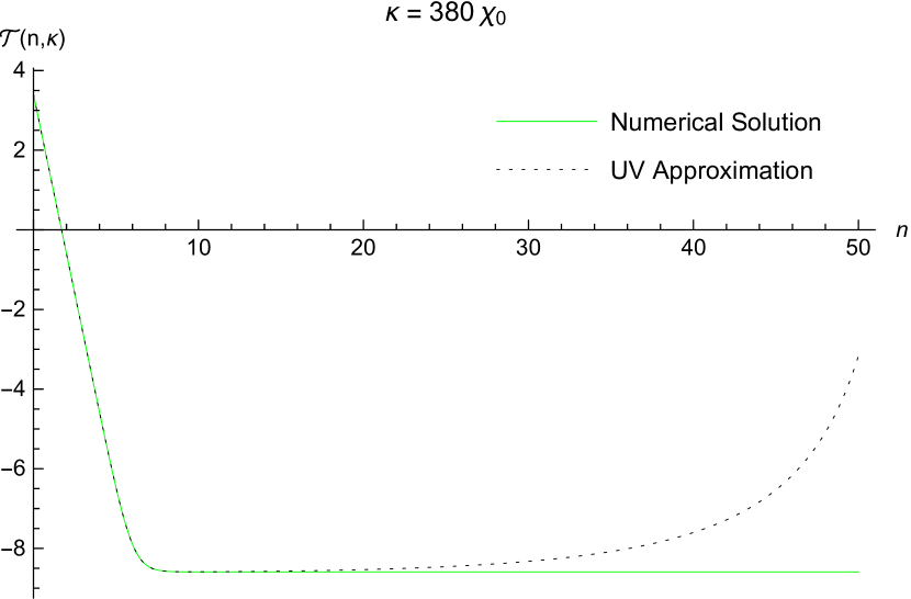
(a) $n_{\kappa}\simeq 6.0$

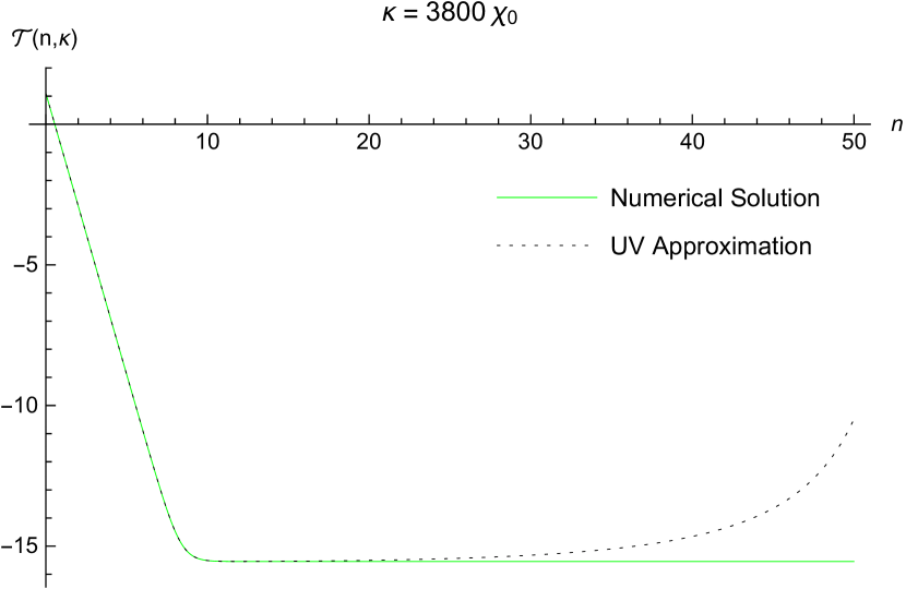
(b) $n_{\kappa}\simeq 8.3$

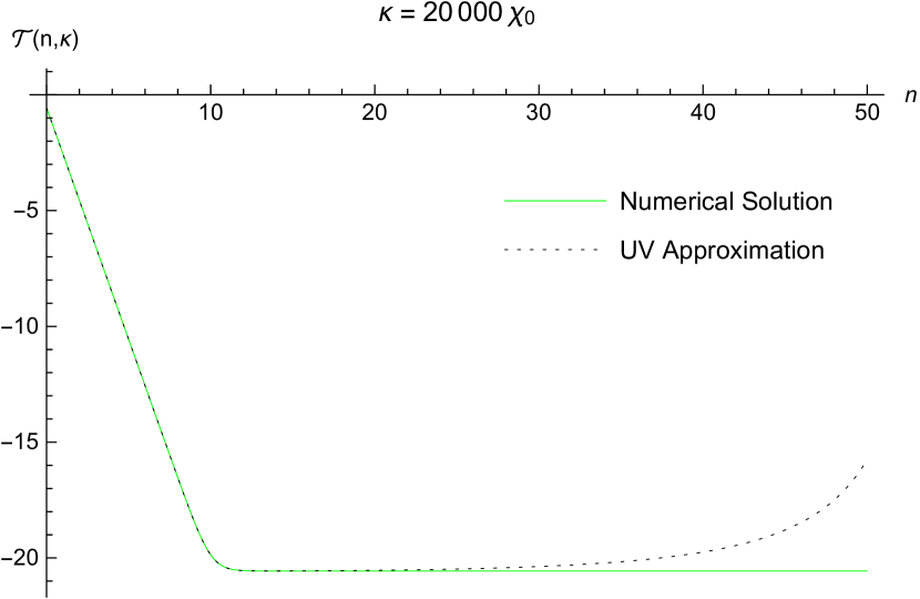
(c) $n_{\kappa}\simeq 10.0$

Figure 1: Plots the massless, minimally coupled scalar amplitude $\mathcal{T}(n,\kappa)$ (in solid green) and the (black dashed) ultraviolet approximation (109) versus the e-folding $n$ for three different values of $\kappa$.

Of course expression (109) is an approximation to the exact result. Because we propose to use this to compute the divergent coincidence limit of the propagator it is important to see how well $\mathcal{T}_{1}(n,\kappa)$ captures the ultraviolet behavior of $\mathcal{T}(n,\kappa)$. Because (109) is exact for constant first slow roll parameter, the deviation must involve derivatives of $\epsilon(n)$. It turns out to fall off like $\kappa^{-4}$ [24],

$$\mathcal{T}(n,\kappa)-\mathcal{T}_{1}(n,\kappa)=\Bigl{(}\frac{D\!-\!2}{16}\Bigr{)}\Bigl{[}(D+5-7\epsilon)\epsilon^{\prime}+\epsilon^{\prime\prime}\Bigr{]}\Bigl{(}\frac{\chi e^{n}}{\kappa}\Bigr{)}^{4}+O\Biggl{(}\Bigl{(}\frac{\chi e^{n}}{\kappa}\Bigr{)}^{6}\Biggr{)}.$$ (111)

We will see in section 4 that this suffices for an exact description of the ultraviolet.

The discrepancy between $\mathcal{T}(n,\kappa)$ and $\mathcal{T}_{1}(n,\kappa)$ that is evident at late times in Figure 1 is due to evolution of the first slow roll parameter $\epsilon(n)$. Figure 2 shows that the asymptotic late time phase is captured with great accuracy by the form,

$$\mathcal{T}_{2}(n,\kappa)=\ln\Biggl{[}\frac{\chi^{2}(n_{\kappa})}{2\kappa^{3}}\times C\Bigl{(}\epsilon(n_{\kappa})\Bigr{)}\Biggr{]}\;,$$ (112)

where the nearly unit correction factor $C(\epsilon)$ is,

$$C(\epsilon)\equiv\frac{1}{\pi}\Gamma^{2}\Bigl{(}\frac{1}{2}+\frac{1}{1\!-\!\epsilon}\Bigr{)}[2(1\!-\!\epsilon)]^{\frac{2}{1-\epsilon}}\;.$$ (113)

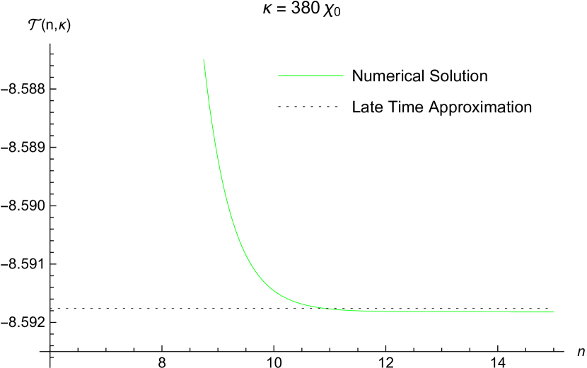
(a) $n_{\kappa}\simeq 6.0$

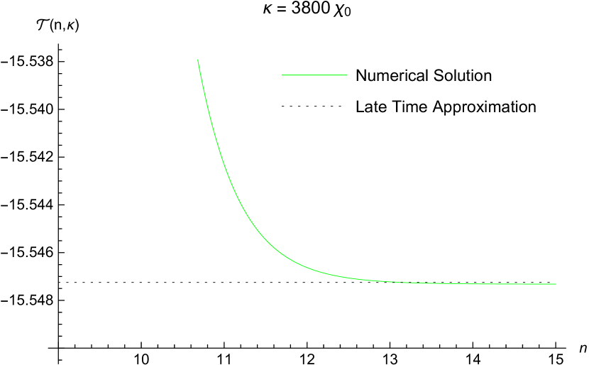
(b) $n_{\kappa}\simeq 8.3$

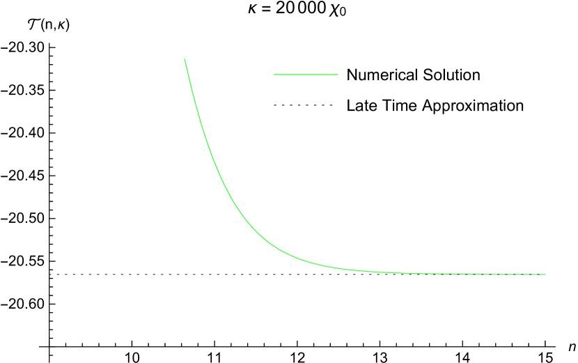
(c) $n_{\kappa}\simeq 10.0$

Figure 2: Plots the massless, minimally coupled scalar amplitude $\mathcal{T}(n,\kappa)$ (in solid green) and the (black dashed) late time approximation (112) versus the e-folding $n$ for three different values of $\kappa$.

Expression (112) is exact for constant $\epsilon(n)$. When the first slow roll parameter evolves there are very small nonlocal corrections whose form is known [25] but whose net contribution is negligible for smooth potentials.

3.3 Temporal Photon

The temporal photon amplitude is very similar to the massive scalar which was the subject of a previous study [26]. Like that system, the functional form of the amplitude is controlled by two key events:

1. First horizon crossing at $n_{\kappa}$ such that $\kappa e^{-n_{\kappa}}=\chi(n_{\kappa})$; and

2. Mass domination at $n_{\mu}$ such that $\mu=\frac{1}{2}\chi(n_{\mu})$.

The ultraviolet is well approximated by the form that applies for constant $\epsilon(n)$ and $\mu\propto\chi(n)$ [27],

$$\mathcal{U}_{1}(n,\kappa,\mu)\equiv\ln\Biggl{[}\frac{\frac{\pi}{2}z(n,\kappa)}{2\kappa e^{(D-2)n}}\Bigl{|}H^{(1)}_{\nu_{u}(n,\mu)}\Bigl{(}z(n,\kappa)\Bigr{)}\Bigr{|}^{2}\Biggr{]},$$ (114)

where the temporal index is,

$$\nu^{2}_{u}(n,\mu)\equiv\frac{1}{4}\Bigl{(}\frac{D\!-\!3\!+\!\epsilon(n)}{1\!-\!\epsilon(n)}\Bigr{)}^{2}\!\!-\frac{\mu^{2}}{[1\!-\!\epsilon(n)]^{2}\chi^{2}(n)}.$$ (115)

Figure 3 shows that the ultraviolet approximation is excellent when matter domination comes either before or after inflation.

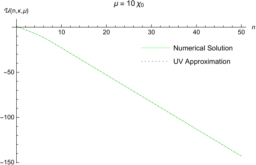
(a) $n_{\mu}<0$

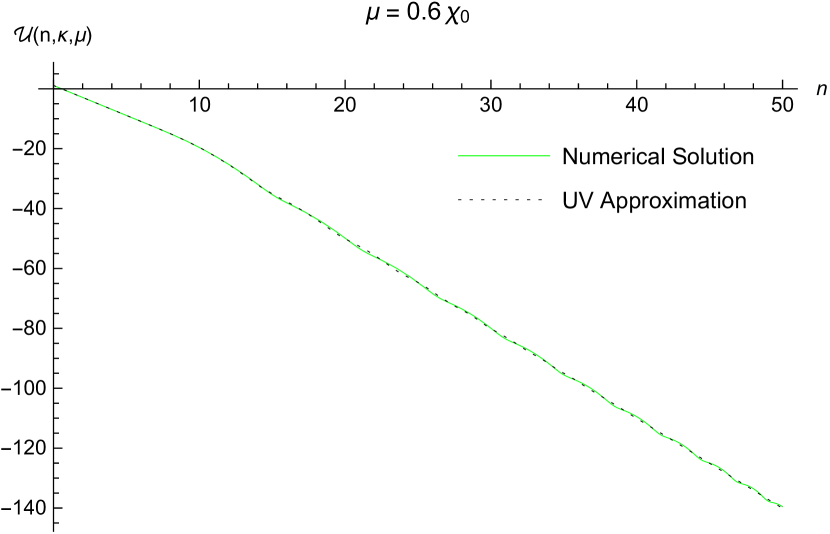
(b) $n_{\mu}<0$

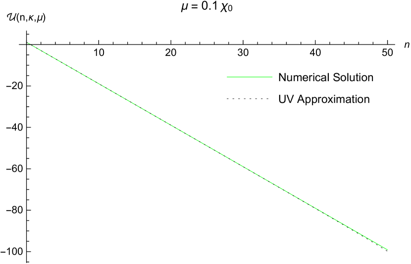
(c) $n_{\mu}>50$

Figure 3: Plots the temporal amplitude $\mathcal{U}(n,\kappa,\mu)$ and the ultraviolet approximation (114) versus the e-folding $n$ for $\kappa=3800\chi_{0}$ (with $n_{\kappa}\simeq 8.3$) and three different values of $\mu$ with outside the range of inflation.

The ultraviolet regime is $\kappa e^{-n}\gg\{\chi(n),\mu\}$. To see how well the ultraviolet approximation captures this regime we substitute the difference into the exact evolution equation (105) and expand in powers of $e^{n}\chi(n)/\kappa$ to find [26],

$$\mathcal{U}(n,\kappa,\mu)-\mathcal{U}_{1}(n,\kappa,\mu)=\Biggl{\{}\Bigl{(}5\epsilon-3\epsilon^{2}\Bigr{)}\frac{\mu^{2}}{4\chi^{2}}$$ (116)

$$\hskip 51.21504pt+\Bigl{(}\frac{D\!-\!2}{16}\Bigr{)}\Bigl{[}(D-9+7\epsilon)\epsilon^{\prime}-\epsilon^{\prime\prime}\Bigr{]}\Biggr{\}}\Bigl{(}\frac{\chi e^{n}}{\kappa}\Bigr{)}^{4}\!+O\Biggl{(}\Bigl{(}\frac{\chi e^{n}}{\kappa}\Bigr{)}^{6}\Biggr{)}.\qquad$$

This is suffices to give an exact result for the ultraviolet so we that can take the unregulated limit of $D=4$ for the approximations which pertain for $n>n_{\kappa}$.

The various terms in equation (105) behave differently before and after first horizon crossing. Evolution before first horizon crossing is controlled by the 4th and 7th terms,

$$\frac{2\kappa^{2}e^{-2n}}{\chi^{2}}-\frac{e^{-2(D-1)n-2\mathcal{U}}}{2\chi^{2}}\simeq 0\qquad\Longrightarrow\qquad\mathcal{U}\simeq-\ln(2\kappa)-(D\!-\!2)n\;.$$ (117)

After first horizon crossing these terms rapidly redshift into insignificance. We can take the unregulated limit ($D=4$), and equation (105) becomes,

$$\mathcal{U}^{\prime\prime}+\frac{1}{2}{\mathcal{U}^{\prime}}^{2}+(3\!-\!\epsilon)\mathcal{U}^{\prime}+4(1\!-\!\epsilon)+\frac{2\mu^{2}}{\chi^{2}}\simeq 0\;.$$ (118)

This is a nonlinear, first order equation for $\mathcal{U}^{\prime}$. Following [26] we make the ansatz,

$$\mathcal{U}^{\prime}\simeq\alpha+\beta\tanh(\gamma)\;.$$ (119)

Substituting (119) in (118) gives,

$$\Bigl{(}{\rm Eqn.\ \ref{scUlate}}\Bigr{)}=\alpha^{\prime}+\frac{1}{2}\alpha^{2}+\frac{1}{2}\beta^{2}+(3\!-\!\epsilon)\alpha+4(1\!-\!\epsilon)+\frac{2\mu^{2}}{\chi^{2}}$$ (120)

$$\hskip 76.82234pt+\Bigl{[}(3\!-\!\epsilon\!+\!\alpha)\beta+\beta^{\prime}\Bigr{]}\tanh(\gamma)+\beta\Bigl{(}\gamma^{\prime}-\frac{1}{2}\beta\Bigr{)}{\rm sech}^{2}(\gamma)\;.\qquad$$

Ansatz (119) does not quite solve (118), but the following choices reduce the residue to terms of order $\epsilon\times\tanh(\gamma)$,

$$\alpha=-3\qquad,\qquad\frac{1}{4}\beta^{2}=\frac{1}{4}+\frac{\epsilon}{2}-\frac{\mu^{2}}{\chi^{2}}\qquad,\qquad\gamma^{\prime}=\frac{1}{2}\beta\;.$$ (121)

Figures 4 and 5 show how $\mathcal{U}(n,\kappa,\mu)$ behaves when mass domination comes after first horizon crossing and before the end of inflation.

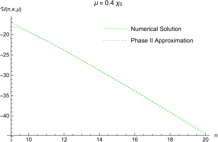
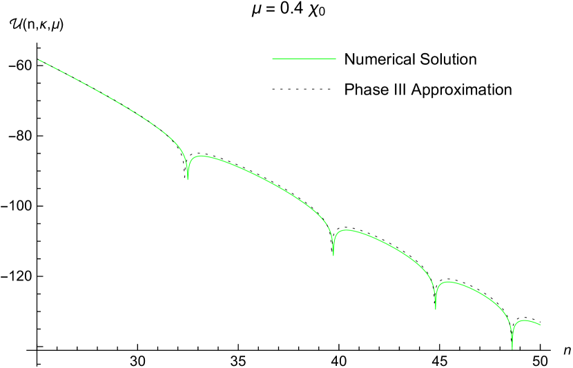
Figure 4: Plots the temporal amplitude $\mathcal{U}(n,3800\chi_{0},0.4\chi_{0})$ and the three approximations: (114), (123) and (124). For $\kappa=3800\chi_{0}$ horizon crossing occurs at $n_{\kappa}\simeq 8.3$; for $\mu=0.4\chi_{0}$ mass domination occurs at $n_{\mu}\simeq 20.2$.

First comes a phase of slow decline followed by a period of oscillations. From (119) with (121) we see that these phases are controlled by a “frequency” defined as,

$$\omega^{2}_{u}(n,\mu)\equiv\frac{1}{4}+\frac{\epsilon(n)}{2}-\frac{\mu^{2}}{\chi^{2}(n)}\equiv-\Omega^{2}_{u}(n,\mu)\;.$$ (122)

During the phase of slow decline $\omega^{2}_{u}(n,\mu)>0$. Integrating (119) with (121) for this case gives,

$$\mathcal{U}_{2}(n,\kappa,\mu)=\mathcal{U}_{2}-3(n\!-\!n_{2})+2\ln\Biggl{[}\cosh\Bigl{(}\int_{n_{2}}^{n}\!\!\!dn^{\prime}\omega_{u}(n^{\prime},\mu)\Bigr{)}$$ (123)

$$\hskip 142.26378pt+\Bigl{(}\frac{3\!+\!\mathcal{U}_{2}^{\prime}}{2\omega_{u}(n_{2},\mu)}\Bigr{)}\sinh\Bigl{(}\int_{n_{2}}^{n}\!\!\!dn^{\prime}\omega_{u}(n^{\prime},\mu)\Bigr{)}\Biggr{]},\qquad$$

where $n_{2}\equiv n_{\kappa}+4$. The oscillatory phase is characterized by $\omega^{2}_{u}(n,\mu)<0$. Integrating (119) with (121) for this case produces,

$$\mathcal{U}_{3}(n,\kappa,\mu)=\mathcal{U}_{3}-3(n\!-\!n_{3})+2\ln\Biggl{[}\Biggl{|}\cos\Bigl{(}\int_{n_{3}}^{n}\!\!\!dn^{\prime}\Omega_{u}(n^{\prime},\mu)\Bigr{)}$$ (124)

$$\hskip 142.26378pt+\Bigl{(}\frac{3\!+\!\mathcal{U}_{3}^{\prime}}{2\Omega_{u}(n_{3},\mu)}\Bigr{)}\sin\Bigl{(}\int_{n_{3}}^{n}\!\!\!dn^{\prime}\Omega_{u}(n^{\prime},\mu)\Bigr{)}\Biggr{|}\Biggr{]},\qquad$$

where $n_{3}\equiv n_{\mu}+4$. Figures 4 and 5 show that these approximations are excellent.

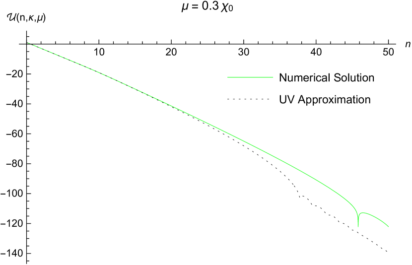
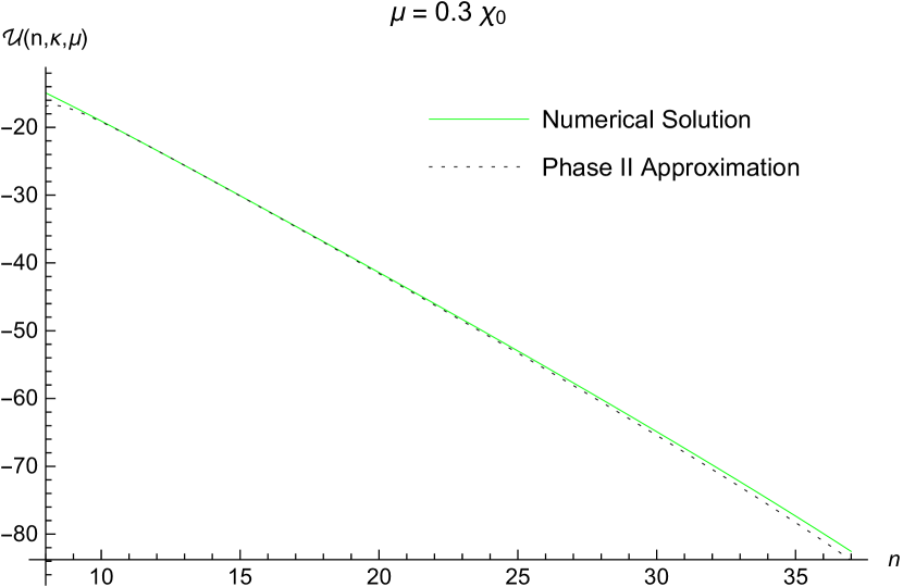
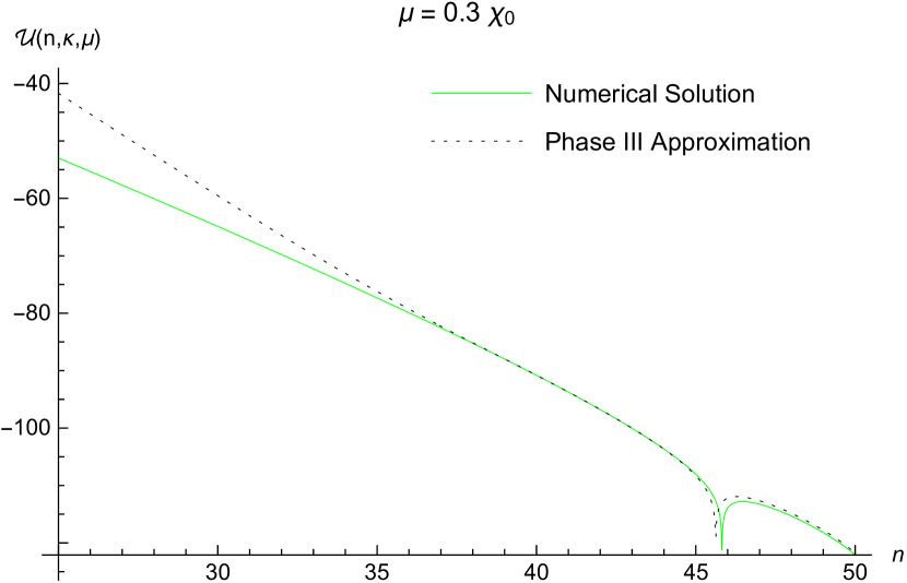
Figure 5: Plots the temporal amplitude $\mathcal{U}(n,3800\chi_{0},0.3\chi_{0})$ and the three approximations: (114), (123) and (124). For $\kappa=3800\chi_{0}$ horizon crossing occurs at $n_{\kappa}\simeq 8.3$; for $\mu=0.3\chi_{0}$ mass domination occurs at $n_{\mu}\simeq 36.0$.

It is worth noting that the approximations (123) and (124) depend on $\kappa$ principally through the integration constants $\mathcal{U}_{2}\equiv\mathcal{U}(n_{2},\kappa,\mu)$ and $\mathcal{U}_{3}\equiv\mathcal{U}(n_{3},\kappa,\mu)$. Figure 6 shows the difference $\mathcal{U}(n,400\chi_{0},\mu)-\mathcal{U}(n,3800\chi_{0},\mu)$ for the same two choices of $\mu$ in Figures 4 and 5. One can see that the difference freezes into a constant after first horizon crossing to better than five significant figures!

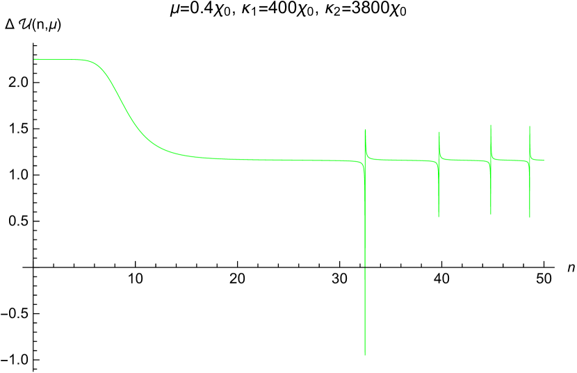
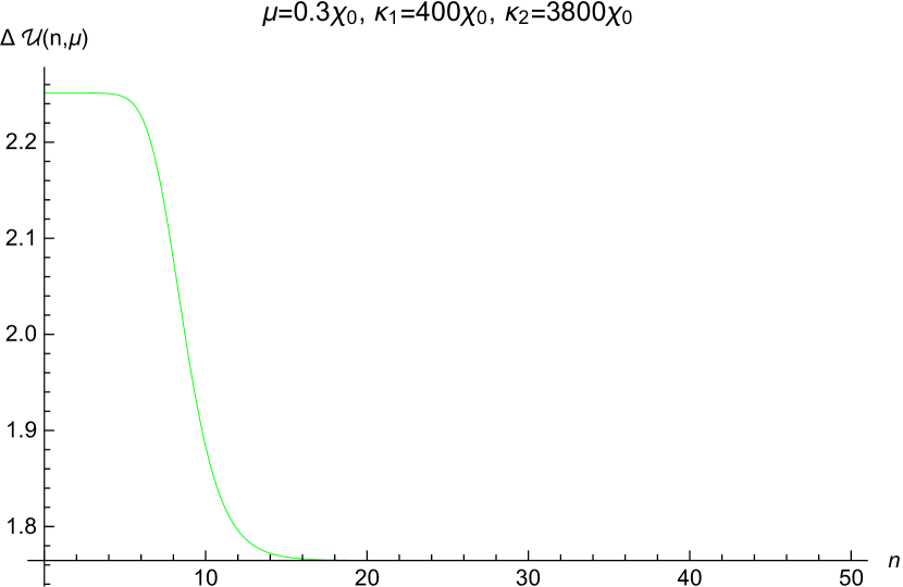
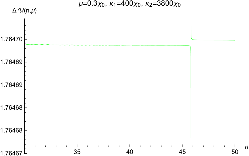
Figure 6: Plots the difference of the temporal amplitude $\Delta\mathcal{U}\equiv\mathcal{U}(n,\kappa_{1},\mu)-\mathcal{U}(n,\kappa_{2},\mu)$ for $\kappa_{1}=400\chi_{0}$ and $\kappa_{2}=3800\chi_{0}$ with $\mu$ chosen so that all three approximations (114), (123) and (124) are necessary.

3.4 Spatially Transverse Photons

The general considerations for the amplitude of spatially transverse photons are similar to those for temporal photons. Before first horizon crossing it is the 4th and last terms of equation (107) which control the evolution,

$$\frac{2\kappa^{2}e^{-2n}}{\chi^{2}}-\frac{e^{-2(D-3)n-2\mathcal{V}}}{2\chi^{2}}\simeq 0\qquad\Longrightarrow\qquad\mathcal{V}\simeq-\ln(2\kappa)-(D\!-\!4)n\;.$$ (125)

A more accurate approximation is,

$$\mathcal{V}_{1}(n,\kappa,\mu)\equiv\ln\Biggl{[}\frac{\frac{\pi}{2}z(n,\kappa)}{2\kappa e^{(D-4)n}}\Bigl{|}H^{(1)}_{\nu_{v}(n,\mu)}\Bigl{(}z(n,\kappa)\Bigr{)}\Bigr{|}^{2}\Biggr{]},$$ (126)

where $z(n,\kappa)$ is the same as (110) and the transverse index is,

$$\nu^{2}_{v}(n,\mu)\equiv\frac{1}{4}\Bigl{(}\frac{D\!-\!3\!-\!\epsilon(n)}{1\!-\!\epsilon(n)}\Bigr{)}^{2}-\frac{\mu^{2}}{[1\!-\!\epsilon(n)]^{2}\chi^{2}(n)}\;.$$ (127)

Note the slight (order $\epsilon$) difference between $\nu^{2}_{u}(n,\mu)$ and $\nu^{2}_{v}(n,\mu)$. Figure 7 shows that (126) is excellent up to several e-foldings after first horizon crossing, and throughout inflation for $n_{\mu}<0$.

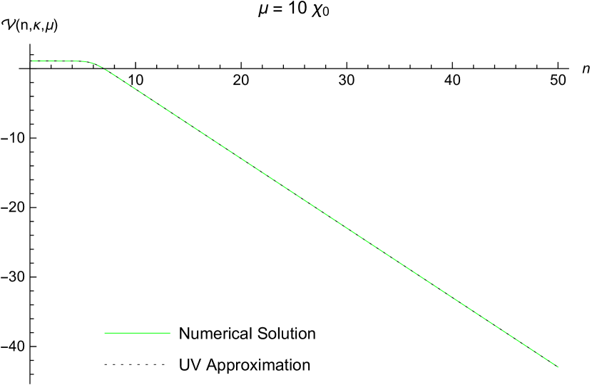
(a) $n_{\mu}<0$

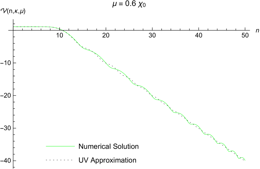
(b) $n_{\mu}<0$

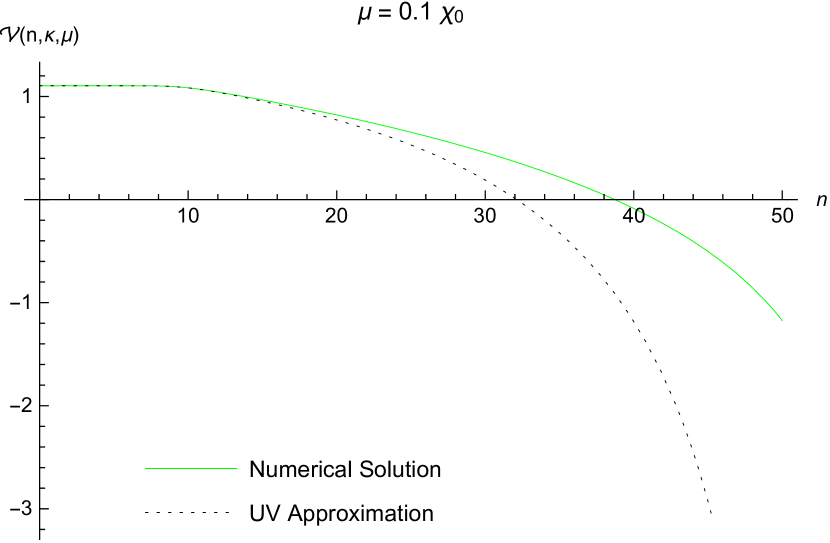
(c) $n_{\mu}>50$

Figure 7: Plots the transverse amplitude $\mathcal{V}(n,\kappa,\mu)$ and the ultraviolet approximation (126) versus the e-folding $n$ for $\kappa=3800\chi_{0}$ (with $n_{\kappa}\simeq 8.3$) and three different values of $\mu$ with outside the range of inflation.

Expression (126) also models the ultraviolet to high precision,

$$\mathcal{V}(n,\kappa,\mu)-\mathcal{V}_{1}(n,\kappa,\mu)=\Biggl{\{}\Bigl{(}5\epsilon-3\epsilon^{2}\Bigr{)}\frac{\mu^{2}}{4\chi^{2}}$$ (128)

$$\hskip 51.21504pt+\Bigl{(}\frac{D\!-\!4}{16}\Bigr{)}\Bigl{[}(D+3-7\epsilon)\epsilon^{\prime}+\epsilon^{\prime\prime}\Bigr{]}\Biggr{\}}\Bigl{(}\frac{\chi e^{n}}{\kappa}\Bigr{)}^{4}\!+O\Biggl{(}\Bigl{(}\frac{\chi e^{n}}{\kappa}\Bigr{)}^{6}\Biggr{)}.\qquad$$

Figure 8 shows $\mathcal{V}(n,\kappa,\mu)$ for the case where $n_{\mu}$ happens after first horizon crossing and before the end of inflation. One sees the same phases of slow decline after first horizon crossing, followed by oscillations.

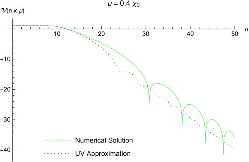
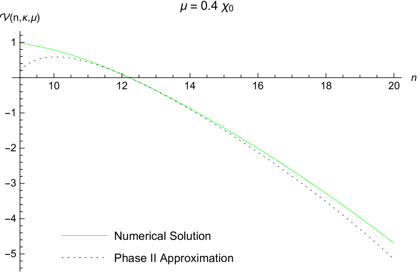
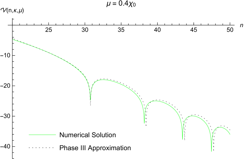
Figure 8: Plots the transverse amplitude $\mathcal{V}(n,3800\chi_{0},0.4\chi_{0})$ and the three approximations: (126), (131) and (132). For $\kappa=3800\chi_{0}$ horizon crossing occurs at $n_{\kappa}\simeq 8.3$; for $\mu=0.4\chi_{0}$ mass domination occurs at $n_{\mu}\simeq 20.2$.

The second and third phases can be understood by noting that the two terms of expression (125) redshift into insignificance after first horizon crossing. We can also set $D=4$ so that equation (107) degenerates to,

$$\mathcal{V}^{\prime\prime}+\frac{1}{2}{\mathcal{V}^{\prime}}^{2}+(1\!-\!\epsilon)\mathcal{V}^{\prime}+\frac{2\mu^{2}}{\chi^{2}}\simeq 0\;.$$ (129)

The same ansatz (119) applies to this regime, with the parameter choices,

$$\alpha=-1\quad,\quad\frac{1}{4}\beta^{2}=\frac{1}{4}-\frac{\mu^{2}}{\chi^{2}}\equiv\omega^{2}_{v}\equiv-\Omega^{2}_{v}\quad,\quad\gamma^{\prime}=\frac{1}{2}\beta\;.$$ (130)

Just as there was an order $\epsilon$ difference between the temporal and transverse indices — expressions (110) and (127), respectively — so too there is an order $\epsilon$ difference between $\omega^{2}_{u}(n,\mu)$ and $\omega^{2}_{v}(n,\kappa)$.

Integrating (119) with (130) for $\omega^{2}_{v}(,\mu)>0$ gives,

$$\mathcal{V}_{2}(n,\kappa,\mu)=\mathcal{V}_{2}-(n\!-\!n_{2})+2\ln\Biggl{[}\cosh\Bigl{(}\int_{n_{2}}^{n}\!\!\!dn^{\prime}\omega_{v}(n^{\prime},\mu)\Bigr{)}$$ (131)

$$\hskip 142.26378pt+\Bigl{(}\frac{1\!+\!\mathcal{V}_{2}^{\prime}}{2\omega_{v}(n_{2},\mu)}\Bigr{)}\sinh\Bigl{(}\int_{n_{2}}^{n}\!\!\!dn^{\prime}\omega_{v}(n^{\prime},\mu)\Bigr{)}\Biggr{]},\qquad$$

where $n_{2}\equiv n_{\kappa}+4$. Integrating (119) with (130) for $\omega^{2}_{v}(n,\mu)<0$ results in,

$$\mathcal{V}_{3}(n,\kappa,\mu)=\mathcal{V}_{3}-(n\!-\!n_{3})+2\ln\Biggl{[}\Biggl{|}\cos\Bigl{(}\int_{n_{3}}^{n}\!\!\!dn^{\prime}\Omega_{v}(n^{\prime},\mu)\Bigr{)}$$ (132)

$$\hskip 142.26378pt+\Bigl{(}\frac{1\!+\!\mathcal{V}_{3}^{\prime}}{2\Omega_{v}(n_{3},\mu)}\Bigr{)}\sin\Bigl{(}\int_{n_{3}}^{n}\!\!\!dn^{\prime}\Omega_{v}(n^{\prime},\mu)\Bigr{)}\Biggr{|}\Biggr{]},\qquad$$

where $n_{3}\equiv n_{\mu}+4$. Figures 8 and 9 demonstrate that the (131) and (132) approximations are excellent.

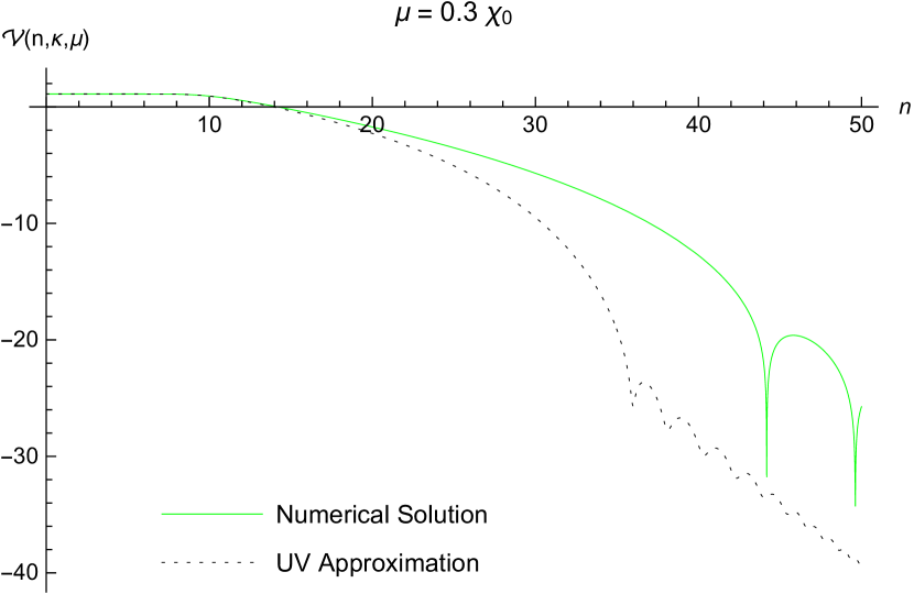
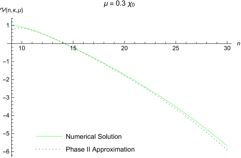
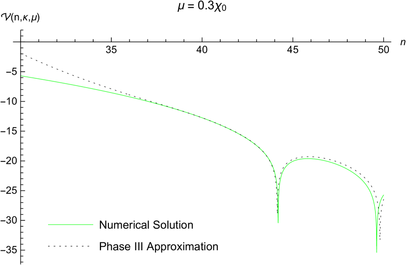
Figure 9: Plots the transverse amplitude $\mathcal{V}(n,3800\chi_{0},0.3\chi_{0})$ and the three approximations: (126), (131) and (132). For $\kappa=3800\chi_{0}$ horizon crossing occurs at $n_{\kappa}\simeq 8.3$; for $\mu=0.3\chi_{0}$ mass domination occurs at $n_{\mu}\simeq 36.0$.

Finally, we note that from Figure 10 that $\mathcal{V}^{\prime}(n,\kappa,\mu)$ is nearly independent of $\kappa$ after first horizon crossing.

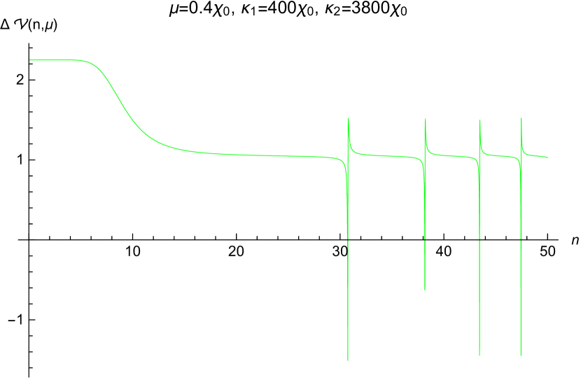
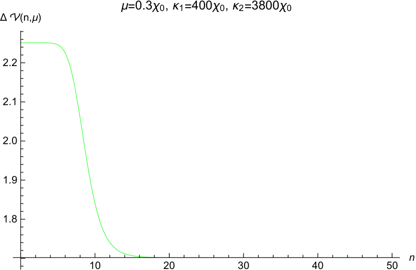
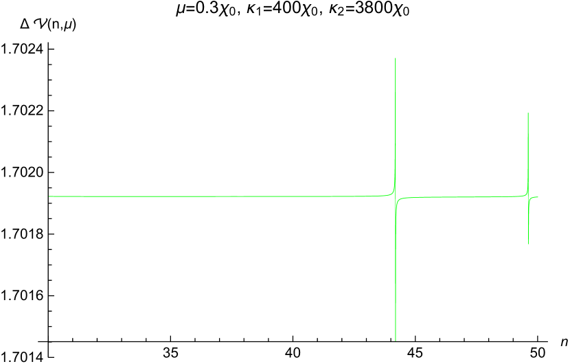
Figure 10: Plots the difference of the transverse amplitude $\Delta\mathcal{V}\equiv\mathcal{V}(n,\kappa_{1},\mu)-\mathcal{V}(n,\kappa_{2},\mu)$ for $\kappa_{1}=400\chi_{0}$ and $\kappa_{2}=3800\chi_{0}$ with $\mu$ chosen so that all three approximations (126), (131) and (132) are necessary.

One consequence for the (131) and (132) approximations is that only the integration constants $\mathcal{V}_{2}$ and $\mathcal{V}_{3}$ depend on $\kappa$.

3.5 Plateau Potentials

We chose the quadratic dimensionless potential $U(\psi\psi^{*})=c^{2}\psi\psi^{*}$ for detailed studies because it gives simple, analytic expressions (100) in the slow roll approximation for the dimensionless Hubble parameter $\chi(n)$ and the first slow roll parameter $\epsilon(n)$. Setting $c\simeq 7.126\times 10^{-6}$ makes this model consistent with the observed values for the scalar amplitude and the scalar spectral index [12]. On the other hand, the model’s large prediction of $r\simeq 0.14$ is badly discordant with limits on the tensor-to-scalar ratio [12]. We shall therefore briefly consider how our analytic approximations fare when used with the plateau potentials currently consistent with observation.

The best known plateau potential is the Einstein-frame version of Starobinsky’s famous $R+R^{2}$ model [13]. Expressing the dimensionless potential for this model in our notation gives [28],

$$U(\psi\psi^{*})=\frac{3}{4}M^{2}\Bigl{(}1-e^{-\sqrt{\frac{2}{3}}\,|\psi|}\Bigr{)}^{2}\qquad,\qquad M=1.3\times 10^{-5}\;.$$ (133)

Somewhat over 50 e-foldings of inflation result if one starts from $\psi_{0}=4.6$, and the choice of $M=1.3\times 10^{-5}$ makes the model consistent with observation [12]. Figure 11 shows why $r=16\epsilon$ is so small for this model: its dimensionless Hubble parameter $\chi(n)$ is nearly constant.

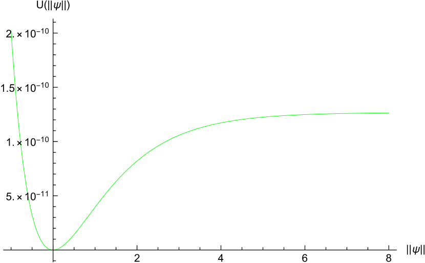
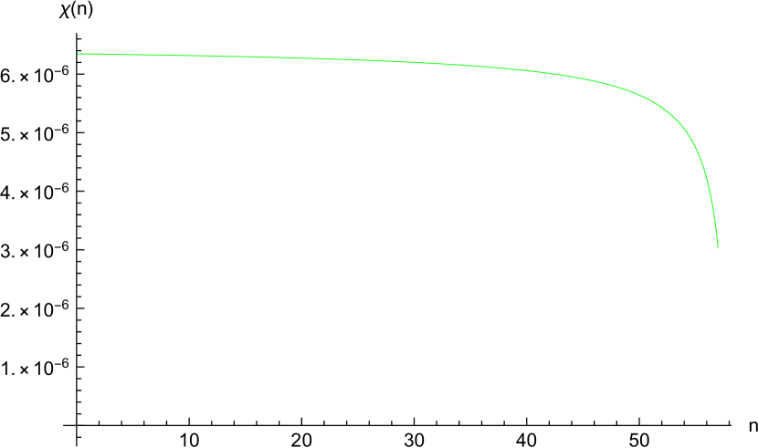
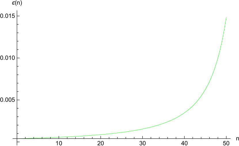
Figure 11: Potential and geometry for the Einstein-frame representation of Starobinsky’s original model of inflation [13]. The left shows the dimensionless potential $U(\psi\psi^{*})$ (133); the middle plot gives the dimensionless Hubble parameter $\chi(n)$ and the right hand plot depicts the first slow roll parameter $\epsilon(n)$. Inflation was assumed to start from $\psi_{0}=4.6$.

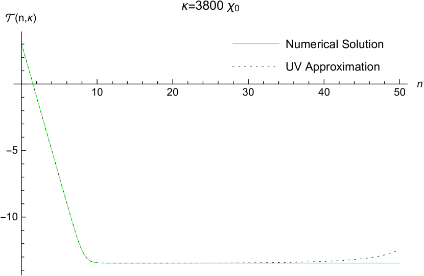
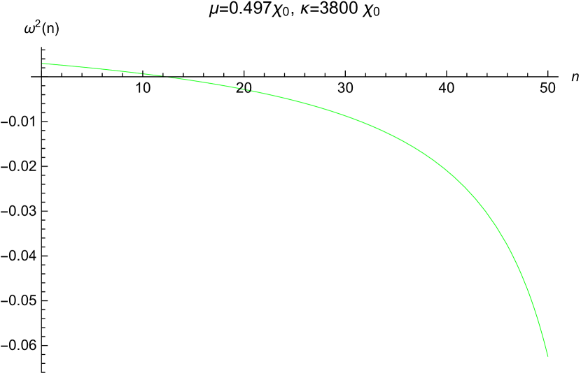
Figure 12: The left hand plot shows the amplitude $\mathcal{T}(n,\kappa)$ of the massless, minimally coupled scalar for $\kappa=3800\chi_{0}$, which corresponds to $n_{\kappa}\simeq 8.3$. The right hand graph shows the frequency $\omega_{u}^{2}(n,\mu)\simeq\omega^{2}_{v}(n,\mu)$ for $\mu=0.497\chi_{0}$ which passes through zero at $n_{\mu}\simeq 12$.

All our approximations pertain for this model, but the general effect of $\chi(n)$ being so nearly constant is to increase the range over which the ultraviolet approximations pertain. The left hand plot of Figure 12 shows this for the MMC scalar amplitude $\mathcal{T}(n,\kappa)$. Because $\epsilon(n)$ is so small, the temporal and transverse frequencies are nearly equal $\omega^{2}_{u}(n,\mu)\simeq\omega^{2}_{v}(n,\mu)$ and nearly constant. The right hand plot of Figure 12 shows this for a carefully chosen value of $\mu=0.497\chi_{0}$ which causes mass domination to occur during inflation. For this case we can just see the second and third phases occur in Figure 13.

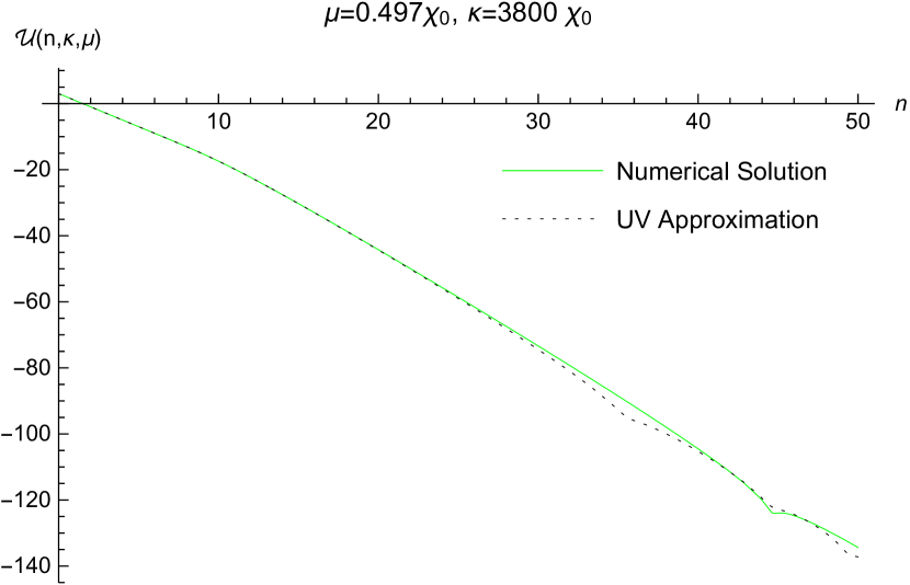
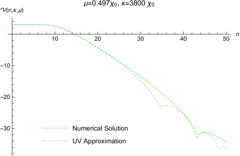
Figure 13: Plots of the temporal amplitude $\mathcal{U}(n,\kappa,\mu)$ (left) and the spatially transverse amplitude $\mathcal{V}(n,\kappa,\mu)$ (right) versus $n$ for the Starobinsky potential (133). For each amplitude $\kappa=3800\chi_{0}$ (which implies $n_{\kappa}\simeq 8.3$) and $\mu=0.497\chi_{0}$ (which implies $n_{\mu}\simeq 12$).

4 Effective Potential

The purpose of this section is to evaluate the one photon loop contribution to the inflaton effective potential defined by equation (6). We begin by deriving some exact results for the trace of the coincident propagator, and we recall that $\mathcal{T}(n,\kappa)$ can be obtained from $\mathcal{U}(n,\kappa,0)$. Then the ultraviolet approximations (114) and (126) are used to derive a divergent result whose renormalization gives the part of the effective potential that depends locally on the geometry. We give large field and small field expansions for this local part, and we study its dependence on derivatives of $\epsilon(n)$. The section closes with a discussion of the nonlocal part of the effective potential which derives from the late time approximations (123), (124), (131) and (132).

4.1 Trace of the Coincident Photon Propagator

At coincidence the mixed time-space components of the photon mode sum vanish, and factors of $\widehat{k}_{m}\widehat{k}_{n}$ average to $\delta_{mn}/(D-1)$,

$$i\Bigl{[}\mbox{}_{\mu}\Delta_{\nu}\Bigr{]}(x;x)=\int\!\!\frac{d^{D-1}k}{(2\pi)^{D-1}}\,\Biggl{\{}\frac{1}{M^{2}}\left(\matrix{k^{2}uu^{*}&0\cr 0&\frac{\delta_{mn}}{D-1}\mathcal{D}u\mathcal{D}u^{*}}\right)$$ (134)

$$\hskip 51.21504pt-\frac{1}{M^{2}}\left(\matrix{\partial_{0}t\partial_{0}t^{*}&0\cr 0&\frac{\delta_{mn}}{D-1}k^{2}tt^{*}}\right)+\left(\matrix{0&0\cr 0&(\frac{D-2}{D-1})\delta_{mn}vv^{*}}\right)\Biggr{\}}.\qquad$$

Its trace is,

$$g^{\mu\nu}i\Bigl{[}\mbox{}_{\mu}\Delta_{\nu}\Bigr{]}(x;x)=$$ (135)

$$\hskip 28.45274pt\int\!\!\frac{d^{D-1}k}{(2\pi)^{D-1}}\,\Biggl{\{}\frac{\mathcal{D}u\mathcal{D}u^{*}\!-\!k^{2}uu^{*}\!+\!\partial_{0}t\partial_{0}t^{*}\!-\!k^{2}tt^{*}}{a^{2}M^{2}}+\frac{(D\!-\!2)vv^{*}}{a^{2}}\Biggr{\}}.\qquad$$

Relation (55) allows us to replace the MMC scalar mode function $t(\eta,k)$ with the massless limit of the temporal mode function $u_{0}(\eta,k)\equiv u(\eta,k,0)$,

$$\partial_{0}t\partial_{0}t^{*}=k^{2}u_{0}u^{*}_{0}\qquad,\qquad k^{2}tt^{*}=\mathcal{D}u_{0}\mathcal{D}u^{*}_{0}\;.$$ (136)

Substituting (136) in (135) gives,

$$g^{\mu\nu}i\Bigl{[}\mbox{}_{\mu}\Delta_{\nu}\Bigr{]}(x;x)=$$ (137)

$$\hskip 22.76228pt\int\!\!\frac{d^{D-1}k}{(2\pi)^{D-1}}\,\Biggl{\{}\frac{\mathcal{D}u\mathcal{D}u^{*}\!-\!\mathcal{D}u_{0}\mathcal{D}u_{0}^{*}\!-\!k^{2}(uu^{*}\!-\!u_{0}u^{*}_{0})}{a^{2}M^{2}}+\frac{(D\!-\!2)vv^{*}}{a^{2}}\Biggr{\}}.\qquad$$

This second form (137) is very important because it demonstrates the absence of any $1/M^{2}$ pole as an exact relation, before any approximations are made.

The mode equation for temporal photons implies,

$$\mathcal{D}u\mathcal{D}u^{*}=a^{2}H^{2}\Bigl{[}u^{\prime}{u^{\prime}}^{*}+(D\!-\!2)(uu^{*})^{\prime}+(D\!-\!2)^{2}uu^{*}\Bigr{]}\;,$$ (139)

$$\hskip 22.76228pt=(k^{2}+a^{2}M^{2})uu^{*}+\frac{a^{2}H^{2}}{2}\Bigl{(}\partial_{n}\!+\!D\!-\!1\!-\!\epsilon\Bigr{)}\Bigl{(}\partial_{n}\!+\!2D\!-\!4\Bigr{)}(uu^{*})\;.\qquad$$

Using relations (139) and (137) allows us to express the trace of the coincident photon propagator in terms of three coincident scalar propagators,

$$g^{\mu\nu}i\Bigl{[}\mbox{}_{\mu}\Delta_{\nu}\Bigr{]}(x;x)=i\Delta_{u}(x;x)+\frac{(D\!-\!2)}{a^{2}}i\Delta_{v}(x;x)$$ (140)

$$\hskip 28.45274pt+\frac{H^{2}}{2M^{2}}\Bigl{(}\partial_{n}\!+\!D\!-\!1\!-\!\epsilon\Bigr{)}\Bigl{(}\partial_{n}\!+\!2D\!-\!4\Bigr{)}\Bigl{[}i\Delta_{u}(x;x)-i\Delta_{u_{0}}(x;x)\Bigr{]}\;.\qquad$$

The disappearance of any factors of $k^{2}$ from the Fourier mode sums in (140), coupled with the ultraviolet expansions (116) and (128), means that the phase 1 approximations $\mathcal{U}_{1}(n,\kappa,\mu)$ and $\mathcal{V}_{1}(n,\kappa,\mu)$ exactly reproduce the ultraviolet divergence structures.

Two of the scalar propagators in expression (140) are,

$$i\Delta_{u}(x;x^{\prime})\equiv\int\!\!\frac{d^{D-1}k}{(2\pi)^{D-1}}\Biggl{\{}\theta(\Delta\eta)u(\eta,k,M)u^{*}(\eta^{\prime},k,M)e^{i\vec{k}\cdot\Delta\vec{x}}$$ (141)

$$\hskip 128.0374pt+\theta(-\Delta\eta)u^{*}(\eta,k,M)u(\eta^{\prime},k,M)e^{-i\vec{k}\cdot\Delta\vec{x}}\Biggr{\}},\qquad$$

$$i\Delta_{v}(x;x^{\prime})\equiv\int\!\!\frac{d^{D-1}k}{(2\pi)^{D-1}}\Biggl{\{}\theta(\Delta\eta)v(\eta,k,M)v^{*}(\eta^{\prime},k,M)e^{i\vec{k}\cdot\Delta\vec{x}}$$ (142)

$$\hskip 128.0374pt+\theta(-\Delta\eta)v^{*}(\eta,k,M)v(\eta^{\prime},k,M)e^{-i\vec{k}\cdot\Delta\vec{x}}\Biggr{\}}.\qquad$$

The third scalar propagator $i\Delta_{u_{0}}(x;x^{\prime})$ is just the $M\rightarrow 0$ limit of $i\Delta_{u}(x;x^{\prime})$. The coincidence limits of each propagator can be expressed in terms of the corresponding amplitude,

$$\frac{i\Delta_{u}(x;x)}{\sqrt{8\pi G}}=\int\!\!\frac{d^{D-1}k}{(2\pi)^{D-1}}\,e^{\mathcal{U}(n,\kappa,\mu)}\quad,\quad\frac{i\Delta_{v}(x;x)}{\sqrt{8\pi G}}=\int\!\!\frac{d^{D-1}k}{(2\pi)^{D-1}}\,e^{\mathcal{V}(n,\kappa,\mu)}\;.$$ (143)

Expression(140) is exact but not immediately useful because we lack explicit expressions for the coincident propagators (143). It is at this stage that we must resort to the analytic approximations developed in section 3. Recall that the phase 1 approximation is valid until roughly 4 e-foldings after horizon crossing. If one instead thinks of this as a condition on the dimensionless wave number $\kappa\equiv\sqrt{8\pi G}\,k$ at fixed $n$, it means that $\kappa>\kappa_{n-4}$, where we define $\kappa_{n}$ as the dimensionless wave number which experiences horizon crossing at e-folding $n$. Taking as an example the temporal photon contribution we can write,

$$e^{\mathcal{U}(n,\kappa,\mu)}\simeq\theta\Bigl{(}\kappa\!-\!\kappa_{n-4}\Bigr{)}e^{\mathcal{U}_{1}(n,\kappa,\mu)}+\theta\Bigl{(}\kappa_{n-4}-\kappa\Bigr{)}e^{\mathcal{U}_{2,3}(n,\kappa,\mu)}\;,$$ (145)

$$\hskip 56.9055pt=e^{\mathcal{U}_{1}(n,\kappa,\mu)}+\theta\Bigl{(}\kappa_{n-4}-\kappa\Bigr{)}\Biggl{[}e^{\mathcal{U}_{2,3}(n,\kappa,\mu)}-e^{\mathcal{U}_{1}(n,\kappa,\mu)}\Biggr{]}.\qquad$$

Substituting the approximation (145) into expression (143) allows us to write,

$$i\Delta_{u}(x;x)\simeq L_{u}(n)+N_{u}(n)\;,$$ (146)

where we define the local ($L$) and nonlocal ($N$) contributions as,

$$L_{u}(n) \!\!\!\equiv\!\!\! \sqrt{8\pi G}\!\int\!\!\frac{d^{D-1}k}{(2\pi)^{D-1}}\,e^{\mathcal{U}_{1}(n,\kappa,\mu)}\;,$$ (147)

$$N_{u}(n) \!\!\!\equiv\!\!\! \sqrt{8\pi G}\!\int\!\!\frac{d^{3}k}{(2\pi)^{3}}\,\theta\Bigl{(}\kappa_{n-4}-\kappa\Bigr{)}\Biggl{[}e^{\mathcal{U}_{2,3}(n,\kappa,\mu)}-e^{\mathcal{U}_{1}(n,\kappa,\mu)}\Biggr{]}.\qquad$$ (148)

Note that we have taken the unregulated limit ($D=4$) in expression (148) because it is ultraviolet finite. The same considerations apply as well for the coincident spatially transverse photon propagator $i\Delta_{v}(x;x^{\prime})$, and for the massless limit of the temporal photon propagator $i\Delta_{u_{0}}(x;x)$.

4.2 The Local Contribution

The local contribution for each of the coincident propagators (143) comes from using the phase 1 approximation (147). For the temporal modes the amplitude is approximated by expression (114), whereupon we change variables to $z$ using $k=(1-\epsilon)Haz$, and then employ integral $6.574\;\#2$ of [29],

$$L_{u}(n)=\frac{[(1\!-\!\epsilon)H]^{D-2}}{(4\pi)^{\frac{D}{2}}}\times\frac{\Gamma(\frac{D-1}{2}\!+\!\nu_{u})\Gamma(\frac{D-1}{2}\!-\!\nu_{u})}{\Gamma(\frac{1}{2}\!+\!\nu_{u})\Gamma(\frac{1}{2}\!-\!\nu_{u})}\times\Gamma\Bigl{(}1\!-\!\frac{D}{2}\Bigr{)}\;.$$ (149)

Recall that the index $\nu_{u}(n,\mu)$ is defined in expression (115). Of course the massless limit is,

$$L_{u_{0}}(n)=\frac{[(1\!-\!\epsilon)H]^{D-2}}{(4\pi)^{\frac{D}{2}}}\times\frac{\Gamma(\frac{D-1}{2}\!+\!\nu_{u_{0}})\Gamma(\frac{D-1}{2}\!-\!\nu_{u_{0}})}{\Gamma(\frac{1}{2}\!+\!\nu_{u_{0}})\Gamma(\frac{1}{2}\!-\!\nu_{u_{0}})}\times\Gamma\Bigl{(}1\!-\!\frac{D}{2}\Bigr{)}\;,$$ (150)

where the index is,

$$\nu_{u_{0}}(n)\equiv\nu_{u}(n,0)=\frac{1}{2}\Bigl{(}\frac{D\!-\!3\!+\!\epsilon(n)}{1\!-\!\epsilon(n)}\Bigr{)}\;.$$ (151)

The phase 1 approximation (126) for the transverse amplitude contains two extra scale factors which serve to exactly cancel the inverse scale factors that are evident in the transverse contribution to the trace of the coincident photon propagator (140). Hence we have,

$$\frac{L_{v}(n)}{a^{2}}=\frac{[(1\!-\!\epsilon)H]^{D-2}}{(4\pi)^{\frac{D}{2}}}\times\frac{\Gamma(\frac{D-1}{2}\!+\!\nu_{v})\Gamma(\frac{D-1}{2}\!-\!\nu_{v})}{\Gamma(\frac{1}{2}\!+\!\nu_{v})\Gamma(\frac{1}{2}\!-\!\nu_{v})}\times\Gamma\Bigl{(}1\!-\!\frac{D}{2}\Bigr{)}\;,$$ (152)

where the transverse index $\nu_{v}(n,\mu)$ is given in (127).

Each of the local contributions (149), (150) and (152) is proportional to the same divergent Gamma function,

$$\Gamma\Bigl{(}1\!-\!\frac{D}{2}\Bigr{)}=\frac{2}{D\!-\!4}+O\Bigl{(}(D\!-\!4)^{0}\Bigr{)}\;.$$ (153)

Each also contains a similar ratio of Gamma functions,

$$\frac{\Gamma(\frac{D-1}{2}\!+\!\nu)\Gamma(\frac{D-1}{2}\!-\!\nu)}{\Gamma(\frac{1}{2}\!+\!\nu)\Gamma(\frac{1}{2}\!-\!\nu)}=\Bigl{[}\Bigl{(}\frac{D\!-\!3}{2}\Bigr{)}^{2}\!-\!\nu^{2}\Bigr{]}\!\times\!\frac{\Gamma(\frac{D-3}{2}\!+\!\nu)\Gamma(\frac{D-3}{2}\!-\!\nu)}{\Gamma(\frac{1}{2}\!+\!\nu)\Gamma(\frac{1}{2}\!-\!\nu)}\;,$$ (155)

$$=\!\Bigl{[}\Bigl{(}\frac{D\!-\!3}{2}\Bigr{)}^{2}\!\!\!-\!\nu^{2}\Bigr{]}\Biggl{\{}\!1+\Bigl{[}\psi\Bigl{(}\frac{1}{2}\!+\!\nu\!\Bigr{)}\!+\!\psi\Bigl{(}\frac{1}{2}\!-\!\nu\!\Bigr{)}\Bigr{]}\Bigl{(}\frac{D\!-\!4}{2}\Bigr{)}\!+\!O\Bigl{(}(D\!-\!4)^{2}\Bigr{)}\!\Biggr{\}}.\qquad$$

These considerations allow us to break up each of the three terms in (140) into a potentially divergent part plus a manifestly finite part. For $i\Delta_{u}(x;x)\rightarrow L_{u}(n)$ this decomposition is,

$$L_{u}=\frac{[(1\!-\!\epsilon)H]^{D-4}}{(4\pi)^{\frac{D}{2}}}\Biggl{[}M^{2}-\frac{(D\!-\!2)H^{2}}{2}\Bigl{(}(D\!-\!3)\epsilon-\frac{1}{2}(D\!-\!4)\epsilon^{2}\Bigr{)}\Biggr{]}\Gamma\Bigl{(}1\!-\!\frac{D}{2}\Bigr{)}$$ (156)

$$\hskip 42.67912pt+\frac{1}{16\pi^{2}}\Bigl{[}M^{2}-\epsilon H^{2}\Bigr{]}\Bigl{[}\psi\Bigl{(}\frac{1}{2}\!+\!\nu_{u}\Bigr{)}+\psi\Bigl{(}\frac{1}{2}\!-\!\nu_{u}\Bigr{)}\Bigr{]}+O(D\!-\!4)\;.\qquad$$

For $(D-2)i\Delta_{v}(x;x)\rightarrow(D-2)L_{v}(n)$ we have,

$$(D\!-\!2)L_{v}=\frac{[(1\!-\!\epsilon)H]^{D-4}}{(4\pi)^{\frac{D}{2}}}\Biggl{[}(D\!-\!2)M^{2}-\frac{(D\!-\!2)(D\!-\!4)H^{2}}{2}\Bigl{(}(D\!-\!3)\epsilon$$ (157)

$$-\frac{(D\!-\!2)\epsilon^{2}}{2}\Bigr{)}\Biggr{]}\Gamma\Bigl{(}1\!-\!\frac{D}{2}\Bigr{)}+\frac{2M^{2}}{16\pi^{2}}\Bigl{[}\psi\Bigl{(}\frac{1}{2}\!+\!\nu_{v}\Bigr{)}+\psi\Bigl{(}\frac{1}{2}\!-\!\nu_{v}\Bigr{)}\Bigr{]}+O(D\!-\!4)\;.\qquad$$

And the final term in (140) — the one with derivatives — becomes,

$$\frac{H^{2}}{2M^{2}}\Bigl{(}\partial_{n}\!+\!D\!-\!1\!-\!\epsilon\Bigr{)}\Bigl{(}\partial_{n}\!+\!2D\!-\!4\Bigr{)}\Bigl{[}L_{u}\!-\!L_{u_{0}}\Bigr{]}=\frac{H^{2}}{2}\Bigl{(}\partial_{n}\!+\!D\!-\!1\!-\!\epsilon\Bigr{)}$$ (158)

$$\times\Bigl{(}\partial_{n}\!+\!2D\!-\!4\Bigr{)}\frac{[(1\!-\!\epsilon)H]^{D-4}}{(4\pi)^{\frac{D}{2}}}\Gamma\Bigl{(}1\!-\!\frac{D}{2}\Bigr{)}+\frac{H^{2}}{32\pi^{2}}\Bigl{(}\partial_{n}\!+\!3\!-\!\epsilon\Bigr{)}\Bigl{(}\partial_{n}\!+\!4\Bigr{)}\qquad$$

$$\hskip 28.45274pt\times\Biggl{\{}\psi\Bigl{(}\frac{1}{2}\!+\!\nu_{u}\Bigr{)}+\psi\Bigl{(}\frac{1}{2}\!-\!\nu_{u}\Bigr{)}-\frac{\epsilon H^{2}}{M^{2}}\Bigl{[}\psi\Bigl{(}\frac{1}{2}\!+\!\nu_{u}\Bigr{)}-\psi\Bigl{(}\frac{1}{2}\!+\!\nu_{u_{0}}\Bigr{)}$$

$$\hskip 128.0374pt+\psi\Bigl{(}\frac{1}{2}\!-\!\nu_{u}\Bigr{)}-\psi\Bigl{(}\frac{1}{2}\!-\!\nu_{u_{0}}\Bigr{)}\Bigr{]}\Biggr{\}}+O(D\!-\!4)\;.\qquad$$

Note that the difference $\psi(\frac{1}{2}\pm\nu_{u})-\psi(\frac{1}{2}\pm\nu_{u_{0}})$ is of order $M^{2}$ so expression (158) has no $1/M^{2}$ pole. Note also that the $1/\epsilon$ pole in $\psi(\frac{1}{2}-\nu_{u_{0}})=\psi(\frac{-\epsilon}{1-\epsilon})$ is canceled by an explicit multiplicative factor of $\epsilon$.

The potentially divergent terms (the ones proportional to $\Gamma(1-\frac{D}{2})$) in expressions (156), (157 and (158) sum to give,

$$(\ref{1stterm})_{\rm div}+(\ref{2ndterm})_{\rm div}+(\ref{3rdterm})_{\rm div}=\frac{[(1\!-\!\epsilon)H]^{D-4}}{(4\pi)^{\frac{D}{2}}}\Bigl{[}(D\!-\!1)M^{2}+\frac{1}{2}R\Bigr{]}\Gamma\Bigl{(}1\!-\!\frac{D}{2}\Bigr{)}$$ (159)

$$\hskip 19.91684pt+\frac{H^{2}}{16\pi^{2}}\Bigl{[}3-12\epsilon+4\epsilon^{2}-2\epsilon^{\prime}-\frac{(6\epsilon^{\prime}\!+\!\epsilon^{\prime\prime})}{1\!-\!\epsilon}-\Bigl{(}\frac{\epsilon^{\prime}}{1\!-\!\epsilon}\Bigr{)}^{2}\Bigr{]}+O(D\!-\!4)\;,\qquad$$

where we recall that the $D$-dimensional Ricci scalar is $R=(D-1)(D-2\epsilon)H^{2}$. Comparison with expression (6) for $\Delta V^{\prime}(\varphi\varphi^{*})$ reveals that we can absorb the divergences with the following counterterms,

$$\delta\xi=-\frac{\Gamma(1\!-\!\frac{D}{2})s^{D-4}}{(4\pi)^{\frac{D}{2}}}\times\frac{1}{2}q^{2}\qquad,\qquad\delta\lambda=-\frac{\Gamma(1\!-\!\frac{D}{2})s^{D-4}}{(4\pi)^{\frac{D}{2}}}\times 4(D\!-\!1)q^{4}\;,$$ (160)

where $s$ is the renormalization scale. Up to finite renormalizations, these choices agree with previous results [5, 6, 7], in the same gauge and using the same regularization, on de Sitter background.

Substituting expressions (156), (157), (158) and (160) into the definition (6) of $\Delta V^{\prime}(\varphi\varphi^{*})$ and taking the unregulated limit gives the local contribution,

$$\Delta V^{\prime}_{\rm L}(\varphi\varphi^{*})=\frac{q^{2}H^{2}}{16\pi^{2}}\Biggl{\{}\frac{(6M^{2}\!+\!R)}{2H^{2}}\ln\Bigl{[}\frac{(1\!-\!\epsilon)^{2}H^{2}}{s^{2}}\Bigr{]}\!+\!3\!-\!12\epsilon\!+\!4\epsilon^{2}\!-\!2\epsilon^{\prime}\!-\!\frac{(6\epsilon^{\prime}\!+\!\epsilon^{\prime\prime})}{1\!-\!\epsilon}$$ (161)

$$-\Bigl{(}\frac{\epsilon^{\prime}}{1\!-\!\epsilon}\Bigr{)}^{2}+\frac{M^{2}}{H^{2}}\Biggl{[}\psi\Bigl{(}\frac{1}{2}\!+\!\nu_{u}\Bigr{)}+\psi\Bigl{(}\frac{1}{2}\!-\!\nu_{u}\Bigr{)}+2\psi\Bigl{(}\frac{1}{2}\!+\!\nu_{v}\Bigr{)}+2\psi\Bigl{(}\frac{1}{2}\!-\!\nu_{v}\Bigr{)}\Biggr{]}$$

$$+\frac{1}{2}\Bigl{[}(\partial_{n}\!+\!3\!-\!\epsilon)(\partial_{n}\!+\!4)-2\epsilon\Bigr{]}\Bigl{[}\psi\Bigl{(}\frac{1}{2}\!+\!\nu_{u}\Bigr{)}\!+\!\psi\Bigl{(}\frac{1}{2}\!-\!\nu_{u}\Bigr{)}\Bigr{]}-(\partial_{n}\!+\!3\!-\!\epsilon)(\partial_{n}\!+\!4)$$

$$\hskip 51.21504pt\times\frac{\epsilon H^{2}}{2M^{2}}\Bigl{[}\psi\Bigl{(}\frac{1}{2}\!+\!\nu_{u}\Bigr{)}\!-\!\psi\Bigl{(}\frac{1}{1\!-\!\epsilon}\Bigr{)}+\psi\Bigl{(}\frac{1}{2}\!-\!\nu_{u}\Bigr{)}\!-\!\psi\Bigl{(}\frac{-\epsilon}{1\!-\!\epsilon}\Bigr{)}\Bigr{]}\Biggr{\}}.\qquad$$

It is worth noting that there are no singularities at $\epsilon=1$, or when either $1/(1-\epsilon)$ or $-\epsilon/(1-\epsilon)$ become non-positive integers [14]. The effective potential is obtained by integrating (161) with respect to $\varphi\varphi^{*}$. The result is best expressed using the variable $z\equiv q^{2}\varphi\varphi^{*}/H^{2}$,

$$\Delta V_{\rm L}=\frac{H^{4}}{16\pi^{2}}\Biggl{\{}\!\Bigl{[}3z^{2}\!+\!\frac{Rz}{2H^{2}}\Bigr{]}\!\ln\Bigl{[}\frac{(1\!-\!\epsilon)^{2}H^{2}}{s^{2}}\Bigr{]}\!+\!\Bigl{[}3\!-\!12\epsilon\!+\!4\epsilon^{2}\!-\!2\epsilon^{\prime}\!-\!\frac{(6\epsilon^{\prime}\!+\!\epsilon^{\prime\prime})}{1\!-\!\epsilon}\Bigr{]}z$$ (162)

$$-\frac{{\epsilon^{\prime}}^{2}z}{(1\!-\!\epsilon)^{2}}+2\!\int_{0}^{z}\!\!\!dx\,x\Biggl{[}\psi\Bigl{(}\frac{1}{2}\!+\!\alpha\!\Bigr{)}\!+\!\psi\Bigl{(}\frac{1}{2}\!-\!\alpha\!\Bigr{)}\!+\!2\psi\Bigl{(}\frac{1}{2}\!+\!\beta\!\Bigr{)}\!+\!2\psi\Bigl{(}\frac{1}{2}\!-\!\beta\!\Bigr{)}\Biggr{]}$$

$$+\frac{1}{2}\Bigl{[}(\partial_{n}\!+\!3\!-\!3\epsilon)(\partial_{n}\!+\!4\!-\!2\epsilon)-2\epsilon\Bigr{]}\!\int_{0}^{z}\!\!\!dx\Bigl{[}\psi\Bigl{(}\frac{1}{2}\!+\!\alpha(x)\Bigr{)}+\psi\Bigl{(}\frac{1}{2}\!-\!\alpha(x)\Bigr{)}\Bigr{]}$$

$$-(\partial_{n}\!+\!3\!-\!3\epsilon)(\partial_{n}\!+\!4\!-\!2\epsilon)\!\int_{0}^{z}\!\!\frac{dx\epsilon}{4x}\Bigl{[}\psi\Bigl{(}\frac{1}{2}\!+\!\alpha(x)\Bigr{)}-\psi\Bigl{(}\frac{1}{1\!-\!\epsilon}\Bigr{)}$$

$$\hskip 184.9429pt+\psi\Bigl{(}\frac{1}{2}\!-\!\alpha(x)\Bigr{)}-\psi\Bigl{(}\frac{-\epsilon}{1\!-\!\epsilon}\Bigr{)}\Bigr{]}\Biggr{\}},\qquad$$

where the $x$-dependent indices are,

$$\alpha(x)\equiv\sqrt{\frac{1}{4}+\frac{\epsilon\!-\!2x}{(1\!-\!\epsilon)^{2}}}\qquad,\qquad\beta(x)\equiv\sqrt{\frac{1}{4}-\frac{2x}{(1\!-\!\epsilon)^{2}}}\;.$$ (163)

Note that the term inside the square brackets on the last line of (162) vanishes for $x=0$, so the integrand is well defined at $x=0$.

4.3 Large Field & Small Field Expansions

Expression (162) depends principally on the quantity $z=q^{2}\varphi\varphi^{*}/H^{2}$. During inflation $z$ is typically quite large, whereas it touches $0$ after the end of inflation. Figure 14 shows this for the quadratic potential, and the results are similar for the Starobinsky potential (133). It is therefore desirable to expand the potential $\Delta V_{L}(\varphi\varphi^{*})$ for large $z$ and for small $z$.

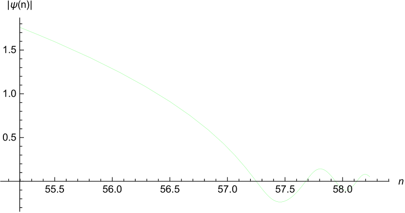
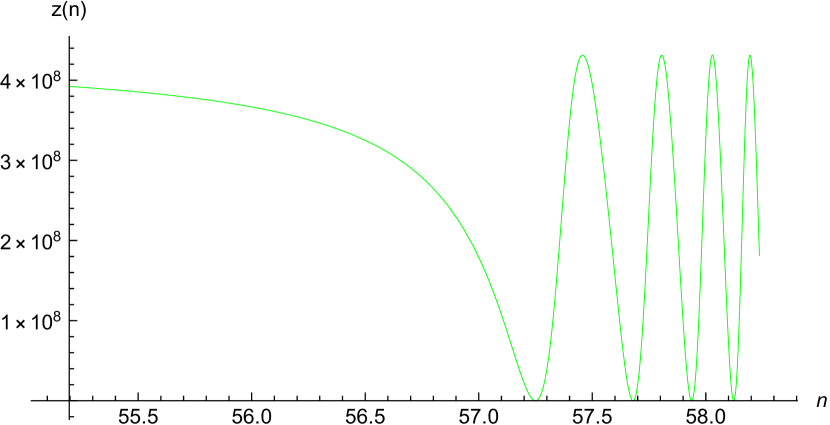
Figure 14: Plots of the dimensionless inflaton field $\psi(n)$ and the ratio $z\equiv q^{2}\psi^{2}/\chi^{2}$ after the end of inflation for the quadratic potential. Here we chose $q^{2}=\frac{1}{137}$.

The large field regime follows from the large argument expansion of the digamma function,

$$\psi(x)=\ln(x)-\frac{1}{2x}-\frac{1}{12x^{2}}+\frac{1}{120x^{4}}-\frac{1}{256x^{6}}+O\Bigl{(}\frac{1}{x^{8}}\Bigr{)}\;.$$ (164)

Substituting (164) in (162), and performing the various integrals gives,

$$\Delta V_{L}=\frac{H^{4}}{16\pi^{2}}\Biggl{\{}3z^{2}\ln\Bigl{(}\frac{2q^{2}\varphi\varphi^{*}}{s^{2}}\Bigr{)}\!-\!\frac{3}{2}z^{2}+\frac{Rz}{2H^{2}}\ln\Bigl{(}\frac{2q^{2}\varphi\varphi^{*}}{s^{2}}\Bigr{)}\!-\!(4\!+\!8\epsilon\!-\!3\epsilon^{2})z$$ (165)

$$\hskip 14.22636pt-\epsilon^{\prime}z-\Bigl{[}\frac{3}{4}\epsilon(1\!-\!\epsilon)(2\!-\!\epsilon)+\frac{7}{8}(1\!-\!\epsilon)\epsilon^{\prime}+\frac{1}{8}\epsilon^{\prime\prime}\Bigr{]}\ln^{2}(2z)+O\Bigl{(}\ln(z)\Bigr{)}\Biggr{\}}.\qquad$$

The leading contribution of (165) agrees with the famous flat space result of Coleman and Weinberg [2],

$$\Delta V\longrightarrow\frac{3(q^{2}\varphi\varphi^{*})^{2}}{16\pi^{2}}\ln\Bigl{(}\frac{2q^{2}\varphi\varphi^{*}}{s^{2}}\Bigr{)}\;.$$ (166)

The first three terms of (165) could be subtracted using allowed counterterms of the form $F(\varphi\varphi^{*},R)$ [9]. A prominent feature of the remaining terms is the presence of derivatives of the first slow roll parameter. These derivatives are typically very small during inflation but Figure 15 shows that they can be quite large after the end of inflation.

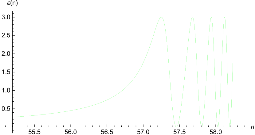
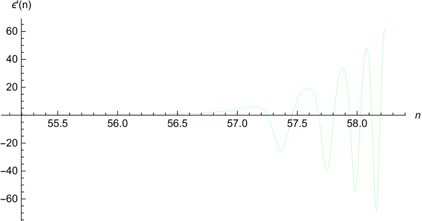
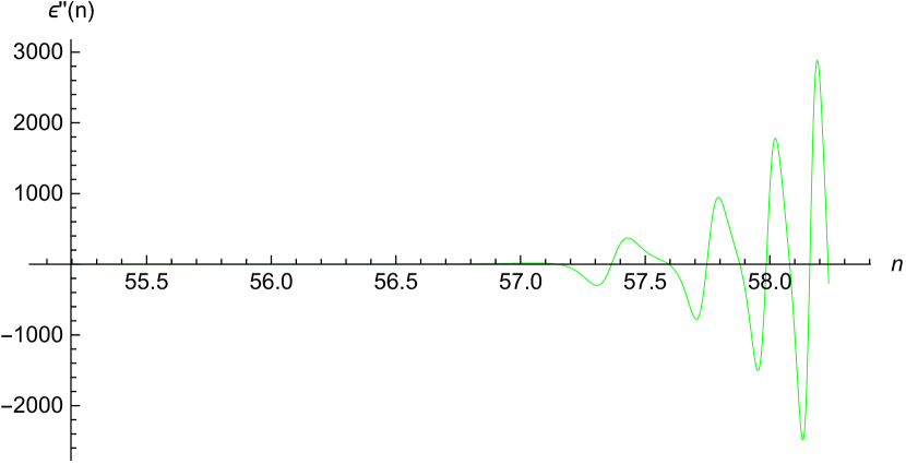
Figure 15: Plots of the first slow roll and its derivatives after the end of inflation for the quadratic potential.

The small field expansion derives from expanding the digamma functions in expression (162) in powers of $x$,

$$\psi\Bigl{(}\frac{1}{2}\!+\!\alpha(x)\Bigr{)} = \psi\Bigl{(}\frac{1}{1\!-\!\epsilon}\Bigr{)}-\psi^{\prime}\Bigl{(}\frac{1}{1\!-\!\epsilon}\Bigr{)}\frac{2x}{1\!-\!\epsilon^{2}}+O(x^{2})\;,$$ (167)

$$\psi\Bigl{(}\frac{1}{2}\!-\!\alpha(x)\Bigr{)} = \psi\Bigl{(}\frac{-\epsilon}{1\!-\!\epsilon}\Bigr{)}+\psi^{\prime}\Bigl{(}\frac{-\epsilon}{1\!-\!\epsilon}\Bigr{)}\frac{2x}{1\!-\!\epsilon^{2}}+O(x^{2})\;,$$ (168)

$$\psi\Bigl{(}\frac{1}{2}\!+\!\beta(x)\Bigr{)} = -\gamma-\frac{\pi^{2}}{6}\frac{2x}{(1\!-\!\epsilon)^{2}}+O(x^{2})\;,$$ (169)

$$\psi\Bigl{(}\frac{1}{2}\!-\!\beta(x)\Bigr{)} = -\frac{(1\!-\!\epsilon)^{2}}{2x}+1-\gamma+\Bigl{[}1\!+\!\frac{\pi^{2}}{6}\Bigr{]}\frac{2x}{(1\!-\!\epsilon)^{2}}+O(x^{2})\;.\qquad$$ (170)

The result is,

$$\Delta V_{L}=\frac{H^{4}}{16\pi^{2}}\Biggl{\{}\Biggl{[}\frac{R}{2H^{2}}\ln\Bigl{[}\frac{(1\!-\!\epsilon)^{2}H^{2}}{s^{2}}\Bigr{]}\!+\!1\!-\!8\epsilon\!+\!2\epsilon^{2}\!-\!2\epsilon^{\prime}-\frac{(6\epsilon^{\prime}\!+\!\epsilon^{\prime\prime})}{1\!-\!\epsilon}\!-\!\frac{{\epsilon^{\prime}}^{2}}{(1\!-\!\epsilon)^{2}}\Biggr{]}z$$ (171)

$$\hskip 56.9055pt+\frac{1}{2}\Bigl{[}(\partial_{n}\!+\!3\!-\!3\epsilon)(\partial_{n}\!+\!4\!-\!2\epsilon)\!-\!2\epsilon\Bigr{]}\Bigl{[}\psi\Bigl{(}\frac{1}{1\!-\!\epsilon}\Bigr{)}\!+\!\psi\Bigl{(}\frac{-\epsilon}{1\!-\!\epsilon}\Bigr{)}\Bigr{]}z$$

$$+\frac{1}{2}(\partial_{n}\!+\!3\!-\!3\epsilon)(\partial_{n}\!+\!4\!-\!2\epsilon)\Bigl{[}\psi^{\prime}\Bigl{(}\frac{1}{1\!-\!\epsilon}\Bigr{)}\!-\!\psi^{\prime}\Bigl{(}\frac{-\epsilon}{1\!-\!\epsilon}\Bigr{)}\Bigr{]}\frac{\epsilon z}{1\!-\!\epsilon^{2}}+O(z^{2})\Biggr{\}}.\qquad$$

Note that the $1/\epsilon$ pole from $\psi(\frac{-\epsilon}{1-\epsilon})$ on the penultimate line of (171) cancels against the double pole from $\psi^{\prime}(\frac{-\epsilon}{1-\epsilon})$ on the last line.

4.4 The Nonlocal Contribution

The nonlocal contribution to the effective potential is obtained by substituting the nonlocal contribution (148) to each coincident propagator in (140), and then into expression (6),

$$\Delta V^{\prime}_{\rm N}(\varphi\varphi^{*})=q^{2}N_{u}(n)+2q^{2}e^{-2n}N_{v}(n)$$ (172)

$$\hskip 113.81102pt+\frac{q^{2}H^{2}}{2M^{2}}\Bigl{(}\partial_{n}\!+\!3\!-\!\epsilon\Bigr{)}\Bigl{(}\partial_{n}\!+\!4\Bigr{)}\Bigl{[}N_{u}(n)\!-\!N_{u_{0}}(n)\Bigr{]}.\qquad$$

The nonlocal contributions to the various propagators are,

$$N_{u}(n) \!\!\!=\!\!\! \int_{0}^{\kappa_{n-4}}\!\!\frac{d\kappa\,\kappa^{2}}{32\pi^{3}G}\Biggl{[}e^{\mathcal{U}_{2,3}(n,\kappa,\mu)}-e^{\mathcal{U}_{1}(n,\kappa,\mu)}\Biggr{]},\qquad$$ (173)

$$N_{u_{0}}(n) \!\!\!=\!\!\! \int_{0}^{\kappa_{n-4}}\!\!\frac{d\kappa\,\kappa^{2}}{32\pi^{3}G}\Biggl{[}e^{\mathcal{U}_{2}(n,\kappa,0)}-e^{\mathcal{U}_{1}(n,\kappa,0)}\Biggr{]},\qquad$$ (174)

$$N_{v}(n) \!\!\!=\!\!\! \int_{0}^{\kappa_{n-4}}\!\!\frac{d\kappa\,\kappa^{2}}{32\pi^{3}G}\Biggl{[}e^{\mathcal{V}_{2,3}(n,\kappa,\mu)}-e^{\mathcal{V}_{1}(n,\kappa,\mu)}\Biggr{]}.\qquad$$ (175)

The nonlocal nature of these contributions derives from the integration over $\kappa$, which can be converted to an integration over $n_{\kappa}$,

$$\kappa\equiv e^{n_{\kappa}}\chi(n_{\kappa})\qquad\Longrightarrow\qquad\frac{d\kappa}{\kappa}=\Bigl{[}1\!-\!\epsilon(n_{\kappa})\Bigr{]}dn_{\kappa}\;.$$ (176)

After this is done, any factors of $\kappa$ depend on the earlier geometry.

A number of approximations result in huge simplification. First, note from Figures 4 and 5 that the ultraviolet approximation (114) for $\mathcal{U}(n,\kappa,\mu)$ is typically more negative than the late time approximations (123) and (124). Figures 8 and 9 show that the same rule applies to $\mathcal{V}(n,\kappa,\mu)$. Hence we can write,

$$N_{u}(n)\simeq\int_{0}^{\kappa_{n-4}}\!\!\frac{d\kappa\,\kappa^{2}}{16\pi^{3}G}\,e^{\mathcal{U}_{2,3}(n,\kappa,\mu)}\qquad,\qquad N_{v}(n)\simeq\int_{0}^{\kappa_{n-4}}\!\!\frac{d\kappa\,\kappa^{2}}{16\pi^{3}G}\,e^{\mathcal{V}_{2,3}(n,\kappa,\mu)}\;.$$ (177)

Second, because the temporal and transverse frequencies are nearly equal, we can write,

$$\omega^{2}_{u}(n,\mu)\simeq\omega^{2}_{v}(n,\mu)\qquad\Longrightarrow\qquad\mathcal{U}(n,\kappa,\mu)\simeq\mathcal{V}(n,\kappa,\mu)-2n\;.$$ (178)

When the mass vanishes there is so little difference between the ultraviolet approximation (114) and its late time extension (123) that we can ignore this contribution, $N_{u_{0}}(n)\simeq 0$. Next, Figures 6 and 10 imply that the late time approximations for $\mathcal{U}(n,\kappa,\mu)$ and $\mathcal{V}(n,\kappa,\mu)$ inherit their $\kappa$ dependence from the ultraviolet approximation at $n\simeq n_{\kappa}+4$, which is itself independent of $\mu$,

$$n>n_{\kappa}+4\qquad\Longrightarrow\qquad\mathcal{U}_{2,3}(n,\kappa,\mu)\simeq\mathcal{U}_{1}(n_{\kappa}\!+\!4,\kappa,0)+f_{2,3}(n,\mu)\;,$$ (179)

where $f_{2,3}(n,\mu)$ can be read off from expressions (123) and (124) by omitting the $\kappa$-dependent integration constants. Finally, we can use the slow roll form (112) for the amplitude reached after first horizon crossing and before the mass dominates,

$$e^{\mathcal{U}_{1}(n_{\kappa}+4,\kappa,0)}\simeq\frac{\chi^{2}(n_{\kappa})}{2\kappa^{3}}\times C\Bigl{(}\epsilon(n_{\kappa})\Bigr{)}\;.$$ (180)

Putting it all together gives,

$$\Delta V_{N}(\varphi\varphi^{*})\simeq 3q^{2}\!\!\int_{0}^{n-4}\!\!\!\!\!\!\!dn_{\kappa}\frac{[1\!-\!\epsilon(n_{\kappa})]\chi^{2}(n_{\kappa})C(n_{\kappa}))}{32\pi^{3}G}\times e^{f_{2,3}(n,\mu)}$$ (181)

$$+\frac{q^{2}\chi^{2}(n)}{2\mu^{2}}(\partial_{n}\!+\!3\!-\!\epsilon)(\partial_{n}\!+\!4)\!\!\int_{0}^{n-4}\!\!\!\!\!\!dn_{\kappa}\frac{[1\!-\!\epsilon(n_{\kappa})]\chi^{2}(n_{\kappa})C(\epsilon(n_{\kappa}))}{32\pi^{3}G}\!\times\!e^{f_{2,3}(n,\mu)}\!.\qquad$$

5 Conclusions

In section 2 we derived an exact, dimensionally regulated, Fourier mode sum (50) for the Lorentz gauge propagator of a massive photon on an arbitrary cosmological background (3). Our result is expressed in terms of mode functions $t(\eta,k)$, $u(\eta,k,M)$ and $v(\eta,k,M)$ whose defining relations are (10), (24) and (22), which respectively represent massless minimally coupled scalars, massive temporal photons, and massive spatially transverse photons. The photon propagator can also be expressed as a sum (51) of bi-vector differential operators acting on the scalar propagators $i\Delta_{t}(x;x^{\prime})$, $i\Delta_{u}(x;x^{\prime})$ and $i\Delta_{v}(x;x^{\prime})$ associated with the three mode functions. Because Lorentz gauge is an exact gauge there should be no linearization instability, even on de Sitter, such as occurs for Feynman gauge [30, 31].

In section 3 we converted to a dimensionless form with time represented by the number of e-foldings $n$ since the beginning of inflation, and the wave number, mass and Hubble parameter all expressed in reduced Planck units, $\kappa\equiv\sqrt{8\pi G}\,k$, $\mu\equiv\sqrt{8\pi G}\,M$ and $\chi(n)\equiv\sqrt{8\pi G}\,H(\eta)$. Analytic approximations were derived for the amplitudes $\mathcal{T}(n,\kappa)$, $\mathcal{U}(n,\kappa,\mu)$ and $\mathcal{V}(n,\kappa,\mu)$ associated with each of the mode functions. Which approximation to use is controlled by first horizon crossing at $\kappa=e^{n_{\kappa}}\chi(n_{\kappa})$ and mass domination at $\mu=\frac{1}{2}\chi(n_{\mu})$. Until shortly after first horizon crossing we employ the ultraviolet approximations (109), (114) and (126). After first horizon crossing and before mass domination the appropriate approximations are (112), (123) and (131). And after mass domination (which $\mathcal{T}(n,\kappa)$ never experiences) the amplitudes are well approximated by (124) and (132). The validity of these approximations was checked against explicit numerical solutions for inflation driven by the simple quadratic model, and by the phenomenologically favored plateau model (133).

In section 4 we applied our approximations to compute the effective potential induced by photons coupled to a charged inflaton. Our result consists of a part (162) which depends locally on the geometry (3) and a numerically smaller part (181) which depends on the past history. The local part was expanded both for the case of large field strength (165), and for small field strength (171). The existence of the second, nonlocal contribution, was conjectured on the basis of indirect arguments [5] that have now been explicitly confirmed. Another conjecture that has been confirmed is the rough validity of extrapolating de Sitter results [1, 6] from the constant Hubble parameter of de Sitter background to the time dependent one of a general cosmological background (3). However, we now have good approximations for the dependence on the first slow roll parameter $\epsilon(n)$.

We have throughout considered the inflaton field in the vector mass $M^{2}\equiv 2q^{2}\varphi\varphi^{*}$ to be constant because this is how the “effective potential” is defined. It would be easy to relax this assumption with only minor changes in the result. In particular, equations (6) and (140) would still pertain. Our approximations for the propagators would remain, so that renormalization would be unaffected. The only thing that would change is that the $\partial_{n}$ derivatives in expression (140) would now act on $\psi$ as well as $\epsilon$ and $\chi$. This would produce some factors of $\epsilon$ and its first derivative through the relation,

$$\psi^{\prime}{\psi^{\prime}}^{*}=\frac{1}{2}(D\!-\!2)\epsilon\;.$$ (182)

Our most important result is probably the fact that electromagnetic corrections to the effective potential depend upon first and second derivatives of the first slow roll parameter. One consequence is that the effective potential from electromagnetism responds more strongly to changes in the geometry than for scalars [26] or spin one half fermions [32]. This can be very important during reheating (see Figure 15); it might also be significant if features occur during inflation. Another consequence is that there cannot be perfect cancellation between the positive effective potentials induced by bosons and the negative potentials induced by fermions [10]. Note that the derivatives of $\epsilon$ come exclusively from the constrained part of the photon propagator — the $t(\eta,k)$ and $u(\eta,k)$ modes — which is responsible for long range electromagnetic interactions. Dynamical photons — the $v(\eta,k)$ modes — produce no derivatives at all. These statements can be seen from expression (140), which is exact, independent of any approximation.

We close with a speculation based on the correlation between the spin of the field and the number of derivatives it induces in the effective potential: scalars produce no derivatives [26], spin one half fermions induce one derivative [32], and this paper has shown that spin one vectors give two derivatives. It would be interesting to see if the progression continues for gravitinos (which ought to induce three derivatives) and gravitons (which would induce four derivatives). Of course gravitons do not acquire a mass through coupling to a scalar inflaton, but they do respond to it, and the mode equations have been derived in a simple gauge [33, 34]. Until now it was not possible to do much with this system because it can only be solved exactly for the case of constant $\epsilon(n)$, however, we now have a reliable approximation scheme that can be used for arbitrary $\epsilon(n)$. Further, we have a worthy object of study in the graviton 1-point function, which defines how quantum 0-point fluctuations back-react to change the classical geometry. At one loop order it consists of the same sort of coincident propagator we have studied in this paper. On de Sitter background the result is just a constant times the de Sitter metric [35], which must be absorbed into a renormalization of the cosmological constant if “$H$” is to represent the true Hubble parameter. Now suppose that the graviton propagator for general first slow roll parameter consists of a local part with up to 4th derivatives of $\epsilon(n)$ plus a nonlocal part. That sort of result could not be absorbed into any counterterm. So perhaps there is one loop back-reaction after all [36], and de Sitter represents a case of unstable equilibrium?

Acknowledgements

This work was partially supported by Taiwan MOST grants 108-2112-M-006-004 and 107-2119-M-006-014; by NSF grants PHY-1806218 and PHY-1912484; and by the Institute for Fundamental Theory at the University of Florida.

References

- [1] B. Allen, Nucl. Phys. B 226, 228-252 (1983) doi:10.1016/0550-3213(83)90470-4
- [2] S. R. Coleman and E. J. Weinberg, Phys. Rev. D 7, 1888-1910 (1973) doi:10.1103/PhysRevD.7.1888
- [3] Y. Akrami et al. [Planck], Astron. Astrophys. 641, A10 (2020) doi:10.1051/0004-6361/201833887 [arXiv:1807.06211 [astro-ph.CO]].
- [4] D. R. Green, Phys. Rev. D 76, 103504 (2007) doi:10.1103/PhysRevD.76.103504 [arXiv:0707.3832 [hep-th]].
- [5] S. P. Miao and R. P. Woodard, JCAP 09, 022 (2015) doi:10.1088/1475-7516/2015/9/022 [arXiv:1506.07306 [astro-ph.CO]].
- [6] T. Prokopec, N. C. Tsamis and R. P. Woodard, Annals Phys. 323, 1324-1360 (2008) doi:10.1016/j.aop.2007.08.008 [arXiv:0707.0847 [gr-qc]].
- [7] S. P. Miao, S. Park and R. P. Woodard, Phys. Rev. D 100, no.10, 103503 (2019) doi:10.1103/PhysRevD.100.103503 [arXiv:1908.05558 [gr-qc]].
- [8] J. H. Liao, S. P. Miao and R. P. Woodard, Phys. Rev. D 99, no.10, 103522 (2019) doi:10.1103/PhysRevD.99.103522 [arXiv:1806.02533 [gr-qc]].
- [9] R. P. Woodard, Lect. Notes Phys. 720, 403-433 (2007) doi:10.1007/978-3-540-71013-4_14 [arXiv:astro-ph/0601672 [astro-ph]].
- [10] S. P. Miao, L. Tan and R. P. Woodard, Class. Quant. Grav. 37, no.16, 165007 (2020) doi:10.1088/1361-6382/ab9881 [arXiv:2003.03752 [gr-qc]].
- [11] N. C. Tsamis and R. P. Woodard, J. Math. Phys. 48, 052306 (2007) doi:10.1063/1.2738361 [arXiv:gr-qc/0608069 [gr-qc]].
- [12] N. Aghanim et al. [Planck], Astron. Astrophys. 641, A6 (2020) doi:10.1051/0004-6361/201833910 [arXiv:1807.06209 [astro-ph.CO]].
- [13] A. A. Starobinsky, Adv. Ser. Astrophys. Cosmol. 3, 130-133 (1987) doi:10.1016/0370-2693(80)90670-X
- [14] T. M. Janssen, S. P. Miao, T. Prokopec and R. P. Woodard, Class. Quant. Grav. 25, 245013 (2008) doi:10.1088/0264-9381/25/24/245013 [arXiv:0808.2449 [gr-qc]].
- [15] S. P. Miao, N. C. Tsamis and R. P. Woodard, J. Math. Phys. 52, 122301 (2011) doi:10.1063/1.3664760 [arXiv:1106.0925 [gr-qc]].
- [16] A. Vilenkin and L. H. Ford, Phys. Rev. D 26, 1231 (1982) doi:10.1103/PhysRevD.26.1231
- [17] A. D. Linde, Phys. Lett. B 116, 335-339 (1982) doi:10.1016/0370-2693(82)90293-3
- [18] A. A. Starobinsky, Phys. Lett. B 117, 175-178 (1982) doi:10.1016/0370-2693(82)90541-X
- [19] V. K. Onemli and R. P. Woodard, Class. Quant. Grav. 19, 4607 (2002) doi:10.1088/0264-9381/19/17/311 [arXiv:gr-qc/0204065 [gr-qc]].
- [20] V. K. Onemli and R. P. Woodard, Phys. Rev. D 70, 107301 (2004) doi:10.1103/PhysRevD.70.107301 [arXiv:gr-qc/0406098 [gr-qc]].
- [21] S. P. Miao, N. C. Tsamis and R. P. Woodard, J. Math. Phys. 50, 122502 (2009) doi:10.1063/1.3266179 [arXiv:0907.4930 [gr-qc]].
- [22] M. G. Romania, N. C. Tsamis and R. P. Woodard, Class. Quant. Grav. 30, 025004 (2013) doi:10.1088/0264-9381/30/2/025004 [arXiv:1108.1696 [gr-qc]].
- [23] M. G. Romania, N. C. Tsamis and R. P. Woodard, JCAP 08, 029 (2012) doi:10.1088/1475-7516/2012/08/029 [arXiv:1207.3227 [astro-ph.CO]].
- [24] D. J. Brooker, N. C. Tsamis and R. P. Woodard, Phys. Rev. D 93, no.4, 043503 (2016) doi:10.1103/PhysRevD.93.043503 [arXiv:1507.07452 [astro-ph.CO]].
- [25] D. J. Brooker, N. C. Tsamis and R. P. Woodard, Phys. Rev. D 96, no.10, 103531 (2017) doi:10.1103/PhysRevD.96.103531 [arXiv:1708.03253 [gr-qc]].
- [26] A. Kyriazis, S. P. Miao, N. C. Tsamis and R. P. Woodard, Phys. Rev. D 102, no.2, 025024 (2020) doi:10.1103/PhysRevD.102.025024 [arXiv:1908.03814 [gr-qc]].
- [27] T. M. Janssen, S. P. Miao, T. Prokopec and R. P. Woodard, JCAP 05, 003 (2009) doi:10.1088/1475-7516/2009/05/003 [arXiv:0904.1151 [gr-qc]].
- [28] D. J. Brooker, S. D. Odintsov and R. P. Woodard, Nucl. Phys. B 911, 318-337 (2016) doi:10.1016/j.nuclphysb.2016.08.010 [arXiv:1606.05879 [gr-qc]].
- [29] I. S. Gradshteyn and I. M. Ryzhik, “Table of Integrals, Series and Products, 4th Edition,” (New York, Academic Press, 1965).
- [30] E. O. Kahya and R. P. Woodard, Phys. Rev. D 72, 104001 (2005) doi:10.1103/PhysRevD.72.104001 [arXiv:gr-qc/0508015 [gr-qc]].
- [31] E. O. Kahya and R. P. Woodard, Phys. Rev. D 74, 084012 (2006) doi:10.1103/PhysRevD.74.084012 [arXiv:gr-qc/0608049 [gr-qc]].
- [32] A. Sivasankaran and R. P. Woodard, [arXiv:2007.11567 [gr-qc]].
- [33] J. Iliopoulos, T. N. Tomaras, N. C. Tsamis and R. P. Woodard, Nucl. Phys. B 534, 419-446 (1998) doi:10.1016/S0550-3213(98)00528-8 [arXiv:gr-qc/9801028 [gr-qc]].
- [34] L. R. Abramo and R. P. Woodard, Phys. Rev. D 65, 063515 (2002) doi:10.1103/PhysRevD.65.063515 [arXiv:astro-ph/0109272 [astro-ph]].
- [35] N. C. Tsamis and R. P. Woodard, Annals Phys. 321, 875-893 (2006) doi:10.1016/j.aop.2005.08.004 [arXiv:gr-qc/0506056 [gr-qc]].
- [36] G. Geshnizjani and R. Brandenberger, Phys. Rev. D 66, 123507 (2002) doi:10.1103/PhysRevD.66.123507 [arXiv:gr-qc/0204074 [gr-qc]].