Effect of low-level jet height on wind farm performance

Abstract

Low-level jets (LLJs) are the wind maxima in the lowest 50 to 1000 m of atmospheric boundary layers. Due to their significant influence on the power production of wind farms it is crucial to understand the interaction between LLJs and wind farms. In the presence of a LLJ, there are positive and negative shear regions in the velocity profile. The positive shear regions of LLJs are continuously turbulent, while the negative shear regions have limited turbulence. We present large eddy simulations of wind farms in which the LLJ is above, below, or in the middle of the turbine rotor swept area. We find that the wakes recover relatively fast when the LLJ is above the turbines. This is due to the high turbulence below the LLJ and the downward vertical entrainment created by the momentum deficit due to the wind farm power production. This harvests the jet’s energy and aids wake recovery. However, when the LLJ is below the turbine rotor swept area, the wake recovery is very slow due to the low atmospheric turbulence above the LLJ. The energy budget analysis reveals that the entrainment fluxes are maximum and minimum when the LLJ is above and in the middle of the turbine rotor swept area, respectively. Surprisingly, we find that the negative shear creates a significant entrainment flux upward when the LLJ is below the turbine rotor swept area. This facilitates energy extraction from the jet, which is beneficial for the performance of downwind turbines.

I Introduction

A low-level jet (LLJ) is the maximum in the wind velocity profile in the atmospheric boundary layer (ABL). When the wind in the residual layerBrutsaert (1982) is decoupled from the surface friction and subjected to inertial oscillations, the flow in the residual layer accelerates to super-geostrophic magnitudes and forms a LLJ Blackadar (1957). These jets are observed in the lowest 50 to 1000 m of the ABL (Smedman, Högström, and Bergström, 1996) and are most pronounced in weak to moderately stable ABLs Baas et al. (2009); Banta (2008). Figure 1 shows a sketch of the velocity, potential temperature, and turbulence flux profiles in a stable ABL. LLJs Kelley et al. (2004); Banta et al. (2002); Smedman, Tjernström, and Högström (1993) have been reported all over the world with frequent occurrences in India Prabha et al. (2011), China Liu et al. (2014), the Great Plains of the United States Arritt et al. (1997) and the North Sea region of Europe Kalverla et al. (2019); Wagner et al. (2019). Field observations show that in the IJmuiden region of North Sea, LLJs are observed with a frequency of 7.56% in summer and 6.61% in springDuncan (2018); Kalverla et al. (2017). LLJs in the North Sea are associated with shallow boundary-layer heights Duncan (2018); Baas et al. (2009), i.e. these jets can influence the wind farm power production. It has been reported that LLJs can increase the capacity factors by 60% under nocturnal conditions Wilczak et al. (2015), and measurements in Western OklahomaGreene et al. (2009) indicate that LLJs increase the power production compared to the case without jets. As a result, the importance, relevance, and urgency of research into LLJ for wind farm applications have been outlined by van Kuik et al. van Kuik et al. (2016) in their long term European Research Agenda and a recent review by Porté-Agel et al. Porté-Agel, Bastankhah, and Shamsoddin (2020).
It is well established in the wind energy community that LLJs affect the performance of wind turbines Sisterson and Frenzen (1978). Below the jet height ($z_{\text{jet}}$) the velocity profile has a positive shear, and above the jet height there is a negative shear. The top panel of Fig. 1 shows a turbine with hub-height ($z_{h}$) lower than the jet height, i.e. $z_{\text{jet}}>z_{h}$, operating in the positive shear region. The bottom panel shows a turbine with the hub-height higher than the jet height, i.e. $z_{\text{jet}}<z_{h}$, operating in the negative shear region. The potential temperature profile shows significant surface inversion with a residual layer above. Above the surface inversion the boundary layer has negligible turbulence and the region is associated with the negative shear, see Fig. 1.
As noted above, LLJs generally form at the top of stable surface inversions Baas et al. (2009), above which the turbulence is negligible Blackadar (1957). During an LLJ event, the turbulence intensity and turbulence kinetic energy are lower than for unstable conditions Gutierrez et al. (2016). The effect of LLJs on wind turbine and wind farm performance has been studied before. Lu & Porté-Agel Lu and Porté-Agel (2011) performed large eddy simulations (LES) of an ‘infinite’ wind farm in the stable boundary layer, and they report the formation of non-axisymmetric wakes and a decrease in the LLJ strength due to the energy extraction by the turbines. LLJ elimination due to wind turbine momentum extraction has also been reported in similar LES studies Abkar, Sharifi, and Porté-Agel (2016); Bhaganagar and Debnath (2015); Sharma, Parlange, and Calaf (2017); Ali et al. (2017). Also, mesoscale simulations in which wind farms are modeled as localized roughness elements show that LLJs are eliminated by wind farmsFitch, Olson, and Lundquist (2013). Furthermore, due to the velocity maximum and strong shear, both the power production and the fatigue loads on wind turbines are affected by the LLJ Gutierrez et al. (2017).

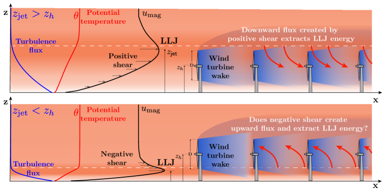
Figure 1: Problem definition. The top figure shows turbines operating in positive shear when the LLJ is above the turbine rotor swept area ($z_{\mathsf{jet}}>z_{h}$). The bottom figure shows turbines operating in negative shear when the LLJ is below the turbine rotor swept area ($z_{\mathsf{jet}}<z_{h}$). We study whether the negative shear increases the energy extraction from the jet by creating an upward flux. The figure also shows that the turbulent momentum flux is negligible above the LLJ. The potential temperature $\theta$ profile reveals that the boundary layer is stably stratified and shows a residual layer with a constant temperature above the LLJ.

In a fully developed wind farm boundary layer, the power production depends on the vertical entrainment fluxes from above, which is created by the momentum deficit inside the wind farm. Wind turbines operating below the LLJ are subjected to positive shear and continuous turbulence. In that case, the downward entrainment fluxes are enhanced due to which the energy of the LLJ is harvested Lu and Porté-Agel (2011); Na et al. (2018); Gadde and Stevens (2020). Recently, Doosttalab et al.Doosttalab et al. (2020) conducted experiments in which they studied the interaction between a wind farm and a synthetic jet, they report that entrainment fluxes are enhanced due to the shear layer associated with the LLJ. However, situations might arise when the turbines have to operate in the negative shear region with reduced turbulence. Aeroelastic simulations of the interaction between a LLJ and a wind turbine show that the loading on a wind turbine decreases when it operates in the jet’s negative shear region. Based on these simulations, Gutierrez et al. Gutierrez et al. (2016) suggest installing turbines at heights where negative shear occurs. However, the region where negative shear occurs is also a region of reduced turbulence, which negatively affects wake recovery and hence the power production of downwind turbines. Stevens and Meneveau (2017); Porté-Agel, Bastankhah, and Shamsoddin (2020); Ali et al. (2018)
Previous studies have mostly focused on wind turbines and wind farms operating in the jet’s positive shear region. The presence of negative shear and negligible turbulence above the LLJ leads to scenarios in which the wind farm and LLJ interaction is not straightforward. As mentioned before, when the LLJ is above the turbines, the momentum deficit creates a downward entrainment flux, which facilitates the extraction of LLJ’s energy, see the top schematic in Fig. 1. However, it is not yet explored if the negative shear creates an upward entrainment flux when the LLJ is below the turbine rotor swept area, see the bottom schematic in Fig. 1. Therefore, the objective of the study is to understand how changing the LLJ height relative to the turbine hub-height affects wake recovery and power production of downstream turbines. This can be done in two ways: by keeping the jet height constant and changing the turbine height or simulating jets of different heights which involves multiple spin-up simulations with different boundary layer properties. Changing jet height is complicated and computationally expensive, therefore we follow the easiest and the most straightforward way of changing the ratio $z_{\text{jet}}<z_{h}$ by changing the turbine height. In this work, we consider three different scenarios:

• the LLJ above the turbine rotor swept area, i.e. $z_{\text{jet}}<z_{h}$.

• the LLJ in the middle of the turbine rotor swept area, i.e. $z_{\text{jet}}\approx z_{h}$.

• the LLJ below the turbine rotor swept area, i.e. $z_{\text{jet}}>z_{h}$.

In section II, the simulation methodology and the wind farm configuration are described. In section III the main observations are discussed and in section IV the major conclusions are detailed.

II Simulation methodology

II.1 Governing equations

We numerically integrate the filtered Navier-Stokes equation coupled with the Boussinesq approximation to model buoyancy. The governing equations are:

$$\partial_{\mathit{i}}\widetilde{u}_{\mathit{i}} =0,$$ (1)

$$\begin{split}\partial_{\mathit{t}}\widetilde{u}_{\mathit{i}}+\partial_{\mathit{j}}\left(\widetilde{u}_{\mathit{i}}\widetilde{u}_{\mathit{j}}\right)&=-\partial_{\mathit{i}}\widetilde{p}-\partial_{\mathit{j}}\tau_{\mathit{ij}}+g\beta(\widetilde{\theta}-\widetilde{\theta}_{\mathit{0}})\delta_{\mathit{i3}}\\ &+f_{c}(U_{g}-\widetilde{u})\delta_{i2}-f_{c}(V_{g}-\widetilde{v})\delta_{i1}+\widetilde{f}_{x}\delta_{i1}+\widetilde{f}_{y}\delta_{i2},\end{split}$$ (2)

$$\partial_{\mathit{t}}\widetilde{\theta}+\widetilde{u}_{\mathit{j}}\partial_{\mathit{j}}\widetilde{\theta} =-\partial_{\mathit{j}}q_{\mathit{j}},$$ (3)

here the tilde represents a spectral cut-off filter of size $\Delta$, $\widetilde{u}_{\mathit{i}}=\left(\widetilde{u},\widetilde{v},\widetilde{w}\right)$ and $\widetilde{\theta}$ are the filtered velocity and potential temperature, respectively, $g$ is the gravitational acceleration, $\beta=1/\theta_{\mathit{0}}$ is the buoyancy parameter with respect to the reference potential temperature $\theta_{\mathit{0}}$, $\delta_{\mathit{ij}}$ is the Kronecker delta, and $f_{c}$ is the Coriolis parameter. The ABL is forced by a mean pressure $p_{\infty}$, represented by the geostrophic wind with the relation, $U_{g}=-\frac{1}{{\rho}f_{c}}\frac{\partial{p_{\infty}}}{\partial{y}}$ and $V_{g}=\frac{1}{{\rho}f_{c}}\frac{\partial{p_{\infty}}}{\partial{x}}$ as its components. $\widetilde{p}=\widetilde{p}^{*}/\rho+\sigma_{kk}/3$ is the modified pressure, which is the sum of the trace of the SGS stress, $\sigma_{kk}/3$, and the kinematic pressure $\widetilde{p}^{*}/\rho$, where $\rho$ is the density of the fluid.

It is well established that the actuator disk model can capture the wake dynamics starting from $1$ to $2$ diameters downstream of the turbine sufficiently accurately Stevens and Meneveau (2017); Stevens, Martínez-Tossas, and Meneveau (2018); Wu and Porté-Agel (2011). Therefore, the actuator disk model can be used to study the large scale flow phenomena in a wind farm on which we focus here. We note that the actuator disk model cannot capture the vortex structures near the turbine due to the absence of the turbine bladesSørensen (2011); Troldborg, Sørensen, and Mikkelsen (2010); Stevens and Meneveau (2017). To capture vortex structures very high resolution actuator line model simulations are required, which is not feasible for large wind farms Stevens, Martínez-Tossas, and Meneveau (2018). Therefore, we use a well-validated actuator disk model Jimenez et al. (2007, 2008); Calaf, Meneveau, and Meyers (2010); Stevens, Graham, and Meneveau (2014); Stevens, Gayme, and Meneveau (2016); Zhang, Arendshorst, and Stevens (2019); Gadde and Stevens (2019) in this study. The turbine forces $\widetilde{f}_{x}$ and $\widetilde{f}_{y}$ in equation (2) are modeled using the turbine force

$$F_{t}=-\frac{1}{2}\rho{C_{T}}{U^{2}_{\infty}}\frac{\pi}{4}D^{2},$$ (4)

where $C_{T}$ is the thrust coefficient and $U_{\infty}$ is the upstream undisturbed reference velocity. Equation (4) is only applicable for isolated turbines Jimenez et al. (2007, 2008). In wind farm simulations the upstream velocity $U_{\infty}$ cannot be readily specified. Consequently, it is common practice Calaf, Meneveau, and Meyers (2010); Calaf, Parlange, and Meneveau (2011) to use actuator disk theory to relate $U_{\infty}$ with the rotor disk velocity $U_{d}$,

$$U_{\infty}=\frac{U_{d}}{\left(1-a\right)}$$ (5)

where $a$ is the axial induction factor. The turbine forces are calculated by substituting equation (5) in equation (4). For a detailed description and validation of the employed actuator disk model we refer the reader to Refs. Calaf, Meneveau, and Meyers (2010); Calaf, Parlange, and Meneveau (2011); Stevens, Martínez-Tossas, and Meneveau (2018).

The terms involving molecular viscosity are neglected due to the high Reynolds number of the ABL flow. $\tau_{\mathit{ij}}=\widetilde{u_{\mathit{i}}u_{\mathit{j}}}-\widetilde{u}_{\mathit{i}}\widetilde{u}_{\mathit{j}}$ is the traceless part of the SGS stress tensor and $q_{\mathit{j}}=\widetilde{u_{\mathit{j}}\theta}-\widetilde{u}_{\mathit{j}}\widetilde{\theta}$ is the SGS heat flux tensor. The SGS stresses and heat fluxes are modeled as,

$$\tau_{\mathit{ij}} =\widetilde{u_{\mathit{i}}u_{\mathit{j}}}-\widetilde{u}_{\mathit{i}}\widetilde{u}_{\mathit{j}}=-2\nu_{T}\widetilde{S}_{ij}=-2(C_{s}\Delta)^{2}|\widetilde{S}|\widetilde{S}_{ij},$$ (6)

$$q_{\mathit{j}} =\widetilde{u_{\mathit{j}}\theta}~{}~{}-\widetilde{u}_{\mathit{j}}\widetilde{\theta}~{}~{}=-\nu_{\theta}\partial_{j}\widetilde{\theta}~{}~{}=-(D_{s}\Delta)^{2}|\widetilde{S}|\partial_{j}\widetilde{\theta},$$ (7)

where $\widetilde{S}_{ij}=\frac{1}{2}\left(\partial_{j}{\widetilde{u}_{i}}+\partial_{i}{\widetilde{u}_{j}}\right)$ is the grid-scale strain rate tensor, $\nu_{T}$ is the eddy viscosity, $C_{s}$ is the Smagorinsky coefficient for the SGS stresses, $\Delta$ is the grid size, $\nu_{\theta}$ is the eddy heat diffusivity, $D_{s}$ is the Smagorinsky coefficient for the SGS heat flux, and $|\widetilde{S}|=\sqrt{2\widetilde{S}_{ij}\widetilde{S}_{ij}}$. To model the SGS stresses without any ad-hoc modifications, we use a tuning-free, scale-dependent, dynamic model based on the Lagrangian averaging of the coefficients Bou-Zeid, Meneveau, and Parlange (2005); Stoll and Porté-Agel (2006, 2008). The model has been found to be highly suitable for inhomogeneous flows such as the flow inside wind farmsStevens, Gayme, and Meneveau (2016). For further details and validation of the code we refer to Gadde et al. (2020) Gadde, Stieren, and Stevens (2020).

II.2 Numerical method

We use a standard pseudo-spectral method to calculate the derivatives in horizontal directions and a second-order central difference scheme to calculate the gradients in the vertical direction. A second-order Adams-Bashforth scheme is employed to advance the solution in time. The aliasing errors in the non-linear terms are removed by the 3/2 anti-aliasing methodCanuto et al. (1988). The advective terms in the governing equations are written in the rotational formFerziger and Perić (2002). We discretize the horizontal directions uniformly with $n_{x}$, $n_{y}$, grid points in the streamwise and spanwise directions, respectively. This results in grid sizes of $\Delta_{x}=L_{x}/n_{x}$, $\Delta_{y}=L_{y}/n_{y}$ in the horizontal directions. In the vertical direction, we use a uniform grid up to a certain height, above which we use a stretched grid. The vertical grid size in the uniform region of the computational domain is represented by $\Delta_{z}$. The horizontal and vertical computational planes are staggered, such that for the horizontal velocity components, the first vertical grid point above the ground is located at $\Delta_{z}/2$. No-slip and free-slip boundary conditions are imposed at the lowest and the topmost computational plane, respectively. We use the Monin-Obukhov similarity theory Moeng (1984) to model the instantaneous stress and heat flux at the wall by using the velocity and temperature at the first grid point above the wall

$$\tau_{i3|w}=-{u_{*}^{2}}\frac{\widetilde{u}_{i}}{\widetilde{u}_{r}}=-\Bigg{(}\frac{\widetilde{u}_{r}\kappa}{\text{ln}(\Delta{z}/2z_{o})-\psi_{M}}\Bigg{)}^{2}\frac{\widetilde{u}_{i}}{\widetilde{u}_{r}},$$ (8)

and

$$q_{*} =\frac{u_{*}\kappa(\theta_{s}-\widetilde{\theta})}{\text{ln}(\Delta{z}/2z_{os})-\psi_{H}}.$$ (9)

In the above equations, $\widetilde{u}_{i}$ and $\widetilde{\theta}$ represent the filtered grid-scale velocities and potential temperature at the first grid point above the ground, $u_{*}$ is the frictional velocity, $z_{o}$ is the roughness height for momentum, $z_{os}$ is the roughness height for heat flux, $\kappa=0.4$ is the von Kármán constant, $\widetilde{u}_{r}=\sqrt{\widetilde{u}^{2}+\widetilde{v}^{2}}$ is the resolved velocity magnitude, and $\theta_{s}$ is the grid scale potential temperature at the surface. $\psi_{M}$ and $\psi_{H}$ are the stability corrections for momentum and heat flux, respectively. We use the stability correction used by Beare et al. Beare et al. (2006) to simulate the stable boundary layer, i.e. $\psi_{M}=-4.8z/L$ and $\psi_{H}=-7.8z/L$, where $L=-({u_{*}}^{3}\theta_{0})/({\kappa}gq_{*})$ is the surface Obukhov length. We note that, for convenience, the tildes representing filtered LES quantities are omitted in the remainder of the paper.

II.3 Boundary layer characteristics

Table 1: The table gives the size of the computational domain and the used grid resolution in the streamwise ($n_{x}$), spanwise ($n_{y}$), and vertical ($n_{z}$) direction, respectively. $C_{r}$ is the surface cooling rate, $z_{i}$ is the boundary layer height, $z_{\text{jet}}$ is the jet height, $u_{*}$ is the friction velocity, $u_{\text{jet}}/G$ is the non-dimensionalized jet velocity, and $z_{i}/L$ represents the stability parameter.

Domain size	$n_{x}\times n_{y}\times n_{z}$	$C_{r}$ [$\text{K}\cdot\text{h}^{-1}$]	$z_{i}$ [m]	$z_{\text{jet}}$ [m]	$u_{*}$ [m$\text{s}^{-1}$]	$u_{\text{jet}}/G$	$z_{i}/L$
$11.52$ km $\times$ $4.6$ km $\times$ $3.84$ km	$1280\times 512\times 384$	0.50	131.6	125	0.192	1.21	2.95

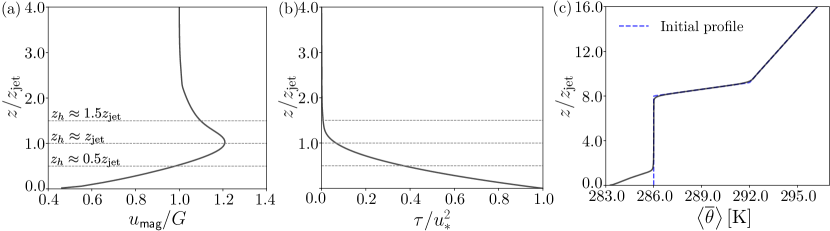
Figure 2: (a) Horizontally averaged wind magnitude $u_{\text{mag}}/G$, (b) the vertical momentum flux, and (c) the temperature profiles plotted as a function of the height. Height is normalized with the jet height.

We consider a continuously turbulent, moderately stable ABL with a capping inversion at approximately 1000 m. The temperature profile is slightly modified form of the one used in the LES of second Global Earth and Water Cycle Experiment (GEWEX) ABL study (GABLS-2) single column intercomparison setup Kumar et al. (2010). The boundary layer is initialized with a constant temperature of 286 K below 1000 m, a capping inversion of strength 6 K between 1000 m and 1150 m, followed by a constant temperature gradient of 5 $\text{K}\cdot\text{km}^{-1}$ above. The initial temperature profile is shown by the blue dashed lines in Fig. 2(c). The roughness height is, $z_{o}=0.002$ m for momentum corresponding to offshore conditions Dörenkämper et al. (2015) and $z_{os}=\frac{z_{o}}{10}=0.0002$ m Brutsaert (1982) for modelling the heat flux. The surface is cooled at a constant rate of 0.5 $\text{K}\cdot\text{hour}^{-1}$. The geostrophic forcing is set to $G=(U_{g},V_{g})=(8.0,0.0)$ $\text{m}\text{s}^{-1}$ and the Coriolis parameter is set to $f_{c}=1.159\times 10^{-4}$ $\text{s}^{-1}$ corresponding to a latitude of $52.8^{\circ}$, which is representative for the Dutch North Sea. The velocity is initialized with the geostrophic velocity, and uniform random perturbations are added to the initial velocities and temperature up to a height of 500 m to trigger turbulence. We note that the boundary layer reaches a quasi-steady state at the end of 8${}^{\text{th}}$ hour.
The boundary layer characteristics relevant to this study are given in table 1. The jet height $z_{\text{jet}}$ is approximately $125$ m. The boundary layer height, defined as the height where the shear stress reaches 5% of its surface valueBeare et al. (2006), is 131.6 m. The ratio of boundary layer height to the surface Obukhov length is $z_{i}/L=2.95$. Scaling regimes reported by Holtslag and Nieuwstadt Holtslag and Nieuwstadt (1986) show that for $z_{i}/L<3$, stable boundary layers show negligible intermittency throughout the boundary layer. This confirms that the boundary layer is moderately stable Holtslag and Nieuwstadt (1986). The jet velocity is 9.68 m/s. It is worth mentioning here that LLJs with heights between 80 and 200 m and jet velocities of $8$ to $10$ m/s are frequently observed in the Dutch North Sea region Baas et al. (2009).
Figure 2(a) shows the horizontally averaged velocity magnitude $u_{\text{mag}}=\left<\sqrt{\overline{u}^{2}+\overline{v}^{2}}\right>$ variation with height and Fig. 2(b) the corresponding horizontally averaged vertical turbulent momentum flux $\tau=\left<\sqrt{(\overline{u^{\prime}w^{\prime}})^{2}+(\overline{v^{\prime}w^{\prime}})^{2}}\right>$, where $\overline{u^{\prime}w^{\prime}}=\left(\overline{{uw}}+\overline{\tau_{xz}}\right)-\overline{{u}}~{}\overline{{w}}$ and $\overline{v^{\prime}w^{\prime}}=\left(\overline{{vw}}+\overline{\tau_{yz}}\right)-\overline{{v}}~{}\overline{{w}}$. This figure reveals that there is negligible turbulence above the jet. Figure 2(c) presents the horizontally averaged potential temperature with surface inversion top at approximately 140 m. The inversion height is defined as the height at which the temperature gradient is highest. The inversion top acts as a lid separating the turbulent and non-turbulent regions of the boundary layer. The temperature profile shows a prominent residual layer above the LLJ.

II.4 Computational domain and wind farm layout

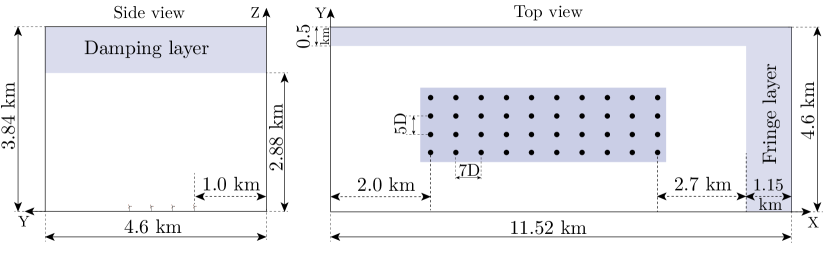
Figure 3: Schematic to show the wind farm layout with the damping layer to prevent gravity waves and the fringe layer used in the concurrent precursor method. The black circles denote the wind turbine locations. All the flow statistics are sampled from the shaded region with dimensions $70D\times{20D}\times{D}$ centered around the wind farm; see also figure 6.

The computational domain is $11.52$ km $\times$ $4.6$ km $\times$ $3.84$ km, which is discretized by $1280\times 512\times 384$ grid points. The grid points are uniformly distributed in horizontal directions. This leads to a uniform grid resolution of 9 m in both streamwise and spanwise directions. In the vertical direction a grid spacing of 5 m is used up to 1500 m, above which the grid is slowly stretched. Here we emphasize that our simulations benefit from using an advanced Lagrangian dynamic SGS scale model, which has been shown to capture the dynamics of stable boundary layers very well Stoll and Porté-Agel (2008); Gadde and Stevens (2019). It is worth mentioning here that in the LES intercomparison of the most widely studied stable boundary layer, Beare et al. Beare et al. (2006) report that a grid size of 6.25 m produces reasonably acceptable results compared to high-resolution LES of stable boundary layers. To provide perspective, recently, Allaerts and Meyers Allaerts and Meyers (2018) in the simulation of wind farms in a stable boundary layer, used a horizontal resolution of 12.5 m and a vertical resolution of 5 m. Furthermore, Ali et al. Ali et al. (2017) in their simulations of wind farms in diurnal cycles, which also includes stable boundary layers, use a horizontal resolution of 24.5 m and a vertical resolution of 7.8 m. So the resolution employed here is relatively high for simulations of such large wind farms.
We employ the concurrent precursor technique Stevens, Graham, and Meneveau (2014) to introduce the inflow conditions sampled from the precursor simulation into the wind farm domain. LLJs generally occur over small regions and have limited spanwise width. Therefore, we use fringe layers in both streamwise and spanwise directions to remove the effect of periodicity. A Rayleigh damping layerKlemp and Lilly (1978) with a damping constant of 0.016 $\text{s}^{-1}$ is used in the top 25$\%$ of the domain to damp out the gravity waves triggered by the wind farm.
We consider a wind farm with 40 turbines distributed in 4 columns and 10 rows, see Fig. 2. We choose turbines of diameter, $D=80$ m and the turbines are separated by a distance of $7D$ and $5D$ in the streamwise and spanwise directions, respectively. The objective of our study is to study the effect of $z_{\text{jet}}/z_{h}$ on wake recovery and wind farm power production. To achieve that, we vary the turbine hub height such that $z_{\text{jet}}>z_{h}$, $z_{\text{jet}}{\approx}z_{h}$, and $z_{\text{jet}}<z_{h}$, corresponding hub-heights are $z_{h}=0.5z_{\text{jet}}$, $z_{\text{jet}}$, $1.5z_{\text{jet}}$. The three cases represent the scenarios when the LLJ is below, above, and in the middle of the turbine rotor swept area. We perform two additional simulations with $z_{h}/D=0.75$ and turbine diameters 160 m and 240 m to study the effect of turbine diameter on wind farm performance. In these simulations, the turbines are separated by $720$ m in the streamwise direction. In the spanwise direction, for the cases with turbine diameter $160$ m and $240$ m, the turbines are separated by $480$ m and $720$ m, respectively.
Calaf et al. Calaf, Meneveau, and Meyers (2010) and Meyers and Meneveau Meyers and Meneveau (2013) showed that a resolution of $25$ m $\leq\Delta{x}\leq$ $50$ m in the streamwise direction and of $10$ m $\leq\Delta{y}\leq$ $25$ m in the spanwise direction is sufficient when an actuator disk method is used to model the turbines. Furthermore, Wu and Porté-Agel Wu and Porté-Agel (2011) showed that one needs $8$ points along the diameter in the vertical direction and $5$ points along the diameter in the spanwise direction. Clearly, our simulations satisfy these criteria as we use a $5$ m resolution in the vertical and a $9$ m resolution in the horizontal directions. This means the turbine disk is discretized by $16$ points in the vertical and  $9$ points in the spanwise direction, respectively.
We use a proportional-integral (PI) controllerAllaerts and Meyers (2015) to ensure that the mean wind direction at hub-height is from West to East. The wind angle controller has been successfully used in our previous study of wind farms in neutral and stable boundary layers Gadde and Stevens (2019) and ensures that the wind farm geometry is the same for all considered cases. Yaw misalignment due to the local changes in the wind angle is prevented by rotating the actuator disks such that the disks are always perpendicular to the local wind angle. Figure 3 shows the wind farm layout and the dimensions of the different regions in the computational domain.

III Results & discussions

The simulations were carried out in two stages. In the first stage, only the boundary layer in the precursor domain is simulated. After the quasi-steady conditions are reached, the turbines are introduced at the end of the 8${}^{\text{th}}$ hour. In this second stage, the simulations are continued for two more hours, and the statistics are collected in the last hour. Each simulation costs about 0.3 million CPU hours. In section III.1 the flow structures are analyzed, followed by a discussion on power production, momentum flux, and wake recovery in section III.2. In section III.3, an energy budget analysis is presented in which we discuss the diverse processes affecting the wind farm performance in the presence of a LLJ.

III.1 Flow structures

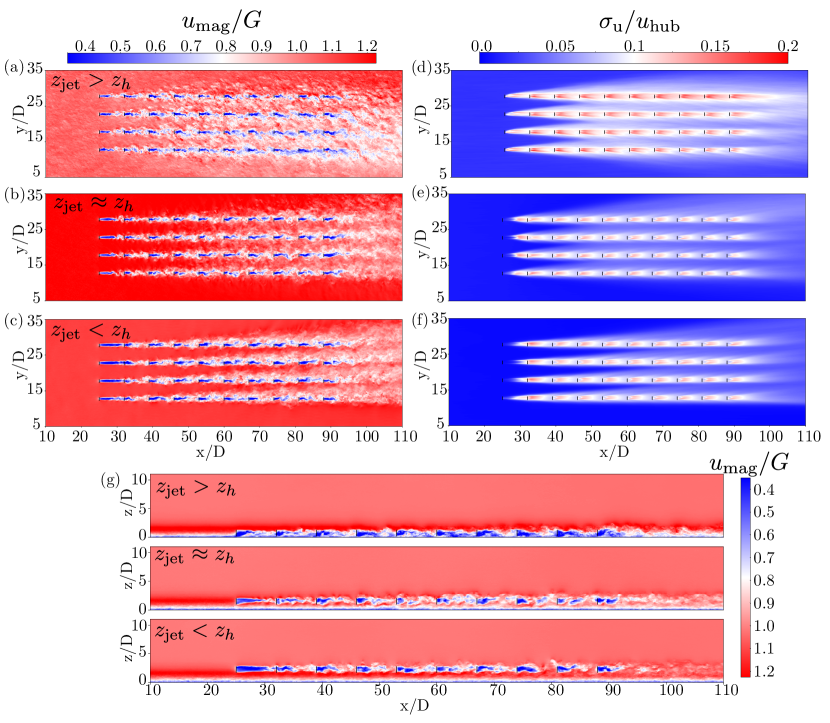
Figure 4: Normalized instantaneous velocity $u_{\text{mag}}/G$ at hub-height for the three cases, i.e. (a) $z_{\text{jet}}>z_{h}$, (b) $z_{\text{jet}}\approx z_{h}$, and (c) $z_{\text{jet}}<z_{h}$. Figs. (d), (e), and (f) present the corresponding time-averaged turbulence intensity, $\sigma_{u}/u_{\text{hub}}$ where $\sigma_{u}=\sqrt{2k/3}$ and k is the turbulent kinetic energy. (g) Side view of the instantaneous streamwise velocity in an x-z plane through the second turbine column for the different cases.

A visualization of the instantaneous velocity at hub-height is presented in Figs. 4(a), (b), and (c). Figures 4(d), (e), and (f) show the time-averaged turbulence intensity for all three cases. The turbulence intensity is calculated as $\sigma_{u}=\sqrt{2k/3}$, where $k=0.5(\overline{u^{\prime 2}}+\overline{v^{\prime 2}}+\overline{w^{\prime 2}})$ is the resolved turbulent kinetic energy and $u_{\text{hub}}=\sqrt{\overline{{u}}^{2}+\overline{{v}}^{2}+\overline{{w}}^{2}}$ is the velocity at the hub-height at the inlet. When the LLJ is above the turbines, small scale structures are visible in the entrance region in front of the wind farm, see Fig. 4(a). In this case, the turbines operate in a completely turbulent region, and the wakes show significant turbulence towards the end of the wind farm, see Fig. 4(d). The wakes recover relatively fast due to the high atmospheric turbulence and the additional wake generated turbulence. In contrast, Figs. 4(b) and 4(e) show less turbulence in the entrance region of the wind farm and behind the first turbine row for the $z_{h}\approx z_{\text{jet}}$ case. However, towards the rear of the wind farm, we observe significant turbulence. This effect is prominent when the LLJ is below the turbines ($z_{\text{jet}}<z_{h}$), and we observe only marginal wake turbulence behind the first turbine row, see Fig. 4(c) and 4(f). This will affect the wake recovery and consequently the power production of the second turbine row. The limited turbulence at hub-height at the farm entrance is due to the strong thermal stratification associated with the surface inversion top. However, after the first couple of rows, we observe significant turbulence created by the wakes. It is widely accepted that the turbine wake meandering and corresponding wake turbulence is related to the atmospheric turbulence Mao and Sørensen (2018); Larsen et al. (2008), and in the absence of atmospheric turbulence, the wake turbulence is also limited. In essence, the wake recovery is affected when turbines operate in the negative shear region above the LLJ.

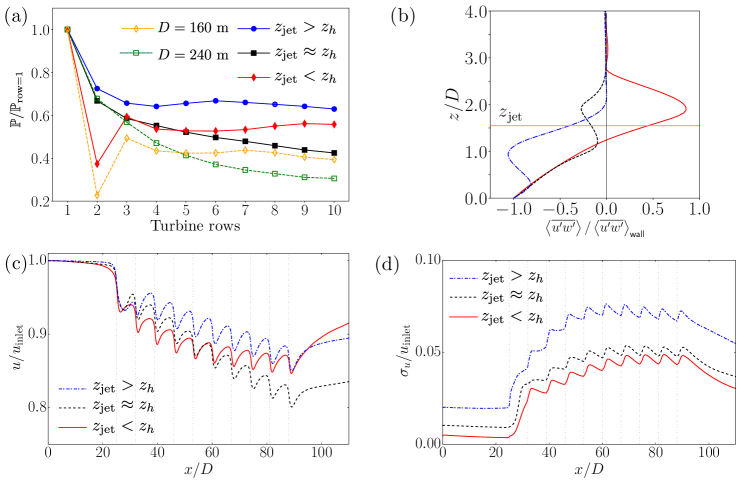
Figure 5: (a) The row-averaged power normalized with the power production of the first row. Results from the additional simulations with $D=160$ m and $D=240$ m are also included. (b) Planar averaged streamwise vertical momentum flux versus height. (c) Spanwise averaged streamwise velocity normalized with the upstream velocity at hub-height as a function of the streamwise location. (d) Streamwise variation of the turbulence intensity at hub-height for the three different cases.

Figure 4(g) shows the side view of the wind farm in an x-z plane passing through the second turbine column. The top panel in Fig. 4(g) shows the turbines operating in a turbulent region. It is worth noting that the turbine wakes show significant wake turbulence, which aids the extraction of momentum from the LLJ. When $z_{\text{jet}}\approx z_{h}$, the turbines in the first row extract the energy in the jet, and turbines operate in a well-mixed region after the second turbine row. Moreover, the LLJ reduces in strength after the first turbine row, and therefore rows that are further downstream cannot benefit from the jet anymore. However, when the LLJ is below the turbines ($z_{\text{jet}}<z_{h}$), the first couple of turbine rows are in a non-turbulent region, and therefore the turbulence after the first turbine row is limited. Furthermore, we observe no transverse wake meandering behind the first turbine row due to low atmospheric turbulence in the thermally stratified region above the jet. The jet’s strength is reduced due to energy extraction towards the rear of the wind farm because of the positive entrainment flux created from below due to the energy extraction by turbines. This will be discussed in detail in the next section.

III.2 Power production and wake recovery

The row-averaged power normalized by the first row’s power production is presented in Fig. 5(a). The turbine power is averaged in the $10^{\text{th}}$ hour of the simulation. Results from the additional simulations with the diameters $160$ m and $240$ m are also included in the figure. When the LLJ is above the turbines ($z_{\text{jet}}>z_{h}$), we observe that the relative power production is higher, which means that velocity recovers faster than in the other cases, see the plot of wake recovery in Fig. 5(c). When $z_{h}\approx z_{\text{jet}}$, the power production continuously reduces towards the rear of the wind farm, see Fig. 5(a). The corresponding wake recovery shows that the velocity continuously drops in the downstream direction, which indicates that the wake recovery is negligible; see the dashed line in Fig. 5(c). Interestingly, when the jet is below the turbines ($z_{\text{jet}}<z_{h}$), the power production of the second row is severely affected due to the absence of turbulence in the wake of the first turbine row. However, the power production increases further downstream due to wake generated turbulence, and it shows an upward trend towards the back of the wind farm. For this case, the wake turbulence becomes significant for $x/D>30$ behind the second turbine row, and subsequently, the turbines entrain high momentum wind from the LLJ, and the wake recovers significantly. For the additional cases with turbines with bigger diameter of 160 m and 240 m, we find that the overall trends in the normalized power production as a function of the downstream position remains the same even though the streamwise turbine spacing is small. This confirms that the results presented in this study capture the relevant physics of the different scenarios, i.e. when the LLJ is below, in the middle, or above the turbine rotor swept area.
To understand the wake recovery and the associated power production of downstream turbines, the planar averaged vertical turbulent flux of streamwise momentum $\left<\overline{u^{\prime}w^{\prime}}\right>$ and normalized by the $\left<\overline{u^{\prime}w^{\prime}}\right>$ at the wall are plotted in Fig. 5(b). When the LLJ is above the turbine rotor swept area ($z_{\text{jet}}>z_{h}$), there is a significant negative (downward) momentum flux, which extracts the jet’s momentum and eliminates it towards the rear of the wind farm. However, when the LLJ is below the turbines ($z_{\text{jet}}<z_{h}$), the turbines operate in the negative shear region, and a significant positive entrainment flux is created. As a result, the jet’s energy is entrained towards the turbines, and the power production shows an upward trend towards the end of the wind farm, see Fig. 5(a). In essence, when the LLJ is below the turbine rotor swept area, the momentum deficit by the turbines creates a significant positive turbulent flux from below due to the negative shear. This enhances the wake recovery further downstream which is further elucidated below.
For continuous production of turbulence $\overline{u^{\prime}w^{\prime}}\frac{\partial{\overline{u}}}{\partial{z}}$ should be negative. Therefore, in the presence of positive shear ($\frac{\partial{\overline{u}}}{\partial{z}}$ is positive) $\overline{u^{\prime}w^{\prime}}$ should be negative to produce turbulence. However, when the shear is negative ($\frac{\partial{\overline{u}}}{\partial{z}}$ is negative) $\overline{u^{\prime}w^{\prime}}$ should be positive to sustain turbulence. The tendency of the velocity deficit in the turbine wakes is to create a positive entrainment flux below the hub-height and a negative entrainment flux above hub-height. This leads to the following two scenarios:

• When the LLJ is above the turbine rotor swept area ($z_{\text{jet}}>z_{h}$), LLJ energy is pulled towards the turbines due to the momentum deficit created by the turbines. We have a significant downward entrainment flux, which is utilized by the turbines for power production. Due to which the LLJ strength is reduced. In this case, $\overline{u^{\prime}w^{\prime}}$ is negative, and the horizontally averaged $\frac{\partial{\overline{u}}}{\partial{z}}$ is positive, and there is a net negative vertical flux towards the turbines.

• When the LLJ is below the turbine rotor swept area ($z_{\text{jet}}<z_{h}$), the high momentum LLJ with the positive entrainment flux from below aid power production. The turbines extract the LLJ energy transported by the positive entrainment fluxes. In this case, $\overline{u^{\prime}w^{\prime}}$ is positive and the horizontally averaged $\frac{\partial{\overline{u}}}{\partial{z}}$ is negative. The negative shear created by the wind turbine wakes contributes to the negative shear already present above the LLJ, and this aids power production of downstream turbines.

To quantify the turbulence produced by the wakes, the streamwise variation of the horizontally averaged turbulence intensity at the hub-height is plotted in Fig. 5(d). When the LLJ is above the turbine rotor ($z_{\text{jet}}>z_{h}$), the turbulence intensity upstream of the farm is 1.97%, while it is 1.0% and 0.46% for $z_{\text{jet}}\approx z_{h}$ and $z_{\text{jet}}<z_{h}$, respectively. We observe negligible wake turbulence behind the first turbine row in Fig. 4(d) when the LLJ is below the turbine rotor swept area ($z_{h}>{z_{\text{jet}}}$). However, after turbulence is created by the wakes, the turbulence intensity increases to about approximately $4.4\%$ further downstream. It is clear from the above data that there is limited upstream turbulence when the LLJ is below the turbine rotor swept area. Consequently, there is negligible wake recovery until there is a wake generated turbulence. In essence, the negative shear above the jet creates a positive entrainment flux, which increases the turbulence intensity when the LLJ is below the turbine rotor swept area. This accelerates the wake recovery and allows the turbines to extract energy from the jet. The turbulence intensity for the $z_{\text{jet}}\approx z_{h}$ case develops in a very similar way as for the ${z_{\text{jet}}}<z_{h}$ case as in both cases it is mostly determined by the wake added turbulence. However, when the LLJ is above the turbine rotor swept area, the turbulence intensity inside the wind farm is higher as the atmospheric turbulence interacts with the wind turbine wakes.

III.3 Energy budget analysis

To further understand the different processes involved in the power production of a wind farm in the presence of a LLJ we perform an energy budget analysis. The analysis is similar to the budget analysis performed by Allaerts and Meyers (Allaerts and Meyers, 2017) for wind farms in conventionally neutral boundary layers. The steady-state, time-averaged energy equation is obtained by multiplying equation (2) with $\widetilde{u}_{i}$Allaerts and Meyers (2017); Sagaut (2006) and performing time-averaging, which results in:

$$\centering\begin{split}&\overbrace{\overline{u}_{j}\partial_{j}\left({\frac{1}{2}\overline{u}_{i}\overline{u}_{i}}+\frac{1}{2}\overline{u^{\prime}_{i}u^{\prime}_{i}}\right)}^{\text{Kinetic energy flux}}+\overbrace{\partial_{j}\left(\frac{1}{2}{\overline{u^{\prime}_{j}u^{\prime}_{i}u^{\prime}_{i}}}+\overline{u}_{i}\overline{u^{\prime}_{i}u^{\prime}_{j}}\right)}^{\text{ Turbulent transport}}+\overbrace{\partial_{j}\left(\overline{u_{i}\tau_{ij}}\right)}^{\text{SGS transport}}\\ &=\overbrace{-\partial_{i}{\left(\overline{pu_{i}}\right)}}^{\text{Flow work}}+\overbrace{g\beta(\overline{u_{i}\theta}-\overline{u}_{i}\theta_{0})\delta_{i3}}^{\text{Buoyancy}}+\overbrace{f_{c}\left(\overline{u}_{i}U_{g}\right)\delta_{i2}-f_{c}\left(\overline{u}_{i}V_{g}\right)\delta_{i1}}^{\text{Geostrophic forcing}}\\ &+\overbrace{\overline{f_{i}u_{i}}}^{\text{Turbine power}}+\overbrace{\overline{\tau_{ij}S_{ij}}}^{\text{Dissipation}},\end{split}\@add@centering$$ (10)

where the time-averaging is represented by the overline, and $\overline{u^{\prime}_{i}u^{\prime}_{j}}=\left(\overline{{u_{i}u_{j}}}\right)-\overline{{u}_{i}}~{}\overline{{u}_{j}}$ indicates the momentum fluxes. To obtain the total power produced by each row we numerically integrate each term in equation (10) around a control volume surrounding each row. The control volume is chosen such that it encloses a row of wind farm, see Fig. 6. We note here that the fringe layers are not included in the control volume. Performing integration and rearranging equation (10) gives,

$$\centering\begin{split}\overbrace{\int_{\forall}\overline{f_{i}u_{i}}d\forall}^{\text{$\mathbb{P}$, Turbine power}}&=\overbrace{\int_{\forall}\overline{u}_{j}\partial_{j}\left({\frac{1}{2}\overline{u}_{i}\overline{u}_{i}}+\frac{1}{2}\overline{u^{\prime}_{i}u^{\prime}_{i}}\right)d\forall}^{\text{$\mathbb{E}_{k}$, Kinetic energy flux}}\\ &+\overbrace{\int_{\forall}\partial_{j}\left(\frac{1}{2}{\overline{u^{\prime}_{j}u^{\prime}_{i}u^{\prime}_{i}}}+\overline{u}_{i}\overline{u^{\prime}_{i}u^{\prime}_{j}}\right)d\forall}^{\text{$\mathbb{T}_{\text{t}}$, Turbulent transport}}+\overbrace{\int_{\forall}\partial_{j}\left(\overline{u_{i}\tau_{ij}}\right)d\forall}^{\text{$\mathbb{T_{\text{sgs}}}$, SGS transport}}\\ &+\overbrace{\int_{\forall}\partial_{i}{\left(\overline{pu_{i}}\right)}d\forall}^{\text{$\mathbb{F}$, Flow work}}-\overbrace{\int_{\forall}g\beta(\overline{u_{i}\theta}-\overline{u}_{i}\theta_{0})\delta_{i3}d\forall}^{\text{$\mathbb{B}$, Buoyancy}}\\ &-\overbrace{\int_{\forall}f_{c}\left(\overline{u}_{i}U_{g}\right)\delta_{i2}-f_{c}\left(\overline{u}_{i}V_{g}\right)\delta_{i1}d\forall}^{\text{$\mathbb{G}$, Geostrophic forcing}}-\overbrace{\int_{\forall}\overline{\tau_{ij}S_{ij}}d\forall,}^{\text{$\mathbb{D}$, Dissipation}}\end{split}\@add@centering$$ (11)

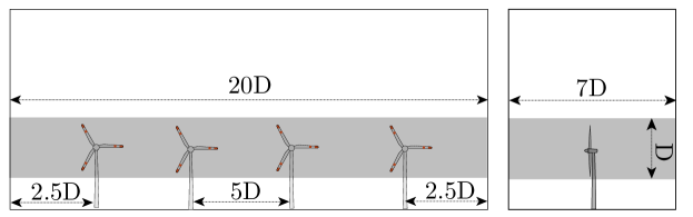
Figure 6: The shaded region shows the control volume used in the energy budget analysis. The control volume around each turbine row has dimensions of $7\text{D}\times{20\text{D}}\times{\text{D}}$ in the streamwise, spanwise, and vertical directions, respectively. In the vertical direction the control volume starts at a height of $z_{h}-D/2$.

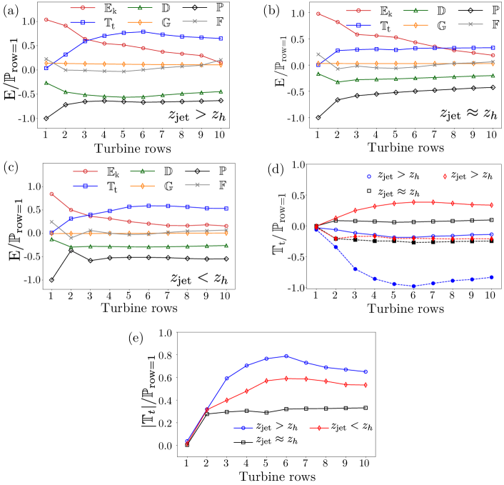
Figure 7: Energy budget for (a) $z_{\text{jet}}>z_{h}$ (b) $z_{\text{jet}}\approx z_{h}$ and (c) $z_{\text{jet}}<z_{h}$. (d) Integrated entrainment flux over top and bottom planes of the control volume. Dashed lines with filled symbols and solid lines with open symbols represent $\mathbb{T}_{t}$ on the top and bottom plane, respectively. (e) Normalized net entrainment for different cases.

where $\mathbb{P}$ is the power produced by a turbine row, $\mathbb{E}_{k}$ is the kinetic energy flux containing resolved kinetic energy, $\mathbb{T}_{t}$ is the turbulent transport, which involves the transport of mean flow energy by turbulence Tennekes and Lumley (1972) and higher-order turbulence terms, $\mathbb{T}_{\text{sgs}}$ is the mean energy transport by SGS stresses, $\mathbb{F}$ is the flow work, which is the pressure drop across the turbines, $\mathbb{B}$ is the turbulence destruction caused by buoyancy under stable stratification, $\mathbb{G}$ represents the geostrophic forcing driving the flow, and $\mathbb{D}$ is the SGS dissipation.
Figure 7(a), (b), and (c) present the energy budget analysis for cases when the LLJ is above ($z_{\text{jet}}>z_{h}$), in the middle ($z_{\text{jet}}\approx z_{h}$), or below ($z_{\text{jet}}<z_{h}$) the turbine rotor swept area, respectively. All the terms are normalized by the absolute value of the power produced by the first turbine row. This normalization provides insight into the effect of wake recovery on power production. The SGS transport term $\mathbb{T}_{\text{sgs}}$ and the buoyancy terms $\mathbb{B}$ are negligible and left out of the plots for brevity. In both plots, the energy sources are positive, and sinks are negative. Both turbine power and dissipation act as energy sinks in the boundary layer. Fig. 7(a) shows that when the LLJ is above the turbine rotor swept area ($z_{\text{jet}}>z_{h}$), the kinetic energy $\mathbb{E}_{k}$ continuously decreases in the downstream direction. This reduction in the mean kinetic energy is compensated by the turbulent transport term $\mathbb{T}_{t}$. The turbulent transport slightly reduces after the sixth turbine row due to the reduction in the strength of the LLJ. In this case, the downward entrainment of the fluxes compensates for the decrease in mean kinetic energy. In a fully developed wind farm boundary layer, the power production is completely balanced by the turbulent entrainment from above Calaf, Meneveau, and Meyers (2010); Cal et al. (2010). When the turbines operate in the positive shear region, the entrainment from above replenishes the energy extracted by the turbines. In addition to entrainment, the geostrophic forcing $\mathbb{G}$ and pressure drop $\mathbb{F}$ act as an additional energy source. In contrast, turbulence destruction by buoyancy $\mathbb{B}$ and dissipation $\mathbb{D}$ remove energy from the control volume. When the LLJ is above the turbine rotor swept area ($z_{\text{jet}}>z_{h}$), there is positive shear in the boundary layer, due to which there is significant entrainment and wake recovery.
When the LLJ is in the middle of the turbine rotor swept area ($z_{\text{jet}}\approx z_{h}$), while the kinetic energy $\mathbb{E}_{k}$ continuously decreases the entrainment $\mathbb{T}_{t}$ is reduced as the energy in the LLJ is extracted by the upwind turbines reducing the entrainment for the rest of the turbines. Furthermore, turbulent entrainment $\mathbb{T}_{t}$ is nearly equal to the turbulence dissipation $\mathbb{D}$, this limits the contribution of turbulence to power production. When the LLJ is below the turbine rotor swept area ($z_{\text{jet}}<z_{h}$), the kinetic energy $\mathbb{E}_{k}$ contribution decreases continuously with downstream position in the wind farm and the turbulent transport $\mathbb{T}_{t}$ is less than for the case when the LLJ is above the turbines (Fig. 7(c)). The turbulent transport $\mathbb{T}_{t}$ is created entirely by the wake turbulence and the momentum deficit created by the turbines. The power production is mainly due to the mean flow energy extraction $\mathbb{E}_{k}$ and the entrainment due to positive entrainment flux. In essence, the wake recovery and the entrainment due to turbulent transport are affected when the LLJ is below the turbine rotor swept area.
To further elucidate the effect of entrainment on power production, we plot the integrated vertical entrainment flux on the top and bottom planes of the control volume in Fig. 7(d). Open symbols represent the integrated flux on the bottom plane, and filled symbols represent the integrated flux on the top plane of the control volume. When the LLJ is above the turbine rotor swept area ($z_{\text{jet}}>z_{h}$), the negative flux from the top is dominant. However, when the LLJ is below the turbine rotor swept area ($z_{\text{jet}}<z_{h}$), there is significant positive flux in the bottom plane indicating positive entrainment from below. This clearly shows that there is significant positive entrainment flux towards the turbine rotors when the LLJ is below the turbine rotor swept area. This is beneficial for the power production of turbines further downstream.
Figure 7(e) provides a comparison of the net entrainment $|\mathbb{T}_{t}|$ for all the three cases. The figure shows that entrainment is strongest when the LLJ is above the turbine rotor swept area ($z_{\text{jet}}>z_{h}$) and least when $z_{\text{jet}}\approx z_{h}$. When the LLJ is in the middle of the turbine rotor swept area ($z_{\text{jet}}\approx z_{h}$) the entrainment is affected as the LLJ energy is mostly extracted by the turbines in the first couple of rows. When the LLJ is below the turbine rotor swept area ($z_{\text{jet}}<z_{h}$), there is increased entrainment due to the positive entrainment flux. This creates a stronger turbulent transport $\mathbb{T}_{t}$ than for the $z_{\text{jet}}\approx z_{h}$ case, but not as much as for the case when the LLJ is above the turbine rotor swept area.

IV Conclusions

We performed LES of wind farms to study the effect of the LLJ height compared to the turbine-height on the interaction between LLJs and large wind farms, see Fig. 1. We considered three scenarios, wherein the LLJ is above, below, and in the middle of the turbine rotor swept area. We find that the relative power production of the turbines further downstream in the wind farm depends on the jet height relative to the hub-height. The power production relative to the first-row power is maximum when the LLJ is above the turbine rotor swept area due to higher turbulence intensity below the LLJ, wherein the atmospheric turbulence adds to the turbine wake generated turbulence and leads to a faster wake recovery. However, when the LLJ is below the turbine rotor swept area, the turbines operate in the negative shear region of the LLJ in which the atmospheric turbulence is limited, and the thermal stability is strong. In the absence of atmospheric turbulence, the wakes are very stable Mao and Sørensen (2018); Keck et al. (2014), and wake recovery is slow. However, after the first two turbine rows, the wakes generate sufficient turbulence to promote the wake recovery further downstream.
The energy budget analysis reveals that the vertical entrainment dominates the power production when the LLJs are above the turbine rotor swept area. In contrast, when the LLJ is in the middle of the turbine rotor swept area, the jet’s energy is extracted by the first turbine row, and the rest of the rows do not directly benefit from the jet. Interestingly, when the LLJ is below the turbine rotor swept area, the mean negative shear and the shear created by the wakes create a positive entrainment flux from below, which helps turbines further downstream to harvest the jet’s energy. Although the negative shear above the LLJ creates a positive turbulent entrainment flux, the turbulence production it creates is limited due to the high thermal stratification above the jet, i.e. the flux that is created is smaller than the flux that is created when the LLJ is above the turbines.
Gutierrez et al. Gutierrez et al. (2017) report the reduction in the turbine loads due to the negative shear in the LLJ and therefore suggest installing turbines such that they are in this region. Our results show that wake recovery is affected when the turbines operate in the negative shear region, and therefore, it might not be beneficial in terms of wake recovery. Here, we emphasize again that we used a generalized LLJ to study the physical phenomena that result from the interaction of a LLJ with a large wind farm. However, further work will be required to investigate the effect of higher thermal stratification, complex terrain, the strength of the geostrophic wind and its direction, the transition from land to sea on the LLJ characteristics, and how this affects the performance of wind farms.

author’s contributions

All authors contributed equally to the manuscript.

Data availability

The data that support the findings of this study are available from the corresponding author upon reasonable request.

References

References

- Abkar, Sharifi, and Porté-Agel (2016) Abkar, M., Sharifi, A., and Porté-Agel, F., “Wake flow in a wind farm during a diurnal cycle,” J. Turb. 625, 012031 (2016).
- Ali et al. (2017) Ali, N., Cortina, G., Hamilton, N., Calaf, M., and Cal, R. B., “Turbulence characteristics of a thermally stratified wind turbine array boundary layer via proper orthogonal decomposition,” J. Fluid Mech. 828, 175–95 (2017).
- Ali et al. (2018) Ali, N., Hamilton, N., Cortina, G., and Calaf, M., “Anisotropy stress invariants of thermally stratified wind turbine array boundary layers using large eddy simulations,” J. Renew. Sustain. Energy 10, 013301 (2018).
- Allaerts and Meyers (2015) Allaerts, D. and Meyers, J., “Large eddy simulation of a large wind-turbine array in a conventionally neutral atmospheric boundary layer,” Phys. Fluids 27, 065108 (2015).
- Allaerts and Meyers (2017) Allaerts, D. and Meyers, J., “Boundary-layer development and gravity waves in conventionally neutral wind farms,” J. Fluid Mech. 814, 95–130 (2017).
- Allaerts and Meyers (2018) Allaerts, D. and Meyers, J., “Gravity waves and wind-farm efficiency in neutral and stable conditions,” Boundary-Layer Meteorol. 166, 269 (2018).
- Arritt et al. (1997) Arritt, R. W., Rink, T. D., Segal, M., Todey, D. P., Clark, C. A., Mitchell, M. J., and Labas, K. M., “The Great Plains low-level jet during the warm season of 1993,” Mon. Weather Rev. 125, 2176–2192 (1997).
- Baas et al. (2009) Baas, P., Bosveld, F. C., Baltink, H. K., and Holtslag, A. A. M., “A climatology of nocturnal low-level jets at Cabauw,” J. Appl. Meteor. Climatol. 48, 1627–1642 (2009).
- Banta (2008) Banta, R. M., “Stable-boundary-layer regimes from the perspective of the low-level jet,” Acta Geophysica 56, 58–87 (2008).
- Banta et al. (2002) Banta, R. M., Newsom, R. K., Lundquist, J. K., Pichugina, Y. L., Coulter, R. L., and Mahrt, L., “Nocturnal low-level jet characteristics over Kansas during CASES-99,” Boundary-Layer Meteorol. 105, 221–252 (2002).
- Beare et al. (2006) Beare, R. J., Macvean, M. K., Holtslag, A. A. M., Cuxart, J., Esau, I., Golaz, J.-C., Jimenez, M. A., Khairoutdinov, M., Kosovic, B., Lewellen, D., Lund, T. S., Lundquist, J. K., Mccabe, A., Moene, A. F., Noh, Y., Raasch, S., and Sullivan, P., “An intercomparison of large eddy simulations of the stable boundary layer,” Boundary-Layer Meteorol. 118, 247–272 (2006).
- Bhaganagar and Debnath (2015) Bhaganagar, K. and Debnath, M., “The effects of mean atmospheric forcings of the stable atmospheric boundary layer on wind turbine wake,” J. Renew. Sustain. Energy 7, 013124 (2015).
- Blackadar (1957) Blackadar, A. K., “Boundary layer wind maxima and their significance for the growth of nocturnal inversions,” Bull. Am. Meteorol. Soc. 38, 283–290 (1957).
- Bou-Zeid, Meneveau, and Parlange (2005) Bou-Zeid, E., Meneveau, C., and Parlange, M. B., “A scale-dependent Lagrangian dynamic model for large eddy simulation of complex turbulent flows,” Phys. Fluids 17, 025105 (2005).
- Brutsaert (1982) Brutsaert, W., Evaporation into the atmosphere: theory, history and applications, Vol. 1 (1982).
- Cal et al. (2010) Cal, R. B., Lebrón, J., Castillo, L., Kang, H. S., and Meneveau, C., “Experimental study of the horizontally averaged flow structure in a model wind-turbine array boundary layer,” J. Renew. Sustain. Energy 2, 013106 (2010).
- Calaf, Meneveau, and Meyers (2010) Calaf, M., Meneveau, C., and Meyers, J., “Large eddy simulations of fully developed wind-turbine array boundary layers,” Phys. Fluids 22, 015110 (2010).
- Calaf, Parlange, and Meneveau (2011) Calaf, M., Parlange, M. B., and Meneveau, C., “Large eddy simulation study of scalar transport in fully developed wind-turbine array boundary layers,” Phys. Fluids 23, 126603 (2011).
- Canuto et al. (1988) Canuto, C., Hussaini, M. Y., Quarteroni, A., and Zang, T. A., Spectral Methods in Fluid Dynamics (Springer, Berlin, 1988).
- Doosttalab et al. (2020) Doosttalab, A., Siguenza-Alvarado, D., Pulletikurthi, V., Jin, Y., Evans, H. B., Chamorro, L. P., and Castillo, L., “Interaction of low-level jets with wind turbines: On the basic mechanisms for enhanced performance,” J. Renew. Sustain. Energy 12, 053301 (2020).
- Dörenkämper et al. (2015) Dörenkämper, M., Witha, B., Steinfeld, G., Heinemann, D., and Kühn, M., “The impact of stable atmospheric boundary layers on wind-turbine wakes within offshore wind farms,” J. Wind Eng. Ind. Aerodyn. 144, 146–153 (2015).
- Duncan (2018) Duncan, J. B., Observational analyses of the North Sea low-level jet (Petten: TNO, 2018).
- Ferziger and Perić (2002) Ferziger, J. H. and Perić, M., Computational methods for fluid dynamics (Springer, 2002).
- Fitch, Olson, and Lundquist (2013) Fitch, A. C., Olson, J. B., and Lundquist, J. K., “Parameterization of wind farms in climate models,” J. Wind Eng. Ind. Aerodyn. 26, 6439–6458 (2013).
- Gadde and Stevens (2019) Gadde, S. N. and Stevens, R. J. A. M., “Effect of Coriolis force on a wind farm wake,” J. Phys. Conf. Ser. 1256, 012026 (2019).
- Gadde and Stevens (2020) Gadde, S. N. and Stevens, R. J. A. M., “Interaction between low-level jets and wind farms in a stable atmospheric boundary layer,” submitted (2020).
- Gadde, Stieren, and Stevens (2020) Gadde, S. N., Stieren, A., and Stevens, R. J. A. M., “Large-eddy simulations of stratified atmospheric boundary layers: Comparison of different subgrid models,” Boundary-Layer Meteorol. , 1–20 (2020).
- Greene et al. (2009) Greene, S., McNabb, K., Zwilling, R., Morrissey, M., and Stadler, S., “Analysis of vertical wind shear in the southern great plains and potential impacts on estimation of wind energy production,” Int. J. Global Energy 32, 191–211 (2009).
- Gutierrez et al. (2016) Gutierrez, W., Araya, G., Kiliyanpilakkil, P., Ruiz-Columbie, A., Tutkun, M., and Castillo, L., “Structural impact assessment of low level jets over wind turbines,” J. Renew. Sustain. Ener. 8, 023308 (2016).
- Gutierrez et al. (2017) Gutierrez, W., Ruiz-Columbie, A., Tutkun, M., and Castillo, L., “Impacts of the low-level jet’s negative wind shear on the wind turbine,” Wind Energy Science 2, 533–545 (2017).
- Holtslag and Nieuwstadt (1986) Holtslag, A. A. M. and Nieuwstadt, F. T. M., “Scaling the atmospheric boundary layer,” Boundary-Layer Meteorol. 36, 201–209 (1986).
- Jimenez et al. (2007) Jimenez, A., Crespo, A., Migoya, E., and Garcia, J., “Advances in large-eddy simulation of a wind turbine wake,” J. Phys. Conf. Ser. 75, 012041 (2007).
- Jimenez et al. (2008) Jimenez, A., Crespo, A., Migoya, E., and Garcia, J., “Large-eddy simulation of spectral coherence in a wind turbine wake,” Environ. Res. Lett. 3, 015004 (2008).
- Kalverla et al. (2019) Kalverla, P. C., Duncan Jr., J. B., Steeneveld, G.-J., and Holtslag, A. A. M., “Low-level jets over the North Sea based on ERA5 and observations: together they do better,” Wind Energy Science 4, 193–209 (2019).
- Kalverla et al. (2017) Kalverla, P. C., Steeneveld, G.-J., Ronda, R. J., and Holtslag, A. A. M., “An observational climatology of anomalous wind events at offshore meteomast IJmuiden (North Sea),” J. Wind. Eng. Ind. Aerodyn. 165, 86–99 (2017).
- Keck et al. (2014) Keck, R. E., de Maré, M., Churchfield, M. J., Lee, S., Larsen, G., and Madsen, H. A., “On atmospheric stability in the dynamic wake meandering model,” Wind Energy 17, 1689–1710 (2014).
- Kelley et al. (2004) Kelley, N., Shirazi, M., Jager, D., Wilde, S., Adams, J., Buhl, M., Sullivan, P., and Patton, E., “Lamar low-level jet project interim report,” National Renewable Energy Laboratory, National Wind Technology Center, Golden, CO, Technical Paper No. NREL/TP-500-34593 (2004).
- Klemp and Lilly (1978) Klemp, J. B. and Lilly, D. K., “Numerical simulation of hydrostatic mountain waves,” J. Atmos. Sci. 68, 46–50 (1978).
- van Kuik et al. (2016) van Kuik, G. A. M., Peinke, J., Nijssen, R., Lekou, D., Mann, J., Sørensen, J. N., Ferreira, C., van Wingerden, J. W., Schlipf, D., Gebraad, P., Polinder, H., Abrahamsen, A., van Bussel, G. J. W., Srensen, J. D., Tavner, P., Bottasso, C. L., Muskulus, M., Matha, D., Lindeboom, H. J., Degraer, S., Kramer, O., Lehnhoff, S., Sonnenschein, M., Srensen, P. E., Künneke, R. W., Morthorst, P. E., and Skytte, K., “Long-term research challenges in wind energy - a research agenda by the European Academy of Wind Energy,” Wind Energy Science 1, 1–39 (2016).
- Kumar et al. (2010) Kumar, V., Svensson, G., Holtslag, A. A. M., Meneveau, C., and Parlange, M. B., “Impact of surface flux formulations and geostrophic forcing on large-eddy simulations of diurnal atmospheric boundary layer flow,” J. Appl. Meteorol. Climatol. 49, 1496–1516 (2010).
- Larsen et al. (2008) Larsen, G. C., Madsen, H. A., Thomsen, K., and Larsen, T. J., “Wake meandering: A pragmatic approach,” Wind Energy 11, 377–395 (2008).
- Liu et al. (2014) Liu, H., He, M., Wang, B., and Zhang, Q., “Advances in low-level jet research and future prospects,” J. Meteorol. Res. 28, 57–75 (2014).
- Lu and Porté-Agel (2011) Lu, H. and Porté-Agel, F., “Large-eddy simulation of a very large wind farm in a stable atmospheric boundary layer,” Phys. Fluids 23, 065101 (2011).
- Mao and Sørensen (2018) Mao, X. and Sørensen, J. N., “Far-wake meandering induced by atmospheric eddies in flow past a wind turbine,” J. Fluid Mech. 846, 190–209 (2018).
- Meyers and Meneveau (2013) Meyers, J. and Meneveau, C., “Flow visualization using momentum and energy transport tubes and applications to turbulent flow in wind farms,” J. Fluid Mech. 715, 335–358 (2013).
- Moeng (1984) Moeng, C.-H., “A large-eddy simulation model for the study of planetary boundary-layer turbulence,” J. Atmos. Sci. 41, 2052–2062 (1984).
- Na et al. (2018) Na, J. S., Koo, E., Jin, E. K., Linn, R., Ko, S. C., Muñoz-Esparza, D., and Lee, J. S., “Large-eddy simulations of wind-farm wake characteristics associated with a low-level jet,” Wind Energy 21, 163–173 (2018).
- Porté-Agel, Bastankhah, and Shamsoddin (2020) Porté-Agel, F., Bastankhah, M., and Shamsoddin, S., “Wind-turbine and wind-farm flows: A review,” Boundary-Layer Meteorol. 74, 1–59 (2020).
- Prabha et al. (2011) Prabha, T. V., Goswami, B. N., Murthy, B. S., and Kulkarni, J. R., “Nocturnal low-level jet and ‘atmospheric streams’ over the rain shadow region of indian western ghats,” Q. J. R. Meteorol. Soc. 137, 1273–1287 (2011).
- Sagaut (2006) Sagaut, P., Large eddy simulation for incompressible flows: an introduction (Springer Science & Business Media, 2006).
- Sharma, Parlange, and Calaf (2017) Sharma, V., Parlange, M. B., and Calaf, M., “Perturbations to the spatial and temporal characteristics of the diurnally-varying atmospheric boundary layer due to an extensive wind farm,” Boundary-Layer Meteorol. 162, 255–282 (2017).
- Sisterson and Frenzen (1978) Sisterson, D. L. and Frenzen, P., “Nocturnal boundary-layer wind maxima and the problem of wind power assessment.” Environ. Sci. Technol. 12, 218–221 (1978).
- Smedman, Högström, and Bergström (1996) Smedman, A., Högström, U., and Bergström, H., “Low level jets–a decisive factor for off-shore wind energy siting in the baltic sea,” Wind Engineering 20, 137–147 (1996).
- Smedman, Tjernström, and Högström (1993) Smedman, A.-S., Tjernström, M., and Högström, U., “Analysis of the turbulence structure of a marine low-level jet,” Boundary-Layer Meteorol. 66, 105–126 (1993).
- Sørensen (2011) Sørensen, J. N., “Aerodynamic aspects of wind energy conversion,” Annu. Rev. Fluid Mech. 43, 427–448 (2011).
- Stevens, Gayme, and Meneveau (2016) Stevens, R. J. A. M., Gayme, D. F., and Meneveau, C., “Generalized coupled wake boundary layer model: applications and comparisons with field and LES data for two real wind farms,” Wind Energy 19, 2023–2040 (2016).
- Stevens, Graham, and Meneveau (2014) Stevens, R. J. A. M., Graham, J., and Meneveau, C., “A concurrent precursor inflow method for large eddy simulations and applications to finite length wind farms,” Renewable Energy 68, 46–50 (2014).
- Stevens, Martínez-Tossas, and Meneveau (2018) Stevens, R. J. A. M., Martínez-Tossas, L. A., and Meneveau, C., “Comparison of wind farm large eddy simulations using actuator disk and actuator line models with wind tunnel experiments,” Renewable Energy 116, 470–478 (2018).
- Stevens and Meneveau (2017) Stevens, R. J. A. M. and Meneveau, C., “Flow structure and turbulence in wind farms,” Annu. Rev. Fluid Mech. 49, 311–339 (2017).
- Stoll and Porté-Agel (2006) Stoll, R. and Porté-Agel, F., “Effects of roughness on surface boundary conditions for large-eddy simulation,” Boundary-Layer Meteorol. 118, 169–187 (2006).
- Stoll and Porté-Agel (2008) Stoll, R. and Porté-Agel, F., “Large-eddy simulation of the stable atmospheric boundary layer using dynamic models with different averaging schemes,” Boundary-Layer Meteorol. 126, 1–28 (2008).
- Tennekes and Lumley (1972) Tennekes, H. and Lumley, J. L., A first course in turbulence (MIT press, 1972).
- Troldborg, Sørensen, and Mikkelsen (2010) Troldborg, N., Sørensen, J. N., and Mikkelsen, R., “Numerical simulations of wake characteristics of a wind turbine in uniform inflow,” Wind Energy 13, 86–99 (2010).
- Wagner et al. (2019) Wagner, D., Steinfeld, G., Witha, B., Wurps, H., and Reuder, J., “Low level jets over the Southern North Sea,” Meteorol. Zeitschrift 28, 389–415 (2019).
- Wilczak et al. (2015) Wilczak, J., Finley, C., Freedman, J., Cline, J., Bianco, L., Olson, J., Djalalova, I., Sheridan, L., Ahlstrom, M., Manobianco, J., Zack, J., Carley, J. R., Benjamin, S., Coulter, R., Berg, L. K., Mirocha, J., Clawson, K., Natenberg, E., and Marquis, M., “The Wind Forecast Improvement Project (WFIP): A public–private partnership addressing wind energy forecast needs,” Bull. Am. Meteorol. Soc. 96, 1699–1718 (2015).
- Wu and Porté-Agel (2011) Wu, Y.-T. and Porté-Agel, F., “Large-eddy simulation of wind-turbine wakes: Evaluation of turbine parametrisations,” Boundary-Layer Meteorol. 138, 345–366 (2011).
- Zhang, Arendshorst, and Stevens (2019) Zhang, M., Arendshorst, M. G., and Stevens, R. J. A. M., “Large eddy simulations of the effect of vertical staggering in extended wind farms,” Wind Energy 22, 189–204 (2019).