A Theoretical Framework for the Mass Distribution of Gas Giant Planets forming through the Core Accretion Paradigm

Abstract

This paper constructs a theoretical framework for calculating the distribution of masses for gas giant planets forming via the core accretion paradigm. Starting with known properties of circumstellar disks, we present models for the planetary mass distribution over the range $0.1M_{J}\leq M_{\rm p}<10M_{J}$. If the circumstellar disk lifetime is solely responsible for the end of planetary mass accretion, the observed (nearly) exponential distribution of disk lifetime would imprint an exponential fall-off in the planetary mass function. This result is in apparent conflict with observations, which suggest that the mass distribution has a (nearly) power-law form $dF/dM_{\rm p}\sim M_{\rm p}^{-p}$, with index $p\approx 1.3$, over the relevant planetary mass range (and for stellar masses $\sim 0.5-2M_{\odot}$). The mass accretion rate onto the planet depends on the fraction of the (circumstellar) disk accretion flow that enters the Hill sphere, and on the efficiency with which the planet captures the incoming material. Models for the planetary mass function that include distributions for these efficiencies, with uninformed priors, can produce nearly power-law behavior, consistent with current observations. The disk lifetimes, accretion rates, and other input parameters depend on the mass of the host star. We show how these variations lead to different forms for the planetary mass function for different stellar masses. Compared to stars with masses $M_{\ast}$ = $0.5-2M_{\odot}$, stars with smaller masses are predicted to have a steeper planetary mass function (fewer large planets).

1 Introduction

The mass distribution of fundamental objects represents an important feature of any astrophysical discipline, including studies of planets, stars, galaxies, dark matter halos, and galaxy clusters. Moreover, a complete understanding of the issue requires both the observational specification of the mass distribution and a predictive theoretical framework. The stellar initial mass function (starting with Salpeter 1955), for example, affects a large number of astronomical issues, including galactic chemical evolution, supernova rates, and feedback during star formation. With thousands of exoplanets now discovered (e.g., see Han et al. 2014; Gaudi et al. 2020), we can start to address the planetary mass function (PMF), which will ultimately inform studies of planetary system architectures, planetary habitability, and many other issues. In addition, the PMF will provide a consistency check on theories of planet formation, once they are sufficiently developed. The observational determination of this mass distribution is now coming into focus, although the database remains incomplete, and many uncertainties persist. On the other hand, our theoretical understanding of the mass function remains in its infancy. The goal of this paper is to construct simple but physically motivated models for the PMF for giant planets, i.e., companions in the mass interval $M_{\rm p}=0.1-10M_{J}$ (where $M_{J}$ is the mass of Jupiter).

For the range of planetary masses of interest, most objects are thought to form via the core accretion paradigm (Pollack et al., 1996), which is organized into three phases (see, e.g., Benz et al. 2014 for a review). In the context of this mechanism, the accumulation of small rocky bodies (phase I) leads to the production of planetary cores with masses of order $10M_{\oplus}$, which takes place over a time scale $t_{\rm core}$. Note that core formation could take place either through two-body accumulation of icy planetesimals (Hansen & Murray, 2013) or through rapid accretion of small pebbles assisted by gas drag (Ormel & Klahr, 2010; Lambrechts & Johansen, 2012). In any case, the cores accrete gas from the surrounding disk after reaching their critical mass threshold. During the subsequent phase II, growth is relatively slow and is controlled by cooling processes (e.g., opacity effects). After the total mass reaches roughly twice the core mass (mass scale $M_{\scriptstyle I\!I}$) at time $t_{\rm onset}$, gas accretion occurs rapidly and the planets accumulate most of their mass. This phase III lasts until the planets reach their final masses in the range $M_{\rm p}\approx 0.1-10M_{J}$, and then terminate their growth at time $t_{\rm end}$. The final mass of a given planet is thus given by the integral expression

$$M_{\rm p}=M_{\scriptstyle I\!I}+\int_{t_{\rm onset}}^{t_{\rm end}}{\dot{M}}_{\rm p}(t)\,dt\,\,=M_{\scriptstyle I\!I}+\langle{\dot{M}}_{\rm p}\rangle(t_{\rm end}-t_{\rm onset})\,\,,$$ (1)

where ${\dot{M}}_{\rm p}(t)$ is the accretion rate onto the planet as a function of time, and where the final equality follows from the mean value theorem. Within the context of the core accretion paradigm, the mass accretion rate onto the planet is some fraction of the total mass accretion rate ${\dot{M}}_{\rm d}$ through the disk, so that $\langle{\dot{M}}_{\rm p}\rangle$ = $\langle{f}{\dot{M}}_{\rm d}\rangle$ $\equiv$ $\epsilon\langle{\dot{M}}_{\rm d}\rangle$, where the final equality defines a time-averaged efficiency factor $\epsilon$. Since circumstellar disks have lifetimes $\sim 1-10$ Myr, it is natural to associate the end of planetary accretion ($t_{\rm end}$) with the disappearance of the disk. One objective of this paper is to test the plausibility of this hypothesis.

As written, equation (1) is exact, and depends only on the four variables ($M_{\scriptstyle I\!I}$, $\langle{\dot{M}}_{\rm p}\rangle$, $t_{\rm onset}$, $t_{\rm end}$). In other words, for a particular planet-forming event, if we know the mass $M_{\scriptstyle I\!I}$ at the onset of gas accretion, the starting and ending times $(t_{\rm onset},t_{\rm end})$, and the mean accretion rate $\langle{\dot{M}}_{\rm p}\rangle$, the final mass of the planet is completely determined. If, in addition, we know the distributions of the variables over the collection of planet forming disks of interest, then the distribution of planetary masses is also determined. Unfortunately, the mass accretion history of the planet, along with the time scales $t_{\rm onset}$ and $t_{\rm end}$, depend on a large number of physical processes that remain under study, including disk viscosity which drives accretion, the fraction of material moving through the disk captured by the growing planet, disk and planetary magnetic fields, planetary migration, the role of circumplanetary disks, and many others. In a complete theory, where all of the relevant subprocesses are known and predictable, one could calculate $t_{\rm onset}$, $t_{\rm end}$, and ${\dot{M}}_{\rm p}(t)$, and their distributions, from first principles. In the absence of such a complete understanding, the more modest goal of this paper is to construct observationally motivated distributions of the relevant input variables, as encapsulated via equation (1), and use the results to predict the PMF. We can then determine the properties of these input distributions required to produce planetary mass functions that are consistent with observations. In addition, the framework developed herein can be readily generalized in future work.

Although no rigorous, a priori theory of the planetary mass function has been established, a substantial amount of previous work has been carried out. One approach is to use population synthesis models, wherein planet formation is simulated using a large number of physical processes that are treated in an approximate manner (e.g., see Ida & Lin 2008; Benz et al. 2014). With the proper choice of input parameters, these models produce mass distributions for planets that are roughly consistent with the observed PMF (Thommes et al., 2008; Mordasini et al., 2009), although they tend to underproduce sub-saturn mass planets (Suzuki et al., 2018). The approach of this paper is complementary to population synthesis models. Instead of including as many physical processes as possible, our goal is to find the minimal level of complexity necessary to reproduce the observed PMF. This present approach is semi-empirical in that it relies on observational input to help specify the distributions of input parameters (see Adams & Fatuzzo 1996 for an analogous approach to the stellar initial mass function). In addition, this minimalistic approach allows for PMF expressions to be obtained semi-analytically. Other related studies include a statistical model based on orbital spacing (Malhotra, 2015) and the role of dynamical instabilities in shaping the planetary mass function (Carrera et al., 2018).

The scope of this paper is limited to gaseous giant planets forming through the process of core accretion, in particular those objects for which the gas accretion phase determines the final planetary mass. As a result, this approach is limited to planets forming in the mass range $0.1M_{J}\leq M_{\rm p}\leq 10M_{J}$. The current observational sample, especially from the Kepler mission (Borucki et al., 2010; Batalha et al., 2011), indicates that the total planet population includes a large number of smaller bodies, with a preference for superearths with masses $M_{\rm p}\sim 10M_{\oplus}$ (e.g., Zhu et al. 2018). These objects are roughly analogous to the cores of the giant planets, but they are thought to contain relatively little gas, and their mass distribution is not addressed here. These lower mass planets could represent a second population (Pascucci et al. 2018; see also Schlaufman 2015), which should be addressed in future studies. In addition, this present analysis is confined to those star/disk systems where giant planets are able to form. The probability that a given system will produce giant planets is a separate but important issue (Howard et al., 2010; Meyer et al., 2021).

This paper is organized as follows. Section 2 discusses the observational constraints utilized in our models, including a brief overview of the observed planetary mass function, distributions of disk lifetimes, constraints on core formation time scales, and the dependence of these quantities on the mass of the host star. Section 3 presents a framework to construct the PMF. A model using the observed distribution of disk lifetimes, the expected dependence of the mass accretion rate on the Hill radius, and an additional random variable can reproduce the nearly power-law mass function that is observed. Since disk properties, and hence planet properties, depend on the mass of the central star, Section 4 explores the effects of varying the stellar mass. The paper concludes in Section 5 with a summary of our results and discussion of their implications. For completeness, the paper includes an appendix that considers an alternative model for the PMF.

2 Empirical Considerations

This section outlines the observational input used to inform and test our models of the planetary mass function. We start with current constraints on the observed PMF. Unfortunately, the observed mass distribution function for gas giant planets is not fully specified with current data. Studies carried out to date for FGK stars (starting with Cumming et al. 2008; see also Mayor et al. 2011) suggest that the mass distribution has an approximately power-law form over the mass range of interest $0.1M_{J}\leq M_{\rm p}\leq 10M_{J}$, i.e.,

$${dF\over dM_{\rm p}}={A\over M_{\rm p}^{p}}\qquad{\rm where}\qquad p\approx 1.3\pm 0.2\,,$$ (2)

where $A$ is a normalization constant (and more data are needed at the ends of the mass range). Although significant uncertainties remain, this paper uses the power-law mass distribution of equation (2) as its basis for comparison to observations. Note that this form for the mass function is only applicable over the specified range of planetary masses. The distribution of planet radii displays a break near $R_{\rm p}=4R_{\oplus}$ (Schlaufman, 2015), corresponding to planet mass $M_{\rm p}$ = $10-15M_{\oplus}$ (Wolfgang et al., 2016), which falls just below the masses of interest here. Extending the range to smaller masses, down to $M_{\rm p}\sim 1M_{\oplus}$, the planetary radius distribution has a bimodal form (e.g., Fulton et al. 2017). Another complication is that planets of a given mass can display a distribution of radii (Otegi et al., 2020). Current results from microlensing surveys (Suzuki et al., 2016; Shvartzvald et al., 2016) also find power-law distributions for the ratios of companion masses $q=M_{2}/M_{\ast}$ over the range $10^{-4}<q<10^{-2}$, with slopes $p\approx 0.9-1.5$, roughly consistent with equation (2). Keep in mind that these surveys primarily sample host stars of lower mass (which are the most common stars). For completeness, we note that the observed mass distribution for wide-orbit planets with masses $M_{\rm p}>3M_{J}$ follows a similar power-law (Schlaufman, 2018; Wagner et al., 2019), although the Gemini Planet Imager Exoplanet Survey hints at a steeper slope $p\approx 2.3\pm 0.8$ (Nielsen et al., 2019).

One should keep in mind that the observed PMF is derived from planets detected around older main sequence stars, and this distribution could have evolved from earlier epochs immediately after planet formation. For example, planet-planet interactions can eject planets from their solar systems, and migration through the disk can lead to accretion of planets by their host stars. Since these processes are unlikely to be independent of planetary mass, their action will sculpt the PMF over time. These processing effects, and perhaps others, should thus be included in the determination of the observed PMF. In other words, we ultimately need to make the distinction between the initial planetary mass function and the observed planetary mass function (an analogous complication is well known in considerations of the stellar mass distribution).

The disk lifetime sets an upper limit on the time available for gas accretion onto planets. The disks associated with young stars generally have lifetimes in the range 1 – 10 Myr (Meyer et al., 2007; Williams & Cieza, 2011; Hartmann et al., 2016; Manzo-Martínez et al., 2020). More specifically, the distribution of disk lifetimes $dF/dt$ is often taken to have the general form

$${dF\over dt}={1\over\tau}\exp(-t/\tau)\,,$$ (3)

which is consistent with observations of disk fractions in star forming regions of varying ages (Haisch et al., 2001; Hernández et al., 2007; Mamajek, 2009; Fedele et al., 2010). Note that different signatures are used to indicate the presence of disks, including signs of active gas accretion onto the stars, near-infrared excess emission at $1-5\mu$m (tracing the inner disk), infrared emission at $5-100\mu{m}$ (tracing disk scales 0.3 – 30 AU), and millimeter-wave observations of dust and gas (tracing the outer disks at $10-100$ AU). As written, the distribution of disk lifetimes is normalized such that

$$\int_{0}^{\infty}{dF\over dt}dt=1\,.$$ (4)

Observations indicate that the time scale $\tau\approx 4-5$ Myr. Note that $\tau$ represents the time required for the population of disks to decrease by a factor of e $\approx 2.72$. The corresponding ‘half-life’, the time required for the population to decrease by a factor of 2, is only about $\tau_{1/2}=\tau\ln 2\sim 3$ Myr.

Observations also indicate how disk properties vary with the mass of the host star. Disk lifetimes are observed to decrease with increasing stellar mass (Hillenbrand et al., 1998; Carpenter et al., 2006; Yasui, 2014; Ribas et al., 2015; Yao et al., 2018). This observational finding can be incorporated using a scaling law of the form

$$\tau={\tau_{1}\over m}\,,$$ (5)

where $\tau_{1}\sim 5$ Myr, and where we have defined a dimensionless stellar mass variable

$$m\equiv{M_{\ast}\over 1\,\,M_{\odot}}\,.$$ (6)

Mass accretion rates ${\dot{M}}_{\rm d}$ for the disks surrounding T Tauri stars depend on both time and the mass of the central star. These dependences can be modeled with a function of the form

$${\dot{M}}_{\rm d}={\dot{M}}_{d(0)}{m^{2}\over(1+t/t_{0})^{3/2}}\,,$$ (7)

where the time scale $t_{0}\sim 1$ Myr and where the time dependence follows from $\alpha$-disk models (e.g., Hartmann 2009). The observed $m^{2}$ dependence (in the numerator) follows from observational results (see the review of Hartmann et al. 2016). Although no simple explanation is currently accepted for this law, it follows if disk lifetimes decrease with stellar mass (equation [5]) and the starting disk mass $M_{\rm d}\propto M_{\ast}$ increases with stellar mass (see also Hartmann 2006; Dullemond et al. 2006). This latter scaling law has been observed in a number of surveys (e.g., Natta et al. 2007; Andrews et al. 2013; Ansdell et al. 2016), with the slope somewhat steeper than linear in some studies (e.g., Pascucci et al. 2016; Barenfeld et al. 2016). In general, the observations find a well-defined correlation between submillimeter disk luminosity and stellar mass, whereas the conversion from the observed quantities to the inferred relationship $M_{\rm d}\propto M_{\ast}$ requires disk modeling. In addition, the observations correspond to dust emission, so that the dust-to-gas ratio must be assumed in order to obtain estimates for the total disk mass. For completeness, note that a weaker correlation is found for actively evaporating disks in the Orion Nebula Cluster (Eisner et al., 2018).

Finally, the formation time $t_{\rm core}$ for the cores of giant planets, and hence the time $t_{\rm onset}$ before the start of rapid gas accretion, is also expected to depend on the mass of the central star. Here we adopt a scaling law of the form

$$t_{\rm onset}=t_{\rm c0}\,m^{1/2}\,,$$ (8)

where we expect that $t_{\rm c0}\sim 1$ Myr (Pollack et al., 1996; Benz et al., 2014). This scaling law follows from theoretical considerations of solid accumulation (Safronov & Zvjagina, 1969) combined with empirical scaling laws. We start by assuming that planetary cores preferentially form just outside the water iceline, where the surface density of solids is expected to increase. Using the mass-luminosity relation for pre-main-sequence stars, $L_{\ast}\sim M_{\ast}^{\mu}$, where $\mu\approx 5/3-2$, and a fixed sublimation temperature $T_{\rm ice}$, we can find the semi-major axis of the iceline from energy balance. Since $T_{\rm ice}^{4}\propto L_{\ast}/a^{2}$ $\propto M_{\ast}^{2}/a^{2}$ = constant, we find that $a_{\rm ice}\propto M_{\ast}$. The larger radius of the formation site — for larger stars — leads to slower accumulation of the cores. The Safronov accumulation time (specifically, the doubling time in the absence of gravitational focusing) depends on the surface density $\Sigma$ and orbital frequency $\Omega$ (e.g., Safronov 1977) according to $t_{\rm saf}\propto\Sigma^{-1}\Omega^{-1}$. Using a surface density $\Sigma\propto M_{\ast}/a^{1/2}$ (e.g., Andrews et al. 2009), along with a Keplerian rotation curve, we find the result given in equation (8). Note that steeper surface density profiles lead to more sensitive dependence of the core formation time on stellar mass.

The particular scaling law (8) was derived for the case of classic planetesimal accretion. For the competing picture wherein pebble accretion accounts for the formation of giant planet cores (e.g., Ormel & Klahr 2010; Lambrechts & Johansen 2012; Lin et al. 2018; Rosenthal et al. 2018), the scaling exponent can be different. For example, Lambrechts & Johansen (2014) find that the pebble accretion rate depends on stellar mass according to ${\dot{M}}\sim M_{\ast}^{-11/36}$, which coresponds to the alternate scaling law $t_{\rm onset}\sim m^{11/36}$ $\sim m^{1/3}$ (compare with equation [8]). The goal of this present work is to explore the effects due to the core formation time increasing with stellar mass, but the exact scaling is not as important. For completeness, we note that pebble accretion can occur over a wider range of radial locations in the disk, compared with the classical picture. Nonetheless, studies suggest that pebble accretion is more efficient beyond the ice line, as implicitly assumed here, due to the greater mass in pebbles and higher probability of sticking (e.g., Bitsch et al. 2015; Chambers 2016).

3 Planetary Mass Function for Exponential Distribution of Disk Lifetimes

This section constructs a working model for the planetary mass function based on the empirical considerations of the previous section. The models constructed here are independent of the mass of the host star. The effects of varying stellar mass on the resulting PMFs are addressed in Section 4.

3.1 Distribution of Gas Accretion Time Scales

Observations provide estimates for the distribution of disk lifetimes. For purposes of determining planetary masses, however, we need the distribution of time remaining after the onset of rapid gas accretion. The starting time $t_{\rm onset}$ is determined by the core formation time scale and the slow cooling phase. It takes into account the fact that rapid gas accretion onto the planet occurs only after the body has built up a critical mass, which includes both the rocky core and enough additional gas to become self-gravitating. For a given stellar $M_{\ast}$, the time to build the core $t_{\rm onset}$ depends on the surface density of solids and cooling time depends on the gas opacity in the planetary atmosphere (e.g., see Pollack et al. 1996; Benz et al. 2014; Helled et al. 2014; Piso et al. 2015, and references therein).

For the case of interest here, where disk lifetimes are exponentially distributed, the remaining accretion time also follows an exponential law. Consider a given value $t_{\rm onset}$ of the starting time and define a new effective time variable ${\tilde{t}}$ according to

$${\tilde{t}}=t-t_{\rm onset}\,,$$ (9)

which resets the zero point of time for gas accretion. The time $t$ is the disk lifetime, which represents the time when accretion ends, and which follows the exponential distribution of equation (3). For any value of $t_{\rm onset}$, the probability distribution of the corrected time variable ${\tilde{t}}$ is determined by

$${dF\over d{\tilde{t}}}={dF\over dt}{dt\over d{\tilde{t}}}={1\over\tau}\exp[-({\tilde{t}}+t_{\rm onset})/\tau]={\exp[-t_{\rm onset}/\tau]\over\tau}\exp[-{\tilde{t}}/\tau]\,,$$ (10)

where $dF/dt$ is the distribution for the original time variable $t$. The probability distributions for both $t$ and ${\tilde{t}}$ thus have the same exponential form. As written, however, this expression for the probability distribution (for ${\tilde{t}}$) is not normalized. Its integral over all ${\tilde{t}}>0$ is less than unity because the leading coefficient takes into account the fact that those disks with lifetimes $t_{\rm disk}<t_{\rm onset}$ will not produce gas giant planets. For purposes of calculating probability distributions for the time remaining after the onset of rapid gas accretion, however, the normalized form of the distribution must be used, i.e.,

$${dF\over d{\tilde{t}}}={1\over\tau}\exp[-{\tilde{t}}/\tau]\,.$$ (11)

After disks with short lifetimes are removed from the sample, the remaining disk population will ‘continue to decay’ with an exponential law that has the same ‘half-life’ as before (analogous to the case of radioactive decay).

If all of the disks produced planetary cores on the same time scale, then the factor $\exp[-t_{\rm onset}/\tau]$ appearing in equation (10) would determine the fraction of star/disk systems that could produce Jovian planets. In the absence of additional mechanisms that suppress planet formation, the expectation value $\langle\exp[-t_{\rm onset}/\tau]\rangle$ is proportional to the planetary occurrence fraction. In practice, however, the timescale $t_{\rm onset}$ depends on stellar mass, so the corresponding planetary occurrence fraction is also mass dependent. In addition, the mass accretion rate depends on stellar mass, so the resulting masses of the planets that form also depend on $M_{\ast}$ (see Section 4). Note that the observed occurrence rate for Jovian planets ($M_{\rm p}=1-10M_{J}$), while highly uncertain, is estimated to fall in the range 10 – 30 percent for FGK stars (integrated over all separations; see Winn & Fabrycky 2015; Meyer et al. 2021, and references therein). Consistency implies that the typical delay time for the onset of rapid gas accretion is bounded by $t_{\rm onset}\,\raise 1.29167pt\hbox{$<$}\kern-7.5pt\lower 3.01385pt\hbox{$\sim$}\,\tau\sim 5$ Myr. This estimate is compatible with estimates from core accretion models (Pollack et al., 1996; Benz et al., 2014), although giant planet formation is likely to face additional bottlenecks, and this issue should be explored further.

3.2 Mass Accretion Rate onto the Planet

The mass accretion rate onto a forming planet represents a fundamental variable of the problem. We can conceptually divide the process into three components. [a] On the largest scale of the circumstellar disk, an accretion flow moves mass inward at a rate ${\dot{M}}_{\rm d}$. Some fraction of this mass flow will enter the sphere of influence of the planet, where this fraction can vary from system to system. [b] Since the sphere of influence of the planet grows with planetary mass, the mass accretion rate onto the planet is expected to increase as the planet becomes more massive. [c] Only some fraction of the material that enters the Hill sphere will actually be accreted onto the planet. This treatment includes these factors as decribed below:

For the latter stages of gas accretion, the rate of accretion onto the planet depends on the Hill radius $R_{H}$ raised to some power, where

$$R_{H}=a\left({M_{\rm p}\over 3M_{\ast}}\right)^{1/3}\,,$$ (12)

where $a$ is the semimajor axis of the forming planet and $M_{\rm p}$ is its instantaneous mass. The fiducial cross section scales as $R_{H}^{2}$ (Zhu et al., 2011; Dürmann & Kley, 2017). However, numerical simulations indicate that the mass accretion rate onto forming planets scales according to steeper power-law ${\dot{M}}\sim R_{H}^{4}$. The additional factor of $R_{H}^{2}$ arises from the shock of the inward flowing gas at the boundary defined by the Hill radius (Tanigawa & Watanabe, 2002; Tanigawa & Tanaka, 2016). The shock raises the density by a factor of $(v/v_{s})^{2}$, where the incoming speed $v$ is given by $v\sim\Omega R_{H}$ and $v_{s}$ is the sound speed (see also Lee 2019). As a result, the mass accretion rate must scale with the mass of the forming planet

$${\dot{M}}\sim R_{H}^{4}\sim M_{p}^{4/3}\,.$$ (13)

If additional processes are operational, then accretion onto the planet can be suppressed further. Possible mechanisms that come into play include suppression by gap opening (which limits the density of the incoming flow; Malik et al. 2015; Ginzburg & Chiang 2019), strong magnetic fields on the planetary surface (Batygin, 2018; Cridland, 2018), suppression of direct infall due to the initial angular momentum of the incoming material (Machida et al., 2008), and processes taking place within circumplanetary disks (Szulágyi et al., 2017; Fung et al., 2019). The latter three processes are analogous to well-studied mechanisms involved in the star formation process. Strong stellar magnetic fields truncate the disk and shut down direct accretion, which occurs along field lines at an attenuated rate. The initial angular momentum of the pre-collapse gas causes most of the incoming material to fall initially onto a circumstellar disk, rather than directly onto the star. Although these processes are not well-studied in the context of planet formation, they will act to suppress mass accretion and are likely to vary from source to source, thereby introducing a random variable into the problem.

Putting all of the components together, we can write the mass accretion rate onto the planet in the form

$${\dot{M}}=\xi{\dot{M}}_{0}\left({M_{\rm p}\over M_{J}}\right)^{4/3}\,.$$ (14)

In this form, the benchmark value of the mass accretion rate is that expected when the planet has a Jovian mass. In order of magnitude, for typical disk properties and accretion efficiencies, we expect ${\dot{M}}_{0}\sim 1M_{J}$ Myr^-1, but a range of values are possible (Helled et al., 2014). The leading coefficient $\xi$ is a random variable on [0,1] that takes into account both the efficiency for material to enter the Hill sphere and the efficiency with which the planet accretes the incoming material. In principle, one could keep these two efficiencies as separate variables. In this treatment, however, we consider only a single random variable $\xi$. Moreover, given that the mass accretion process has a well-defined scale set by the mass accretion rate through the disk, the natural starting point is to consider the random variable $\xi$ to have a uniform distribution.

The mass accretion rate onto the planet from equation (14) is a rapidly increasing function of planetary mass. Once the planet grows sufficiently large, the rate of accretion onto the planet can become comparable to the rate of mass accretion through the disk. At this point in time, ${\dot{M}}$ must saturate, and would no longer follow equation (14). For typical parameters ($\xi=1/2$ and ${\dot{M}}_{0}=1M_{J}$ Myr^-1; e.g., Helled et al. 2014), and a disk accretion rate ${\dot{M}}_{\rm d}=10^{-8}M_{\odot}$ yr^-1 (e.g., Gullbring et al. 1998; Hartmann et al. 2016), this crossover point corresponds to planetary mass $M_{\rm p}\approx 10M_{J}$. Larger disk accretion rates require larger planetary masses to reach saturation (which would depend on stellar mass). Since these mass scales are outside the range of interest, and since including this effect requires specification of additional parameters, we do not model the saturation of ${\dot{M}}$ in this present paper. Nonetheless, if the saturation of the mass accretion rate takes a specified form, it is straightforward to incorporate this complexity. Finally, we note that including this effect leads to lower mass accretion rates for sufficiently large planets, thereby leading to somewhat lower masses.

3.3 Probability Distribution Function

Starting with the form for the mass accretion rate from equation (14), we can integrate over time to find an expression for the planet mass

$$M_{\rm p}=M_{\scriptstyle I\!I}\left[1-\xi{M_{\scriptstyle I\!I}^{1/3}{\dot{M}}_{0}{\tilde{t}}\over 3M_{J}^{4/3}}\right]^{-3}\,.$$ (15)

The scale $M_{\scriptstyle I\!I}$ is the mass of the planet at the end Phase II (start of Phase III), when gas accretion takes place rapidly. For the sake of definiteness, we take $M_{\scriptstyle I\!I}=20M_{\oplus}$ (about twice the core mass). The expression (15) thus contains two random variables $(\xi,{\tilde{t}})$. The cummulative probability that one will draw the two variables in order to obtain a planet mass less than $M_{\rm p}$ is given by the integral

$$P(m<M_{\rm p})=\int_{0}^{t_{\ast}}{d{\tilde{t}}\over\tau}\exp[-{\tilde{t}}/\tau]+\int_{t_{\ast}}^{\infty}{d{\tilde{t}}\over\tau}\exp[-{\tilde{t}}/\tau]{t_{\ast}\over{\tilde{t}}}\,,$$ (16)

where we have defined

$$t_{\ast}\equiv{3M_{J}^{4/3}\over M_{\scriptstyle I\!I}^{1/3}{\dot{M}}_{0}}\left[1-\left({M_{\scriptstyle I\!I}\over M_{\rm p}}\right)^{1/3}\right]\,.$$ (17)

The time scale $t_{\ast}(M_{\rm p})$ is the time required to build a planet of mass $M_{\rm p}$ at the maximum rate (with $\xi=1$). The differential probability (probability density function) is thus given by

$${dP\over dM_{\rm p}}={1\over\tau{\dot{M}}_{0}}\left({M_{J}\over M_{\rm p}}\right)^{4/3}\int_{t_{\ast}}^{\infty}{dt\over t}\exp[-t/\tau]={1\over\tau{\dot{M}}_{0}}\left({M_{J}\over M_{\rm p}}\right)^{4/3}E_{1}(t_{\ast}/\tau)\,,$$ (18)

where $E_{1}(z)$ is the exponential integral (Abramowitz & Stegun, 1972) and where $t_{\ast}$ is given by equation (17). Note that only the product ${\dot{M}}_{0}\tau$ of the fiducial mass accretion rate and time scale $\tau$ of the disk lifetime distribution appear in the final expression. To evaluate the above expressions, it is thus useful to define a composite parameter – which is a mass scale — according to

$$M_{0}\equiv\left({M_{\scriptstyle I\!I}\over M_{J}}\right)^{1/3}{\dot{M}}_{0}\tau\,.$$ (19)

For typical parameter values ($M_{\scriptstyle I\!I}=20M_{\oplus}$, ${\dot{M}}_{0}\sim 2M_{J}$ Myr^-1, and $\tau=5$ Myr), we find the scale $M_{0}\approx 4M_{J}$. Given that the parameters are uncertain, we can find the distributions of planet masses with varying values of $M_{0}$. Note that the values of the starting mass $M_{\scriptstyle I\!I}$ and the time scale $\tau$ of the disk lifetime distribution are relatively well known. As a result, specification of the mass scale $M_{0}$ is largely determined by the baseline value of the mass accretion rate ${\dot{M}}_{0}$.

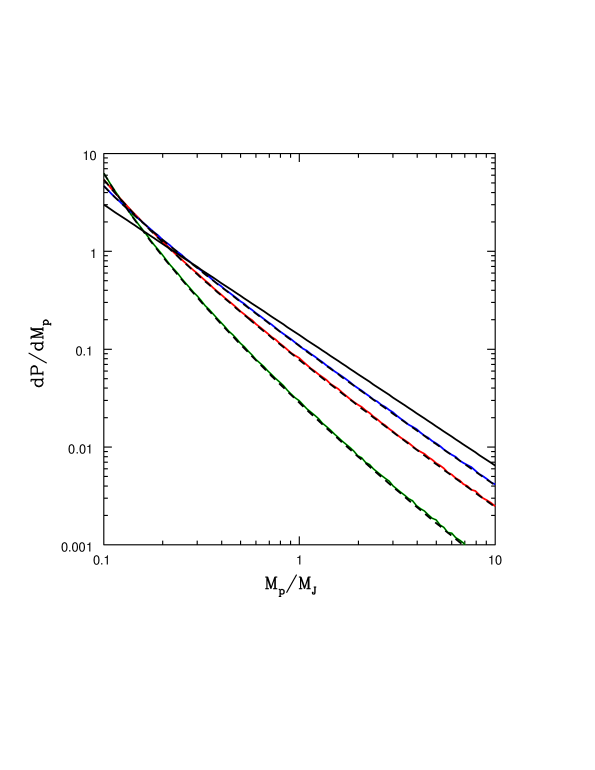
Figure 1: Planetary Mass Function. The curves show the planetary mass function predicted from an exponential distribution of disk lifetimes and a uniform-random distribution of mass accretion rates. The distributions are characterized by the mass scale $M_{0}$, which is determined by the the overall mass accretion rate ${\dot{M}}_{0}$ and the time scale $\tau$ of the disk lifetime distribution. Results are shown for $M_{0}=1M_{J}$ (green) $\sqrt{10}M_{J}$ (red), and $10M_{J}$ (blue). For each case, the colored curves are determined by sampling from the distributions, whereas the underlying dashed black curves show the analytic result from equation (18). For comparison, the solid black curve shows a power-law mass distribution ($dP/dM\sim M^{-1.3}$).

Given the above results, we can construct planetary mass functions in two ways: First, we can sample the variables in equation (15) using their specified distributions, calculate the masses, and construct the histogram of results. Second, we can use equation (18). Both results are shown in Figure 1 for different choices of the fiducial mass scale in the range $M_{0}$ = 1 – 10 $M_{J}$. The sampling results are shown as the colored curves and the analytic results are shown dashed black curves (note that the results are essentially the same). For comparison, the solid black curve shows the expected power-law mass function of the form $dF/dM\propto M^{-1.3}$. With low accretion rates (mass scale) $M_{0}=1M_{J}$ (green curve), the model produces a PMF that is steeper than the target distribution, with a deficit of high mass planets. For larger values of $M_{0}$, the theoretical PMF approaches a power-law form over most of the relevant mass range and is in reasonable agreement with the target distribution. Nonetheless, the theoretical distributions remain slightly steeper.

As mentioned above, the mass accretion rate from equation (14) is an increasing function of time. If the planet mass become sufficiently large, the predicted mass accretion rate becomes larger than the rate supplied by the circumstellar disk, so that the planetary mass accretion rate must saturate and approach a constant (maximum) value. The PMF here is constructed using the increasing form of the mass accretion rate. This assumption leads to somewhat larger planets for the tail of the distribution. For completeness, we also consider the opposite limit in Appendix A, where the mass accretion rate saturates and thus becomes constant while most of the planetary mass is acquired. This Appendix also illustrates how the PMF framework constructed in the paper can be modified or generalized.

4 Planetary Mass Functions for Varying Stellar Mass

The treatment thus far does not include the mass of the host star in the analysis. This section uses the observed properties of circumstellar disks, which depend on the mass of the star, to inform the models of the planetary mass function constructed in the previous section. Within this framework, the PMF is specified up to the characteristic mass scale $M_{0}$ defined in equation (19). Here we use the empirical scaling laws outlined in Section 2 to define how the mass scale $M_{0}$ varies as a function of the stellar mass, and use the result to specify the PMF for varying $M_{\ast}$.

Consider the accretion of gas onto a forming giant planet where the rate is a constant fraction $\epsilon$ of the disk accretion rate. Including the time dependence of the disk mass accretion rate from equation (7), the total mass accreted — and hence the mass of the planet — must be given by the integral

$$M_{\rm p}=\int_{t_{\rm onset}}^{t_{\rm end}}\epsilon{\dot{M}}_{d(0)}{m^{2}dt\over(1+t/t_{0})^{3/2}}=2\epsilon{\dot{M}}_{d(0)}t_{0}m^{2}\left[{1\over(1+t_{\rm onset}/t_{0})^{1/2}}-{1\over(1+t_{\rm end}/t_{0})^{1/2}}\right]\,,$$ (20)

where $m$ is the dimensionless stellar mass from equation (6). In order to define the characteristic mass scale $M_{0}$ as a function of $m$, we use the scaling laws from Section 2. The core formation time varies with stellar mass according to equation (8). The typical time for accretion to end is given by the disk lifetime parameter $\tau$, which varies with $m$ according to equation (5). We can then define the mass scale $M_{0}$ using the ansatz

$$M_{0}=\left[\epsilon{\dot{M}}_{d(0)}t_{0}\right]{\cal F}(m)\qquad{\rm where}\qquad{\cal F}(m)\equiv 2m^{2}\left[{1\over(1+\sqrt{m})^{1/2}}-{1\over(1+5/m)^{1/2}}\right]\,.$$ (21)

Notice that the function ${\cal F}(m)\to 0$ for stellar mass $m$ = $(\tau_{1}/t_{\rm c0})^{2/3}\sim 3$. Our interpretation of this finding is that relatively few planets should form in disks associated with larger stellar masses (see the discussion below).

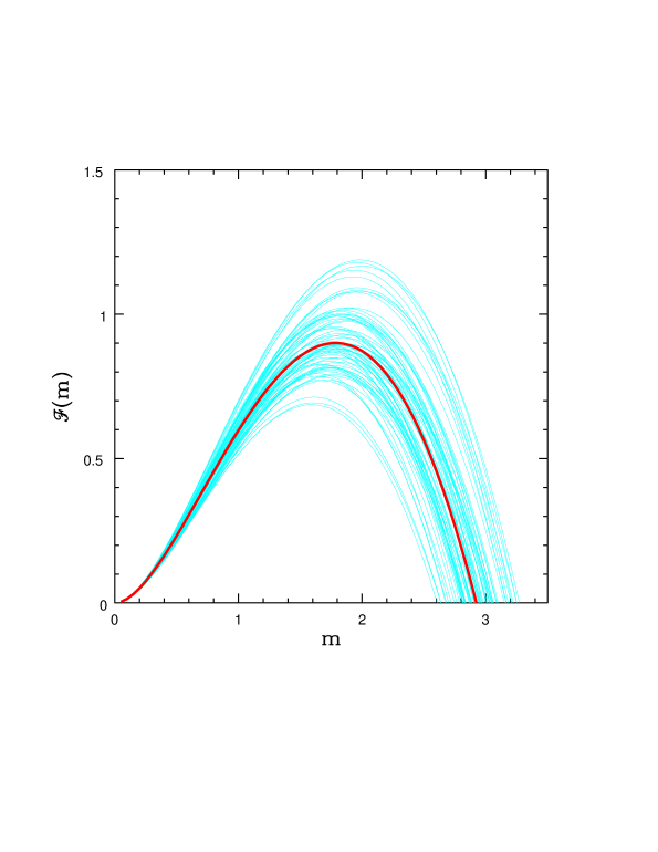
Figure 2: Relative mass fraction ${\cal F}(m)$ as a function of stellar mass, where $m=M_{\ast}/M_{\odot}$. The thick red curve shows the relative mass for typical values of the core formation time and disk lifetime, which are functions of stellar mass as outlined in the text. The collection of cyan curves shows the corresponding function where the baseline parameters $t_{\rm c0}$ and $\tau_{1}$ are allowed to vary with a (uniform) random distribution and an amplitude of 10 percent.

The relative mass fraction ${\cal F}(m)$ from equation (21) is shown in Figure 2 for standard values of the input parameters (solid red curve) and corresponding cases where the parameters are allowed to vary (lighter cyan curves). All of the curves follow the same basic trend: At low stellar masses, the accretion rate through the disk (${\dot{M}}\sim m^{2}$) becomes small, and this trend leads to small relative mass scales and hence the partial suppression of giant planet formation. In the opposite limit of large stellar mass, $m\sim 3$, the relative mass becomes small due to the lack of time for accretion. The time required for core formation becomes larger, while the disk lifetimes become shorter, so that little time is left for the cores (planets) to accrete gas. The observed scaling laws thus imply that larger stars ($m\,\raise 1.29167pt\hbox{$>$}\kern-7.5pt\lower 3.01385pt\hbox{$\sim$}\,3$) have difficulty producing giant planets via the core accretion paradigm. In the intermediate regime, for $m\sim 0.5-2$, the relative mass fraction varies (almost) linearly with increasing mass. This result suggests that distribution of companion mass ratios should be nearly the same for stars in this mass range. In constrast, the distribution should be steeper for stellar masses outside this range ($m\ll 0.5$ and/or $m\gg 2$).

For completeness, we can also evaluate the effects of stellar mass dependence in the limit where the disk mass accretion rate does not vary appreciably during the epoch when the planet accretes most of its mass. This limit corresponds to large values of the time scale $t_{0}$. One can show that in the limit of large $t_{0}$, the quantities from equation (21) become

$$M_{0}\equiv\epsilon{\dot{M}}_{d(0)}\tau_{1}\qquad{\rm and}\qquad{\cal F}(m)\equiv m\left[1-{t_{\rm c0}\over\tau_{1}}m^{3/2}\right]\,.$$ (22)

In this case, the function ${\cal F}(m)\to 0$ for stellar mass $m=(\tau_{1}/t_{\rm c0})^{2/3}$, which is the same as found above.

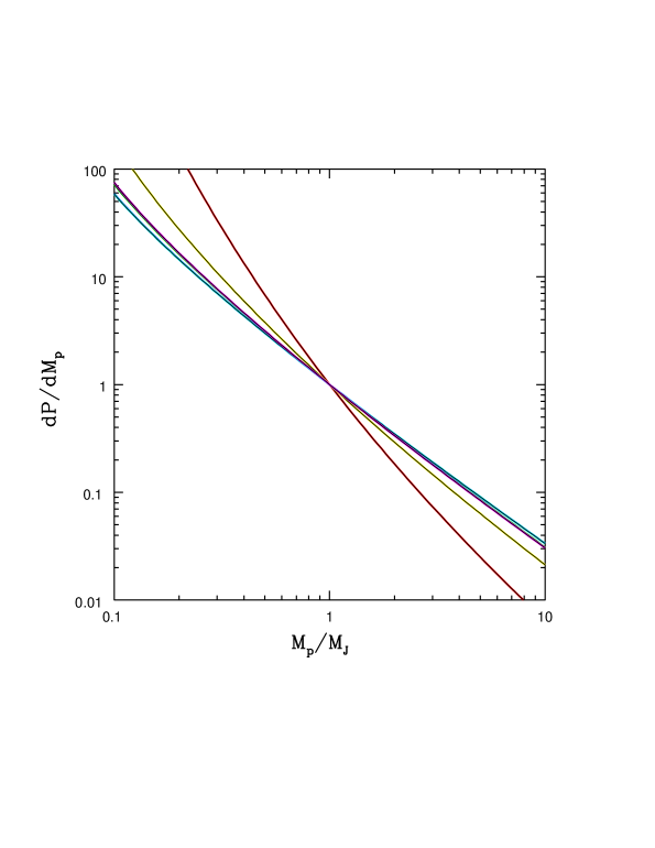
Figure 3: Planetary mass function for varying masses of the host star. The characteristic mass scale for the PMF is determined by the available mass supply, which depends on disk masses, accretion rates, and time scales according to equations (21) and (23). Curves are shown for stellar masses of $m$ = 0.25 (red), 0.5 (yellow), 1.0 (green), 1.5 (blue), 2.0 (cyan), and 2.5 (magenta). All of the mass distributions are normalized so that they are equal at $M_{\rm p}=M_{J}$.

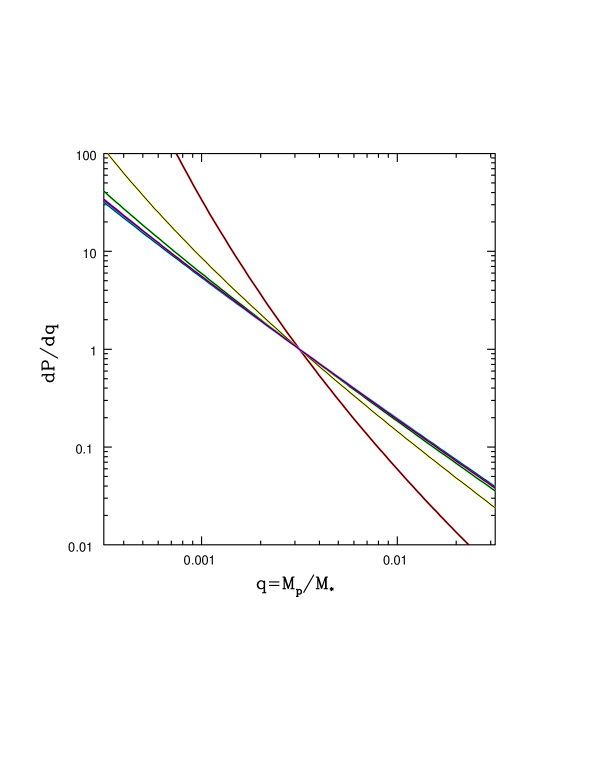
Figure 4: Planetary mass function expressed in terms of companion mass ratio $q=M_{\rm p}/M_{\ast}$ for varying masses of the host star. The mass scale $M_{0}$ for the PMF is determined by the available mass supply, which depends on disk masses, accretion rates, and time scales according to equations (21) and 23). Curves are shown for stellar masses of $m$ = 0.25 (red), 0.5 (yellow), 1.0 (green), 1.5 (blue), 2.0 (cyan), and 2.5 (magenta).

We can now construct the planetary mass function for different values of the stellar mass. The stellar mass dependence is incorporated by assuming that the total available mass for making a giant planet is proportional to the relative mass fraction ${\cal F}(m)$ defined above. For given stellar mass, the characteristic mass scale $M_{0}$ that determines the shape of the PMF is then taken to have the form

$$M_{0}={\cal F}(m)\times 5M_{J}\,.$$ (23)

Note that we are assuming that the mass scale for forming giant planets is proportional to the total mass available. However, since the disk can in principle form multiple planets, the coefficient in equation (23) is chosen to be only a fraction of the disk mass. If the mass scale $M_{0}$ is used in the PMF constructed according to Section 3, we obtain the distributions shown in Figure 3. The figure shows the mass functions for planets forming around stars with masses $m$ = 0.25 – 2.5. The planetary mass distributions for host stars in the range $m$ = 1 – 2.5 display a similar shape. In contrast, stars with lower masses show a significant deficit of larger planets, as shown by the PMF for $m=0.5$ (yellow curve) and especially that for $m=0.25$ (red curve). These steeper distributions imply that red dwarfs are less likely to have large planets, but are still expected have some Jovian companions (see also the more detailed planet formation models of Laughlin et al. 2004).

For even larger host stars, the available mass supply decreases due to the longer core formation times and shorter disk lifetimes (see Figure 2). Since ${\cal F}(m)\to 0$ for $m\,\raise 1.29167pt\hbox{$>$}\kern-7.5pt\lower 3.01385pt\hbox{$\sim$}\,3$, this present framework does not provide a mass distribution for planets around higher mass stars: such planets should be rare. This implication is roughly consistent with current observational results (Reffert et al., 2015), which find that the planet occurence rate drops significantly for stellar masses larger than $M_{\ast}\sim 2.5-3M_{\odot}$.

Emerging observational trends (Meyer et al., 2021) comparing low mass brown dwarf companions to gas giant planets, as a function of stellar mass, suggest that distributions of companion mass ratios are more universal than the distributions of companion masses themselves. In addition to the PMF, we thus consider the distribution of the mass ratios $q=M_{\rm p}/M_{\ast}$ in Figure 4 (for the same host star masses as before; compare with Figure 3). The resulting distributions of mass ratio are roughly similar across the range of stellar masses for $m\geq 0.5$. Once again, however, the distribution for stars with the smallest mass, $m=0.25$ (red curve), is steeper and shows a deficit of large-$q$ planets compared to the others. This deficit is due to the small fiducial mass scale, which results from the smaller available mass supply in the disks surrounding low mass stars. Although the curves are shown down to ratios $q=3\times 10^{-4}$ for all stellar masses, for $m=0.25$ this value corresponds to a planet with only $M_{\rm p}\sim 3$ $M_{\oplus}$. Planets with such small masses can accrete little gas, so that their production mechanism lies outside this framework for the formation of gas giants. Finally, we note that the similarity between the PMFs and the mass-ratio distributions (Figures 3 and 4) arises because the distributions have a nearly power-law form. In the limit where the PMF is exactly a power-law, the two distributions would have the same shape.

This finding has observational implications. Microlensing surveys measure companion mass ratios, and favor low mass stars (which are more common than larger stars). On the other hand, both RV and transit surveys have historically used our solar system as a template and favored solar-type stars. As a result, the observed distribution of companion mass ratios is predicted to be somewhat steeper for microlensing surveys than for the others. For the largest stellar mass considered here, $m=2.5$ (magenta curve), the PMF is nearly the same as for solar type stars, but even higher mass stars ($m>3$) should have relatively fewer large planets (because the relative mass fraction ${\cal F}\to 0$). Future observational work should determine how the distributions of planetary masses and mass ratios vary across the entire spectrum of stellar masses.

5 Conclusion

This paper constructs a series of models for the initial mass function for gas giant planets forming through the core accretion paradigm, including its dependence on the mass of the host star. This section provides a brief summary of our results (Section 5.1), followed by a discussion of their implications (Section 5.2).

5.1 Summary of Results

This paper develops a working framework for determining the planetary mass function within the core accretion paradigm. In this regime, the final planet mass is determined by its mass accretion history (see equation [1]). The treatment is semi-empirical in that the distributions of the input parameters are specified (in part) using observations of circumstellar disk properties. This approach can produce mass distributions that are roughly consistent with current observations over the mass range $M_{\rm p}=0.1-10M_{J}$ (e.g., see Figure 1).

Within current observational uncertainties, disk lifetimes are observed to be exponentially distributed, whereas the planetary mass function has a nearly power-law form. The framework developed in this paper produces a nearly power-law PMF using the exponential distribution of disk lifetimes as input. In order to obtain results consistent with observations, other input parameters — in addition to the disk lifetime — must sample distributions of values, and the mass accretion rate must increase as the planet grows. In the limiting case of a constant mass accretion rate, the exponential distribution of disk lifetimes imprints an exponential fall-off in the PMF, which leads to a deficit of larger planets compared to the observed distribution.

This analysis reveals an interesting feature for the expected case where the total disk lifetime has an exponential distribution: If we consider the time remaining after some initial temporal offset, for example after the planet reaches the stage where runaway gas accretion occurs, then the distribution of time remaining (after the offset) also has an exponential form (see equations [9 – 11]). Moreover, the exponential distribution has the same decay constant or half-life.

In this formulation of the problem, flow of material onto the planet is separated into two parts. The circumstellar disk provides a background reservoir of gas that ultimately supplies the forming planet. In general, disks support a (slow) radially inward mass accretion flow, and some fraction of this large-scale flux is intercepted by the planet, i.e., enters its sphere of influence as delineated by the Hill radius. In the vicinity of the planet, only a fraction of the incoming material is actually accreted by the planet. The overall efficiency of accretion onto the planet $\xi$, along with the disk lifetime $t$, vary from case to case and provide sufficient complexity to produce a nearly power-law PMF (Figure 1).

Disk properties — including lifetimes, mass accretion rates, and expected/inferred core formation times — are observed to vary with the mass $M_{\ast}$ of the host star. These variations imply that the total mass provided by the disk depends on stellar mass. In this approach, the fiducial mass scale $M_{0}$ for the PMF is assumed to scale with the relative mass fraction ${\cal F}$, thereby leading to planetary mass distributions that depend on $M_{\ast}$ (Section 4).

The PMFs constructed in this paper indicate that the probability of producing large planets around low mass stars is lower than for the case of solar-type stars, i.e., the PMF is steeper for small stars (Figure 3). This finding is consistent with observational surveys (Bonfils et al., 2013; Vigan et al., 2020) as well as theoretical expectations (Laughlin et al., 2004)). On the other hand, for sufficiently massive stars, with $M_{\ast}\,\raise 1.29167pt\hbox{$>$}\kern-7.5pt\lower 3.01385pt\hbox{$\sim$}\,3M_{\odot}$, the core formation time scales become comparable to typical disk lifetimes, and the probability of producing giant planets is reduced (Figure 2; see also Reffert et al. 2015). If we consider the distribution of mass ratios $q=M_{\rm p}/M_{\ast}$, instead of the PMF itself, the resulting distributions are roughly similar across the range of intermediate stellar masses $M_{\ast}=0.5-2.5M_{\odot}$ (Figure 4). However, the mass ratio distribution for low mass stars remains steeper than that for larger stars.

5.2 Discussion

This paper constructs models for the PMF using a combination of disk lifetimes and disk accretion properties. The microphysics of gas accretion onto forming planets provides additional degrees of freedom. Using the observed distribution of disk lifetimes and uniform distributions for efficiency parameters that describe the accretion processes, this framework can produce models that are roughly consistent with the observed PMF. In addition, apparent trends observed in the PMF for varying stellar mass can be reproduced. Given the current state of both observations and theory regarding the distribution of planetary masses, however, this work represents only a first step toward a complete understanding of the PMF. Many issues should be addressed in greater detail.

The current version of the theory is incomplete. For example, this paper accounts for the accretion history of gas flow onto forming planets in a parametric manner, including the introduction of efficiency factors. As the process of disk accretion becomes better understood (Hartmann, 2009; Zhu et al., 2011; Szulágyi et al., 2017), the fundamentals of disk physics should be incorporated into the models, ultimately leading to specific probability distributions for the input variables. Another complication is that several mechanisms can act to stop (or at least slow down) accretion onto forming planets. These processes include gap opening in the circumstellar disks, the effects of the rotating reference frame on accretion onto the planet surface, repulsion of the accretion flow by magnetic fields, and the physics of accretion within the circumplanetary disk. This current treatment also ignores planetary migration, which can induce variations in the accretion rate as the planets change their orbital elements (particularly if accretion rates vary with radial location). In addition, disks often produce multi-planet systems, and the effects of additional bodies can influence the formation of their neighbors. All of these effects should be integrated into future studies.

The models considered here are relatively simple, in that they involve only the disk lifetime $t$, an accretion efficiency factor $\xi$, and the manner in which accretion scales with planetary mass. As the number of physical processes contributing to the determination of planet mass increases, thereby including more variables that sample distributions of values, the resulting PMF departs further from the functional forms of the individual distributions. In the limit where the number of independent contributing variables is large, the central limit theorem comes into play, and the resulting PMF approaches a log-normal form (e.g, Richtmyer 1978). Since the observed PMF is approximately a power-law, this feature argues for an intermediate number of relevant (and independent) variables. The process is not completely scale-free, however, and one should keep in mind that the power-law form of the PMF only manifests itself over a limited range of parameter space.

The theoretical framework of this paper highlights two observational issues that are important for understanding the PMF — the distribution of disk lifetimes for ages $t\sim 10$ Myr and the distribution of planetary masses for $M_{\rm p}\sim 10M_{J}$. The characteristic mass scale $M_{0}$ is important for determining the shape of the PMF (see equation [19]), which depends on the time scale $\tau$ appearing in the distribution of disk lifetimes. Specification of the scale $\tau$ determines the fraction of ‘long-lived’ disks, which in turn determines the probability of producing large planets with $M_{\rm p}\sim 10M_{J}$. As a result, it will be useful for observations to measure the fraction of disks that live for $\sim 10$ Myr (Thanathibodee et al., 2018). If the value of the mass scale $M_{0}$ is small (e.g., due to a small time scale $\tau$), the formation of large planets is suppressed. The degree of suppression, in turn, affects the apparent slope of the PMF for planets more massive than Jupiter. The observational determination of the planetary mass function for masses $M_{\rm p}\sim 10M_{J}$ is thus crucial for testing the PMF produced by the core accretion paradigm (although such observations will be challenging).

In addition to the core accretion paradigm, some planets could be produced through gravitational instability in sufficiently massive disks (see, e.g., Boss 1997 to Wagner et al. 2019). These planets tend to have larger masses $M_{\rm p}\sim 10M_{J}$ (see, e.g., Adams & Benz 1992 to Stamatellos & Inutsuka 2018) and could thus contribute to the planetary mass function at the high-mass end. The results of this paper suggest that the exponential distribution of disk lifetimes can cause the core accretion paradigm to underproduce high mass planets, so that additional planets produced via gravitational instability could fill this gap. Notice also the brown dwarf binaries can contribute to the ‘planetary’ mass distribution for $M_{\rm p}\sim 10M_{J}$ (Meyer et al., 2021).

As outlined above, gravitational instability tends to produce more massive planets, and they tend to form with large semi-major axes (e.g., Rafikov 2005; see Vigan et al. 2017 for current observational constraints). In contrast, the observed populations of Hot Jupiters and more temperate gas giants tend to have smaller masses then their colder counterparts (e.g., Howard et al. 2010). As a result, future studies (both observational and theoretical) should determine the PMF for different ranges of orbital separations.

Finally, we note that theoretical descriptions of the planetary mass function suffer from a lack of uniqueness. An intrinsic aspect of the problem is that many physical processes contribute to the PMF, so that the distributions of many input variables combine to produce a single function. As a result, although the models of this paper successfully reproduce the nearly power-law form of the PMF that is observed, alternate approaches could also work. Fortunately, the framework developed here is more robust than this initial application, so that future studies can improve the various steps of the calculation.

  Acknowledgment: We would like to thank Veenu Seri for early work that helped formulate the problem. We also thank Konstantin Batygin, Nuria Calvet, and Greg Laughlin for many useful discussions, and thank the referees for their comments on the manuscript. This work was supported by the University of Michigan, the NASA JWST NIRCam project (contract number NAS5-02105), and the NASA Exoplanets Research Program (grant number NNX16AB47G).

Appendix A Planetary Mass Function for Constant Accretion Rate

In this Appendix, consider the limiting case where the mass accretion rate onto the planet approaches a constant and calculate the corresponding PMF. In this context, the planetary mass $M_{\rm p}$ is given by

$$M_{\rm p}=M_{\scriptstyle I\!I}+{\dot{M}}_{0}\xi t=M_{\scriptstyle I\!I}+M\,,$$ (A1)

where $t$ is the disk life time, $\xi$ is a uniform-random variable as before, and the mass accretion rate ${\dot{M}}_{0}$ is constant. The second equality defines the mass $M$ accreted after the onset of rapid accretion.

The distribution of the mass $M$ is determined by the cummulative probability

$$P(m<M)=\int_{0}^{t_{\ast}}{dt\over\tau}\exp[-t/\tau]+\int_{0}^{t_{\ast}}{dt\over\tau}\exp[-t/\tau]{t_{\ast}\over t}\,,$$ (A2)

where the time scale $t_{\ast}$ is defined by

$$t_{\ast}=M/{\dot{M}}_{0}\,.$$ (A3)

The probability distribution function for the accreted mass $M$ thus takes the form

$${dP\over dM}={1\over{\dot{M}}_{0}\tau}E_{1}\left({M\over{\dot{M}}_{0}\tau}\right)={1\over M_{0}}E_{1}\left({M\over M_{0}}\right)\,,$$ (A4)

where the second equality defines $M_{0}={\dot{M}}_{0}\tau$. If the starting mass $M_{\scriptstyle I\!I}$ is constant, then the corresponding probability distribution for the planetary mass $M_{\rm p}$ has the form

$${dP\over dM_{\rm p}}={1\over M_{0}}E_{1}\left({M_{\rm p}-M_{\scriptstyle I\!I}\over M_{0}}\right)\,.$$ (A5)

References

- Abramowitz & Stegun (1972) Abramowitz, M., & Stegun, I. A. 1972, Handbook of Mathematical Functions (New York: Dover)
- Adams & Benz (1992) Adams, F. C., & Benz, W. 1992, in ASP Conf. Proc. 32, Complementary Approaches to Double and Multiple Star Research, ed. H. A. McAlister & W. I. Hartkopf (San Francisco: ASP), 185
- Adams & Fatuzzo (1996) Adams, F. C., & Fatuzzo, M. 1996, ApJ, 464, 256
- Andrews et al. (2009) Andrews, S. M., Wilner, D. J., Hughes, A. M., Qi, C., & Dullemond, C. P. 2009, ApJ, 700, 1502
- Andrews et al. (2013) Andrews, S. M., Rosenfeld, K. A., Kraus, A. L., & Wilner, D. J. 2013, ApJ, 771, 129
- Ansdell et al. (2016) Ansdell, M., Williams, J. P., van der Marel, N. et al. 2016, ApJ, 828, 46
- Batalha et al. (2011) Batalha, N. M., Borucki, W. J., Bryson, S. T., et al. 2011, ApJ, 729, 27
- Barenfeld et al. (2016) Barenfeld, S. A., Carpenter, J. M., Ricci, L., & Isella, A. 2016, ApJ, 827, 142
- Batygin (2018) Batygin, K. 2018, AJ, 155, 178
- Benz et al. (2014) Benz, W., Ida, S., Alibert, Y., Lin, D., & Mordasini, C. 2014, in Protostars and Planets VI, ed. H. Beuther et al. (Tucson, AZ: Univ. Arizona Press), 691
- Bitsch et al. (2015) Bitsch, B., Lambrechts, M., & Johansen, A. 2015, A&A, 582, 112
- Bonfils et al. (2013) Bonfils, X., Delfosse, X., Udry, S., Forveille, T., Mayor, M., Perrier, C., Bouchy, F., Gillon, M., Lovis, C., Pepe, F., Queloz, D., Santos, N. C., Ségransan, D., & Bertaux, J.-L. 2013, A&A, 549, 109
- Borucki et al. (2010) Borucki, W. J., Koch, D., Basri, G., et al. 2010, Sci, 327, 977
- Boss (1997) Boss, A. P. 1997, Science, 276, 1836
- Carpenter et al. (2006) Carpenter, J. M., Mamajek, E. E., Hillenbrand, L. A., & Meyer, M. R. 2006, ApJ, 651, L49
- Carrera et al. (2018) Carrera, D., Davies, M. B., & Johansen, A. 2018, MNRAS, 478, 961
- Chambers (2016) Chambers, J. E. 2016, ApJ, 825, 63
- Cridland (2018) Cridland, A. J. 2018, A&A, 619, 165
- Cumming et al. (2008) Cumming, A., Butler, R. P., Marcy, G. W., Vogt, S. S., Wright, J. T., & Fischer, D. A. 2008, PASP, 120, 531
- Dullemond et al. (2006) Dullemond, C., Natta, A., & Testi, L. 2006, ApJ, 645, 69
- Dürmann & Kley (2017) Dürmann, C., & Kley, W. 2017, A&A, 598, A80
- Eisner et al. (2018) Eisner, J. A., Arce, H. G., Ballering, N. P. et al. 2018, ApJ, 860, 77
- Fedele et al. (2010) Fedele, D., van den Ancker, M. E., Henning, T., Jayawardhana, R., & Oliveira, J. M. 2010, A&A, 510, A72
- Fulton et al. (2017) Fulton, B. J., Petigura, E. A., Howard, A. W., et al. 2017, AJ, 154, 109
- Fung et al. (2019) Fung, J., Zhu, Z., & Chiang E. 2019, ApJ, 887, 152
- Gaudi et al. (2020) Gaudi, S. B., Christiansen, J. L., & Meyer, M. R. 2020, in ExoFrontiers: Big questions in exoplanetary science, Ed. N Madhusudhan (Bristol: IOP Publishing Ltd), arXiv:2011.04703
- Ginzburg & Chiang (2019) Ginzburg, S., & Chiang E. 2019, MNRAS, 487. 681
- Gullbring et al. (1998) Gullbring, E., Hartmann, L, Briceño, C., & Calvet, N. 1998, ApJ, 492, 323
- Haisch et al. (2001) Haisch, K.E., Lada, E.A., & Lada, C.J. 2001, ApJ, 553, L153
- Han et al. (2014) Han, E., Wang, S., Wright, J., et al. 2014, PASP, 126, 827
- Hansen & Kawaler (1994) Hansen, C. J., & Kawaler, S. D. 1994, Stellar Structure and Evolution (Springer)
- Hansen & Murray (2013) Hansen, B.M.S., & Murray, N. 2013, ApJ, 775, 53
- Hartmann (2006) Hartmann, L., D’Alessio, P., Calvet, N., & Muzerolle, J. 2006, ApJ, 648, 484
- Hartmann (2009) Hartmann, L. W. 2009, Accretion Processes in Star Formation (Cambridge: Cambridge Univ. Press)
- Hartmann et al. (2016) Hartmann, L., Herczeg, G., & Calvet, N. 2016, ARA&A, 54, 135
- Helled et al. (2014) Helled, R., Bodenheimer, P., Podolak, M., Boley, A., Meru, F., Nayakshin, S., Fortney, J. J., Mayer, L., Alibert, Y., & Boss, A. P. 2014, in Protostars and Planets VI, ed. H. Beuther et al. (Tucson, AZ: Univ. Arizona Press), 643
- Hernández et al. (2007) Hernández, J., Hartmann, L., Megeath, M. et al. 2007, ApJ, 662, 1067
- Hillenbrand et al. (1998) Hillenbrand, L. A., Strom, S. E., Calvet, N. et al. 1998, AJ, 116, 1816
- Howard et al. (2010) Howard, A. W., Marcy, G. W., Johnson, J. A. 2010, Science, 330, 653
- Ida & Lin (2008) Ida, S., & Lin, D.N.C. 2008, ApJ, 685, 584
- Jefferys (1939) Jeffreys, H. 1939, Theory of Probability (Clarendon Press)
- Lambrechts & Johansen (2012) Lambrechts, M., & Johansen, A. 2012, A&A, 544, 32
- Lambrechts & Johansen (2014) Lambrechts, M., & Johansen, A. 2014, A&A, 572, 107
- Laughlin et al. (2004) Laughlin, G., Bodenheimer, P., & Adams, F. C. 2004, ApJ, 612, L73
- Lee (2019) Lee, E. J. 2019, ApJ, 878, 36
- Lin et al. (2018) Lin J. W., Lee E. J., & Chiang E. 2018, MNRAS, 480, 4338
- Machida et al. (2008) Machida, M. N., Kokubo, E., Inutsuka, S., & Matsumoto, T. 2008, ApJ, 685, 1220
- Malhotra (2015) Malhotra, R. 2015, ApJ, 808, 71
- Malik et al. (2015) Malik, M., Meru, F., Mayer, L., & Meyer, M. 2015, ApJ, 802, 56
- Mamajek (2009) Mamajek, E. E. 2009, in AIP Conference Series 1158, Exoplanets and Disks, eds. T. Usuda, M. Tamura, & M. Ishii (Melville, NY: AIP), 3
- Manzo-Martínez et al. (2020) Manzo-Martínez, E., Calvet, N., Hernández, J., Lizano, S., Hernández, R. F., Miller, C. J., Maucó, K., Briceo, C., & D’Alessio, P. 2020, ApJ, 893, 56
- Mayor et al. (2011) Mayor, M., Marmier, M., Lovis, C., Udry, S., Ségransan, D., Pepe, F., Benz, W., Bertaux, J.-L., Bouchy, F., Dumusque, X., Lo Curto, G., Mordasini, C., Queloz, D., & Santos, N. C. 2011, arXiv:1109.2497
- Meyer et al. (2007) Meyer, M. R., Backman, D. E., Weinberger, A. J., & Wyatt, M. C. 2007, in Protostars and Planets V, ed. B. Reipurth, D. Jewitt, & K. Keil (Tucson, AZ: Univ. Arizona Press), 573
- Meyer et al. (2021) Meyer, M. R., Amara, A., Susemiehl, N., & Peterson, A. 2020, AAS Journals, in preparation
- Mordasini et al. (2009) Mordasini, C., Alibert, Y., & Benz, W. 2009, A&A, 501, 1139
- Natta et al. (2007) Natta, A., Testi, L., Calvet, N., Henning, Th., Waters, R., & Wilner, D. 2007, in Protostars and Planets V, ed. B. Reipurth, D. Jewitt, & K. Keil (Tucson, AZ: Univ. Arizona Press), 767
- Nielsen et al. (2019) Nielsen, E. L., De Rosa, R. J., Macintosh, B. et al. 2019, AJ, 158, 13
- Ormel & Klahr (2010) Ormel, C. W. & Klahr, H. H. 2010, A&A, 520, 43
- Ormel (2017) Ormel, C. W. 2017, Astrophysics and Space Science Library, 445, 197
- Otegi et al. (2020) Otegi, J. F., Bouchy, F., & Helled, R. 2020, A&A, 634, 43
- Pascucci et al. (2016) Pascucci, I., Testi, L., Herczeg, G. J., et al. 2016, ApJ, 831, 125
- Pascucci et al. (2018) Pascucci, I., Mulders, G. D., Gould, A., & Fernandes, R. 2018, ApJ, 856, L28
- Paxton et al. (2011) Paxton, B., Bildsten, L., Dotter, A. et al. 2011, ApJ Suppl., 192, 3
- Piso et al. (2015) Piso A.-M. A., Youdin A. N., & Murray-Clay R. A., 2015, ApJ, 800, 82
- Pollack et al. (1996) Pollack, J. B., Hubickyj, O., Bodenheimer, P., Lissauer, J. J., Podolak, M., & Greenzweig, Y. 1996, Icarus, 124, 62
- Rafikov (2005) Rafikov, R. R. 2005, ApJ, 621, L69
- Reffert et al. (2015) Reffert, S. Bergmann, C., Quirrenbach, A., Trifonov, T., & Künstler, A. 2015, A&A, 574, 116
- Ribas et al. (2015) Ribas, Á., Bouy, H., & Merín, B. 2015, A&A, 576, 52
- Richtmyer (1978) Richtmyer, R. D. 1978, Principles of Advanced Mathematical Physics (New York: Springer-Verlag)
- Rosenthal et al. (2018) Rosenthal, M. M., Murray-Clay, R. A., Perets, H. B., & Wolansky, N. 2018, ApJ, 861, 74
- Safronov (1977) Safronov, V. S. 1977, NASSP, 370, 797
- Safronov & Zvjagina (1969) Safronov, V. S., & Zvjagina, E. V. 1969, Icarus, 10, 109
- Salpeter (1955) Salpeter, E. E. 1955, ApJ, 121, 161
- Schlaufman (2015) Schlaufman, K. C. 2015, ApJ, 799, L26
- Schlaufman (2018) Schlaufman, K. C. 2018, ApJ, 853, 37
- Shvartzvald et al. (2016) Shvartzvald, Y., Maoz, D., Udalski, A., et al. 2016, MNRAS, 457, 4089
- Stamatellos & Inutsuka (2018) Stamatellos D., & Inutsuka S.-I., 2018, MNRAS, 477, 3110
- Suzuki et al. (2016) Suzuki, D., Bennett, D. P., Sumi, T., et al. 2016, ApJ, 833, 145
- Suzuki et al. (2018) Suzuki, D., Bennett, D. P., Ida, S. et al. 2018, ApJL, 869, L34
- Szulágyi et al. (2017) Szulágyi, J. 2017, ApJ, 842, 103
- Tanigawa & Tanaka (2016) Tanigawa, T., & Tanaka, H. 2016, ApJ, 823, 48
- Tanigawa & Watanabe (2002) Tanigawa, T., & Watanabe, S.-I. 2002, ApJ, 580, 506
- Thanathibodee et al. (2018) Thanathibodee, T., Calvet, N., & Herczeg, G. 2018, ApJ, 861, 73
- Thommes et al. (2008) Thommes, E. W., Matsumura, S., & Rasio, F. A. 2008, Science, 321, 814
- Vigan et al. (2017) Vigan, A., Bonavita, M., Biller, B. et al. 2017, A&A, 603, 3
- Vigan et al. (2020) Vigan, A., Fontanive, C., Meyer, M. et al. 2020, A&A, submitted, arXiv:2007.06573
- Wagner et al. (2019) Wagner, K., Apai, D., & Kratter, K. M. 2019, ApJ, 877, 46
- Williams & Cieza (2011) Williams, J. P., & Cieza, L. A. 2011, ARA&A, 49, 67
- Winn & Fabrycky (2015) Winn, J. N., & Fabrycky, D. C. 2015, ARA&A, 53, 409
- Wolfgang et al. (2016) Wolfgang, A., Rogers, L. A., & Ford, E. B. 2016, ApJ, 825, 19
- Yao et al. (2018) Yao, Y., Meyer, M. R., Covey, K. R., Tan, J. C., & Da Rio, N. 2018, ApJ, 869, 72
- Yasui (2014) Yasui, C., Kobayashi, N., Tokunaga, A. T., & Saito, M. 2014, MNRAS, 442, 2543
- Zhu et al. (2018) Zhu, W., Petrovich, C., Wu, Y., Dong., S., & Xie, J. 2018, ApJ, 860, 101
- Zhu et al. (2011) Zhu, Z., Nelson, R. P., Hartmann, L., Espaillat, C., & Calvet, N., 2011, ApJ, 729, 47