Fourier, Gabor, Morlet or Wigner:
Comparison of Time-Frequency Transforms

Abstract

In digital signal processing time-frequency transforms are used to analyze time-varying signals with respect to their spectral contents over time. Apart from the commonly used short-time Fourier transform, other methods exist in literature, such as the Wavelet, Stockwell or Wigner-Ville transform. Consequently, engineers working on digital signal processing tasks are often faced with the question which transform is appropriate for a specific application. To address this question, this paper first briefly introduces the different transforms. Then it compares them with respect to the achievable resolution in time and frequency and possible artifacts. Finally, the paper contains a gallery of time-frequency representations of numerous signals from different fields of applications to allow for visual comparison.

I Introduction

In many fields of engineering and science it is vital to analyze the spectral content of time-varying signals as it changes over time. This includes medical signals (EEG, ECG, ultrasonic), music and speech, animal voices, seismic activity, vibrations, fluctuations in power grids, radar and communication signals and many more.

For that purpose many different types of time-frequency transforms have been introduced in literature. Some of the transforms have a high practical impact, others are more of theoretical interest. The available methods provide largely different properties such as time resolution, frequency resolution, accuracy and the potential introduction of artifacts that do not correspondent to actual signal components.

This paper considers the STFT, Gabor, Wavelet and Stockwell (S) transform as well as the Wigner-Ville distribution (WVD) and its smoothed pseudo variant (SPWVD). Section II provides a brief introduction to these methods. Readers that are interested in more in-depth information and the theoretical backgrounds are referred to [1, 2, 3]. Section III compares the transforms with respect to resolution and artifacts. Finally, the transforms are applied to numerous different signals to form a gallery of time-frequency transforms. The purpose of this gallery is to show the properties, advantages and disadvantages of the transforms on actual signals in order to support engineers selecting the right transform for their application.

II Time-Frequency Transforms

II-A Short-Time Fourier and Gabor Transform

The STFT is the most widely known and commonly used time-frequency transform. It is well understood, easy to interpret and there exist fast implementations (FFT). Its drawbacks are the limited and fixed resolution in time and frequency.

The idea of the STFT is to move a sliding window $w(t)$ over the signal $x(t)$ to be analyzed, such that a particular time span of the signal is selected. For each position of the window a Fourier transform is calculated, that represents the frequency content of that time span. The STFT results in the two dimensional time-frequency representation:

$$X(t,f)=\intop_{-\infty}^{\infty}x(t_{1})w^{*}(t_{1}-t)e^{-j2\pi ft_{1}}dt_{1}$$

For spectral analysis the squared magnitude of the STFT is considered, which is called spectrogram:

$$S_{x}(t,f)=\left|X(t,f)\right|^{2}$$

Time and frequency resolution can be controlled by the window length, as shown in Figures 2 and 3: A short window captures only a short period of time and has thus a precise time resolution. However, the frequency resolution is poor, because the windowed signal contains only few time samples resulting in only few frequency bins. Contrary, a long window provides poor time resolution, but creates precise frequency information due to the larger number of samples. This phenomenon is known as the uncertainty principle, that states that the product of resolution in time and frequency is limited: $BT\geq\frac{1}{4\pi}$ (with B being the bandwidth of one frequency bin) [2].

A special case of the STFT, where the uncertainty equation above is fulfilled with equality (i.e. having the best joint time and frequency resolution), is known as the Gabor transform. The Gabor transform is simply a STFT with the window being a Gaussian function

$$w(t)=e^{-\alpha t^{2}}$$

where the parameter $\alpha$ controls the window length, i.e. the emphasis on time or frequency resolution.

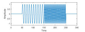
Figure 1: Exemplary signal in the time domain

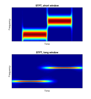
Figure 2: STFT (spectrogram) with short and long windows of the exemplary signal in Figure 1, showing the difference in frequency and time resolution

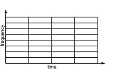
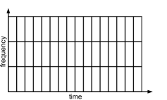
Figure 3: Resolution of the STFT with long (upper) and short window (lower)

II-B Wavelet Transform

The result of the wavelet transform differs from the STFT in that its time-frequency resolution is not fixed and depends on the frequency (multi-scale property, see Fig. 5). In general, the wavelet transform represents lower frequency components with finer frequency resolution and coarser time resolution. For higher frequencies the reverse is true: frequency resolution is coarser and time resolution is finer. This variable resolution property of the wavelet transform is sometimes superior to the Fourier approach, because it may give clearer spectral information for certain applications, such as audio signal processing.

The wavelet transform compares the time domain signal $x(t)$ with a short analysis function $\varPsi(t)$. $\varPsi(t)$ is called the wavelet and can take on many forms as will be described below. During the calculation of the transform the wavelet is repeatedly moved over the signal (time shifted) – each pass with a different scale factor in time, that dilates the wavelets to a different length (dilation or scale). This creates a two dimensional representation of time (i.e. shift) and scale (can be related to frequency). The time shift is denoted by $b$, the scale by $a$. The continuous wavelet transform (CWT) is defined as:

$$CWT(a,b)=\frac{1}{\sqrt{a}}\intop_{-\infty}^{\infty}x(t)\varPsi^{*}\left(\frac{t-b}{a}\right)dt$$

Analog to the spectrogram of the STFT, the scalogram of the wavelet transform is defined as

$$\left|CWT(a,b)\right|^{2}$$

Different wavelet functions are available for analysis. For the CWT commonly Morlet wavelets (also called Gabor wavelets) are used, that consist of a complex sine wave with Gaussian envelope

$$\varPsi_{Morlet}(t)=e^{-\alpha t^{2}}e^{j2\pi f_{c}t}$$

Here, the parameters “center frequency” $f_{c}$ and “width of Gaussian” $\alpha$ control the trade-off between time and frequency resolution and need to be selected before conducting the transform. Basically, wavelet functions need to be functions that are both local in time and frequency to provide adequate time and frequency resolution. Figure 4 shows an example of the scalogram of a CWT.

Note, that besides the CWT, the discrete wavelet transform (DWT) exists. Different from the CWT, the DWT preserves the complete information of the time domain signal and is thus invertible. Therefore the DWT is often used to create sparse signal representations that can be used for data compression (e.g. widely applied in image processing). Usually different types of wavelets are used for the DWT, such as the Haar or Daubechies wavelets. The DWT is often considered less suitable for time-frequency representation, because it creates less readable plots.

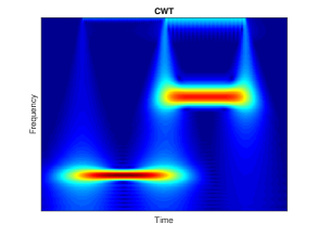
Figure 4: CWT (scalogram): note the varying resolution of frequency and time

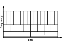
Figure 5: Variable resolution property of the CWT and S transform

II-C Stockwell Transform

The Stockwell or S-transform [4] is basically a STFT with a Gaussian (Gabor) window, whose length is frequency dependent. This results in a varying time-frequency resolution similar to the wavelet transform (Figure 5). The Stockwell transform is defined as

$$ST(t,f)=\intop_{-\infty}^{\infty}x(t_{1})\frac{\left|f\right|}{\sqrt{2\pi}}e^{\frac{-f^{2}(t_{1}-t)^{2}}{2}}e^{-j2\pi ft_{1}}dt_{1}$$

It is also similar to the CWT with a Morlet wavelet. However, in contrast to the CWT, the Stockwell transform has absolute referenced phase information. This means that the phase of the kernel functions, which are multiplied with the signal for analysis, at t = 0 is zero. Moreover, the Stockwell transform tends to emphasize higher frequency content due to the factor $|f|$ in its formula. Figure 6 shows an example.

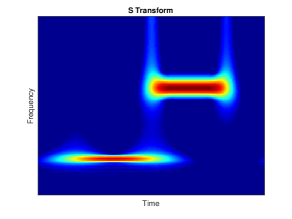
Figure 6: S transform: note the varying resolution of frequency and time and the emphasis on the higher frequency component

II-D Wigner-Ville Distribution

The Wigner-Ville distribution (WVD) [1] overcomes the limited resolution of the Fourier and wavelet based methods using an autocorrelation approach.

The standard version of the autocorrelation function (ACF) considers the pointwise multiplication of a signal with a lagged version of itself and integrates the results over time. It is defined as

$$r{}_{xx}(\tau)=\intop_{-\infty}^{\infty}x(t)x^{*}(t+\tau)dt$$

The standard ACF is only dependent on the lag $\tau$, because time is integrated out of the result. The WVD uses a variation of the ACF, called the instantaneous autocorrelation, which omits the integration step. Thus time remains in the result. The instantaneous autocorrelation is therefore a two dimensional function, depending on $t$ and the lag $\tau$:

$$R_{xx}(t,\tau)=x(t+\frac{\tau}{2})x^{*}(t-\frac{\tau}{2})$$

As an example, Figure 7 shows the instantaneous autocorrelation of a triangular shaped signal.

The WVD calculates the frequency content for each time step $t$ by taking a Fourier transform of the instantaneous autocorrelation across the axis of the lag variable $\tau$ for that given $t$ (depicted in Figure 7) :

$$W(t,f) = \intop_{-\infty}^{\infty}R_{xx}(t,\tau)e^{-j2\pi f\tau}d\tau$$

$$= \intop_{-\infty}^{\infty}x(t+\frac{\tau}{2})x^{*}(t-\frac{\tau}{2})e^{-j2\pi f\tau}d\tau$$

The result is real-valued. This way of calculation is related to the fact, that the Fourier spectrum of a signal equals the Fourier transform of its ACF.

The WVD offers very high resolution in both time and frequency, this is much finer than of the STFT.

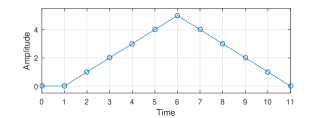
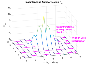
Figure 7: Depiction of the instantaneous autocorrelation $R_{xx}(t,\tau)$ and the calculation of the WVD of a triangular signal. The slices represent the pointwise multiplication of the signal with a lagged version of itself for a specific lag value $\tau$. Calculating a Fourier transform across the $\tau$-axis for every value of $t$ creates the WVD. If one would integrate over $t$ instead, the result would be the standard ACF.

An important disadvantage of the WVD are the so-called cross terms. These are artifacts occurring in the result, if the input signal contains a mixture of several signal components, see Figure 8. They stem from the fact, that the WVD is a quadratic (and therefore a non-linear) transform due to the way the instantaneous autocorrelation is calculated. The WVD of the superposition of two signals is

$$W{}_{x_{1}+x_{2}}=W{}_{x_{1}}+W{}_{x_{2}}+2\Re\left\{W_{x_{1},x_{2}}\right\}$$

and may be dominated by the cross term $W_{x_{1},x_{2}}$, which may have twice the amplitude of the auto terms $W{}_{x_{1}}$and $W{}_{x_{2}}$. Unfortunately, the occurrence of these cross terms limits the usefulness for many practical signals.

The WVD is usually calculated with the analytic version of the input signal that does not contain negative frequency components. This avoids cross terms between positive and negative frequency content that may mask low frequency components in the WVD.

The cross terms occur midway between the auto terms and often have an oscillatory (high-frequency) pattern. A method to reduce cross terms is to suppress the oscillating components by additional low-pass filtering in time and frequency. However, this suppression of cross terms comes at the expense of reduced resolution. This idea of additional cross term suppression leads to the more general formulation of time-frequency transforms called Cohen’s class [1, 3]. From Cohen’s class many different variants can be deduced, that basically differ in the way the low-pass filter is designed. A prominent one is the smoothed pseudo Wigner-Ville distribution (SPWVD) [3]. Other variants such as Choi-Williams, Margenau-Hill or Rihaczek can be found in literature, but often provide very similar results to the SPWVD for practical signals. The SPWVD is defined as the WVD filtered by two separate kernels $g(t)$ and $H(f)$ (need to be chosen prior to the transform), that smooth the WVD in frequency and time:

$$SPWVD(t,f)=\intop_{t_{1}}\intop_{f_{1}}g(t-t_{1})H(f-f_{1})W(t_{1,}f_{1})dt_{1}df_{1}$$

Figure 8 shows an example of the WVD and Figure 9 its smoothed version, the SPWVD.

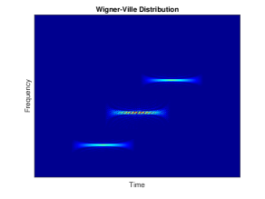
Figure 8: Wigner-Ville distribution: Cross term artifacts occur with high amplitude and oscillating behavior

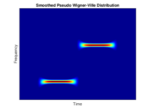
Figure 9: Smoothed pseudo WVD: cross terms are suppressed

III Comparison and Time-Frequency Gallery

The introduced time-frequency transforms are now compared with respect to their resolution in time and frequency. Figure 10 presents an overview of the schematic resolution grids. It visualizes the impact of the transforms and their parameters on the resolution. For completeness, the figure also shows the plain time domain and spectrum representations, that do not resolve frequency and time, respectively.

Furthermore, the transforms are compared for various synthetic signals and signals from real sources that cover different applications. The signals used for analysis consist of both synthetic and real-world signals. Synthetic signals include sweeps, pulses, frequency steps or short sine bursts. Some signals are composed of several of these elements. The results for synthetic signals are shown in Fig. Fourier, Gabor, Morlet or Wigner: Comparison of Time-Frequency Transforms and Fourier, Gabor, Morlet or Wigner: Comparison of Time-Frequency Transforms. Real-world signals include audio signals from speech and music (Fig. Fourier, Gabor, Morlet or Wigner: Comparison of Time-Frequency Transforms), radio signals with different modulation types (Fig. Fourier, Gabor, Morlet or Wigner: Comparison of Time-Frequency Transforms) and signals from nature and medical applications such as ECG, ultrasonic, bat sound, earthquake (Fig. Fourier, Gabor, Morlet or Wigner: Comparison of Time-Frequency Transforms).

The considered purpose of a transform is to visually present discriminative time and frequency features. Therefore only the magnitudes of the results are shown. Some transforms require certain parameters to be tuned, e.g. window length of the STFT or the center frequency of the Morlet mother wavelet. These parameters have been chosen such that the features of the signals become easily visible. According to common practice in literature, all transforms are typically plotted on linear frequency scale, except for the wavelet transform, which occurs both in logarithmic and linear scale.

Finally, the choice of the transform depends on the signal properties and the further use or subsequent processing of the results. Important aspects to consider are the desired resolution in time and frequency as well as the tolerability of artifacts. Table I summarizes the transforms and provides recommendations when to use which transform.

Transform	Time-Frequency Resolution	Artifacts	Application
Short-Time Fourier (STFT) / Gabor	poor	no	general purpose
Continuous Wavelet (CWT)	poor,
frequency dependent	no	when variable time-frequency resolution required, e.g. audio
Stockwell (S)	poor,
frequency dependent	no	when variable time-frequency resolution with a fixed phase alignment required, emphasizes higher frequencies
Smoothed Pseudo Wigner-Ville (SPWVD)	good	sometimes	general purpose, when high resolution required and some artifacts can be tolerated
Wigner-Ville (WVD)	excellent	strong	for simple signals or when artifacts can be tolerated

Table I: When to use which transform

Figure 10: Schematics of the resolutions of the transforms, including the time domain representation and the standard Fourier spectrum for comparison

Synthetic signals (1)

Synthetic signals (2)

Audio signals

Radio signals

Signals from nature and medical applications

References

- [1] J. Semmlow and B. Griffel, Biosignal and Medical Image Processing. CRC Press, 2014.
- [2] M. Sandsten, “Time-frequency analysis of time-varying signals and non-stationary processes,” Lund University, 2018.
- [3] F. Hlawatsch and G. F. Boudreaux-Bartels, “Linear and quadratic time-frequency signal representations,” IEEE Signal Processing Magazine, vol. 9, no. 2, pp. 21–67, 1992.
- [4] R. Stockwell, L. Mansinha, and R. Lowe, “Localization of the complex spectrum: the s transform,” IEEE Transactions on Signal Processing, 1996.