On the efficient parallel computing of long term reliable trajectories for the Lorenz system

Abstract

In this work we propose an efficient parallelization of multiple-precision Taylor series method with variable stepsize and fixed order. For given level of accuracy the optimal variable stepsize determines higher order of the method than in the case of optimal fixed stepsize. Although the used order of the method is greater then that in the case of fixed stepsize, and hence the computational work per step is greater, the reduced number of steps gives less overall work. Also the greater order of the method is beneficial in the sense that it increases the parallel efficiency. As a model problem we use the paradigmatic Lorenz system. With 256 CPU cores in Nestum cluster, Sofia, Bulgaria, we succeed to obtain a correct reference solution in the rather long time interval - [0,11000]. To get this solution we performed two large computations: one computation with 4566 decimal digits of precision and 5240-th order method, and second computation for verification - with 4778 decimal digits of precision and 5490-th order method.

Keywords: Parallel computing, Multiple precision, Variable stepsize Taylor series method, Lorenz system
Mathematics Subject Classification: 65L05, 65Y05

1 Introduction

Multiple precision Taylor series method is an affordable and very efficient numerical method for integration of some classes of low dimensional dynamical systems in the case of high precision demands Barrio1 ; Barrio2 . The method gives a new powerful tool for theoretical investigation of such systems.

A numerical procedure for computing reliable trajectories of chaotic systems, called Clean Numerical Simulation (CNS), is proposed by Shijun Liao in Liao1 and applied for different systems Liao2 ; CNS ; Li . The procedure is based on multiple precision Taylor series method. The main concept for CNS is the critical predictable time $T_{c}$, which is a kind of practical Lyapunov time. $T_{c}$ is defined as the time for decoupling of two trajectories computed by two different numerical schemes. The CNS works as follows. An optimal fixed stepsize is chosen. Then estimates of the required order of the method $N$ and the required precision (the number of exact decimal digits $K$ of the floating point numbers) are obtained. The optimal order $N$ is estimated by computing the $T_{c}-N$ dependence by means of the numerical solutions for fixed large enough $K$. The estimate of $K$ is obtained by computing the $T_{c}-K$ dependence by means of the numerical solutions for fixed large enough $N$. This estimate of $K$ is in fact an estimate for the Lyapunov exponent Wang . For given $T_{c}$ the solution is then computed with the estimated $N$ and $K$ and after that one more computation with higher $N$ and $K$ is performed for verification. The choice of $N$ and $K$ ensures that the round-off error and the truncation error are of the same order.

When very high precision and very long integration interval are needed, the computational problem can become pretty large. In this case the parallelization of the Taylor series method is an important task and needs to be carefully developed. The first parallelization of CNS is reported in par1 and later improved in par2 . A pretty long reference solution for the paradigmatic Lorenz system, namely in the time interval [0,10000], obtained in about 9 days and 5 hours by using the computational resource of 1200 CPU cores, is given in Liao3 . However, no details of the parallelization process are given in par1 ; par2 ; Liao3 . In our recent work Hybrid we reported in details a simple and efficient hybrid MPI+OpenMP parallelization of CNS for the Lorenz system and tested it for the same parameters as those in Liao3 . The results show very good efficiency and very good parallel performance scalability of our program.

This work can be regarded as a continuation of our previous work Hybrid , where fixed stepsize is used. Here we make a modification of CNS with a variable stepsize and fixed order following the simple approach given in Jorba . Although the used order of the method is greater then that in the case of fixed stepsize, and hence the computational work per step is greater, the reduced number of steps gives less overall work. Also the greater order of the method is beneficial in the sense that it increases the parallel efficiency. With 256 CPU cores in Nestum cluster, Sofia, Bulgaria, we succeed to obtain a correct reference solution in [0,11000] and in this way we improve the results from Liao3 . To obtain this solution we performed two large computations: one computation with 4566 decimal digits of precision and 5240-th order method, and second computation for verification - with 4778 decimal digits of precision and 5490-th order method for verification. The computations lasted $\approx$ 9 days and 18 hours and $\approx$ 11 days and 7 hours respectively. Let us note that the improvement of the numerical algorithm does not change the parallelization strategy from our previous work Hybrid , where the parallelization process is explained in more details. The difference from the previous parallel program is one additional OpenMP single section with negligible computational work, which computes the optimal step.

It is important to mention that although our test model is the classical Lorenz system, the proposed parallelization strategy is rather general - it could be applied as well to a large class of chaotic dynamical systems.

2 Taylor series method and CNS for the Lorenz system

We consider as a model problem the classical Lorenz system Lorenz :

$$\frac{dx}{dt} =\sigma(y-x)$$ (1)

$$\frac{dy}{dt} =Rx-y-xz$$

$$\frac{dz}{dt} =xy-bz,$$

where $R=28$, $\sigma=10$, $b=8/3$ are the standard Salztman’s parameters. For these parameters the system is chaotic. Let us denote with $x_{i},y_{i},z_{i},i=0,...,N$ the normalized derivatives (the derivatives divided by i!) of the approximate solution at the current time $t$. Then the N-th order Taylor series method for (1) with stepsize $\tau$ is:

$$x(t+\tau) \approx x_{0}+\sum_{i=1}^{N}x_{i}\tau^{i},$$ (2)

$$y(t+\tau) \approx y_{0}+\sum_{i=1}^{N}y_{i}\tau^{i},$$

$$z(t+\tau) \approx z_{0}+\sum_{i=1}^{N}z_{i}\tau^{i}.$$

The i-th Taylor coefficients (the normalized derivatives) are computed as follows. From system (1) we have

$$x_{1} =\sigma(y_{0}-x_{0}),$$

$$y_{1} =Rx_{0}-y_{0}-x_{0}z_{0},$$

$$z_{1} =x_{0}y_{0}-bz_{0}.$$

By applying the Leibniz rule for the derivatives of the product of two functions, we obtain the following recursive procedure for computing $x_{i+1},y_{i+1},z_{i+1}$ for $i=0,...,N-1$:

$$x_{i+1} =\frac{1}{i+1}\sigma(y_{i}-x_{i}),$$ (3)

$$y_{i+1} =\frac{1}{i+1}(Rx_{i}-y_{i}-\sum_{j=0}^{i}x_{i-j}z_{j}),$$

$$z_{i+1} =\frac{1}{i+1}(\sum_{j=0}^{i}x_{i-j}y_{j}-bz_{i}).$$

To compute the i+1-st coefficient in the Taylor series we need all previous coefficients from 0 to i. In fact, this algorithm for computing the coefficients of the Taylor series is called automatic differentiation, or sometimes algorithmic differentiation Moore . It is obvious that we need $O(N^{2})$ floating point operations for computing all coefficients. The subsequent evaluation of Taylor series with Horner’s rule needs only $O(N)$ operations.

Let us now explain how we choose the stepsize $\tau$. We use a variable stepsize strategy, which makes the method much more robust then in the fixed stepsize case. We use a simple strategy taken from Jorba , which ensures both the convergence of the Taylor series and the minimization of the computational work per unit time. If we denote the vector of the normalized derivatives of the solution with $\mathbf{X_{i}}=(x_{i},y_{i},z_{i})$ and take a safety factor 0.993, then the stepsize $\tau$ is determined by the last two terms of the Taylor expansions Jorba :

$$\tau=\frac{0.993}{e^{2}}\min\left\{{\left(\frac{1}{{\|\mathbf{X_{N-1}}\|}_{\infty}}\right)}^{\frac{1}{N-1}},{\left(\frac{1}{{\|\mathbf{X_{N}}\|}}_{\infty}\right)}^{\frac{1}{N}}\right\}$$ (4)

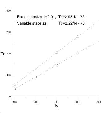
Figure 1: $Tc-N$ dependencies for fixed and variable stepsize

In Jorba the order of the method is determined by the local error tolerance. However, we do not work explicitly with some local error tolerance and also we do not use any explicit dependence between the local and the global error. Instead of this, as in Liao1 , we compute an a priori estimate of the needed order of the method for a reliable solution. As said before, the critical predictable time $T_{c}$ is defined as the time for decoupling of two trajectories computed by two different numerical schemes (in this case - by different $N$). The solutions are computed with large enough precision to ensure that the truncation error is the leading one. As a criterion for decoupling time we choose the time for establishing only 30 correct digits. The obtained $T_{c}-N$ dependencies for fixed stepsize $\tau=0.01$ and variable stepsize are shown in Figure 1. As seen from this figure, the computational work for one step in the case of variable stepsize is $\approx 80\%$ greater then in the case of fixed stepsize - ${(2.98/2.22)}^{2}\approx 1.80$. However, the reduced number of steps gives less overall work. Also the greater order of the method is beneficial in the sense that it increases the parallel efficiency. The reason is that with increasing the order $N$ of the method, the parallelizable part of the work becomes relatively even more larger than the serial part and the parallel overhead part.

Similarly, we compute an a priori estimate of the needed precision by means of computing the $T_{c}-K$ dependence. In this case we compare the solutions for different $K$ and large enough $N$. We obtain the dependence $T_{c}=2.55K-81$, which is the same, as expected, for fixed and for variable stepsize.

3 Parallelization of the algorithm

The improvement of the numerical algorithm does not change the parallelization strategy from our previous work Hybrid , where the parallelization process is explained in more details. However, as we will see, the variable stepsize not only decreases the computational work for a given accuracy, but also gives a higher parallel efficiency.

Let us store the Taylor coefficients in the arrays x, y, z of lengths N+1. The values of $x_{i}$ are stored in x[i], those of $y_{i}$ in y[i] and those of $z_{i}$ in z[i]. As explained in par1 ; par2 , the crucial decision for parallelization is to make a parallel reduction for the two sums in (3). However, in order to reduce the remaining serial part of the code and hence to improve the parallel speedup from the Amdal’s law, we should utilize some limited, but important parallelism. We compute x[i+1], y[i+1], z[i+1] in parallel. Moreover, we compute x[i+1] in advance, before computing the sums in (3), when during the reduction process some of the computational resource is free. In the same way we compute in advance Rx[i]-y[i] from the formula for y[i+1] and bz[i] from the formula for z[i+1]. These computations taken in advance matter, because multiplication is much more expensive then the other used operations (division by an integer number is not so expensive). The three evaluations by Horner’s rule for the new x[0], y[0], z[0] are also done in parallel.

In this work we consider a hybrid MPI+OpenMP strategy MPI ; OpenMP , i.e. every MPI process creates a team of OpenMP threads. For multiple precision floating point arithmetic we use GMP library (GNU Multiple Precision library) gnu . The main reason to consider a hybrid strategy, rather than a pure MPI one, is that OpenMP performs slightly better than MPI on one computational node. For packaging and unpackaging of the GMP multiple precision types for the MPI messages, we rely on the tiny MPIGMP library of Tomonori Kouya Kouya0 ; Kouya1 ; Kouya2 ; Kouya3 .

Figure 2: The sketch of hybrid MPI+OpenMP code in terms of GMP library.

It is important to note that for our problem the pure OpenMP parallelization has its own importance. First, the programming with OpenMP is easier because it avoids the usage of libraries like MPIGMP. Second, since the algorithm does not allow domain decomposition, the memory needed for one computational node is multiplied by the number of the MPI processes per that node, while OpenMP needs only one copy of the computational domain and thus some memory is saved.

The sketch of our parallel program is given in Figure 2. Every thread gets its id and stores it in tid and then the loop with index i is performed. Every MPI process takes its portion - the first and the last index controlled by the process. After that the directive #pragma omp for shares the work for the loop between threads.

Although OpenMP has a build-in reduction clause, we can not use it, because we use user-defined types for multiple precisions number and user-defined operations. A manual reduction by applying a standard tree based parallel reduction is done. We use containers for the partial sums of every thread and these containers are shared. The containers are stored in the array sum. We have in addition an array of temporary variables tempv for storing the intermediate results of the multiplications. To avoid false sharing, a padding strategy is applied OpenMP . At the point where each process has computed its partial sums, we perform MPI_ALLREDUCE between the master threadsMPI . It is useful to regard MPI_ALLREDUCE as a continuation of the tree based reduction process, which starts with the OpenMP reduction. Communications between master threads are overlapped with some computations for x[i+1], y[i+1], z[i+1] that can be taken before the computation of the sums in (3) is finished. When the MPI_ALLREDUCE is finished, we compute in parallel the remaining operations for x[i+1], y[i+1], z[i+1].

In between the block which computes the Taylor coefficients and the block which computes the new values of x[0], y[0], z[0] in parallel, we compute the new optimal stepsize within an omp single section. While the block for computing the Taylor coefficients is $O(N^{2})$ and the block for evaluations of the polynomials is $O(N)$, this block is only $O(1)$ and hence the work is negligible. Let us note that the GMP library does not offer a power function for the computations from formula (4). The good thing is that we do not need to compute the stepsize with multiple precision and double precision is enough. So we use the C standard library function pow in double precision. We do a normalization of the large GMP floating point numbers in order to work in the range of the standard double precision numbers. The C-code in terms of GMP library of our hybrid MPI+OpenMP program can be downloaded from radahpc .

Let us mention that if one half of the OpenMP threads computes one of the sums in (3) and the other half computes the other sum, one could also expect some small performance benefit, because for the small indexes i the unused threads will be less and also the difference from the perfect load balance between threads will be less. However, the last approach is not general because it strongly depends on the number of sums for reduction (two in the particular case of the Lorenz system) and the number of available threads.

4 Computational resources. Performance and numerical results.

The preparation of the parallel program and the many tests are performed in the Nestum Cluster, Sofia, Bulgaria nestum and in the HybriLIT Heterogeneous Platform at the Laboratory of IT of JINR, Dubna, Russia HybriLIT . The large computations for the reference solution in the time interval [0,11000] and the presented results for the performance are from Nestum Cluster. Nestum is a homogeneous HPC cluster based on two socket nodes. Each node consists of 2 x Intel(R) Xeon(R) Processor E5-2698v3 (Haswell-based processors) with 32 cores at 2.3 GHz. We have used Intel C++ compiler version 17.0, GMP library version 6.2.0, OpenMPI version 3.1.2 and compiler optimization options -O3 -xhost.

We use the same initial conditions as those in Liao3 , namely $x(0)=-15.8$, $y(0)=-17.48$, $z(0)=35.64$, in order to compare with the benchmark table in Liao3 . We computed a reference solution in the rather long time interval [0,11000] and repeated the benchmark table up to time 10000. Computing this table by two different stepsize strategies, is a good demonstration that Clean Numerical Simulation (CNS) is a correct and valuable approach for computing reliable trajectories of chaotic systems.

We performed two large computations with 256 CPU cores (8 nodes in Nestum). The first computation is with 4566 decimal digits of precision and 5240-th order method (5% reserve from the a priori estimates). The second computation is for verification - with 4778 decimal digits of precision and 5490-th order method (10% reserve from the a priori estimates). The first computation lasted $\approx$ 9 days and 18 hours and the second $\approx$ 11 days and 7 hours. The overall speedup with 256 cores for the first computation is 162.8, for the second - 164.6.

By estimating the time needed for the same accuracy and with fixed stepsize 0.01, we conclude that by applying variable stepsize strategy we have 2.1x speedup. There are two reasons for this speedup - less overall work and increased parallel efficiency. Although the work per step in the case of variable stepsize increases by $\approx 80\%$, the average stepsize is $\approx$ 0.034 and thus the overall work is $\approx 53\%$ from the work in the case of fixed stepsize 0.01. Also the parallel efficiency increases from 55.5% up to 63.6% for the first computation and from 56.2% up to 64.3% for the second. This is because by increasing the order of the method $N$, we increase the amount of the parallel work, which mitigates the impact of the serial work and the parallel overhead work.

As we compute the reference solution with some reserve of the estimated $N$ and $K$, we actually obtain the solution with some more correct digits. The reference solution with 60 correct digits at every 100 time units can be seen in radahpc . The reference solution at $t=11000$ is:

x= 6.10629269055689971917782003095370055267185885053970862735508

y=-3.33795350928712428173974978144552360814210542698512462640748

z= 34.1603471532583648867450334710712261840913307358242610005285

5 Conclusions

Parallelized version of multiple precision Taylor series method and particularly the Clean Numerical Simulation should be used with a variable stepsize strategy as a better alternative of the fixed stepsize one. An important observation is that variable stepsize not only decreases the computational work for a given accuracy, but also gives a higher parallel efficiency.

- (1) Barrio, Roberto. ”Performance of the Taylor series method for ODEs/DAEs.” Applied Mathematics and Computation 163.2 (2005): 525-545.
- (2) Barrio, Roberto, et al. ”Breaking the limits: the Taylor series method.” Applied mathematics and computation 217.20 (2011): 7940-7954.
- (3) Liao, Shijun. ”On the reliability of computed chaotic solutions of non-linear differential equations.” Tellus A: Dynamic Meteorology and Oceanography 61.4 (2008): 550-564
- (4) Liao, Shijun. ”On the numerical simulation of propagation of micro-level inherent uncertainty for chaotic dynamic systems.” Chaos, Solitons & Fractals 47 (2013): 1-12.
- (5) Liao, Shijun. ”On the clean numerical simulation (CNS) of chaotic dynamic systems.” Journal of Hydrodynamics, Ser. B 29.5 (2017): 729-747.
- (6) Li, Xiaoming, Yipeng Jing, and Shijun Liao. ”Over a thousand new periodic orbits of a planar three-body system with unequal masses.” Publications of the Astronomical Society of Japan 70.4 (2018): 64.
- (7) Wang, PengFei, and JianPing Li. ”On the relation between reliable computation time, float-point precision and the Lyapunov exponent in chaotic systems.” arXiv preprint arXiv:1410.4919 (2014).
- (8) Wang, Pengfei, Jianping Li, and Qian Li. ”Computational uncertainty and the application of a high-performance multiple precision scheme to obtaining the correct reference solution of Lorenz equations.” Numerical Algorithms 59.1 (2012): 147-159.
- (9) Wang, Pengfei, Yong Liu, and Jianping Li. ”Clean numerical simulation for some chaotic systems using the parallel multiple-precision Taylor scheme.” Chinese science bulletin 59.33 (2014): 4465-4472.
- (10) Liao, ShiJun, and PengFei Wang. ”On the mathematically reliable long-term simulation of chaotic solutions of Lorenz equation in the interval [0, 10000].” Science China Physics, Mechanics and Astronomy 57.2 (2014): 330-335.
- (11) Hristov, I., et al. ”Parallelizing multiple precision Taylor series method for integrating the Lorenz system.” arXiv preprint arXiv:2010.14993 (2020).
- (12) Jorba, Angel, and Maorong Zou. ”A software package for the numerical integration of ODEs by means of high-order Taylor methods.” Experimental Mathematics 14.1 (2005): 99-117.
- (13) Lorenz, Edward N. ”Deterministic nonperiodic flow.” Journal of the atmospheric sciences 20.2 (1963): 130-141.
- (14) Moore, Ramon E. Methods and applications of interval analysis. Society for Industrial and Applied Mathematics, 1979.
- (15) Gropp, William, et al. Using MPI: portable parallel programming with the message-passing interface. Vol. 1. MIT press, 1999.
- (16) Chapman, Barbara, Gabriele Jost, and Ruud Van Der Pas. Using OpenMP: portable shared memory parallel programming. Vol. 10. MIT press, 2008.
- (17) https://gmplib.org/
- (18) Kouya, Tomonori. ”BNCpack.” http://na-inet.jp/na/bnc/
- (19) Kouya, Tomonori. ”A Brief Introduction to MPIGMP & MPIBNCpack.”
- (20) Nikolaevskaya, Elena A., et al. ”MPIBNCpack library.” Studies in Computational Intelligence 397 (2012): 123-134.
- (21) Kouya, Tomonori. ”Performance Evaluation of Multiple Precision Numerical Computation using x86 64 Dualcore CPUs.” FCS2005 Poster Session (2005).
- (22) https://github.com/rgoranova/hpcvss
- (23) http://hpc-lab.sofiatech.bg/
- (24) http://hlit.jinr.ru/