A Framework of State-dependent Utility Optimization with General Benchmarks

Abstract

Benchmarks in the utility function have various interpretations, including performance guarantees and risk constraints in fund contracts and reference levels in cumulative prospect theory. In most literature, benchmarks are a deterministic constant or a fraction of the underlying wealth variable; thus, the utility is also a function of the wealth. In this paper, we propose a general framework of state-dependent utility optimization with stochastic benchmark variables, which includes stochastic reference levels as typical examples. We provide the optimal solution(s) and investigate the issues of well-definedness, feasibility, finiteness, and attainability. The major difficulties include: (i) various reasons for the non-existence of the Lagrange multiplier and corresponding results on the optimal solution; (ii) measurability issues of the concavification of a state-dependent utility and the selection of the optimal solutions. Finally, we show how to apply the framework to solve some constrained utility optimization problems with state-dependent performance and risk benchmarks as some nontrivial examples. Keywords: State-dependent utility optimization, General benchmarks, Non-existence of Lagrange multiplier, Measurability, Variational method MSC(2020): Primary: 49J55,  91B16; Secondary: 49K45, 91G80.JEL Classifications: G11, C61.

1 Introduction

Fix a probability space $(\Omega,\mathcal{F},\mathbb{P})$. The classical framework of expected utility maximization in portfolio selection (cf. Merton (1969)) is given by

$$\begin{split}\sup_{X}&~{}\mathbb{E}[u(X)]\\ \text{subject}\text{ to}&~{}\mathbb{E}[\xi X]\leqslant x_{0}\text{ and }u(X)>-\infty~{}\text{a.s.},\end{split}$$ (1)

where $X:\Omega\to\mathbb{R}$ is a random variable representing the wealth and $u:\mathcal{D}\rightarrow\mathbb{R}$ is a differentiable and strictly concave utility function on the wealth level ($\mathcal{D}\subset\mathbb{R}$ is the domain of $u$). The random variable $\xi:\Omega\to(0,+\infty)$ is a so-called pricing kernel. The number $x_{0}\in\mathbb{R}$ represents the budget constraint upper bound. It is clear that the objective $\mathbb{E}[u(X)]$ is invariant under the same distribution of $X$. This model has been challenged in many aspects: the non-concavity of utility functions and the application of stochastic benchmarks. Practically, the portfolio manager’s objective function $u$ is no longer concave because of convex incentives in hedge funds; see Carpenter (2000) and Bichuch and Sturm (2014). Since the seminal work of cumulative prospect theory (CPT) in Tversky and Kahneman (1992), the non-concave S-shaped utility (with a reference point $B\in\mathbb{R}$) has been widely adopted in the above model. Specifically, in an S-shaped utility, an individual displays different risk attitudes on the region smaller or larger than $B$; see Berkelaar, Kouwenberg and Post (2004), Kouwenberg and Ziemba (2007) and He and Kou (2018).

The manager usually makes decisions based on the performance of some benchmark variable, e.g., a minimum riskless money market value or a minimum stochastic performance constraint; see Basak, Shapiro and Teplá (2006). In the literature, researchers also begin to investigate various benchmarks and apply different constraints on the wealth value and the benchmark. The model $\mathbb{E}\left[u\left(X-B\right)\right]$ is widely adopted and $B$ is interpreted as a benchmark of the wealth. In Liang and Liu (2020), $B$ is a deterministic reference point in the S-shaped utility. In Berkelaar, Kouwenberg and Post (2004), $B$ is a fraction function of $X$, which can be regarded as a deterministic value after some transformations, and the wealth variable $X$ is required to be non-negative. In Boulier, Huang and Taillard (2001), the benchmark $B$ is a random guarantee variable and $X\geqslant B$ is required, and one can also eliminate the randomness of the benchmark by studying a new variable $X^{\prime}=X-B\geqslant 0$ and hence the objective function is still a univariate function of the wealth. Other than cases where $B$ can be handled as a deterministic value, it is of importance to study (real) stochastic reference points; see Sugden (2003). Furthermore, Cairns, Blake and Dowd (2006) and Basak, Pavlova and Shapiro (2007) respectively adopt the models $\mathbb{E}\left[u\left(\frac{X}{B}\right)\right]$ and $\mathbb{E}\left[u\left(Xf_{1}\left(X,B\right)\right)\right]$, with various specific benchmark variables and some specified function $f_{1}:\mathbb{R}\times\mathbb{R}\to\mathbb{R}$; see Kőszegi and Rabin (2007), Bernard, Vanduffel and Ye (2018) and Bernard, De Staelen and Vanduffel (2019) for more concrete models. In conclusion, the benchmarks in the literature may be stochastic and are usually exogenous to the decision variable.

In this paper, we propose a framework of state-dependent utility optimization with general benchmarks:

$$\begin{split}\sup_{X}&~{}\mathbb{E}\left[U\left(X,B\right)\right]\\ \text{subject}\text{ to}&~{}\mathbb{E}\left[\xi X\right]\leqslant x_{0}\text{ and }U(X,B)>-\infty~{}\text{a.s.,}\end{split}$$ (2)

where $E$ is a measurable space and $B:(\Omega,\mathcal{F})\to(E,\mathcal{E})$ is an $E$-valued random variable representing the benchmark. A multivariate utility function $U:\mathbb{R}\times E\to\mathbb{R}\cup\{-\infty\}$ depends on both the wealth/decision variable $X$ and the benchmark variable $B$.

The framework lies in a rather general setting and the objective is no longer distribution-invariant. The benchmark $B$ is required to be measurable on a space $E$ and measurable of the pricing kernel $\xi$, and it can be a deterministic function, a random variable, or a random vector on $(\Omega,\mathcal{F},\mathbb{P})$. Further, the utility function $U$ is only required to be non-decreasing and upper semicontinuous (hence may be discontinuous and non-concave) on $X$ and measurable on $B$. If $B$ is deterministic, Problem (2) reduces to Problem (1) with a univariate utility, and $B$ can be regarded as a reference point in the utility. Under some assumptions on $\xi$ and $B$, Bernard, Moraux, Rüschendorf and Vanduffel (2015) investigate optimal payoffs under a specific state-dependent setting. However, in the literature, there is a lack of comprehensive and rigorous analysis of the general state-dependent utility optimization. Our contribution is to rigorously provide the optimal solution(s) and investigate the following issues of this new framework (2):

1. Optimality: a wealth variable $X$ is called optimal if $X$ solves Problem (2).

2. Feasibility: a wealth variable $X$ is called feasible if $\mathbb{E}\left[U\left(X,B\right)\right]>-\infty$. Problem (2) is called feasible if it admits a feasible solution.

3. Finiteness: a wealth variable $X$ is called finite if $\mathbb{E}\left[U\left(X,B\right)\right]<+\infty$. Problem (2) is called finite if the supremum in (2) does not equal $+\infty$.

4. Attainability: Problem (2) is called attainable if it admits an optimal solution.

5. Uniqueness: Problem (2) is called unique if, for any two optimal solutions $X$ and $\tilde{X}$, they are equal almost surely.

We summarize our main results as follows:

1. In Theorems 1-2, we establish a stochastic version of the concavification theorem. We introduce $\tilde{U}$ as the concavification of $U(x,b)$ in $x$ and define $\mathcal{X}_{b}(y)=\mathop{\arg\sup}_{x\in\mathbb{R}\cup\{\pm\infty\}}{\big{[}U(x,b)-yx\big{]}}$. We first prove that the concavified problem $\sup\limits_{X:\mathbb{E}[\xi X]\leqslant x_{0}\atop\tilde{U}(X,B)>-\infty}\mathbb{E}[\tilde{U}(X,B)]$ is also well-defined and has the same value as the original problem, and then we show that $X$ is an optimal solution if and only if $X$ satisfies the budget constraint and locates in a random set $\mathcal{X}_{B}(\lambda\xi)$ for some $\lambda\geqslant 0$;

2. In Theorem 3, we give a measurable selection from the random set $\mathcal{X}_{B}(\lambda\xi)$ by introducing $\overline{X}_{b}(y)\triangleq\sup\mathcal{X}_{b}(y)$ and $\underline{X}_{b}(y)\triangleq\inf\mathcal{X}_{b}(y)$. Without assuming that the Lagrange multiplier always exists, we find out the expression of the optimal solution and propose the case where the problem becomes unattainable. Moreover, when the problem is unattainable, we also give the optimal value of the problem and find a sequence of convergent feasible variables $\{X_{k}\}_{k\geqslant 0}$ whose objective values converge to the optimal value.

For the classical framework (1), the standard approach solving (1) is the duality method (cf. Karatzas and Shreve (1998)). With some assumptions and standard conditions on $u$, for any $x_{0}$ at the domain of $u$, one can always obtain a unique, finite and non-trivial optimal solution $X^{*}=(u^{\prime})^{-1}(\lambda^{*}\xi)$ for Problem (1), where $\lambda^{*}\in(0,+\infty)$ is the Lagrange multiplier solved from $\mathbb{E}[\xi(u^{\prime})^{-1}(\lambda^{*}\xi)]=x_{0}$. For a non-concave utility function $u$, the problem can be solved by the Legendre-Fenchel transformation (cf. Rockafellar (1970)) and the concavification technique (cf. Carpenter (2000)). This technique aims to prove that the optimal solution under a non-concave utility is also the optimal one under its concavification (the minimal dominating concave function of the non-concave utility) and solve the latter problem; it generally requires the assumption of a non-atomic $\xi$ (cf. Bichuch and Sturm (2014)). The existence of $\lambda^{*}$ is a key issue. Traditionally, it is always assumed a priori that the function $g(\lambda)\triangleq\mathbb{E}[\xi(u^{\prime})^{-1}(\lambda\xi)]$ is finite (i.e., $g(\lambda)<+\infty$ for all $\lambda>0$) and the Lagrange multiplier always exists (cf. Karatzas, Lehoczky and Shreve (1987); Kramkov and Schachermayer (1999); Wei (2018)). To this point, Jin, Xu and Zhou (2008) investigate this issue in the classic framework (1) and provide a counterexample that $g(\lambda)$ equals to $+\infty$ for small $\lambda$, and hence the Lagrange multiplier does not exist. In the non-concave univariate setting, Reichlin (2013) proves the existence of $\lambda^{*}$ when the optimal solution exists. Usually, $g$ is continuous and decreasing on its domain. Therefore, the existence of $\lambda^{*}$ for a proper $x_{0}$ is guaranteed by the intermediate value theorem. However, the result on optimal solutions when the Lagrange multiplier does not exist is absent. In this paper, we study an extended version of Problem (1) with weaker assumptions, larger space of utilities, and more detailed conclusions. We only require some of the following classical assumptions:

1. The utility function satisfies the asymptotic elasticity condition (cf. Kramkov and Schachermayer (1999)), Inada conditions and other conditions;

2. The Lagrange multiplier always exists; see Case 1 in Section 4;

3. The probability space $(\Omega,\mathcal{F},\mathbb{P})$ or the pricing kernel $\xi$ is non-atomic;

4. Problem (2) is finite; see Assumption 3.

In contrast to (I)-(IV), our discussion includes the following cases that: (I) the utility has a linear tail; (II) the Lagrange multiplier does not exist for some initial value; (III) the pricing kernel is atomic; (IV) Problem (2) is infinite. Through investigation on the new framework (2), we contribute to demonstrate and provide analysis to the following technical cases:

1. The optimal solution may be non-unique, i.e., there may be a “random set”, denoted by $\mathcal{X}_{B}(\lambda^{*}\xi)$ in (7). It is because the “conjugate point” in the Legendre-Fenchel transformation is no longer always unique for our $U$; see Section 3.

2. Define $\underline{X}_{B}(\lambda\xi\big{)}=\inf\mathcal{X}_{B}(\lambda\xi)$ in (10). The analogue $g(\lambda)=\mathbb{E}\big{[}\xi\underline{X}_{B}\big{(}\lambda\xi\big{)}\big{]}$ defined in (11) may also equal to $+\infty$ as in Jin, Xu and Zhou (2008); see Figure 1 (iii)(v)(vi). Moreover, it may even be discontinuous on its domain; see Figure 1 (ii)(iv)(vi). Hence, the intermediate value theorem cannot directly guarantee the existence of the Lagrange multiplier; see Section 4.

3. In addition to (i), to find $\lambda^{*}$, we need to select a measurable function (random variable) from the set $\mathcal{X}_{B}(\lambda^{*}\xi)$. The measurability issue also arises when applying concavification to state-dependent (or, multivariate) utility functions; see Sections 3 and 4.

4. In the classical framework (1), it is also known that $X^{*}$ is a decreasing function of $\xi$ ; see Carpenter (2000) for a detailed economic discussion. In the general framework (2), the optimal solution $X^{*}$ may not be a decreasing function of $\xi$ or comonotonic to $\xi$; see Bernard, Moraux, Rüschendorf and Vanduffel (2015) for a concrete model. The fact is because the objective function is no longer distribution-invariant on $X$. The technique is in contrast to the results of the quantile formulation approach.

The non-existence of Lagrange multiplier (ii) and the measurability issue (iii) are the biggest difficulties in the discussion. Technically, together with the situation where $g$ may not be finite, the optimal solution(s) and the above issues are discussed in Theorems 1-3, summarized in Table 1 and visualized in Figure 1. In Theorems 1-2, we overcome the measurability difficulties, apply the variational method to obtain the optimal solution(s), and hence give a stochastic version of the concavification theorem. In Theorem 3, we give an expression of the optimal solution and cover the case where $g$ is discontinuous or infinite. The result also includes the case where Problem (2) is unattainable and finds the optimal value. The insights of some proofs are illustrated by Figure 1.

Moreover, the benchmark is also motivated to serve as a risk management constraint if one converts the risk constraint into an unconstrained utility optimization problem by a Lagrange multiplier. The first example is that the so-called liquidation boundary is set as the benchmark process, which the wealth is required to be always above; see Hodder and Jackwerth (2007). The second example is the constraints on default probability and Value-at-Risk to mitigate excessive risk taking; see Chen and Hieber (2016) and Nguyen and Stadje (2020). These constraint problems can be also transformed to our Problem (2) by emerging the constraints into the utility function as a benchmark variable via Lagrangian duality arguments; see Dong and Zheng (2020). We will give some nontrivial examples as applications of our results in Section 7. The rest of this paper is organized as follows. Section 2 establishes the model settings of Problem (2). The optimal solution(s) are obtained in Section 3. The issues of feasibility, finiteness, attainability, and uniqueness are respectively investigated in Sections 4-5. Section 6 provides a complete result to connect with the univariate framework (1). Section 7 presents a concrete application for our framework. Section 8 concludes the paper. The proofs are in the Appendix.

2 Preliminaries

In this section, we specify the required settings and assumptions of a multivariate utility function $U:\mathbb{R}\times E\to\mathbb{R}\cup\{-\infty\}$.

Assumption 1 ( Utility and benchmark).

$U(x,\cdot)$ is measurable on $(E,\mathcal{E})$ for any $x\in\mathbb{R}$. For every $b\in E$, we define $\underline{x}_{b}\triangleq\inf\{x\in\mathbb{R}:U(x,b)>-\infty\}$ as the lower bound of the wealth, which is allowed to vary with the benchmark value $b$. Suppose that for each $b\in E$:

1. $-\infty<\underline{x}_{b}<+\infty$, and $\mathbb{E}\left[\xi\underline{x}_{B}\right]>-\infty$;

2. $U(\cdot,b)$ is non-decreasing and upper semicontinuous on $[\underline{x}_{b},+\infty)$;

3. $\limsup\limits_{x\to+\infty}\frac{U(x,b)}{x}=0$.

We give some explanations on these conditions. All of them coincide with the classical theory. Condition (a) means that for any variable $X$ under consideration in Problem (2), one should have $X\geqslant\underline{x}_{B}$ (or sometimes $X>\underline{x}_{B}$). Condition (a) is consistent with the classical settings, as we embed the restriction on the lower bound of the return $X$ into the utility function $U$. For the instance of a (univariate) CRRA utility $u$, the wealth $X$ is required to be nonnegative, and the domain of the utility $u$ is $[0,+\infty)$. Here, the domain is extended to $\mathbb{R}$ and the value of the left tail should be $-\infty$; in this case, we have $\underline{x}=0$. For an S-shaped utility $u$, the wealth $X$ is bounded from below by a deterministic liquidation level $L\in\mathbb{R}$, and $u$ should be truncated at the finite left endpoint $L$ and the value on the left tail is $-\infty$; in this case, $\underline{x}=L$. Moreover, the constraint $\mathbb{E}[\xi\underline{x}_{B}]>-\infty$ holds automatically in the univariate case where $\underline{x}_{B}$ usually equals $0$ or other deterministic numbers. The assumption is easy to satisfy, as in the classic case we often assume $\underline{x}_{B}=0$. Condition (b) means that the utility functions do not necessarily have concavity and differentiability, and include S-shaped functions and step functions. Upper semicontinuity is indeed equivalent to right-continuity when the nondecreasing property holds in Assumption 1. It leads to two possible cases at $\underline{x}_{b}$:

1. $U(\underline{x}_{b},b)>-\infty$ with $U(\cdot,b)$ being right-continuous at $\underline{x}_{b}$, and $U(x,b)=-\infty$ for $x<\underline{x}_{b}$, i.e., a truncation occurs at $\underline{x}_{b}$;

2. $U(\underline{x}_{b},b)=-\infty$, and $\lim\limits_{x\to\underline{x}_{b}+}U(x,b)=-\infty$.

Hence, Condition (b) contains both power utilities (type I for positive exponents and type II for negative exponents) and logarithm utilities (type II). Condition (c) is required to ensure the finiteness of the optimization problem if the utility function is not differentiable. It is slightly weaker than the classical condition ($u^{\prime}(+\infty)=0$) and can be interpreted as the diminishing marginal utility. Unless specified, we suppose that Assumption 1 holds throughout.

To study Problem (2), the following two assumptions are also helpful:

Assumption 2 (Well-definedness).

Problem (2) is well-defined, i.e., for every random variable $X$ satisfying $\mathbb{E}\left[\xi X\right]\leqslant x_{0}$ and $U(X,B)>-\infty~{}\text{a.s.}$, the expectation $\mathbb{E}\left[U(X,B)\right]$ is well-defined, i.e.,

$$\mathbb{E}\left[U(X,B)^{+}\right]<+\infty\text{ or }\mathbb{E}\left[U(X,B)^{-}\right]<+\infty.$$ (3)

Assumption 3 (Finiteness of the problem).

Problem (2) is finite, i.e.,

$$\sup_{X:\mathbb{E}\left[\xi X\right]\leqslant x_{0}\atop U(X,B)>-\infty}~{}\mathbb{E}\left[U\left(X,B\right)\right]<+\infty.$$

Based on Assumption 2 and the fact that $U(\cdot,b)$ is nondecreasing, it is equivalent to study Problem (2) with the budget constraint $\mathbb{E}[\xi X]=x_{0}$. If not, we can replace $X$ by $X^{\prime}=X+c\mathds{1}_{\{\xi<n\}}$ for some $c,n>0$, which will increase both $\mathbb{E}[\xi X]$ and $\mathbb{E}[U(X,B)]$. For the second coordinate $b\in E$, as we only require the measurability, we will refer to the first coordinate $x$ when discussing the other properties of $U$, such as concavity, differentiability, etc.

In Proposition 1, we give a sufficient condition of Assumptions 2 and 3, in order to conveniently verify the two assumptions.

Proposition 1.

Suppose that $\xi\in L^{1}(\Omega)$ with Assumption 1 and for some $\delta\in(0,1)$ both of the followings hold:

1. There exist $u_{1}(b)\geqslant 0$, $u_{2}(b)\geqslant 0$ and $K(b)\geqslant 0$ for every $b\in E$ such that for any $x>K(b)$, $U(x,b)\leqslant u_{1}(b)+u_{2}(b)x^{\delta}$ with $\xi^{-\delta}u_{1}(B)\in L^{\frac{1}{1-\delta}}(\Omega)$ and $\xi^{-\delta}u_{2}(B)$$\in L^{\frac{1}{1-\delta}}(\Omega)$ , and $\xi K(B)\in L^{1}(\Omega)$;

2. There exists $\theta(b)\geqslant 0$, $b\in E$ such that $\xi\theta(B)\in L^{1}(\Omega)$ and $\xi^{-\delta}\gamma(B)\in L^{\frac{1}{1-\delta}}(\Omega)$, where $\gamma(b)=U(\underline{x}_{b}+\theta(b),b)$.

Then Problem (2) is well-defined and finite for any $x_{0}\in\mathbb{R}$.

We point out that Assumption 2 holds automatically if $U$ itself has a lower bound on its domain, and we also have another sufficient condition proposed in Section 5. For Assumption 3, it is not a crucial assumption in this paper. In fact, as one of the main results, Theorem 3 gives the existence and expressions of the optimal solution without using the finiteness assumption, and one can verify the finiteness after the expression of the optimal solution is solved. If fortunately, the problem is finite, then Theorem 2 shows that the expression of the optimal solution is unique. Assumption 3 is only needed in the discussion on the unique expression of the solution. Moreover, we also have a tractable result of the finiteness issue in Section 5.

Noting that the benchmark variable $b$ is involved in every parameter above, we have to give integrability conditions on each of them. The conditions we propose in Proposition 1 seem complicated, but it is indeed easy to satisfy; see the following examples.

Example 1.

If $B$ is deterministic, then $u_{1}(B),~{}u_{2}(B),~{}K(B),~{}\theta(B)$ and $\gamma(B)$ are all deterministic, and hence we only need $\mathbb{E}[\xi]<+\infty$ and $\mathbb{E}[\xi^{-\frac{\delta}{1-\delta}}]<+\infty$, which hold if $\xi$ is lognormal.

Example 2.

Fix $b\in\mathbb{R}$. For an S-shaped utility $U(x,b)=(x-b)^{p}\mathds{1}_{(b,+\infty)}(x)-k(b-x)^{p}\mathds{1}_{[0,b]}(x)$, if we take $u_{1}(b)=1$, $u_{2}(b)=0$, $K(b)=0$, $\delta=p$, $\theta(b)=b$, $\gamma(b)=0$, then Proposition 1 requires $\mathbb{E}[\xi]<+\infty$, $\mathbb{E}[\xi^{-\frac{p}{1-p}}]<+\infty$ and $\mathbb{E}[\xi B]<+\infty$. If we use $\theta(b)=0$, $\gamma(b)=-kb^{p}$, then $\mathbb{E}[\xi B]<+\infty$ can be replaced by $\mathbb{E}[\xi^{-\frac{p}{1-p}}B^{\frac{p}{1-p}}]<+\infty$.

Finally, we define the bliss point (cf. Binger and Hoffman (1998))

$$\overline{x}_{b}\triangleq\inf\left\{x\in\mathbb{R}:U(x,b)=U(+\infty,b)\right\}.$$ (4)

In most literature, $\overline{x}_{b}=+\infty$ for each $b\in E$. In our model, $\overline{x}_{b}\in(-\infty,+\infty]$ and is allowed to be finite. In this light, a wealth variable $X$ is called a bliss solution, if $X\geqslant\overline{x}_{B}$, i.e., $U(X(\omega),B(\omega))$ attains its maximum at every state point $\omega$ without any risk; see Remark 3 later for more details.

3 Optimality

In this section, we give our main results on the optimal solution(s) in Theorems 1-2. To begin with, we develop the state-dependent Legendre-Fenchel transformation. For $b\in E$ and $0\leqslant y<+\infty$, we define the conjugate function $V_{b}$ and the conjugate set $\mathcal{X}_{b}$ of $U(\cdot,b)$ as

$$V_{b}(y)=\sup_{x\in\mathbb{R}}{\big{[}U(x,b)-yx\big{]}}\in\mathbb{R}\cup\{+\infty\},$$ (5)

$$\mathcal{X}_{b}(y)=\mathop{\arg\sup}_{x\in\mathbb{R}\cup\{\pm\infty\}}{\big{[}U(x,b)-yx\big{]}}.$$ (6)

As $U$ is upper semicontinuous, if $x_{n}\to x\in\mathbb{R}$ with $U(x_{n},b)-yx_{n}\to V_{b}(y)$, then

$$V_{b}(y)=\lim_{n\to+\infty}\left(U(x_{n},b)-yx_{n}\right)\leqslant U(x,b)-yx\leqslant V_{b}(y).$$

Hence $x\in\mathcal{X}_{b}(y)$. Thus, the notation (6) can be expressed as following:

• If $x\in\mathbb{R}$, then $x\in\mathcal{X}_{b}(y)$ if and only if $U(x,b)-yx=V_{b}(y)$.

• If $x\in\{\pm\infty\}$, then $x\in\mathcal{X}_{b}(y)$ if and only if there exists a sequence of real numbers$\{x_{n}\}\uparrow$(or $\downarrow$) $x$ such that $U(x_{n},b)-yx_{n}\to V_{b}(y)$.

And we define $\mathcal{X}_{b}(+\infty)=\{\underline{x}_{b}\}$; see also Lemma 1(iv) for this definition. Then $\mathcal{X}_{b}(y)$ is non-empty for $y\in[0,+\infty]$. For $\lambda\in[0,+\infty]$, we define a “random set”

$$\mathcal{X}_{B}(\lambda\xi):\Omega\to 2^{\mathbb{R}\cup\{\pm\infty\}},~{}\omega\mapsto\mathcal{X}_{B(\omega)}(\lambda\xi(\omega)).$$ (7)

Compared to the classical results, one may conjecture that $\mathcal{X}_{B}(\lambda\xi)$ is the optimal solution to Problem (2). However, it is worth pointing out that $\mathcal{X}_{B}(\lambda\xi)$ here is defined in terms of a set, as it may become no longer unique when $U(\cdot,b)$ is non-concave for some $b\in E$. Hence, we have to study the random set $\mathcal{X}_{B}(\lambda\xi)$ for the optimal solutions. Indeed, Theorem 2 shows that the optimal solution is still located in $\mathcal{X}_{B}(\lambda\xi)$, but different from the classical case, we need extra work to find out a measurable selection; see Section 4 later. In the following content, we will use the notation $\mathcal{X}_{b}^{U}$ and $\underline{x}_{b}^{U}$ instead of $\mathcal{X}_{b}$ and $\underline{x}_{b}$ in case of possible confusion.

Now we present our main results, some of which require Assumption 3; details on the finiteness issue will be studied in Sections 4-5. We first investigate the concave utility function in Theorem 1. In the concave case, we do not assume that the utility satisfies conditions such as the Inada condition or $\underline{x}_{b}>-\infty$, which means that $U$ can take finite values on $\mathbb{R}$. We also do not require the probability measure $\mathbb{P}$ to be non-atomic.

Theorem 1.

Suppose that Assumptions 2-3 hold and $U(\cdot,b)$ is nondecreasing, upper semicontinuous and concave for any $b\in E$. We have that $X$ is an optimal solution of Problem (2) if and only if

$$X\in\mathcal{X}_{B}(\lambda\xi)\text{ a.s. for some }\lambda\in[0,+\infty]$$ (8)

satisfying the budget constraint $\mathbb{E}[\xi X]=x_{0}$ and $U(X,B)>-\infty$.

For the non-concave case, to give a concavification theorem under the multivariate setting, there are many technical issues such as measurability to be addressed. Hence we need to investigate in detail the properties of the concavification of functions satisfying certain conditions. In the following Theorem 2, we give results on general utility functions under the assumption that the probability measure is non-atomic.

Theorem 2.

Suppose that $(\Omega,\mathcal{F},\mathbb{P})$ is non-atomic and Assumptions 1-2 hold.

1. The concavification problem $\sup\limits_{X:\mathbb{E}[\xi X]\leqslant x_{0}\atop\tilde{U}(X,B)>-\infty}\mathbb{E}[\tilde{U}(X,B)]$ is well-defined, and we have

   $$\sup_{X:\mathbb{E}[\xi X]\leqslant x_{0}\atop U(X,B)>-\infty}\mathbb{E}[U(X,B)]=\sup_{X:\mathbb{E}[\xi X]\leqslant x_{0}\atop\tilde{U}(X,B)>-\infty}\mathbb{E}[\tilde{U}(X,B)],$$ (9)

   where $\tilde{U}(\cdot,b)$ is the concavification of $U(\cdot,b)$ on $\mathbb{R}$ for any $b\in E$;

2. Suppose further that Assumption 3 holds. Then $X$ is an optimal solution if and only if $X\in\mathcal{X}^{U}_{B}(\lambda\xi)$ a.s. for some $\lambda\in[0,+\infty]$ with $\mathbb{E}[\xi X]=x_{0}$ and $U(X,B)>-\infty$.

Although the basic strategy solving non-concave optimization is the concavification technique, many technical issues (measurability, well-definedness, etc) are required to be addressed in the non-concave and multivariate setting. In Theorem 2(i), we rigorously prove the availability of the concavification technique for a multivariate utility, while in the second part, we give a necessary and sufficient condition on optimal solutions, and we do not assume a priori that a Lagrange multiplier exists. Conversely, our results indicate that the existence of a Lagrange multiplier is necessary for Problem (2) to be solvable.

Remark 1.

From the proof of Theorems 1-2, we will see that the “if” part in Theorems 1-2 only needs Assumptions 1-2, but not Assumption 3. That is, if we have found some $X\in\mathcal{X}_{B}(\lambda\xi)$ with some $\lambda\in[0,+\infty]$ satisfying the budget constraint $\mathbb{E}[\xi X]=x_{0}$ and $U(X,B)>-\infty$, then $X$ is an optimal solution to Problem (2) no matter whether it is finite. This will lead to a tractable Theorem 4 verifying the finiteness.

To close this section, we summarize that for the benchmark $B$ and the multivariate $U$, a tractable approach is proposed to determine (the existence and expression of) the finite optimal solution $X^{*}$. However, in the abstract setting, we only know that $X^{*}\in\mathcal{X}_{B}(\lambda\xi)$. Different from the classical case where the optimal solution is consequently determined, we have to prove the existence of a measurable selection and find out its expression; see Section 4.

4 Finiteness, attainability and uniqueness

We are going to fully investigate the feasibility, finiteness, attainability and uniqueness; see the definitions in Section 1 of optimal solution(s). The results are presented in Theorem 3 and summarized in Table 1 and Figure 1.

As we have discussed in Section 3, to find a finite optimal solution, we desire to determine $\lambda\in[0,+\infty]$ and $X\in\mathcal{X}_{B}(\lambda\xi)$ satisfying $\mathbb{E}[\xi X]=x_{0}$. The key difficulty here is that we need to determine both a Lagrange multiplier $\lambda^{*}$ and a measurable selection of $\mathcal{X}_{B}(\lambda^{*}\xi)$. If the desired $\lambda^{*}$ does not exist, then Problem (2) is either infinite or unattainable. In this section, we will investigate the issues of finiteness, attainability, and uniqueness. Moreover, even if the optimal solution exists, we find that it may not be unique under some novel conditions. For finiteness, we also propose sufficient conditions to attain a finite optimal solution for Problem (2) in Section 5.

First, for any $y\in\left[0,+\infty\right]$ and $b\in E$, as the set $\mathcal{X}_{b}(y)$ is non-empty, we define

$$\overline{X}_{b}(y)\triangleq\sup\mathcal{X}_{b}(y),~{}~{}\underline{X}_{b}(y)\triangleq\inf\mathcal{X}_{b}(y).$$ (10)

These two quantities are maximum and minimum of the set $\mathcal{X}_{b}(y)$. They are important in measurable selection. Some properties are listed in Lemma 1.

Lemma 1.

Suppose that $U(\cdot,b)$ is nondecreasing and upper semicontinuous for any $b\in E$, and $U(x,\cdot)$ is measurable for any $x\in\mathbb{R}$. Then the functions $V_{b}$ (see (5)), $\overline{X}_{b}$ and $\underline{X}_{b}$ satisfy:

1. for any $y\in\left[0,+\infty\right]$, $\underline{X}_{b}(y)\geqslant\underline{x}_{b}$, and for any $y\in\left(0,+\infty\right]$, $\overline{X}_{b}(y)\leqslant\overline{x}_{b}$ (note that $\underline{x}_{b}$ and $\overline{x}_{b}$ are defined in Assumption 1);

2. for any $y\in\left[0,+\infty\right]$, we have $\overline{X}_{b}(y)\in\mathcal{X}_{b}(y)$, $\underline{X}_{b}(y)\in\mathcal{X}_{b}(y)$, and $\overline{X}_{b}(y_{2})\leqslant\underline{X}_{b}(y_{1})$ holds for any $0\leqslant y_{1}<y_{2}\leqslant+\infty$;

3. both $\overline{X}_{b}(y)$ and $\underline{X}_{b}(y)$ are nonincreasing in $y$ and Borel-measurable in $(y,b)$, where $y\in\left[0,+\infty\right]$ ;

4. $\lim\limits_{y\to 0+}\overline{X}_{b}(y)=\lim\limits_{y\to 0+}\underline{X}_{b}(y)=\overline{x}_{b}$, $\lim\limits_{y\to+\infty}\overline{X}_{b}(y)=\lim\limits_{y\to+\infty}\underline{X}_{b}(y)=\underline{x}_{b}$;

5. for any $y_{0}\in(0,+\infty)$, $\lim\limits_{y\to y_{0}-}\underline{X}_{b}(y)=\overline{X}_{b}(y_{0})$,$\lim\limits_{y\to y_{0}+}\overline{X}_{b}(y)=\underline{X}_{b}(y_{0})$.

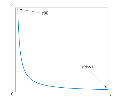
(i) Arabic numerals

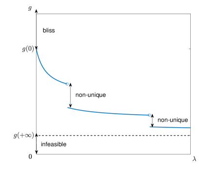
(ii) Case 1, discontinuous

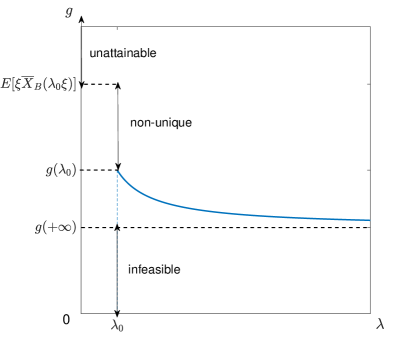
(iii) Case 2, continuous, $g(\lambda_{0})<+\infty=g(\lambda_{0}-)$

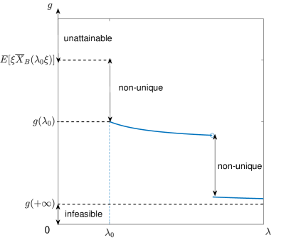
(iv) Case 2, discontinuous, $g(\lambda_{0})<+\infty=g(\lambda_{0}-)$

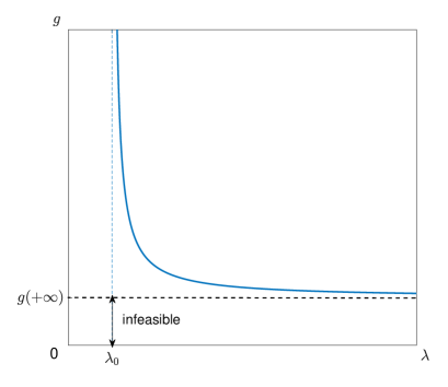
(v) Case 2, continuous, $g(\lambda_{0})=+\infty$

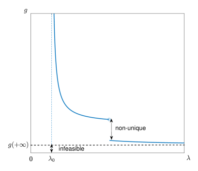
(vi) Case 2, discontinuous, $g(\lambda_{0})=+\infty$

Figure 1: Some examples for $g$. Case 3 is not included because $g$ is not finite. Especially, in Case 1, $g(0)$ can be finite or infinite and there is no bliss region for the latter. In Case 2, the term $\mathbb{E}[\xi\overline{X}_{B}(\lambda_{0}\xi)]$ can be finite or infinite, and there is no unattainable region for the latter. Meanwhile, in all three cases, the term $g(+\infty)$ may equal to or less than 0, and then there will be no infeasible region.

From Lemma 1 we know that $\underline{X}_{b}(\cdot)$ is nonincreasing and right-continuous on $[0,+\infty]$, while $\overline{X}_{b}(y)$ is nonincreasing and left-continuous. They both have countable discontinuous points. Moreover, $\underline{X}_{b}(\cdot)$ or $\overline{X}_{b}(\cdot)$ is discontinuous at $y\in(0,+\infty)$ if and only if its right limit does not equal to its left limit, i.e., $\underline{X}_{b}(y)\not=\overline{X}_{b}(y)$, which means that $\mathcal{X}_{b}(y)$ is not a singleton.

For $\lambda\in[0,+\infty]$, we take $X^{*}=\underline{X}_{B}(\lambda\xi)$ as a candidate of the measurable selection. Define

$$g(\lambda)=\mathbb{E}\left[\xi\underline{X}_{B}\left(\lambda\xi\right)\right].$$ (11)

As $\underline{X}_{B}(\lambda\xi)\geqslant\underline{x}_{B}$ and $\mathbb{E}[\xi\underline{x}_{B}]>-\infty$, we know

$$\mathbb{E}\left[\xi\underline{X}_{B}(\lambda\xi)^{-}\right]\leqslant\mathbb{E}[\xi\underline{x}_{B}^{-}]<+\infty.$$ (12)

Hence the expectation in (11) is well-defined, and $g(\lambda)>-\infty$ holds for any $\lambda\in[0,+\infty]$.

Different from the literature, there are two new features of $g$ in our discussion: finiteness and continuity. For the finiteness, there are three possible cases in terms of $g$ (Figure 1):

1. $g(\lambda)<+\infty$ for any $\lambda>0$.

2. There exists some $\lambda_{0}>0$ such that

   $$g(\lambda)<+\infty\text{ on }(\lambda_{0},+\infty),~{}g(\lambda)=+\infty\text{ on }(0,\lambda_{0}).$$ (13)

3. $g(\lambda)=+\infty$ for any $\lambda>0$.

Remark 2.

Proposition 1 is also a sufficient condition for Case 1 to hold; see the proof of Proposition 1 for details.

In the literature, Case 1 is always assumed to ensure the existence of the optimal Lagrange multiplier $\lambda^{*}$ (cf. Karatzas, Lehoczky and Shreve (1987); Kramkov and Schachermayer (1999)). From the perspective of Theorem 5, in the classical univariate problem (1), we can write $g(\lambda)=\mathbb{E}[\xi(u^{\prime})^{-1}(\lambda\xi)]$, which is a continuous function if $\xi$ is non-atomic. Therefore, for any $x_{0}$, one can adopt the intermediate value theorem and find a Lagrange multiplier $\lambda^{*}>0$ satisfying $g(\lambda)=x_{0}$ and solve the problem (cf. Jin, Xu and Zhou (2008)).

On the infiniteness issue of $g$, Case 2 and Case 3 are investigated in detail in this paper. In Theorem 3, we give a complete investigation of all three cases. For Case 3, Theorem 3(1) shows that either Problem (2) admits at most one feasible solution, or its optimal value equals $+\infty$. Case 2 is more complicated, as in this case, the optimal Lagrange multiplier may exist only for some $x_{0}$, though we are only using $\underline{X}_{B}(\lambda\xi)$ and $\overline{X}_{B}(\lambda\xi)$ as a representation of $\mathcal{X}_{B}(\lambda\xi)$, Theorem 3 shows that a finite optimal solution does not exist if we cannot find a finite optimal solution using $\underline{X}_{B}(\lambda\xi)$ and $\overline{X}_{B}(\lambda\xi)$.

On the continuity issue of $g$, $g$ may be discontinuous in our model. In fact, based on Lemma 1, we know that $\underline{X}_{b}(y)$ is nonincreasing and right-continuous with respect to $y$. The monotone convergence theorem implies that $g$ is nonincreasing and right-continuous, $g(\lambda_{0})=\lim\limits_{\lambda\to\lambda_{0}+}g(\lambda)$, which can be finite or infinite. However, $g$ is discontinuous at some $\lambda$ if the set of random variables $\mathcal{X}_{B}(\lambda\xi)$ is not a singleton, that is, $\underline{X}_{B}(\lambda\xi)<\overline{X}_{B}(\lambda\xi)$ happens with a positive probability value. In this case, to find an optimal solution for $x_{0}\in(g(\lambda),g(\lambda-))$, our basic technique is to “gradually” change $X^{*}$ from $\underline{X}_{B}(\lambda\xi)$ to $\overline{X}_{B}(\lambda\xi)$. As such, the value $\mathbb{E}[\xi X^{*}]$ will vary from $g(\lambda)$ to $g(\lambda-)$, and we will obtain an optimal solution. Significantly, we can construct infinitely many optimal solutions in this case. These results are concluded in Theorem 3.

Before we propose the main result of this section, we introduce the concept of the feasible set:

$$I\triangleq\left\{x_{0}:\text{Problem}~{}\eqref{problem1}~{}\text{has a feasible solution for the initial value}~{}x_{0}\right\}.$$

As we are considering $X$ and $x_{0}$ in the range of real numbers (that is, not necessarily positive), if $x_{0}<\mathbb{E}\left[\xi\underline{x}_{B}\right]$, the constraint $\mathbb{E}\left[\xi X\right]\leqslant x_{0}$ leads to $X<\underline{x}_{B}$ on a positive-measured set, and hence $\mathbb{E}\left[U(X,B)\right]=-\infty$. Moreover, as we are studying a state-dependent utility $U$, it may happens that $\mathbb{E}\left[U(X,B)\right]=-\infty$ even if $x_{0}\geqslant\mathbb{E}\left[\xi\underline{x}_{B}\right]$. Therefore, the notation $I$ is necessary. However, in most cases where $U$ is truncated from a CRRA utility, an S-shaped utility, or other utilities, $U$ has a lower bound itself in its domain. That is, if we have $X>\underline{x}_{B}$ almost surely, then we have $\mathbb{E}\left[U(X,B)\right]>-\infty$, and $I$ trivially becomes $\left[\mathbb{E}[\xi\underline{x}_{B}],+\infty\right]$ or $\left(\mathbb{E}[\xi\underline{x}_{B}],+\infty\right]$. To this light, we do not focus on whether the feasible set $I$ is trivial and use the following result to characterize the structure of the $I$.

Proposition 2.

Suppose that Assumption 1 holds. Exactly one of the following holds:

1. $I=[\mathbb{E}[\xi\underline{x}_{B}],+\infty)$;

2. $I=(\tilde{x},+\infty)$ for some $\tilde{x}\geqslant\mathbb{E}[\xi\underline{x}_{B}]$, where $\tilde{x}$ is allowed to equal $+\infty$.

Moreover, if $x_{0}=\mathbb{E}[\xi\underline{x}_{B}]$, there is at most one feasible solution and the candidate is $X=\underline{x}_{B}$. Finally, if $x_{0}\geqslant\mathbb{E}[\xi\overline{x}_{B}]$, Problem (2) admits a bliss solution.

In light of Proposition 2, the most complicated and unclear case of Problem (2) is $\mathbb{E}[\xi\underline{x}_{B}]<x_{0}<\mathbb{E}[\xi\overline{x}_{B}]$. In particular, when $\underline{x}_{B}\leqslant 0$ almost surely, every $x_{0}>0$ locates in this region as $\overline{x}_{B}$ is typically taken to be $+\infty$. When $\overline{x}_{B}<+\infty$ and $\mathbb{E}[\xi\overline{x}_{B}]<+\infty$, it means that $U(\cdot,B)$ is a constant on $[\overline{x}_{B},+\infty)$, and it is possible to obtain a bliss solution for large $x_{0}$. Proposition 2 shows that $I$ is a connected interval with the right endpoint being $+\infty$, but we do not know its left endpoint, which depends highly on $U$ and $B$. In the rest of the paper, we will focus mainly on the case that $\mathbb{E}[\xi\underline{x}_{B}]<x_{0}<\mathbb{E}[\xi\overline{x}_{B}]$ with $x_{0}\in I$.

Remark 3.

Practically, $\underline{x}_{B}>-\infty$ means that the manager cannot bear a loss exceeding $-\underline{x}_{B}$, and then the condition $x_{0}\geqslant\mathbb{E}\big{[}\xi\underline{x}_{B}\big{]}$ requires enough initial capital to face the potential risk. Moreover, if $x_{0}$ is large enough such that $\mathbb{E}[\xi\overline{x}_{B}]<x_{0}<+\infty$, then the manager can reach the maximal utility without any risk. Hence the results indicate that people with a high tolerance for loss are easy to find a satisfactory strategy, while people who are easy to be satisfactory or have enough initial capital will obtain a bliss solution.

Based on the notation $I$, we introduce our results on optimal solutions in all of the Cases 1-3. Noting that $g(\lambda_{0})=\lim\limits_{\lambda\to\lambda_{0}+}g(\lambda)$, which may be finite or infinite. In the following context, $\mathbb{E}\left[\xi\overline{X}_{B}(\lambda_{0}\xi)\right]$ is also allowed to be $+\infty$.

Theorem 3.

Suppose that $(\Omega,\mathcal{F},\mathbb{P})$ is non-atomic and Assumptions 1-2 hold.

1. If Case 3 holds, then Problem (2) is infinite for any $x_{0}\in I\backslash\{\mathbb{E}[\xi\underline{x}_{B}]\}$.

2. If Case 1 or Case 2 holds, then we have $\lambda_{0}\in[0,+\infty)$ in (13). Suppose that $x_{0}\in I$. We have:

   1. if there exists a real number $\lambda^{*}\geqslant\lambda_{0}$ such that $g(\lambda^{*})=x_{0}$, then $X^{*}=\underline{X}_{B}\big{(}\lambda^{*}\xi\big{)}$ is an optimal solution;

   2. if $g(\lambda^{*})<x_{0}\leqslant g(\lambda^{*}-)$ for some discontinuous point $\lambda^{*}>\lambda_{0}$, it has a positive probability that the set $\mathcal{X}_{B}\big{(}\lambda^{*}\xi\big{)}$ is not a singleton. Moreover, if $x_{0}=g(\lambda^{*}-)$, then $X^{*}=\overline{X}_{B}(\lambda^{*}\xi)$ is an optimal solution; if $x_{0}<g(\lambda^{*}-)$, there are infinitely many optimal solutions;

   3. (for Case 1, where $\lambda_{0}=0$) if $x_{0}\geqslant g(\lambda_{0})=g(0)$, then we have a bliss solution;

   4. (for Case 2, where $\lambda_{0}\!\!>\!0$) let $\theta=\mathbb{E}[\xi\overline{X}_{B}(\lambda_{0}\xi)]$. If $x_{0}=\theta$, then $\overline{X}_{B}(\lambda_{0}\xi)$ is an optimal solution; if $g(\lambda_{0})<x_{0}<\theta$, there are infinitely many optimal solutions. if $x_{0}>\theta$, Problem (2) has no finite optimal solutions. We have a sequence $\{\hat{X}_{k}\}_{k\geqslant 1}$ converging almost surely to $\underline{X}_{B}(\lambda_{0}\xi)$ with $\mathbb{E}\left[\xi\hat{X}_{k}\right]=x_{0}$ and

      $$\sup_{X:\mathbb{E}\left[\xi X\right]\leqslant x_{0}\atop U(X,B)>-\infty}\mathbb{E}\left[U(X,B)\right]=\lim_{k\to+\infty}\mathbb{E}\left[U\left(\hat{X}_{k},B\right)\right]{\color[rgb]{0,0,0}=}\mathbb{E}\left[U\left(\overline{X}_{B}\left(\lambda_{0}\xi\right),B\right)\right]+\lambda_{0}(x_{0}-\theta).$$ (14)

Remark 4.

We point out that in Theorem 3(2)(a), (b) when $x_{0}=g(\lambda^{*})$ and (c2) when $x_{0}=\mathbb{E}[\xi\overline{X}_{B}(\lambda_{0}\xi)]$, the optimal solution is unique if we further require Assumption 3. This is also proved in Appendix B.3.

Theorem 3 gives tractable methods to find out optimal solutions of Problem (2) using $g$ and answers the question that Theorem 2 leaves. Specifically, Theorem 2 shows that a necessary and sufficient condition for $X$ to be an optimal solution is that $X\in\mathcal{X}_{B}(\lambda\xi)$ for some $\lambda$ satisfying $\mathbb{E}[\xi X]=x_{0}$. Here we need an extra work of measurable selection on $\mathcal{X}_{B}(\lambda\xi)$, and Theorem 3 proves the existence of such a selection by construction. (a) and (b) deal with the case $x_{0}\in\left(g(+\infty),g(\lambda_{0})\right]$, while (c1) and (c2) aim at the situation $x_{0}>g(\lambda_{0})$. For the rest case $x_{0}\leqslant g(+\infty)=\mathbb{E}[\xi\underline{x}_{B}]$, we have discussed the case in Proposition 2.

The parts (c1) and (c2) of Theorem 3 (when $x_{0}>g(\lambda_{0})$) are first investigated in this paper. Most literature only concentrates on Case 1. In our models, when a benchmark $B$ is involved, the issue of measurable selection arises. Here, our $g$ considers $\underline{X}_{B}$ as a candidate. We have shown the existence of a measurable selection satisfying the budget constraint. Based on Theorem 3 and Proposition 2, we figure out the (non-)existence and (non-)uniqueness of an optimal solution for all scenarios.

The result of non-unique solutions is because of the generality of both $U$ and $B$. On the one hand, if $U$ is strictly concave, then $\mathcal{X}_{b}(y)$ contains always one element, and non-unique optimal solutions described in (b) will not occur. On the other hand, if $B$ is deterministic, then $\mathcal{X}_{B}(\lambda\xi)$ is not a singleton if and only if $\lambda\xi$ lies in the discontinuous point set of $\overline{X}_{B}$. Noting that $\overline{X}_{B}$ is decreasing, the set is countable. As such, the probability that the random set $\mathcal{X}_{B}\big{(}\lambda^{*}\xi\big{)}$ is not a singleton equals zero when the pricing kernel $\xi$ is non-atomic, which means that the non-unique optimal solutions will not happen either. Therefore, it is only a special case of Problem (2).

Table 1: Solutions of Problem (2) when Assumptions 1-3 hold and $\inf I=\mathbb{E}[\xi\underline{x}_{B}]$. Note: Denote by $\lambda^{*}\in(\lambda_{0},+\infty)$ a discontinuous point of $g$.

	Case 1	Case 2	Case 3
$x_{0}<\mathbb{E}[\xi\underline{x}_{B}]=g(+\infty)$	infeasible (Proposition 2)
$x_{0}=\mathbb{E}[\xi\underline{x}_{B}]=g(+\infty)$	at most one feasible solution $\underline{x}_{B}$ (Proposition 2)
$x_{0}\in g([\lambda_{0},+\infty))$	unique (Thm 3(2)(a))		infinite (Thm 3(1))
$x_{0}\in(g(\lambda^{*}),g(\lambda^{*}-))$	non-unique (Thm 3(2)(b))
$x_{0}=g(\lambda^{*}-)$	unique (Thm 3(2)(b))
$x_{0}>g(\lambda_{0})$	bliss (Thm 3(2)(c1))	$x_{0}>\mathbb{E}[\xi\overline{X}_{B}(\lambda_{0}\xi)]$: unattainable (Thm 3(2)(c2))
		$x_{0}=\mathbb{E}[\xi\overline{X}_{B}(\lambda_{0}\xi)]$: unique (Thm 3(2)(c2))
		$x_{0}<\mathbb{E}[\xi\overline{X}_{B}(\lambda_{0}\xi)]$: non-unique (Thm 3(2)(c2))

Remark 5.

As $B$ can be any random variable, the optimal solution $\underline{X}_{B}(\lambda^{*}\xi)$ may not be a function of $\xi$. Moreover, as the function $\underline{X}_{b}(y)$ performs no obvious monotonicity in $b$, $\underline{X}_{B}(\lambda^{*}\xi)$ may not be a decreasing function of $\xi$ even if $B$ is a function of $\xi$, and it may not be comonotonic with $\xi$; see Bernard, Moraux, Rüschendorf and Vanduffel (2015) for a concrete model. This phenomenon also appears in the literature using quantile formulation. In Jin and Zhou (2008), He and Zhou (2011), and Xu (2016), the optimal solution is a decreasing function of the pricing kernel, while in Peng, Wei and Xu (2023) where a CPT reference and a stochastic benchmark are adopted, the optimal solution may not be a decreasing function of the pricing kernel (though it is still comonotonic with the pricing kernel).

For the finiteness and attainability, as our results in Theorem 3 (2)(a)(b)(c1) (and (c2) when $x_{0}\leqslant\theta$) are tractable, Problem (2) is attainable in all these situations, and one can verify the finiteness directly. For the remaining case (c2) with $x_{0}>\theta$, Theorem 3 indicates that $\theta$ is the largest initial value for which we can find an optimal solution through $g$ (noting that $\theta$ can be $+\infty$). For this initial value $x_{0}$, we have an optimal solution $\overline{X}_{B}(\lambda_{0}\xi)$, and we can verify the finiteness of Problem (2). We have two cases:

• If Problem (2) is finite for $\theta$, then (14) shows that for the initial value $x_{0}$, Problem (2) is also finite. Moreover, Theorem 3 asserts that there is no optimal solution, i.e., the problem is unattainable for $x_{0}$.

• If Problem (2) is infinite for $\theta$, then as $x_{0}>\theta$ and $U(x,b)$ is nondecreasing in $x$, we can simply turn up the infinite optimal solution $\overline{X}_{B}(\lambda_{0}\xi)$ for Problem (2) with initial value $\theta$ to obtain an infinite optimal solution with initial value $x_{0}$.

In a word, we can use the function $g$ and Theorem 3 to completely figure out the existence and expressions of optimal solutions, finiteness and attainability of Problem (2), while Theorem 2 gives support on the uniqueness of the optimal solution.

To end this section, we propose an example where there may be infinitely many optimal solutions. We provide more detailed characterizations of these solutions and select a specific optimal solution by investigating the liquidation probability.

Example 3 (Infinitely many solutions and further selection).

Let $\{W_{t}\}_{0\leqslant t\leqslant T}$ be a standard Brownian motion. Let $S_{t}=\exp\left\{\left(\mu-\frac{1}{2}\sigma^{2}\right)t+\sigma W_{t}\right\}$ be the risky asset and $F_{t}=e^{rt}$ be the risk-free asset with $\mu>r>0$ and $\sigma>0$. Then $\xi=\exp\left[-\left(r+\frac{1}{2}\theta^{2}\right)T-\theta W_{T}\right]$ follows a log-normal distribution with $\theta=\frac{\mu-r}{\sigma^{2}}$. For the benchmark $B$, we follow Basak, Pavlova and Shapiro (2007) to set a general value-weighted benchmark portfolio process:

$$\left\{\begin{aligned} &\mathrm{d}B_{t}=\alpha rB_{t}\mathrm{d}t+\beta B_{t}\left(\frac{\mathrm{d}S_{t}}{S_{t}}\right),\\ &B_{0}=bx_{0},\end{aligned}\right.$$ (15)

and $B=B_{T}$, where $\alpha+\beta=1,~{}b\geqslant 0$ are fixed constant parameters. Define the utility as

$$U(x,b)=\left\{\begin{aligned} &(x-b)^{p},&&x>b,\\ &-k(b-x)^{p},&&0\leqslant x\leqslant b.\\ \end{aligned}\right.$$ (16)

where $k>1,p\in(0,1)$ are constants. Under this setting, we have

$$B=bx_{0}e^{\left(\alpha r+\beta\mu-\frac{\beta^{2}\sigma^{2}}{2}\right)T+\beta\sigma W_{T}}=L\xi^{-\frac{\beta\sigma}{\theta}},$$

where $L$ is a constant depending on the market parameters. For the S-shaped utility, we have

$$\mathcal{X}_{b}(y) =\left\{\begin{aligned} &\{0\},&&b-dI(y)>0,\\ &\{0,b+I(y)\},&&b-dI(y)=0,\\ &\{b+I(y)\},&&b-dI(y)<0,\\ \end{aligned}\right.$$

where $I(y)=\left(\frac{y}{p}\right)^{\frac{1}{p-1}}$ and $d>0$ is the unique solution of the tangent equation $1+kd^{p}=p(d+1)$. Therefore, $\mathcal{X}_{B}(\lambda\xi)$ has more than one element if and only if $B=dI(\lambda\xi)$, that is,

$$L\xi^{-\frac{\beta\sigma}{\theta}}=d\left(\frac{\lambda\xi}{p}\right)^{\frac{1}{p-1}}.$$

When $\frac{\beta\sigma}{\theta}=\frac{1}{1-p}$ and $\lambda_{0}=p\left(\frac{L}{d}\right)^{p-1}$, we have $B=dI(\lambda_{0}\xi)$ holds almost everywhere, and $\mathcal{X}_{B}(\lambda_{0}\xi)=\{0,\frac{d+1}{d}B\}$ is a binary set. Using Theorem 3, this $\lambda_{0}$ is a discontinuous point of $g$, and we have $g(\lambda_{0}+)=0$, $g(\lambda_{0}-)=\frac{d+1}{d}\mathbb{E}\left[\xi B\right]=\frac{d+1}{d}L\mathbb{E}\left[\xi^{\frac{p}{p-1}}\right]\triangleq C$. For $0<x_{0}<C$, we have infinitely many optimal solutions. Indeed, for every $A\in\mathcal{F}$, define $X^{A}=\frac{d+1}{d}B\mathds{1}_{A}\in\mathcal{X}_{B}(\lambda_{0}\xi)$, if $\mathbb{E}\left[\xi X^{A}\right]=\frac{d+1}{d}L\mathbb{E}\left[\xi^{\frac{p}{p-1}}\mathds{1}_{A}\right]=x_{0}$, then Theorem 2 indicates that $X^{A}$ is an optimal solution.

Among all these solutions, we can find one with the smallest liquidation probability $\mathbb{P}\left[X^{A}=0\right]$ (=$P(A)$). If we fix $P(A)=\varepsilon>0$, then $\mathbb{E}\left[\xi^{\frac{p}{p-1}}\mathds{1}_{A}\right]$ attains its minimum when $A$ has the form $A=\{\omega:W_{T}<\sqrt{T}\Phi^{-1}(\varepsilon)\}$, where $\Phi$ is the cumulative distribution function of the standard normal distribution. This is because $\xi$ is decreasing with $W_{T}$. The minimum value is $m(\varepsilon)=\frac{d+1}{d}Le^{\frac{p}{1-p}(r+\frac{\theta^{2}}{2(1-p)})T}\Phi\left(\Phi^{-1}(\varepsilon)-\frac{p\theta}{1-p}\sqrt{T}\right).$ Similarly, we can prove that the maximum value of $\mathbb{E}\left[\xi^{\frac{p}{p-1}}\mathds{1}_{A}\right]$ is $M(\varepsilon)=\frac{d+1}{d}Le^{\frac{p}{1-p}(r+\frac{\theta^{2}}{2(1-p)})T}\Phi\left(\Phi^{-1}(\varepsilon)+\frac{p\theta}{1-p}\sqrt{T}\right).$ Letting $m(\varepsilon)\leqslant x_{0}\leqslant M(\varepsilon)$, we can solve the range of the liquidation probability $\varepsilon$ from $x_{0}$. Moreover, we conclude that when $X^{A}$ attains the minimal liquidation probability $\varepsilon_{m}$, its liquidation happens only for large $W_{T}>\sqrt{T}\Phi^{-1}(\varepsilon_{m})$, which means that the market is bad. While $X^{A}$ attains the maximal liquidation probability $\varepsilon_{M}$, its liquidation happens only for small $W_{T}<\sqrt{T}\Phi^{-1}(\varepsilon_{M})$, which means that the market is good.

5 Well-definedness and finiteness

In this section, we give some further results on the well-definedness and finiteness (we have already given a sufficient condition in Proposition 1). Based on (26)-(28) in the proof of Proposition 1, we can also verify the finiteness of Problem (2) using $g$ and $\underline{X}_{B}$. We have:

Proposition 3.

Suppose that Assumption 1 holds. If there exists $\lambda\in[0,+\infty)$ such that $g(\lambda)$ is finite, and $\mathbb{E}\left[U\left(\underline{X}_{B}(\lambda\xi),B\right)\right]$ is well-defined and finite, then Problem (2) is well-defined and finite for all $x_{0}\in\mathbb{R}$.

In light of Proposition 3, we can also study the finiteness of Problem (2) using $g$ and

$$J(\lambda)\triangleq\mathbb{E}\left[U\left(\underline{X}_{B}(\lambda\xi),B\right)\right],~{}\lambda\in(0,+\infty).$$ (17)

Assumption 4 (Well-definedness of $J$).

The expectation in (17) is well-defined for any $\lambda\in(0,+\infty)$ and $J(\lambda)>-\infty$ for all $\lambda\in(0,+\infty)$.

Under Assumption 4, similarly as $\lambda_{0}$ in (13), we define $\lambda_{1}\in[0,+\infty]$ from

$$J(\lambda)<+\infty\text{ for }\lambda\in(\lambda_{1},+\infty),~{}J(\lambda)=+\infty\text{ for }\lambda\in(0,\lambda_{1}).$$

We have the following results on the value function of Problem (2):

Theorem 4.

Suppose that Assumptions 1-2 and 4 hold and $x_{0}\in I\backslash\{\mathbb{E}[\xi\underline{x}_{B}]\}$, then

1. If $\lambda_{0}=+\infty$, then Problem (2) is infinite;

2. If $\lambda_{0}<+\infty$, but $\lambda_{1}=+\infty$, then Problem (2) is infinite;

3. If $\lambda_{0}<+\infty$, and $\lambda_{1}<+\infty$, then Problem (2) is finite, and we have $\lambda_{1}=\lambda_{0}$.

Remark 6.

Theorem 4 indicates that under Assumption 4, if Problem (2) is finite (or infinite) for one $x_{0}$ in the feasible set, then it is finite (or infinite) for all $x_{0}$ in the feasible set. In this light, we can first compute $g$ and $J$ to verify the finiteness of Problem (2), and then we use Theorem 3 to find a finite solution or an infinite solution.

6 Connection to the univariate framework

In this section, we connect our results to the univariate framework of general utilities, while we assume that $u$ satisfies good conditions (differentiable and strictly concave) in Problem (1). The univariate utility is state-independent and the univariate framework depends only on the distribution of the wealth $X$, and hence the objective is distribution-invariant. Fix $u$ satisfying Assumption 1 (we can regard $u$ as a state-dependent utility $U(x,b)$ with constant state). For $y\geqslant 0$, define the conjugate set function $\mathcal{X}$ as

$$\mathcal{X}(y)=\mathop{\arg\sup}\limits_{x\in\mathbb{R}\cup\{\pm\infty\}}{\left[u(x)-yx\right]}.$$

Define $\underline{X}(y)=\inf\mathcal{X}(y),~{}\overline{X}(y)=\sup\mathcal{X}(y)$ as well as $g(\lambda)=\mathbb{E}\left[\xi\underline{X}(\lambda\xi)\right]$, and $\lambda_{0}$ as in (13).

Here the slope of $u$ near $+\infty$ can be positive. For simplicity, we assume that $\xi$ is integrable, then one can verify that the feasible set $I=\left[\underline{x}\mathbb{E}\left[\xi\right],+\infty\right)$ or $\left(\underline{x}\mathbb{E}\left[\xi\right],+\infty\right)$, which depends on the type of $\underline{x}$. Moreover, Assumption 2 is also easy to verify.

Using the results in Sections 3-5, we propose a complete result for the univariate utility $u$ in Theorem 5 and the following discussion.

Theorem 5.

Suppose that $(\Omega,\mathcal{F},\mathbb{P})$ is non-atomic and that the univariate version of Assumptions 1 and 3 hold.

(1) $X^{*}$ is an optimal solution of Problem (1) if and only if there exists $\lambda^{*}\geqslant 0$ such that $X^{*}\in\mathcal{X}(\lambda^{*}\xi)$ and $\mathbb{E}\left[\xi X^{*}\right]=x_{0}$.

(2) The optimal solution is unique if the set $\mathcal{X}(y)$ is singleton for any $y\geqslant 0$ or $\xi$ is non-atomic. The set of optimal solutions $\mathcal{X}(\lambda^{*}\xi)$ may be non-unique if $u$ is non-concave and $\xi$ is atomic.

Theorem 5 is a complete result for general (discontinuous and non-concave) utilities, which extends the univariate results in literature; see Jin, Xu and Zhou (2008) and Reichlin (2013). Under our framework, Theorem 5 becomes a direct corollary of the multivariate version Theorems 1-2: to prove Theorem 5, one can simply regard $B$ as a constant in Theorems 1-2 (removing all the $``B"$ appeared in the proof). Thus, our framework also serves to offer proof for the univariate result. Apart from the uniqueness, for $x_{0}\in\mathbb{R}$ we also have:

1. When $\lambda_{0}=+\infty$, the problem is infinite for every $x_{0}\in\left(\underline{x}\mathbb{E}\left[\xi\right],+\infty\right)$. For $x_{0}<\underline{x}\mathbb{E}\left[\xi\right]$, there is no feasible solutions. While for $x_{0}=\underline{x}\mathbb{E}\left[\xi\right]$, there is at most one feasible solution, which depends on the type of $\underline{x}$.

2. When $\lambda_{0}\in(0,+\infty)$, the optimal solution(s) exists for all $x_{0}\in\left(\underline{x}\mathbb{E}\left[\xi\right],\mathbb{E}\left[\xi\overline{X}(\lambda_{0}\xi)\right]\right]$, and one can directly verify the finiteness or infiniteness of the solution. For $x_{0}>\mathbb{E}\left[\xi\overline{X}(\lambda_{0}\xi)\right]\triangleq\theta$, we have two cases:

   • If the problem with initial value $\theta$ is finite, the problem for $x_{0}$ is finite and unattainable, and we can find a sequence $\{\hat{X}_{k}\}$ converges to $\overline{X}(\lambda_{0}\xi)$ almost surely satisfying $\mathbb{E}\left[\xi\hat{X}_{k}\right]=x_{0}$, $u(\hat{X}_{k})>-\infty$ and

     $$\sup\limits_{X:\mathbb{E}[\xi X]\leqslant x_{0}\atop u(X)>-\infty}\mathbb{E}[u(X)]=\lim_{k\to+\infty}\mathbb{E}\left[u(\hat{X}_{k})\right]=\mathbb{E}\left[u\left(\overline{X}(\lambda_{0}\xi)\right)\right]+\lambda_{0}(x_{0}-\theta).$$ (18)

   • If the problem with initial value $\theta$ is infinite, then it is also infinite with initial value $x_{0}$, and an optimal solution $X^{*}$ can be obtained by letting the optimal solution $\overline{X}(\lambda_{0}\xi)$ for initial value $\theta$ satisfy $\mathbb{E}\left[\xi X^{*}\right]=x_{0}$.

3. When $\lambda_{0}=0$, then for each $x_{0}>\underline{x}\mathbb{E}\left[\xi\right]$ there exists an optimal solution, and the finiteness or infiniteness can be verified directly.

In Reichlin (2013), it is claimed that there exists $\tilde{x}\in(0,+\infty]$ such that for $x_{0}\in(0,\tilde{x})$, Problem (1) admits an optimal solution. While in Theorem 5, $\tilde{x}$ can be indeed determined as $\tilde{x}=\mathbb{E}\left[\xi\overline{X}(\lambda_{0}\xi)\right]$, and the case when $x_{0}\geqslant\tilde{x}$ is also supplemented. The result of a differentiable and strictly concave function $u$ exists in Jin, Xu and Zhou (2008) and Karatzas and Shreve (1998); in this case, we have $\mathcal{X}=(u^{\prime})^{-1}$ and $X^{*}=(u^{\prime})^{-1}(\lambda^{*}\xi)$.

A key insight of Theorem 5 is that there may also exist non-unique solutions in the univariate framework. It may only happen if $u$ is non-concave and $\xi$ is atomic. In this case, the random set $\mathcal{X}(\lambda^{*}\xi)$ is not a singleton and $g(\lambda):=\mathbb{E}[\xi\mathcal{X}(\lambda\xi)]$ is discontinuous at the Lagrange multiplier $\lambda^{*}$. The optimal solution is unique if $\xi$ is non-atomic. However, in the multivariate framework, even if $\xi$ is non-atomic, there may exist non-unique solutions. It is because of the state-dependent utility $U$ and the stochastic benchmark $B$. They lead to a non-singleton random set $\mathcal{X}(\lambda^{*}\xi)$.

Traditionally, the optimal solution for the affine utility is known to be $X^{*}=+\infty$ if the pricing kernel $\xi$ is non-atomic. We finally propose Example 4, showing that for the affine utility, $\xi$ must be atomic for the optimal solution to exist. We claim that the affine utility, although not satisfying Assumption 1, satisfies Assumption 5 in the Appendix B, where we show that Theorems 2-3 also hold under the weaker but more complex Assumption 5.

Example 4 (Affine utility).

Fix $k\in(0,+\infty)$ and $L\in\mathbb{R}$. Let $u(x)=kx,~{}x\geqslant L.$ For any $x_{0}>L\mathbb{E}[\xi]$, we find that the optimal solution exists if and only if $\xi_{min}\triangleq\mathrm{ess\mbox{-}inf}\xi\in(0,+\infty)$ and $\xi$ has an atom at $\xi_{min}$. Indeed, if the optimal solution exists, it is given by $X^{*}\in\mathcal{X}(\lambda^{*}\xi)$, where $\lambda^{*}\in(0,+\infty)$ is a constant (to be determined) and

$$\mathcal{X}(y)=\left\{\begin{aligned} &L,&&y>k;\\ &[L,+\infty],&&y=k;\\ &+\infty,&&0\leqslant y<k.\end{aligned}\right.$$

To satisfy $\mathbb{E}[\xi X^{*}]=x_{0}$, we obtain that $\lambda^{*}=k/\xi_{min}$ and the optimal solution is

$$X^{*}=\left\{\begin{aligned} &L,&&\xi>\xi_{min};\\ &\frac{x_{0}-L\mathbb{E}\left[\xi\mathds{1}_{\{\xi>\xi_{min}\}}\right]}{\xi_{min}\mathbb{P}[\xi=\xi_{min}]},&&\xi=\xi_{min}.\end{aligned}\right.$$

This result indicates that the optimal terminal wealth $X^{*}$ will gamble on the atomic $\xi=\xi_{min}$ and keep the lowest level $L$ for other cases.

7 Application

In this section, we formulate a constrained utility optimization problem with state-dependent benchmarks:

$$\begin{split}&\sup_{X\geqslant 0}\mathbb{E}\left[U\left(X,B_{1}\right)\right]\\ &\text{subject to}~{}\mathbb{E}[\xi X]\leqslant x_{0},~{}\mathbb{P}[X\geqslant B_{2}]\geqslant 1-\alpha,\\ \end{split}$$ (19)

where $U$ is the S-shaped utility function defined in Example 2, $B_{1}$ is a performance benchmark (reference level) and $B_{2}$ is a risk benchmark. $\xi$ is a log-normal pricing kernel with the form $\xi=\exp(-(r+\frac{1}{2}\theta^{2})T-\theta\sqrt{T}W),$ where $r$ is the risk-free rate of interest, $\theta$ is the risk premium, and $W$ follows a standard normal distribution.

In the literature of risk management with VaR constraints (cf. Nguyen and Stadje (2020)), $B_{2}$ is usually taken as a constant $L$, which means the worst level of return under the given confidence level. However, when the market state is not bad, it is reasonable to require a higher level of return. If we raise $L$ only in the situation when the market does not perform poorly, the risk of the return will not become larger. That is, we allow $B_{2}$ (and also $B_{1}$) to be stochastic.

In the next subsection, we propose a general solution to Problem (19). In consideration of the numerical results, we will only consider three simple plans as follows (where $L_{i}$ and $w$ are constants):

Plan I: $B_{1}=L_{1}$, $B_{2}=L_{3}$.

Plan II: $B_{1}=L_{1}$, $B_{2}=L_{3}+(L_{4}-L_{3})\mathds{1}_{\{W>w\}}$. Note that $B_{2}$ is state-dependent.

Plan III: $B_{1}=L_{1}+(L_{2}-L_{1})\mathds{1}_{\{W>w\}}$, $B_{2}=L_{3}+(L_{4}-L_{3})\mathds{1}_{\{W>w\}}$. Note that both $B_{1}$ and $B_{2}$ are state-dependent.

Plan I is the most classical case. In Plan II, we adjust the level of return in the VaR constraint from $L_{3}$ to $L_{4}$ when the market is not bad, while in Plan III, the performance benchmark $B_{1}$ will also be raised from $L_{1}$ to $L_{2}$. For simplicity, we also assume $B_{1}>B_{2}$. To solve Problem (19), we apply the Lagrange method to convert it to Problem (2). In literature, the quantile formulation method is adopted to solve an optimization problem with risk management, but the validity of this method requires the objective function to be distribution-invariant, i.e., the values of the objective function are the same for identically distributed random variables $X$. As the objective function involves stochastic benchmarks $B_{1}$ and $B_{2}$ in Problem (19), the quantile formulation method does not work here.

7.1 Theoretical results: state-dependent utility optimization

For $\mu\geqslant 0$, define the modified utility function

$$U^{\mu}(x,(b_{1},b_{2}))=\left\{\begin{array}[]{ll}U(x,b_{1})+\mu\mathds{1}_{\{x\geqslant b_{2}\}},&x\geqslant 0,\\ -\infty,&x<0.\end{array}\right.$$

Denote $b=(b_{1},b_{2})$ and $B=(B_{1},B_{2})$. Consider the converted problem without the risk constraint:

$$\begin{split}&\sup_{X\geqslant 0}\mathbb{E}\left[U^{\mu}\left(X,B\right)\right]\\ &\text{subject to}~{}\mathbb{E}[\xi X]\leqslant x_{0}.\\ \end{split}$$ (20)

Under Plans I-III, we have the following result.

Theorem 6.

For every $x_{0}>0$, Problem (20) admits a unique finite optimal solution $X^{\mu}=\underline{X}^{\mu}_{B}(\lambda(\mu)\xi)$ with $\lambda(\mu)$ as a function of $\mu$. When $b_{1}>b_{2}$, the function $\underline{X}_{b}^{\mu}(y)$ is given as follows:

$$①.~{}~{}~{}~{}\text{if}~{}y_{1}(b)\leqslant y_{2}^{\mu}(b),~{}\text{then} ②.~{}~{}~{}~{}\text{if}~{}y_{1}(b)\geqslant y_{2}^{\mu}(b),~{}\text{then}$$

$$\underline{X}_{b}^{\mu}(y)=\left\{\begin{array}[]{ll}b_{1}+\left(\frac{p}{y}\right)^{\frac{1}{1-p}},&y<y_{1}(b),\\ b_{2},&y_{1}\leqslant y<y_{2}^{\mu}(b),\\ 0,&y\geqslant y_{2}^{\mu}(b),\end{array}\right. \underline{X}_{b}^{\mu}(y)=\left\{\begin{array}[]{ll}b_{1}+\left(\frac{p}{y}\right)^{\frac{1}{1-p}},&y<y_{3}^{\mu}(b),\\ 0,&y\geqslant y_{3}^{\mu}(b),\end{array}\right.$$

where $y_{1}(b)$, $y_{2}^{\mu}(b)$ and $~{}y_{3}^{\mu}(b)$ are defined by

$$\footnotesize y_{1}(b)=p\left(\frac{d(k)}{b_{1}-b_{2}}\right)^{1-p},~{}y_{2}^{\mu}(b)=\frac{1}{b_{2}}\left(\mu+kb_{1}^{p}-k(b_{1}-b_{2})^{p}\right),~{}y_{3}^{\mu}(b)=p\left(\frac{d(k+\mu b_{1}^{-p})}{b_{1}}\right)^{1-p},$$

and $d(s)$ denotes the solution of the equation $1+sx^{p}=p(x+1)$.

Based on Theorem 6, we solve the equation $\mathbb{P}[X^{\mu}\geqslant B_{2}]=1-\alpha$ to determine the Lagrange multiplier $\mu^{*}$, and then $X^{*}:=X^{\mu^{*}}$ gives a finite optimal solution of Problem (19).

Remark 7.

The existence of $\mu^{*}$ is not a trivial issue, and for some initial value $x_{0}$ there may be no such $\mu^{*}$. But this is not the key point of this paper; see e.g. Wei (2018) for details.

7.2 Numerical results

The following figure shows the numerical result of the relation between $X^{*}$ and $\xi$ in Plans I, II and III respectively. The parameter is taken as $r=0.03$, $\theta=0.3$, $T=10$, $p=0.5$, $k=2.25$, $x_{0}=30$, $L_{1}=60$, $L_{2}=70$, $L_{3}=40$, $L_{4}=50$, $w=-1$, $\alpha=0.05$. The top axis shows the cumulative probability of $\xi$ from left to right.

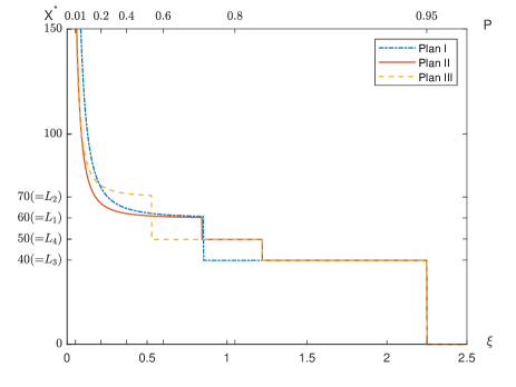
Figure 2: relationship between $X^{*}$ and $\xi$.

We know from Figure 2 that, if we adjust the return level higher in the VaR when the market is not bad, that is, we change from Plan I to Plan II, then the return performs better when $\xi\in[0.85,1.22]$ with a stable increment from $L_{3}(=40)$ to $L_{4}(=50)$, and the probability is about 10.8%. While for $\xi<0.85$, the return of Plan I is higher than that of Plan II. That is, when the market performs well, Plan I gives a higher return than Plan II, and the gap will increase rapidly from $0$ as $\xi$ decreases. Moreover, for a small probability ($<1$%, when the market performs quite well), the relative gap between Plan I and Plan II reaches more than $50\%$. In conclusion, compared to Plan I, Plan II (different $B_{2}$) increases the return when the market is not too bad by reducing the return when the market is quite good, which suits bearish managers or people with a high risk aversion.

In Plan III, the manager has higher anticipation than in Plan II when the market does not perform poorly. The result shows that his return becomes higher than Plan II when $\xi<0.53$ with a probability of about $54.8\%$, and the gap decays quickly to $0$ when $\xi$ decreases (which means that the market state is better). While for $\xi\in[0.53,0.84]$, Plan II gives a higher return than Plan III, and the probability is about 18.3%. Therefore, compared to Plan II, Plan III (different $B_{1}$) increases the return when the market is relatively good by reducing the return when the market is relatively bad, which suits bullish managers or people with a low risk aversion. As Plan I cares least about the risk among the three plans, its return for $\xi<0.2$ (when the market performs quite well) is the highest, and the probability is about 18.42%.

Remark 8.

In Plans II and III, we have $\mathbb{P}[X^{*}\geqslant L_{3}]=0.95$, which is the first stage of the risk value $B_{2}$. For the second stage, we have $\mathbb{P}[X^{*}\geqslant L_{4}]=0.84$, and events of reaching the second stage are equivalent to the event that $\xi<1.22$. As a possible extension, we consider a risk variable with multiple stages such as:

$$B_{2}=f(\xi)=L_{1}\mathds{1}_{(\xi_{1},+\infty)}(\xi)+\sum_{k=2}^{n-1}L_{k}\mathds{1}_{(\xi_{k},\xi_{k-1}]}(\xi)+L_{n}\mathds{1}_{(-\infty,\xi_{n}]}(\xi),$$

which may become an alternative for the model with multiple risk constraints as

$$\mathbb{P}[X\geqslant L_{i}]\geqslant 1-\alpha_{i},~{}i=1,2,...,n.$$

Remark 9.

Apart from Plans I-III, if we take $B_{1}-B_{2}=d(k)\big{(}\frac{\xi}{p}\big{)}^{\frac{1}{p-1}}$, then $y_{1}(B)=\xi$, and $g(\lambda)$ may be discontinuous at $\lambda=1$. In this case, Theorem 3 shows that there may exist infinitely many optimal solutions.

8 Concluding remarks

We propose a framework of state-dependent utility optimization with general benchmarks. We give a detailed and complete discussion on the feasibility, finiteness, and attainability. We find that: (i) the optimal solutions may be a random set, which possibly consists of infinitely many optimal solutions; (ii) the Lagrange multiplier may not exist because the function $g$ in (11) is discontinuous or infinite at some $\lambda^{*}$; (iii) the measurability issue may arise when applying the concavification to a multivariate utility function and when selecting a candidate from the non-unique optimal solutions. We address these technical issues, especially for measurability, and we do not assume a priori that the optimal Lagrange multiplier exists. In light of (i) and (iii), it is of interest to study how to further select the best one from non-unique optimal solutions in future research.

Finally, we stress that the framework does not include probability distortion. When the reference level is deterministic in cumulative prospect theory, Problem (1) can be further modeled with a probability distortion on $X$, which can be solved by the quantile formulation approach. As the benchmark $B$ may be stochastic, the objective function is no longer distribution-invariant and the quantile formulation approach does not work for this framework in general.

Appendix A Proofs in Section 2

Proof of Proposition 1..

Denote $\gamma(b)=U(\underline{x}_{b}+\theta(b),b)>-\infty$. We prove

$$\overline{X}_{b}(y)\leqslant\big{(}1+\frac{K_{1}(b)}{y}\big{)}^{\frac{1}{1-\delta}}+K_{2}(b),$$ (21)

where $K_{1}(b)=2(u_{1}(b)+u_{2}(b)+|\gamma(b)|),K_{2}(b)=K(b)+2\theta(b)+2|\underline{x}_{b}|$. If $x\triangleq\overline{X}_{b}(y)>\big{(}1+\frac{K_{1}(b)}{y}\big{)}^{\frac{1}{1-\delta}}+K_{2}(b)$, then, based on the definition of $\overline{X}_{b}(y)$, we know that $U(x^{\prime},b)-yx^{\prime}\leqslant U(x,b)-yx$ holds for any $x^{\prime}>\underline{x}_{b}$. Letting $x^{\prime}=\frac{x}{2}$, we have

$$x\leqslant\frac{2}{y}\left[U\left(x,b\right)-U\left(\frac{x}{2},b\right)\right].$$ (22)

As $x>K_{2}(b)$, we know $\frac{x}{2}>\underline{x}_{b}+\theta(b)$ and $U(\frac{x}{2},b)\geqslant\gamma(b)$. In addition, as $x>K_{2}(b)>K(b)$, we also have $U(x,b)\leqslant u_{1}(b)+u_{2}(b)x^{\delta}$, and then (22) leads to $x\leqslant\frac{2}{y}\big{[}u_{1}(b)+u_{2}(b)x^{\delta}-\gamma(b)\big{]},$ or

$$x^{\delta}\big{(}x^{1-\delta}-\frac{2u_{2}(b)}{y}\big{)}\leqslant\frac{2}{y}(u_{1}(b)-\gamma(b)).$$ (23)

However, as $x>\big{(}1+\frac{K_{1}(b)}{y}\big{)}^{\frac{1}{1-\delta}}$, we have $x^{\delta}>1$, and then $x^{1-\delta}-\frac{2u_{2}(b)}{y}>\frac{2u_{1}(b)+2|\gamma(b)|}{y}.$ As such, (23) leads to $\frac{2}{y}(u_{1}(b)+|\gamma(b)|)<\frac{2}{y}(u_{1}(b)-\gamma(b))$, which is a contradiction. Thus (21) holds. For $\lambda>0$, using (21), we have $\overline{X}_{B}(\lambda\xi)\leqslant\big{(}1+\frac{K_{1}(B)}{\lambda\xi}\big{)}^{\frac{1}{1-\delta}}+K_{2}(B)$, and there exists $K_{3}>0$, s.t.

$$\overline{X}_{B}(\lambda\xi)\leqslant K_{3}\big{(}1+\lambda^{-\frac{1}{1-\delta}}\xi^{-\frac{1}{1-\delta}}K_{1}(B)^{\frac{1}{1-\delta}}+\theta(B)+|\underline{x}_{B}|+K(B)\big{)}.$$ (24)

It follows that for some $K_{4}>0$:

$$\xi\overline{X}_{B}(\lambda\xi)^{+}\leqslant K_{4}\bigg{[}\xi\big{(}1+|\underline{x}_{B}|+ \theta(B)+K(B)\big{)}+\lambda^{-\frac{1}{1-\delta}}\xi^{-\frac{\delta}{1-\delta}}\bigg{(}u_{1}(B)^{\frac{1}{1-\delta}}+u_{2}(B)^{\frac{1}{1-\delta}}+|\gamma(B)|^{\frac{1}{1-\delta}}\bigg{)}\bigg{]}.$$

Based on our conditions in Proposition 1, we know

$$\mathbb{E}[\xi\underline{X}_{B}(\lambda\xi)^{+}]<+\infty,~{}\forall~{}\lambda>0.$$ (25)

Combining (25) with (12) yields $g(\lambda)=\mathbb{E}[\xi\underline{X}_{B}(\lambda\xi)]\in\mathbb{R}$. That is, Case 1 holds.

For the well-definedness and finiteness of Problem (2), suppose that we have some $X$ satisfying $\mathbb{E}[\xi X]\leqslant x_{0}$, and $U(X,B)>-\infty$. We first derive from the definition of $\mathcal{X}_{b}(y)$ that

$$U(X,B)-\lambda\xi X\leqslant U\left(\underline{X}_{B}(\lambda\xi),B\right)-\lambda\xi\underline{X}_{B}(\lambda\xi).$$ (26)

Hence,

$$U(X,B)^{+}\leqslant U\left(\underline{X}_{B}(\lambda\xi),B\right)^{+}+\left(\lambda\xi X-\lambda\xi\underline{X}_{B}(\lambda\xi)\right)^{+}\leqslant U\left(\underline{X}_{B}(\lambda\xi),B\right)^{+}+\left|\lambda\xi X\right|+\left|\lambda\xi\underline{X}_{B}(\lambda\xi)\right|.$$ (27)

Note that $\mathbb{E}\left[\left|\xi X\right|\right]=\mathbb{E}\left[\xi X^{+}\right]+\mathbb{E}\left[\xi X^{-}\right]=\mathbb{E}\left[\xi X\right]+2\mathbb{E}\left[\xi X^{-}\right]\leqslant x_{0}+2\mathbb{E}\left[\xi\underline{x}_{B}^{-}\right]<+\infty.$ Similarly, we have $\mathbb{E}\left[\left|\xi\underline{X}_{B}(\lambda\xi)\right|\right]\leqslant g(\lambda)+2\mathbb{E}\left[\xi\underline{x}_{B}^{-}\right]<+\infty.$ Taking the expectation in (27), we obtain

$$\mathbb{E}[U(X,B)^{+}]\leqslant\mathbb{E}\left[U\left(\underline{X}_{B}(\lambda\xi),B\right)^{+}\right]+C(\lambda),$$ (28)

where $C(\lambda)$ is a finite number depending on $\lambda$. We proceed to prove $\mathbb{E}[U(\underline{X}_{B}(\lambda\xi),B)^{+}]<+\infty$. Using (24),

$$U(\underline{X}_{B}(\lambda\xi),B)^{+}\leqslant u_{1}(B)K_{3}^{\delta}\big{(}1\!+\!\lambda^{-\frac{1}{1-\delta}}\xi^{-\frac{1}{1-\delta}}K_{1}(B)^{\frac{1}{1-\delta}}\!+\!\theta(B)\!+\!|\underline{x}_{B}|\!+\!K(B)\big{)}^{\delta}\!+\!u_{2}(B).$$

For simplicity, we take $\lambda=1$ and derive for some $K_{5}>0$:

$$U(\underline{X}_{B}(\xi),B)^{+} \leqslant\!\!\! K_{5}\bigg{[}u_{1}(B)+u_{1}(B)\theta(B)^{\delta}+u_{1}(B)K(B)^{\delta}+u_{1}(B)|\underline{x}_{B}|^{\delta}$$ (29)

$$\!+\xi^{-\frac{\delta}{1-\delta}}\bigg{(}u_{1}(B)^{\frac{1}{1-\delta}}+u_{1}(B)u_{2}(B)^{\frac{\delta}{1-\delta}}+u_{1}(B)|\gamma(B)|^{\frac{\delta}{1-\delta}}\bigg{)}\bigg{]}+u_{2}(B).$$

As $\mathbb{E}[\xi^{-\frac{\delta}{1-\delta}}u_{1}(B)^{\frac{1}{1-\delta}}]<+\infty$ and $\mathbb{E}[\xi]<+\infty$, using Hölder’s inequality, we obtain

$$\mathbb{E}[u_{1}(B)]=\mathbb{E}\big{[}\big{(}\xi^{-\frac{\delta}{1-\delta}}u_{1}(B)^{\frac{1}{1-\delta}}\big{)}^{1-\delta}\xi^{\delta}\big{]}<+\infty.$$

Similarly, we can write the terms $u_{2}(B)$, $u_{1}(B)\theta(B)^{\delta}$, $u_{1}(B)K(B)^{\delta}$, $u_{1}(B)|\underline{x}_{B}|^{\delta}$, $\xi^{-\frac{\delta}{1-\delta}}u_{1}(B)u_{2}(B)^{\frac{\delta}{1-\delta}}$ and $\xi^{-\frac{\delta}{1-\delta}}u_{1}(B)|\gamma(B)|^{\frac{\delta}{1-\delta}}$ in interpolate forms and then obtain their integrability. Using (28) and (29), we have $\mathbb{E}\left[U(X,B)^{+}\right]<+\infty$, and also

$$\sup_{\mathbb{E}[\xi X]\leqslant x_{0}\atop U(X,B)>-\infty}\mathbb{E}\left[U(X,B)\right]\leqslant\mathbb{E}\left[U\left(\underline{X}_{B}(\xi),B\right)^{+}\right]+C(1)<+\infty.$$

That is, Problem (2) is well-defined and finite. ∎

Appendix B Proofs in Section 3

B.1 Proof of Theorem 1

We first propose a lemma.

Lemma 2.

Suppose that $Z,Z_{1}$ and $Z_{2}$ are finite random variables with $Z>0$, $Z_{1}\leqslant Z_{2}$ a.s., and $A\in\mathcal{F}$ is a set with positive measure. If $\mathbb{E}[Z_{1}Y^{+}-Z_{2}Y^{-}]\leqslant 0$ holds for any bounded random variable $Y$ satisfying that $Y$ is supported on $A$, random variables $ZY,Z_{1}Y^{+}$ and $Z_{2}Y^{-}$ are integrable and $\mathbb{E}[ZY]=0$, then there exists a real number $\lambda$ such that $Z_{1}\leqslant\lambda Z\leqslant Z_{2}$ a.s. on $A$.

Proof of Lemma 2..

Step 1: We consider the case when $Z,Z_{1}$ and $Z_{2}$ are bounded. First, we show by contradiction that $Z_{2}\geqslant\lambda Z$ holds almost surely on $A$ for some $\lambda\in\mathbb{R}$. Suppose that for any $\lambda\in\mathbb{R}$, the set $A_{1}=\{Z_{2}<\lambda Z\}\cap A$ has positive measure. Then we can take $\lambda$ such that $A_{2}=\{Z_{2}\geqslant\lambda Z\}\cap A$ also has a positive measure. As $\mathbb{P}[\{Z_{2}<\lambda^{\prime}Z\}\cap A_{1}]>0$ for any $\lambda^{\prime}$, we can define

$$Y=\left\{\begin{aligned} &Y^{+}=1,\text{ on }A_{2},\\ &-Y^{-}=-\frac{\mathbb{E}[Z\mathds{1}_{A_{2}}]}{\mathbb{E}[Z\mathds{1}_{\{Z_{2}<\lambda^{\prime}Z\}\cap A_{1}}]}\mathds{1}_{\{Z_{2}<\lambda^{\prime}Z\}\cap A_{1}},\text{ on }A_{1}.\end{aligned}\right.$$

It is verified that $Y$ is bounded and $ZY,Z_{1}Y^{+}$ and $Z_{2}Y^{-}$ are integrable with $\mathbb{E}[ZY]=0$. We have

$$\mathbb{E}[Z_{1}\mathds{1}_{A_{2}}]=\mathbb{E}[Z_{1}Y^{+}]\leqslant\mathbb{E}[Z_{2}Y^{-}]=\mathbb{E}\left[Z_{2}\frac{\mathbb{E}[Z\mathds{1}_{A_{2}}]}{\mathbb{E}[Z\mathds{1}_{\{Z_{2}<\lambda^{\prime}Z\}\cap A_{1}}]}\mathds{1}_{\{Z_{2}<\lambda^{\prime}Z\}\cap A_{1}}\right]\leqslant\lambda^{\prime}\mathbb{E}[Z\mathds{1}_{A_{2}}],$$

which contradicts to the finiteness of $\mathbb{E}[Z_{1}\mathds{1}_{A_{2}}]$ because $\lambda^{\prime}$ can be any real number and $\mathbb{E}[Z\mathds{1}_{A_{2}}]>0$. As a result, there exists $\lambda$ such that $Z_{2}\geqslant\lambda Z$ holds almost surely on $A$.

Step 2: Now we show that we can choose $\lambda_{0}\in\mathbb{R}$ such that $Z_{2}\geqslant\lambda_{0}Z\geqslant Z_{1}$ holds almost surely on $A$. Let $\lambda_{0}=\sup\{\lambda:Z_{2}\geqslant\lambda Z~{}\text{a.s. on }A\}\in\mathbb{R}$, then $Z_{2}\geqslant\lambda_{0}Z$ a.s. on $A$. We prove by contradiction that for every $\lambda>\lambda_{0}$, $Z_{1}\leqslant\lambda Z$ a.s. on $A$.

If $\mathbb{P}[\{Z_{1}>\lambda Z\}\cap A]>0$ for some $\lambda>\lambda_{0}$, denote $A_{3}=\{Z_{1}>\lambda Z\}\cap A$. By definition of $\lambda_{0}$, we have $A_{4}=\{Z_{2}<\lambda Z\}\cap A$ with $\mathbb{P}[A_{4}]>0$. As $Z_{2}\geqslant Z_{1}$, we also have $A_{3}\cap A_{4}=\emptyset$. We can take $Y=Y^{+}\mathds{1}_{A_{3}}-Y^{-}\mathds{1}_{A_{4}}\neq 0$ a.s. on $A_{3}\cup A_{4}$ with $\mathbb{E}[ZY]=0$. It holds that $\mathbb{E}[Z_{1}Y^{+}]>\mathbb{E}[\lambda ZY^{+}]=\mathbb{E}[\lambda ZY^{-}]>\mathbb{E}[Z_{2}Y^{-}]$, which contradicts to the condition that $\mathbb{E}[Z_{1}Y^{+}-Z_{2}Y^{-}]\leqslant 0$. Therefore, for every $\lambda>\lambda_{0}$, $\mathbb{P}[\{Z_{1}>\lambda Z\}\cap A]=0$, which means that $Z_{1}\leqslant\lambda_{0}Z\leqslant Z_{2}$ a.s. on $A$.

Step 3: For the unbounded case, define $A_{n}=A\cap\{Z,|Z_{1}|,|Z_{2}|<n\}$. Applying the results above, we have $\lambda_{n}$ such that $Z_{1}\leqslant\lambda_{n}Z\leqslant Z_{2}$ a.s. on $A_{n}$. By finiteness of $Z,Z_{1},Z_{2}$ we know $-\infty<\liminf_{n\to+\infty}\lambda_{n}\leqslant\limsup_{n\to+\infty}\lambda_{n}<+\infty$, and we find a convergent subsequence $\lambda_{n_{i}}\to\lambda$. Then we have $Z_{1}\leqslant\lambda Z\leqslant Z_{2}$ a.s. on $A$. ∎

Proof of Theorem 1..

For the “if” statement, we will prove it in the second part of Theorem 2 under a more general setting.

For the “only if” statement, a basic idea is to apply the variational method to derive an inequality (30) in Lemma 2 and we use the lemma to find a constant $\lambda$. Above all, for any optimal solution $X$, we know $\mathbb{E}[\xi\underline{x}_{B}]\leqslant\mathbb{E}[\xi X]\leqslant x_{0}$. Next, we prove the “only if” part in two cases:

• If $\mathbb{E}[\xi\underline{x}_{B}]=x_{0}$, then $X=\underline{x}_{B}~{}\text{a.s.}$, that is, $X\in\mathcal{X}_{B}(\lambda\xi)$ with $\lambda=+\infty$.

• If $\mathbb{E}[\xi\underline{x}_{B}]<x_{0}$, then the set $A=\{X>\underline{x}_{B}\}$ satisfies $\mathbb{P}[A]>0$. We are going to prove $U^{\prime}_{+}(X,B)\leqslant\lambda\xi\leqslant U^{\prime}_{-}(X,B)$ on $A$ for some $\lambda\geqslant 0$. Define $A_{n}=\left\{\xi\leqslant n,~{}X-\underline{x}_{B}>\frac{1}{n},~{}U^{\prime}_{+}\left(X-\frac{1}{n},B\right)<n\right\}.$ We have $\mathbb{P}[A_{n}]>0$ for large $n$. Suppose that $Y$ is a bounded random variable supported on $A_{n}$ satisfying $\mathbb{E}[\xi Y]=0$. Noting that $U$ is concave, we have that, for $t$ sufficiently small, $\big{|}\frac{1}{t}\big{(}U(X+tY,B)-U(X,B)\big{)}\big{|}\leqslant\big{|}U^{\prime}_{+}\big{(}X-\frac{1}{n},B\big{)}Y\big{|}\text{ is bounded},$ which implies that

  $$0\geqslant\lim\limits_{t\to 0+}\frac{1}{t}\big{(}\mathbb{E}[U(X+tY,B)]-\mathbb{E}[U(X,B)]\big{)}=\mathbb{E}[U^{\prime}_{+}(X,B)Y^{+}-U^{\prime}_{-}(X,B)Y^{-}].$$ (30)

  Using Lemma 2, we obtain $U^{\prime}_{+}(X,B)\leqslant\lambda_{n}\xi\leqslant U^{\prime}_{-}(X,B)$ on $A_{n}$ with some $\lambda_{n}\geqslant 0$. As $A_{n}$ is increasing and converges to $A$, we can always find a $\lambda<+\infty$ as a limit of subsequence of $\{\lambda_{n}\}$ such that $U^{\prime}_{+}(X,B)\leqslant\lambda\xi\leqslant U^{\prime}_{-}(X,B)$ holds on $A$ (if $\lambda=+\infty$, then $U^{\prime}_{-}(X,B)=+\infty$ on $A$, which is a contradiction).

  If we have further $\mathbb{P}[X=\underline{x}_{B}]>0$ (i.e., $\mathbb{P}[A^{c}]>0$), we are going to prove $U^{\prime}_{+}(X,B)\leqslant\lambda\xi\text{ a.s. on }A^{c}$. For a bounded random variable $Y$ satisfying $\mathbb{E}[\xi Y]=0$, $Y>0$ on $A^{c}$, $Y\leqslant 0$ on $A_{n}$, and $Y=0$ on $A\cap A_{n}^{c}$, we have for $t$ sufficiently small:

  $$0\geqslant\lim\limits_{t\to 0+}\frac{1}{t}\big{(}\mathbb{E}[U(X+tY,B)]-\mathbb{E}[U(X,B)]\big{)}=\mathbb{E}[U^{\prime}_{+}(\underline{x}_{B},B)Y1_{A^{c}}+U^{\prime}_{-}(X,B)Y1_{A_{n}}].$$

  Noting that we already have $U^{\prime}_{-}(X,B)\geqslant\lambda_{n}\xi$ on $A_{n}$, where

  $$\lambda_{n}:=\sup\{\lambda:\lambda\xi\leqslant U^{\prime}_{-}(X,B)~{}\text{ a.s. on }A_{n}\}\in\mathbb{R},$$

  we attempt to show $U^{\prime}_{+}(\underline{x}_{B},B)\leqslant\lambda\xi$ a.s. on $A^{c}$ for any $\lambda>\lambda_{n}$. Otherwise for some $\lambda>\lambda_{n}$, we have $\mathbb{P}[U^{\prime}_{+}(\underline{x}_{B},B)\mathds{1}_{A^{c}}>\lambda\xi]>0$. Then we can take $Y=Y^{+}>0$ on the set $C=\{U^{\prime}_{+}(\underline{x}_{B},B)>\lambda\xi\}\cap A^{c}\subset A^{c}$ and $Y=-Y^{-}<0$ on the set $D=\{U^{\prime}_{-}(X,B)<\lambda\xi\}\cap A_{n}\subset A_{n}$ with $\mathbb{E}[\xi Y]=0$ to obtain

  $$0>\mathbb{E}\left[\lambda\xi Y^{+}\mathds{1}_{C}-\lambda\xi Y^{-}\mathds{1}_{D}\right]=\lambda\mathbb{E}[\xi Y]=0,$$

  leading to a contradiction. Hence, $U^{\prime}_{+}(\underline{x}_{B},B)\leqslant\lambda_{n}\xi$ holds almost surely on $A^{c}$, while $U^{\prime}_{+}(X,B)\leqslant\lambda_{n}\xi\leqslant U^{\prime}_{-}(X,B)~{}\text{a.s.}$ on $A_{n}$. Letting $n\to+\infty$, as $A_{n}$ is increasing and converges to $A$, we can always find a $\lambda<+\infty$ as a limit of the increasing sequence $\{\lambda_{n}\}$ such that $U^{\prime}_{+}(X,B)\leqslant\lambda\xi\leqslant U^{\prime}_{-}(X,B)$ holds on $A$. We have

  $$\left\{\begin{aligned} &U^{\prime}_{+}(\underline{x}_{B},B)\leqslant\lambda\xi\text{ a.s. on }A^{c},\\ &U^{\prime}_{+}(X,B)\leqslant\lambda\xi\leqslant U^{\prime}_{-}(X,B)\text{ a.s. on }A.\end{aligned}\right.$$

  In conclusion of (1)-(3), we know that, for a finite optimal solution $X$, there exists $\lambda\in[0,+\infty]$ such that

  $$\left\{\begin{aligned} &U^{\prime}_{+}(\underline{x}_{B},B)\leqslant\lambda\xi\text{ a.s. on the set }\{X=\underline{x}_{B}\},\\ &U^{\prime}_{+}(X,B)\leqslant\lambda\xi\leqslant U^{\prime}_{-}(X,B)\text{ a.s. on the set }\{X>\underline{x}_{B}\}.\end{aligned}\right.$$ (31)

  This means $X\in\mathcal{X}_{B}(\lambda\xi)$ almost surely.

∎

B.2 Technical discussion

To prove Theorems 2-3 under weaker conditions, we provide the following Assumptions 5 and 6, which cover Assumption 1 and generalize our results. The weaker settings include more types of utilities.

Assumption 5.

$U(x,\cdot)$ is measurable on $(E,\mathcal{E})$ for any $x\in\mathbb{R}$ and $U(\cdot,b)\in\mathcal{H}$ for any $b\in E$, where $\mathcal{H}$ is the set of all of the function $h:\mathbb{R}\to\mathbb{R}\cup\left\{-\infty\right\}$ satisfying

1. $h$ is nondecreasing and upper semicontinuous on $\mathbb{R}$;

2. There exists $x\in\mathbb{R}$ such that $h(x)>-\infty$;

3. $h$ admits a concavification $\tilde{h}\triangleq\inf\left\{g:\mathbb{R}\rightarrow\mathbb{R}\cup\{-\infty\}~{}|~{}g\text{ is concave and }g\geqslant h\right\}$.

4. For any $n\in\mathbb{N}_{+}$, define

   $$H_{n}(t)=\sup\left\{x\leqslant t:\tilde{h}(x)\leqslant h(x)+\frac{1}{n}\right\},~{}G_{n}(t)=\inf\left\{x\geqslant t:\tilde{h}(x)\leqslant h(x)+\frac{1}{n}\right\},~{}t\in\mathbb{R}.$$ (32)

   For any $n\in\mathbb{N}_{+}$ and $t\in\mathbb{R}$, it holds that $H_{n}(t)>-\infty$ and $G_{n}(t)<+\infty$.

If (C) and (D) hold, it means that the concavification $\tilde{h}$ exists and has a relatively close distance with $h$. For $U$ satisfying Assumption 5, we get a “family” of state-dependent concavifications: $\tilde{U}(\cdot,b)$ for all $b\in E$. We further define $H_{n}(t,b)$ and $G_{n}(t,b)$ as the state-dependent version of $H_{n}(t)$ and $G_{n}(t)$:

$$H_{n}(t,b)=\sup\left\{x\leqslant t:\tilde{U}(x,b)\leqslant U(x,b)+\frac{1}{n}\right\},G_{n}(t,b)=\inf\left\{x\geqslant t:\tilde{U}(x,b)\leqslant U(x,b)+\frac{1}{n}\right\}.$$ (33)

Moreover, we define $\hat{H}_{b}^{(n)}\triangleq\inf\{t\in\mathbb{R}:H_{n}(t,b)<t\}=\inf\{t\in\mathbb{R}:\tilde{U}(t,b)>U(t,b)+\frac{1}{n}\}.$ As we no longer require $\underline{x}_{b}>-\infty$, $\hat{H}_{b}^{(n)}$ becomes a substitute of $\underline{x}_{b}$. The definition of $\hat{H}_{b}^{(n)}$ also indicates that $\hat{H}_{b}^{(n)}\geqslant\underline{x}_{b}$. As a substitute of the assumption $\mathbb{E}\left[\xi\underline{x}_{b}\right]>-\infty$ we propose the following Assumption 6:

Assumption 6.

$\forall~{}n\in\mathbb{N}_{+},~{}\mathbb{E}\left[\xi\hat{H}_{B}^{(n)-}\right]<+\infty$.

To conclude, as a weaker version of Assumption 1, the new Assumptions 5 and 6 require that the concavification $\tilde{h}$ can be as close to $h$ as we want for every $h=U(\cdot,b)$. An ideal case is that for every $h=U(\cdot,b)$, $\tilde{h}$ coincides with $h$ near $\pm\infty$. Under new assumptions, $h$ can have a finite value near $-\infty$ and can have a positive slope near $+\infty$, which covers a lot of functions that do not satisfy Assumption 1. We proceed to prove in Lemma 3 that the range of $\mathcal{H}$ includes that of Assumption 1.

Lemma 3.

If $U$ satisfies Assumption 1, then Assumptions 5-6 hold.

To prove Lemma 3, we first propose Lemma 4, which demonstrates properties of the concavification.

Lemma 4.

For a nondecreasing and upper semicontinuous function $h:\mathbb{R}\to\mathbb{R}\cup\{-\infty\}$, suppose $h(x)>-\infty$ for some $x\in\mathbb{R}$, and that $h$ admits a concavification $\tilde{h}:\mathbb{R}\to\mathbb{R}\cup\{-\infty\}$. Then:

(1) $\tilde{h}=h$ on $(-\infty,\underline{x})$, and $\tilde{h}$ is continuous on $(\underline{x},+\infty)$. Moreover, $\tilde{h}$ is nondecreasing on $\mathbb{R}$.

(2) For $a,b\in\mathbb{R}$ and $a<b$, if $\tilde{h}>h$ on $(a,b)$, then $\tilde{h}$ is affine on $(a,b)$.

(3) If $\underline{x}>-\infty$, then $\tilde{h}(\underline{x})=h(\underline{x})$, and $\tilde{h}$ is right-continuous at $\underline{x}$. Moreover, if $h(\underline{x})=-\infty$, then there exists $\{x_{n}\}_{n\geqslant 1}\subset(\underline{x},+\infty)$ with $x_{n}\downarrow\underline{x}$ and $\tilde{h}(x_{n})=h(x_{n})$ (This means that the function $H_{n}(t)$ defined in (32) is always finite, and for $\tilde{h}(t)>h(t)$ we have $h(H_{n}(t))>-\infty$).

(4) If $\limsup\limits_{x\to+\infty}\frac{h(x)}{x}=0$, then the function $G_{n}(t)$ defined in (32) is always finite.

(5) If $h\in\mathcal{H}$ and $\tilde{h}(t)>h(t)+\frac{1}{n}$ for some $n\in\mathbb{N}_{+},~{}t\in\mathbb{R}$, then $H_{n}(t)<t<G_{n}(t)$, and $-\infty<\tilde{h}(H_{n}(t))\leqslant h(H_{n}(t))+\frac{1}{n}$, $\tilde{h}(G_{n}(t))\leqslant h(G_{n}(t))+\frac{1}{n}$.

(6) If $h\in\mathcal{H}$, then $\tilde{h}(x)=\sup\limits_{(a,b)\in\mathbb{R}^{2}:a\leqslant x,b\geqslant x,a\not=b}\frac{(x-a)h(b)+(b-x)h(a)}{b-a}$.

Proof of Lemma 4..

We point out that a nondecreasing upper semi-continuous function is right-continuous. (1) is trivial by the definition of the concavification and properties of concave functions. We prove (2)-(6).

(2) As $\tilde{h}(x)=h(x)=-\infty$ on $(-\infty,\underline{x})$, we know $a\geqslant\underline{x}$. Then for any $[a^{\prime},b^{\prime}]\subset(a,b)$, as $h(x)$ is upper semicontinuous and $\tilde{h}(x)$ is continuous, $\tilde{h}(x)-h(x)$ admits a minimum value $\varepsilon>0$ on $[a^{\prime},b^{\prime}]$. If $\tilde{h}$ is not affine on $[a^{\prime},b^{\prime}]$, then on $[a^{\prime},b^{\prime}]$ we can find one of its linear interpolation $\hat{h}\not=\tilde{h}$ such that $0\leqslant\tilde{h}(x)-\hat{h}(x)\leqslant\frac{\varepsilon}{2}$. Define $\hat{h}=\tilde{h}$ on $\mathbb{R}\backslash[a^{\prime},b^{\prime}]$. As such, $\hat{h}$ is concave and satisfies $\hat{h}(x)\geqslant h(x)$, while $\hat{h}(x)<\tilde{h}(x)$ at some points of $[a^{\prime},b^{\prime}]$, which contradicts to the fact that $\tilde{h}$ is the concavification of $h$. Thus $\tilde{h}$ is affine on any $[a^{\prime},b^{\prime}]\subset(a,b)$, and then affine on $(a,b)$.

(3) Step 1: We prove the second assertion by contradiction. If there exists $\delta>\underline{x}$ such that $\tilde{h}(x)>h(x)$ on $(\underline{x},\delta)$, then $\tilde{h}$ is affine on $(\underline{x},\delta)$, and we can assume $\tilde{h}(x)=\alpha x+\beta$. As $\underline{x}>-\infty$, we have $\lim\limits_{x\to\underline{x}+}\tilde{h}(x)-h(x)=+\infty$, that is, one can find $\varepsilon\in(\underline{x},\delta)$ such that $\tilde{h}(x)-h(x)>1$ for all $x\in(\underline{x},\varepsilon)$. Define

$$\hat{h}(x)=\left\{\begin{aligned} &(\alpha+\frac{1}{\varepsilon-\underline{x}})(x-\varepsilon)+\alpha\varepsilon+\beta,&&x\in[\underline{x},\varepsilon],\\ &\tilde{h}(x),&&x\in(\varepsilon,+\infty),\\ &-\infty,&&x\in(-\infty,\underline{x}).\end{aligned}\right.$$

Then $\hat{h}$ is a concave function, as we have just turned up the slope of $\tilde{h}$ on $[\underline{x},\varepsilon]$. On $(\underline{x},+\infty)$ we have $\hat{h}(x)-\tilde{h}(x)=\frac{x-\varepsilon}{\varepsilon-\underline{x}}\mathds{1}_{(\underline{x},\varepsilon)}(x)\in(-1,0],$ as such, $h(x)<\tilde{h}(x)-1<\hat{h}(x)\leqslant\tilde{h}(x)$ on $(\underline{x},\varepsilon)$ and $h(x)\leqslant\tilde{h}(x)=\hat{h}(x)$ on $[\varepsilon,+\infty)$. At the point $\underline{x}$, as $h$ is right-continuous, we know $h(\underline{x})\leqslant\hat{h}(\underline{x})$. Thus, the function $\min\{\hat{h},\tilde{h}\}$ is a convex function that is not smaller than $h$, and is smaller than $\tilde{h}$ at some points, which contradicts to the fact that $\tilde{h}$ is the concavification of $h$.

Step 2: We prove the first assertion.

When $h(\underline{x})=-\infty$, as $\tilde{h}$ is nondecreasing, using the second assertion proved above, we know that $\tilde{h}$ is right-continuous at $\underline{x}$ and $\tilde{h}(\underline{x})=-\infty$. As such, it remains to study the case when $h(\underline{x})>-\infty$. If $\tilde{h}(\underline{x})>h(\underline{x})$, as $h$ is right-continuous and that $\tilde{h}$ is nondecreasing, there exist $\delta>\underline{x}$ and $\varepsilon>0$ such that $\tilde{h}(x)>h(x)+\varepsilon$ holds on $[\underline{x},\delta]$. Using the same methods as in (2), one can get a contradiction. Hence, $\tilde{h}(\underline{x})=h(\underline{x})$.

If $\tilde{h}$ is not right-continuous at $\underline{x}$, then $h(\underline{x})=\tilde{h}(\underline{x})<\lim\limits_{x\to\underline{x}+}\tilde{h}(x)$, noting that $h$ is right-continuous, again we have a $\delta>\underline{x}$ and $\varepsilon>0$ such that $\tilde{h}(x)>h(x)+\varepsilon$ holds on $[\underline{x},\delta]$. The proof then follows.

(4) Case 1: If there exists $x_{1}\geqslant\underline{x}$ such that $\tilde{h}(x_{1})=h(x_{1})>-\infty$. Suppose that $\tilde{h}>h$ on $(x_{1},+\infty)$, then $\tilde{h}$ is affine on $(x_{1},+\infty)$ with $\tilde{h}(x)=\alpha x+\beta$, $\alpha\geqslant 0$.

If $\alpha=0$, then for $x>x_{1}$, we have $h(x)<\tilde{h}(x)=\tilde{h}(x_{1})=h(x_{1})$, which contradicts to the fact that $h$ is nondecreasing.

If $\alpha>0$, noting that $\liminf\limits_{x\to+\infty}\frac{h(x)}{x}\geqslant 0$, we have $\lim\limits_{x\to+\infty}\frac{h(x)}{x}=0$. For $x$ sufficiently large, we have $h(x)<\frac{\alpha}{2}x+\beta$. In this case, we can replace the right tail of $\tilde{h}$ by a linear function with a lower slope, which leads to a contradiction.

Therefore, we have $x_{2}\in(x_{1},+\infty)$ satisfying $\tilde{h}(x_{2})=h(x_{2})$. In this light, if $\sup\{x:\tilde{h}(x)=h(x)\}=x^{*}<+\infty$, as that $\tilde{h}$ is continuous on $(\underline{x},+\infty)$ and that $h$ is nondecreasing, we have $\tilde{h}(x^{*})\leqslant h(x^{*})\leqslant\tilde{h}(x^{*})$. Hence $\tilde{h}(x^{*})=h(x^{*})$. Then we have $x^{\prime}\in(x^{*},+\infty)$ such that $\tilde{h}(x^{\prime})=h(x^{\prime})$, which is a contradiction, and we know $\sup\{x:\tilde{h}(x)=h(x)\}=+\infty$. Therefore, $G_{n}(t)$ is finite.

Case 2: If for every $x_{1}\geqslant x$ we have $\tilde{h}(x_{1})>h(x_{1})$ or $\tilde{h}(x_{1})=h(x_{1})=-\infty$, then, based on (3), we know $\underline{x}=-\infty$. Hence $\tilde{h}>h$ on $\mathbb{R}$. As such, $\tilde{h}(x)$ is affine on $\mathbb{R}$. Assume $\tilde{h}(x)=\alpha x+\beta$. Similar as in Case 1, $\alpha=0$, and $\tilde{h}$ is a constant $\beta$ on $\mathbb{R}$. As $\tilde{h}$ is the concavification of $h$, for every $n\in\mathbb{N_{+}}$ and $x\in\mathbb{R}$, there exists $x_{n}>x$ such that $h(x_{n})>\beta-\frac{1}{n}=\tilde{h}(x_{n})-\frac{1}{n}$. Therefore, $G_{n}(t)$ is finite.

(5) For $\tilde{h}(t)>h(t)+\frac{1}{n}$, if $\underline{x}=-\infty$, then as $H_{n}(t)>-\infty$ we know $h(H_{n}(t))>-\infty$. If $\underline{x}>-\infty$, then using (3) we know that there exists $t^{\prime}<t$ such that $\tilde{h}(t^{\prime})=h(t)>-\infty$. Then $H_{n}(t)\geqslant t^{\prime}$ and $h(H_{n}(t))>-\infty$. The remaining assertions can be derived directly from the (right-)continuity of $\tilde{h}$ and $h$.

(6) It only needs to prove for $x\geqslant\underline{x}$. As $\tilde{h}$ is concave, we have

$$\tilde{h}(x)\geqslant\frac{(b-x)\tilde{h}(a)+(x-a)\tilde{h}(b)}{b-a}\geqslant\frac{(b-x)h(a)+(x-a)h(b)}{b-a}.$$

For $\forall~{}n\in\mathbb{N}_{+}$, if $\tilde{h}(x)>h(x)+\frac{1}{n}$, based on the fact that $h\in\mathcal{H}$, we find $a<x<b$ with $\tilde{h}$ linear on $[a,b]$, $\tilde{h}(x)>h(x)$ on $(a,b)$ and $h(a)\geqslant\tilde{h}(a)-\frac{1}{n}$, $h(b)\geqslant\tilde{h}(b)-\frac{1}{n}$. As such,

$$\tilde{h}(x)=\frac{(b-x)\tilde{h}(a)+(x-a)\tilde{h}(b)}{b-a}\leqslant\frac{(b-x)h(a)+(x-a)h(b)}{b-a}+\frac{1}{n}.$$

If $\tilde{h}(x)\leqslant h(x)+\frac{1}{n}$, we take $a=x<b$ and obtain the same inequality. The statement follows.

∎

Proof of Lemma 3..

We first prove that Assumption 5 holds, that is, we prove that $U(\cdot,b)$ satisfies (A)-(D) for any $b\in E$. (A) and (B) are obvious based on (a) and (b). For (C), noting that $\limsup\limits_{x\to+\infty}\frac{U(x,b)}{x}=0$ for any given $b$, there exist $\alpha\in\mathbb{R}$ and $\beta\in\mathbb{R}$ (depending on $b$) such that $U(x,b)<\alpha x+\beta$ for $x\geqslant\underline{x}_{b}>-\infty$. As such, $U(\cdot,b)$ is dominated by a concave function. Hence $U(\cdot,b)$ admits a concavification $\tilde{U}(\cdot,b):\mathbb{R}\to\mathbb{R}\cup\{-\infty\}$. Using Lemma 4(3)-(4) we know that (D) holds. Then we prove that Assumption 6 holds. In fact, based on the definition of $\hat{H}_{b}^{(n)}$ we know $\hat{H}_{b}^{(n)}\geqslant\underline{x}_{b}$. Hence $\mathbb{E}\left[\xi\hat{H}_{B}^{(n)-}\right]\leqslant\mathbb{E}\left[\xi\underline{x}_{B}^{-}\right]<+\infty.$ ∎

Indeed, our setting involves a rather abstract set $\mathcal{H}$, which takes the case that $\limsup\limits_{x\to+\infty}\frac{U(x,b)}{x}>0$ or $\underline{x}_{b}=-\infty$ under consideration. That is, the utility function is allowed to have a positive slope at $+\infty$, and is allowed to be defined near $-\infty$. To help understand the most essential conditions (C) and (D), we illustrate $H_{n}(t,b)$ and $G_{n}(t,b)$ in Figure 3.

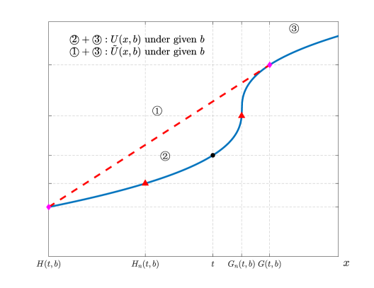
Figure 3: Illustration for functions $G$, $H$, $G_{n}$ and $H_{n}$

B.3 Proof of Theorem 2

We prove Theorem 2 with Assumptions 1 replaced by weaker Assumptions 5 and 6. To prove Theorem 2, we need some further discussion on concavification (Lemma 4) and non-atomic measures. $H_{n}$ and $G_{n}$ are important tools in the proof of Theorem 2, and it is necessary to confirm their measurability before we apply mathematical operations on them, which is stated in the following Lemma 5. Its proof is rather technical.

Lemma 5.

Under Assumption 5, $\tilde{U}$, $H_{n}$ and $G_{n}$ are measurable functions on $(\mathbb{R}\times E,\mathcal{B}(\mathbb{R})\times\mathcal{E})$.

Proof.

Proof of Lemma 5. (1) For $\tilde{U}$, thanks to Lemma 4, we have

$$\tilde{U}(x,b) =\mathop{\sup\limits_{a\leqslant x\leqslant c}}\limits_{a\not=c}\frac{(x-a)U(c,b)+(c-x)U(a,b)}{c-a} =\sup\limits_{a^{\prime},c^{\prime}\in[0,+\infty]\cap\mathbb{Q}\atop(a^{\prime},c^{\prime})\not=(0,0)}\frac{a^{\prime}U(x+c^{\prime},b)+c^{\prime}U(x-a^{\prime},b)}{a^{\prime}+c^{\prime}},$$

which indicates that $\tilde{U}$ is measurable.

(2) Define $A_{1}=\{(t,b):H_{n}(t,b)<s\}$ and

$$A_{2}=\big{\{}(t,b)\in\mathbb{R}\times E:t\geqslant s\text{~{}and~{}}\tilde{U}(x,b)>U(x,b)+\frac{1}{n}~{}\text{for every}~{}x\in[s,t]\big{\}}\cup((-\infty,s)\times E).$$

We first show that $A_{1}=A_{2}$. It is obvious that $A_{1}\subset A_{2}$, and we prove $A_{2}\subset A_{1}$. As $t<s$ leads to $H_{n}(t,b)<s$, it suffices to consider the case that $t\geqslant s$. If $\tilde{U}(x,b)>U(x,b)+\frac{1}{n}~{}\text{holds for every}~{}x\in[s,t]$, then $s>\underline{x}_{b}$, and by definition of $H_{n}$ we know $H_{n}(t,b)\leqslant s$, and when the equality holds, we have $x_{k}\uparrow s$ satisfying $\tilde{U}(x_{k},b)\leqslant U(x_{k},b)+\frac{1}{n}$. Therefore, we derive a contradiction that $\tilde{U}(s,b)>U(s,b)+\frac{1}{n}\geqslant\varlimsup\limits_{x_{k}\uparrow s}U(x_{k},b)+\frac{1}{n}\geqslant\varlimsup\limits_{x_{k}\uparrow s}\tilde{U}(x_{k},b)=\tilde{U}(s,b)$. As such, $A_{2}\subset A_{1}$, and hence $A_{1}=A_{2}$.

Now we investigate the structure of $A_{2}$. Define

$$A_{3}=\big{\{}(t,b):t\geqslant s\text{~{}and~{}}\tilde{U}(x,b)>U(x,b)+\frac{1}{n}~{}\text{for every}~{}x\in[s,t]\big{\}}.$$

We are going to prove

$$A_{3}=\mathop{\bigcup}_{j\geqslant 1}\mathop{\bigcup}_{x\in\mathbb{Q},x\geqslant s}\bigg{(}[s,x]\times\mathop{\bigcap}_{N\geqslant 1}F_{j}\left(z_{1}^{(N)}(x),z_{2}^{(N)}(x),...,z_{N+1}^{(N)}(x)\right)\bigg{)},$$ (34)

where $F_{j}(z_{1},z_{2},...,z_{m})\triangleq\mathop{\bigcap}\limits_{1\leqslant k\leqslant m}\left\{b\in E:~{}\tilde{U}(z_{k},b)>U(z_{k},b)+\frac{1}{n}+\frac{1}{j}\right\}$, and $\left\{z_{i}^{(N)}(x)\right\}_{1\leqslant i\leqslant N+1}$ denotes the $N$-uniform partition points of the interval $[s,x]$. In fact, if we denote the right side of (34) by $A_{4}$, then for $(t,b)\in A_{3}$, we know that $\tilde{U}(x,b)>U(x,b)+\frac{1}{n}$ holds for every $x\in[s,t]$, and hence $t\geqslant s>\underline{x}_{b}$. Define $\theta=\inf\left\{x\in[s,t]:\tilde{U}(x,b)-U(x,b)\right\}$. We have $\{y_{n}\}\subset[s,t]$ satisfying $y_{n}\to y$ and $\tilde{U}(y_{n},b)-U(y_{n},b)\to\theta$. As $\tilde{U}(\cdot,b)$ is continuous on $(\underline{x}_{b},+\infty)$ and that $U(\cdot,b)$ is upper semicontinuous,

$$\theta=\lim_{n\to+\infty}\left(\tilde{U}(y_{n},b)-U(y_{n},b)\right)\geqslant\tilde{U}(y,b)-U(y,b)\geqslant\theta,$$

thus $\theta=\tilde{U}(y,b)-U(y,b)>\frac{1}{n}$, and we have some $j\in\mathbb{N}_{+}~{}s.t.~{}\theta>\frac{1}{n}+\frac{1}{j}$. Again using the continuity of $\tilde{U}(\cdot,b)$ and upper semicontinuity of $U(\cdot,b)$, we know $\tilde{U}(x,b)>U(x,b)+\frac{1}{n}+\frac{1}{2j}$ also holds on $x\in[s,t+\delta]$ for some $\delta>0$, that is, one can find $t^{\prime}\in\mathbb{Q}$ such that $t^{\prime}\geqslant t$ and $[s,t^{\prime}]\times\{b\}\subset A_{3}$. Based on definition of $F_{j}$, we know that $b\in F_{2j}\left(z_{1}^{(N)}(t^{\prime}),z_{2}^{(N)}(t^{\prime}),...,z_{N+1}^{(N)}(t^{\prime})\right)$ for any $N$, thus

$$(t,b)\in[s,t^{\prime}]\times\{b\}\subset[s,t^{\prime}]\times\mathop{\bigcap}_{N\geqslant 1}F_{2j}\left(z_{1}^{(N)}(t^{\prime}),z_{2}^{(N)}(t^{\prime}),...,z_{N+1}^{(N)}(t^{\prime})\right)\subset A_{4},$$

and we know $A_{3}\subset A_{4}$. It suffices to show $A_{4}\subset A_{3}$.

For $(t,b)\in A_{4}$, $(t,b)\in[s,x]\times\mathop{\bigcap}\limits_{N\geqslant 1}F_{j}\left(z_{1}^{(N)}(x),z_{2}^{(N)}(x),...,z_{N+1}^{(N)}(x)\right)$ with some $x\in\mathbb{Q}$ and $j\in\mathbb{N}_{+}$, that is, $s\leqslant t\leqslant x$ and, $\tilde{U}\left(z_{k}^{(N)}(x),b\right)>U\left(z_{k}^{(N)}(x),b\right)+\frac{1}{n}+\frac{1}{j}$ for any $k,~{}N$ satisfying $1\leqslant k\leqslant N+1$. Noting that $\tilde{U}(\cdot,b)$ is continuous and that $U(\cdot,b)$ is right-continuous, we have $\tilde{U}(x,b)\geqslant U(x,b)+\frac{1}{n}+\frac{1}{j}>U(x,b)+\frac{1}{n}$ on $[s,x]\supset[s,t]$. It follows that $A_{4}\subset A_{3}$, which leads to $A_{3}=A_{4}$.

As for a given $z$, $\tilde{U}(z,b)-U(z,b)$ is measurable in $b$, we know $F_{j}\left(z_{1}^{(N)}(x),z_{2}^{(N)}(x),...,z_{N+1}^{(N)}(x)\right)\in\mathcal{E}.$ Therefore, $A_{3}=A_{4}\in\mathcal{B}(\mathbb{R})\times\mathcal{E}$, and $A_{1}=A_{2}=A_{3}\cup((-\infty,s)\times E)$ is also a measurable set, which means that $H_{n}$ is a measurable function. Similarly, one can prove the measurability of $G_{n}$. ∎

At last, for non-atomic measures, we need the following result in Sierpiński (1922):

Lemma 6.

If $\mu$ is a non-atomic measure on $(\Omega,\mathcal{F})$ with $\mu(\Omega)=c$, then there exists a one-parameter family of increasing measurable sets $\{A_{t}\}_{0\leqslant t\leqslant c}$ such that $\mu(A_{t})=t$.

In light of Lemmas 4-6 above, we proceed to prove Theorem 2. The idea is to substitute $X(\omega)$ locally by some $\hat{H}(\omega)$ and $\hat{G}(\omega)$ for some $\omega$ such that $X(\omega)$ does not lie on the concave part of $U$ and $\hat{H}\leqslant X\leqslant\hat{G}$. We proceed to find a proper substitution of $X$ with the form $\hat{X}=\hat{H}\mathds{1}_{C}+\hat{G}\mathds{1}_{D}+X\mathds{1}_{\left(C\cup D\right)^{c}},$ which increases the utility, while the budget value $\mathbb{E}[\xi X]$ keeps unchanged. Figure 3 is provided to assist in understanding. Define

$$H(t,b)=\sup\left\{x\leqslant t:\tilde{U}(x,b)=U(x,b)\right\},G(t,b)=\inf\left\{x\geqslant t:\tilde{U}(x,b)=U(x,b)\right\}.$$

In the following proof, we assume that $H(t,b)$ and $G(t,b)$ are finite, and $\tilde{U}(H(t,b),b)=U(H(t,b),b)>-\infty$, $\tilde{U}(G(t,b),b)=U(G(t,b),b)$ when $\tilde{U}(t,b)>U(t,b)$. Then, based on Lemma 5, we know that $H(t,b)$ and $G(t,b)$ are measurable. Moreover, we define $\hat{H}_{b}=\inf\{t\in\mathbb{R}:H(t,b)<t\}$ and assume $\mathbb{E}\left[\xi\hat{H}_{B}^{-}\right]<+\infty$. These conditions provide a concise proof. For the weaker case with only $H_{n}(t,b)$ and $G_{n}(t,b)$ being finite and Assumption 6, the proof is similar; see also Remark 10.

Proof of Theorem 2..

1. Part I: Let us first assume that the concavification problem is well-defined. It is equivalent to study both problems with binding budget constraints, i.e., $\mathbb{E}[\xi X]=x_{0}$. We are going to prove (9) by contradiction. Suppose

   $$\alpha\triangleq\sup_{X:\mathbb{E}[\xi X]=x_{0}\atop U(X,B)>-\infty}\mathbb{E}[\tilde{U}(X,B)]>\beta\triangleq\sup_{X:\mathbb{E}[\xi X]=x_{0}\atop\tilde{U}(X,B)>-\infty}\mathbb{E}[U(X,B)].$$ (35)

   As such, we have some random variable $X$ satisfying $\mathbb{E}[\xi X]=x_{0}$ and $\mathbb{E}[\tilde{U}(X,B)]>\beta.$ Define

   $$S=\left\{(x,b)\in\mathbb{R}\times E:\tilde{U}(x,b)>U(x,b)\right\},~{}~{}Q=\left\{\omega\in\Omega:(X(\omega),B(\omega))\in S\right\}.$$

   It follows that $\mathbb{P}[Q]>0$. Define two random variables $\hat{H}=H(X,B),~{}\hat{G}=G(X,B).$ On $Q$, we have $\hat{H}<X<\hat{G}$. Hence $\tilde{U}(x,B)$ is affine in $x$ for $\hat{H}<x<\hat{G}$ and $\tilde{U}(x,B)=a_{B}x+c_{B}$, where $a_{B}=\frac{\tilde{U}(\hat{G},B)-\tilde{U}(\hat{H},B)}{\hat{G}-\hat{H}}.$ Based on Lemmas 4 and 5, $a_{B}$ and $c_{B}$ are measurable on $Q$, and $\hat{H}$, $\hat{G}$, $a_{B}$ and $c_{B}$ are finite. In the following Steps 1-3, we desire to construct a new random variable $\hat{X}$ by slightly changing $X$ on $Q$ satisfying $\mathbb{E}[\xi\hat{X}]=x_{0}$ and $\mathbb{E}[U(\hat{X},B)]>\beta$, which is a contradiction.

   Step 1: Take a countable partition of $\mathbb{R}^{5}$ as $\mathbb{R}^{5}=\mathop{\bigcup}_{n\geqslant 1}P_{n},~{}\{P_{n}\}_{n\geqslant 1}\text{ are bounded sets}.$ This leads to a partition of $Q$ as $Q=\mathop{\bigcup}_{n\geqslant 1}Q_{n},~{}Q_{n}\triangleq Q\cap\left\{\omega\in\Omega:(\hat{H},\hat{G},a_{B},c_{B},\xi)\in P_{n}\right\},$ and we proceed to make our substitution of $X$ on every $Q_{n}$ that $\mathbb{P}\left[Q_{n}\right]>0$.

   Step 2: For every $n$ with $\mathbb{P}\left[Q_{n}\right]>0$, we need to determine a partition $Q_{n}=C_{n}\cup D_{n}$ and then we replace $X$ by $\hat{H}$ on the set $C_{n}$ and by $\hat{G}$ on the set $D_{n}$. We need to make sure that the new variable $\hat{X}$ satisfies

   $$\mathbb{E}\left[\xi\hat{X}\mathds{1}_{Q_{n}}\right]=\mathbb{E}\left[\xi X\mathds{1}_{Q_{n}}\right]$$ (36)

   and

   $$\mathbb{E}\left[\tilde{U}(X,B)\mathds{1}_{Q_{n}}\right]\leqslant\mathbb{E}\left[\tilde{U}(\hat{X},B)\mathds{1}_{Q_{n}}\right]=\mathbb{E}\left[U(\hat{X},B)\mathds{1}_{Q_{n}}\right].$$ (37)

   To this end, we denote $p=\mathbb{E}[\xi X\mathds{1}_{Q_{n}}]$. Noting that $\hat{H}$, $\hat{G}$, $a_{B}$, and $\xi$ are bounded on $Q_{n}$, we define $F(t)=\mathbb{E}\left[\xi G\mathds{1}_{\left\{\xi\leqslant ta_{B}\right\}\cap Q_{n}}\right]+\mathbb{E}\big{[}\xi\hat{H}\mathds{1}_{\left\{\xi>ta_{B}\right\}\cap Q_{n}}\big{]},~{}t\geqslant 0.$

   As $\hat{H}<X<G$ holds on $Q$, we have $F(0)=\mathbb{E}\left[\xi\hat{H}\mathds{1}_{Q_{n}}\right]<p$, $F(+\infty)=\mathbb{E}[\xi G\mathds{1}_{Q_{n}}]>p$, and that $F$ is nondecreasing and right-continuous. In the following, we construct $C_{n}$ and $D_{n}$ through two cases such that $\mathbb{E}[\xi(\hat{H}\mathds{1}_{C_{n}}+\hat{G}\mathds{1}_{D_{n}})]=p.$

   • If $F(\sigma)=p$ holds for some $\sigma>0$, we define $C_{n}=\left\{\xi>\sigma a_{B}\right\}\cap Q_{n},~{}D_{n}=\{\xi\leqslant\sigma a_{B}\}\cap Q_{n},$ and then we have $\mathbb{E}\left[\xi(\hat{H}\mathds{1}_{C_{n}}+\hat{G}\mathds{1}_{D_{n}})\right]=F(\sigma)=p$.

   • If $p\notin F(\mathbb{R}_{+})$, we have $\sigma>0$ such that $F(\sigma-)\leqslant p<F(\sigma)$, and then $0<F(\sigma)-F(\sigma-)=\mathbb{E}[\xi(\hat{G}-\hat{H})\mathds{1}_{\{\xi=\sigma a_{B}\}\cap Q_{n}}].$ Hence, the set $Q^{\prime}\triangleq\{\xi=\sigma a_{B}\}\cap Q_{n}$ has a positive measure $\varepsilon$. As $(\Omega,\mathcal{F},\mathbb{P})$ is non-atomic, its restriction on $Q^{\prime}$ is also non-atomic. Using Lemma 6, we obtain a family of increasing measurable sets $\{Q_{t}^{\prime}\}_{0\leqslant t\leqslant\varepsilon}$ satisfying $\mathbb{P}[Q_{t}^{\prime}]=t$ and $Q_{t}^{\prime}\subset Q^{\prime}$. Define $F_{1}(t)=\mathbb{E}[\xi(\hat{G}-\hat{H})\mathds{1}_{Q_{t}^{\prime}}]$. It is verified that $F_{1}$ is nondecreasing and continuous, and $F_{1}(0)=0,~{}F_{1}(\varepsilon)=F(\sigma)-F(\sigma-)\geqslant F(\sigma)-p.$ As such, one can find $\sigma_{1}$ such that $F_{1}(\sigma_{1})=F(\sigma)-p$. In this case we define $C_{n}=\left(\{\xi>\sigma a_{B}\}\cap Q_{n}\right)\cup Q_{\sigma_{1}}^{\prime},~{}D_{n}=\left(\{\xi\leqslant\sigma a_{B}\}\cap Q_{n}\right)\backslash Q_{\sigma_{1}}^{\prime},$ which leads to

     $$\mathbb{E}\left[\xi(\hat{H}\mathds{1}_{C_{n}}+\hat{G}\mathds{1}_{D_{n}})\right] =\mathbb{E}\left[\xi\hat{H}\mathds{1}_{\{\xi>\sigma a_{B}\}\cap Q_{n}}\right]+\mathbb{E}\left[\xi\hat{H}\mathds{1}_{Q_{\sigma_{1}}^{\prime}}\right]+\mathbb{E}\left[\xi\hat{G}\mathds{1}_{\{\xi\leqslant\sigma a_{B}\}\cap Q_{n}}\right]-\mathbb{E}\left[\xi\hat{G}\mathds{1}_{Q_{\sigma_{1}}^{\prime}}\right]$$

     $$=F(\sigma)-F_{1}(\sigma_{1})=p.$$

   Define $\hat{X}=\hat{H}\mathds{1}_{C_{n}}+\hat{G}\mathds{1}_{D_{n}}$ on $Q_{n}$, and then (36) holds. Moreover, as $\hat{H}\leqslant\hat{X}\leqslant\hat{G}$ and $\hat{H}\leqslant X\leqslant\hat{G}$, they are bounded on $Q_{n}$. Hence $\tilde{U}(X,B)=a_{B}X+c_{B}$ and $\tilde{U}(\hat{X},B)=a_{B}\hat{X}+c_{B}$ are also bounded on $Q_{n}$. In both two cases we have

   $$\mathbb{E}\left[\left(\tilde{U}\left(\hat{X},B\right)-\tilde{U}\left(X,B\right)\right)\mathds{1}_{Q_{n}}\right]=\mathbb{E}\left[a_{B}(\hat{G}-X)\mathds{1}_{D_{n}}\right]-\mathbb{E}\left[a_{B}(X-\hat{H})\mathds{1}_{C_{n}}\right]$$

   $$\geqslant \mathbb{E}\left[\frac{\xi}{\sigma}(\hat{G}-X)\mathds{1}_{D_{n}}\right]-\mathbb{E}\left[\frac{\xi}{\sigma}(X-\hat{H})\mathds{1}_{C_{n}}\right]=\frac{1}{\sigma}\mathbb{E}\left[\xi\left(\hat{X}-X\right)\mathds{1}_{Q_{n}}\right]=0,$$

   and hence (37) holds.

   Step 3: For every $n$ with $\mathbb{P}[Q_{n}]=0$, we set $C_{n}=Q_{n}$, $D_{n}=\emptyset$. Define $C=\mathop{\bigcup}_{n\geqslant 1}C_{n},~{}D=\mathop{\bigcup}_{n\geqslant 1}D_{n}.$ Then $C\cup D=Q$ is a partition of $Q$. Define $\hat{X}=\hat{H}\mathds{1}_{C}+\hat{G}\mathds{1}_{D}+X\mathds{1}_{Q^{c}},$ which is consistent with our definition in Step 2. Using (36), we have

   $$\mathbb{E}\left[\xi X\right] =\mathbb{E}\left[\xi X\mathds{1}_{Q^{c}}\right]+\sum\limits_{n\geqslant 1}\mathbb{E}\left[\xi X\mathds{1}_{Q_{n}}\right]=\mathbb{E}\left[\xi\hat{X}\mathds{1}_{Q^{c}}\right]+\sum\limits_{n\geqslant 1}\mathbb{E}\left[\xi\hat{X}\mathds{1}_{Q_{n}}\right]$$ (38)

   $$=\mathbb{E}\left[\xi\hat{X}^{+}\mathds{1}_{Q^{c}}\right]-\mathbb{E}\left[\xi\hat{X}^{-}\mathds{1}_{Q^{c}}\right]+\sum\limits_{n\geqslant 1}\left(\mathbb{E}\left[\xi\hat{X}^{+}\mathds{1}_{Q_{n}}\right]-\mathbb{E}\left[\xi\hat{X}^{-}\mathds{1}_{Q_{n}}\right]\right).$$

   As $\hat{H}<X$ on $Q$, based on the definition of $\hat{H}$, for any $t$ satisfying $\hat{H}<t<X$, we have $H(t,B)=\hat{H}<t$. Based on the definition of $\hat{H}_{b}$, we know $\hat{H}_{B}\leqslant t$. Hence $\hat{H}_{B}\leqslant\hat{H}$ and we have $\hat{X}\geqslant\hat{H}\geqslant\hat{H}_{B}$ on $Q$. Hence $\mathbb{E}\left[\xi\hat{X}^{-}\mathds{1}_{Q}\right]\leqslant\mathbb{E}\left[\xi\hat{H}_{B}^{-}\mathds{1}_{Q}\right]<+\infty,$ and the series $\sum\limits_{n\geqslant 1}\mathbb{E}\left[\xi\hat{X}^{-}\mathds{1}_{Q_{n}}\right]$ converges. As such, (38) indicates that the series $\sum\limits_{n\geqslant 1}\mathbb{E}\left[\xi\hat{X}^{+}\mathds{1}_{Q_{n}}\right]$ also converges, and we have

   $$\mathbb{E}[\xi\hat{X}]=\mathbb{E}[\xi X]=x_{0}.$$ (39)

   Moreover, based on Lemma 4, we know $U(\hat{X},B)>-\infty$, and then (3) indicates that the expectation $\mathbb{E}\left[U(\hat{X},B)\right]$ is well-defined. Using (37), we have (noting that $X=\hat{X}$ and $\tilde{U}(X,B)=U(X,B)$ on $Q^{c}$)

   $$\mathbb{E}\left[\tilde{U}\left(X,B\right)\right] =\mathbb{E}\left[\tilde{U}\left(X,B\right)\mathds{1}_{Q^{c}}\right]+\sum\limits_{n\geqslant 1}\mathbb{E}\left[\tilde{U}\left(X,B\right)\mathds{1}_{Q_{n}}\right]$$

   $$\leqslant\mathbb{E}\left[U\left(\hat{X},B\right)\mathds{1}_{Q^{c}}\right]+\sum\limits_{n\geqslant 1}\mathbb{E}\left[U\left(\hat{X},B\right)\mathds{1}_{Q_{n}}\right]=\mathbb{E}\left[U\left(\hat{X},B\right)\right].$$

   Therefore, $\mathbb{E}\left[U\left(\hat{X},B\right)\right]\geqslant\mathbb{E}\left[\tilde{U}\left(X,B\right)\right]>\beta$, which contradicts to the definition (35) of $\beta$.

   Part II: We are going to prove that the concavification problem is well-defined. For $X$ satisfying $\mathbb{E}\left[\xi X\right]\leqslant x_{0}$ and $\tilde{U}\left(X,B\right)>-\infty$ (which is equivalent to $U\left(X,B\right)>-\infty$), we have that (3) holds with $U$ replaced by $\tilde{U}$. Noting that $\tilde{U}\geqslant U$, if $\mathbb{E}\left[U\left(X,B\right)^{-}\right]<+\infty$, we have immediately $\mathbb{E}\left[\tilde{U}\left(X,B\right)^{-}\right]<+\infty$. It remains to consider the situation where $\mathbb{E}\left[U\left(X,B\right)^{+}\right]<+\infty$. We discuss two cases:

   • If $\tilde{U}\left(X,B\right)^{+}=U\left(X,B\right)^{+}~{}\text{a.s.}$, then $\mathbb{E}\left[\tilde{U}\left(X,B\right)^{+}\right]<+\infty$.

   • If $\mathbb{P}\left[\tilde{U}\left(X,B\right)^{+}>U\left(X,B\right)^{+}\right]>0$, let us consider the two functions $\tilde{h}=\tilde{U}\left(\cdot,b\right)^{+}$ and $h=U\left(\cdot,b\right)^{+}$ for any given $b\in E$. Based on Lemmas 4 and 5, we have:

     • For $a,c\in\mathbb{R}$ and $a<c$, if $\tilde{h}>h$ on $(a,c)$, then $\tilde{h}$ is affine on $(a,c)$.

     • For $t\in\mathbb{R}$, define $\begin{aligned} H^{*}(t)=\sup\{x\leqslant t:\tilde{h}(x)=h(x)\},~{}G^{*}(t)=\inf\{x\geqslant t:\tilde{h}(x)=h(x)\}.\end{aligned}$ If $\tilde{h}(t)>h(t)$, then $G^{*}(t)$ and $H^{*}(t)\in\mathbb{R}$, and $\tilde{h}(G^{*}(t))=h(G^{*}(t))\in\mathbb{R}$, $\tilde{h}(H^{*}(t))=h(H^{*}(t))\in\mathbb{R}$, and then $H(t)\leqslant H^{*}(t)<t<G^{*}(t)\leqslant G(t)$, where $H(t)$ and $G(t)$ are defined in Lemma 4.

     Define $S^{+}=\left\{(x,b)\in\mathbb{R}\times E:\tilde{U}(x,b)^{+}>U(x,b)^{+}\right\},~{}~{}Q^{+}=\left\{\omega\in\Omega:(X(\omega),B(\omega))\in S^{+}\right\}.$ Then $\mathbb{P}[Q^{+}]>0$. Using the above two features, we can replicate our operations in Part I to construct $Q_{n}^{+}=C_{n}^{+}\cup D_{n}^{+}$ and $\hat{X}=\hat{H}^{*}\mathds{1}_{C^{+}}+\hat{G}^{*}\mathds{1}_{D^{+}}+X\mathds{1}_{Q^{+c}}$ with

     $$\hat{H}^{*}\triangleq H^{*}(X,B),~{}\hat{G}^{*}\triangleq G^{*}(X,B),~{}C^{+}\triangleq\mathop{\bigcup}_{n\geqslant 1}C_{n}^{+},~{}D^{+}\triangleq\mathop{\bigcup}_{n\geqslant 1}D_{n}^{+},~{}Q^{+}=\mathop{\bigcup}_{n\geqslant 1}Q_{n}^{+}.$$

     On each $Q_{n}^{+}$ with $\mathbb{P}\left[Q_{n}^{+}\right]>0$, we have $\mathbb{E}[\xi\hat{X}\mathds{1}_{Q_{n}^{+}}]=\mathbb{E}[\xi X\mathds{1}_{Q_{n}^{+}}]$ and

     $$\mathbb{E}\left[\tilde{U}(X,B)^{+}\mathds{1}_{Q_{n}^{+}}\right]\leqslant\mathbb{E}\left[\tilde{U}(\hat{X},B)^{+}\mathds{1}_{Q_{n}^{+}}\right]=\mathbb{E}\left[U(\hat{X},B)^{+}\mathds{1}_{Q_{n}^{+}}\right].$$ (40)

     As discussed in Step 3, we have $\mathbb{E}\left[\xi\hat{X}\right]=\mathbb{E}\left[\xi X\right]\leqslant x_{0}$. Using (3), we have

     $$\mathbb{E}\left[U(\hat{X},B)^{+}\right]<+\infty\text{ or }\mathbb{E}\left[U(\hat{X},B)^{-}\right]<+\infty.$$

     If $\mathbb{E}\left[U(\hat{X},B)^{+}\right]<+\infty$, then, using (40), we have $\mathbb{E}\left[\tilde{U}(X,B)^{+}\right]<+\infty$.

     If $\mathbb{E}\left[U(\hat{X},B)^{-}\right]<+\infty$, then as $\tilde{U}\geqslant U$, we have $\mathbb{E}\left[\tilde{U}(\hat{X},B)^{-}\right]<+\infty$.
     Noting that on $C^{+}\cup D^{+}=Q^{+}$, we have $\tilde{U}\left(X,B\right)^{+}>U\left(X,B\right)^{+}\geqslant 0$. Hence $\tilde{U}\left(X,B\right)^{-}=0$, and we have $\mathbb{E}\left[\tilde{U}\left(X,B\right)^{-}\mathds{1}_{Q^{+}}\right]=0,~{}\mathbb{E}\left[\tilde{U}\left(X,B\right)^{-}\mathds{1}_{Q^{+c}}\right]=\mathbb{E}\left[\tilde{U}\left(\hat{X},B\right)^{-}\mathds{1}_{Q^{+c}}\right]<+\infty,$ which indicates that $\mathbb{E}\left[\tilde{U}(X,B)^{-}\right]<+\infty$. Therefore, the concavification problem is well-defined.

2. Suppose that $X^{*}$ is a finite optimal solution of Problem (2). We have

   $$\mathbb{E}\left[\tilde{U}\left(X^{*},B\right)\right]\geqslant\mathbb{E}\left[U\left(X^{*},B\right)\right]=\sup_{X:\mathbb{E}[\xi X]=x_{0}\atop U(X,B)>-\infty}\mathbb{E}\left[U(X,B)\right]=\sup_{X:\mathbb{E}[\xi X]=x_{0}\atop\tilde{U}(X,B)>-\infty}\mathbb{E}\left[\tilde{U}(X,B)\right].$$

   As such, $X^{*}$ is also an optimal solution for $\sup_{X:\mathbb{E}[\xi X]=x_{0}\atop\tilde{U}(X,B)>-\infty}\mathbb{E}\left[\tilde{U}(X,B)\right]$, and

   $$\mathbb{E}\left[\tilde{U}(X^{*},B)\right]=\mathbb{E}[U(X^{*},B)]\in\mathbb{R},$$

   that is, $\tilde{U}(X^{*},B)=U(X^{*},B)$ a.s.. Applying Theorem 1, $X^{*}\in\mathcal{X}_{B}^{\tilde{U}}(\lambda\xi)$ for some $\lambda\geqslant 0$.

   • When $\lambda<+\infty$, we obtain $X^{*}\in\mathcal{X}_{B}^{U}(\lambda\xi)$ from

     $$U(X^{*},B)-\lambda\xi X^{*}=\tilde{U}(X^{*},B)-\lambda\xi X^{*}\geqslant\tilde{U}(x,B)-\lambda\xi x\geqslant U(x,B)-\lambda\xi x,~{}\forall x\in\mathbb{R}.$$

   • When $\lambda=+\infty$, we have $X^{*}=\underline{x}_{B}^{\tilde{U}}=\underline{x}_{B}^{U}$ (based on Lemma 4). Hence, $X^{*}\in\mathcal{X}_{B}^{U}(\lambda\xi)$.

   Conversely, if there exists $X^{*}\in\mathcal{X}_{B}^{U}(\lambda\xi)$ satisfying $\mathbb{E}[\xi X^{*}]=x_{0}$ and $U(X^{*},B)>-\infty$, then:

   • If $\lambda<+\infty$. For any other $X$ satisfying the budget constraint and $U(X,B)>-\infty$, we have

     $$U(X^{*},B)-\lambda\xi X^{*}\geqslant U(X,B)-\lambda\xi X>-\infty.$$

     Taking the expectation on both sides, we obtain $\mathbb{E}[U(X^{*},B)]\geqslant\mathbb{E}[U(X,B)]$, as such,

     $$\mathbb{E}[U(X^{*},B)]\geqslant\sup_{X:\mathbb{E}[\xi X]=x_{0}\atop U(X,B)>-\infty}\mathbb{E}[U(X,B)]\geqslant\mathbb{E}[U(X^{*},B)].$$

     Thus, $X^{*}$ is an optimal solution of Problem (2).

   • If $\lambda=+\infty$, then $X^{*}=\underline{x}_{B}$. As $U(X,B)>-\infty$ requires $X\geqslant\underline{x}_{B}=X^{*}$, we have $\mathbb{E}\left[\xi X\right]\geqslant\mathbb{E}\left[\xi X^{*}\right]=x_{0}$. This indicates that $X^{*}$ is the unique random variable satisfying the constraint in Problem (2), and hence $X^{*}$ is the optimal solution.

   Note that in this part we do not need the non-atomic condition. The proof is also valid for the “if” part in Theorem 1.

∎

Remark 10.

For the weaker case with only $H_{n}$ and $G_{n}$ being finite, we should take some $m\in\mathbb{N}_{+}$ in Part I with $\mathbb{E}[\tilde{U}(X,B)]>\beta+\frac{1}{m}.$ And then we make our operation on the set $S=\big{\{}(x,b)\in\mathbb{R}\times E:\tilde{U}(x,b)>U(x,b)+\frac{1}{m}\big{\}}$ and replace $X$ by $H_{2m}(X,B)$ and $G_{2m}(X,B)$.

Appendix C Proofs in Section 4

C.1 Proof of Lemma 1

To prove Lemma 1, we need:

Lemma 7.

Suppose that $u:\mathbb{R}\to\mathbb{R}\cup\{-\infty\}$ proper with a concavification $\tilde{u}:\mathbb{R}\to\mathbb{R}\cup\{-\infty\}$. Then for $y\in(0,+\infty)$ we have $\mathcal{X}^{u}(y)\subset\mathcal{X}^{\tilde{u}}(y)$, where the term is defined as in (6) with $b$ omitted.

Proof of Lemma 7..

Denote by $f^{*}(y)$ the convex conjugate of $f$, i.e. $f^{*}(y)=\sup_{x\in\mathbb{R}}\{xy-f(x)\}.$ Then we have $\tilde{u}=-(-u)^{**}$ (cf. Rockafellar (1970)). Using the Fenchel-Moreau Theorem, we know

$$V(y)\triangleq\sup_{x\in\mathbb{R}}\{\tilde{u}(x)-xy\}=\sup_{x\in\mathbb{R}}\{x(-y)-(-u)^{**}(x)\}=(-u)^{***}(-y)=(-u)^{*}(-y)=\sup_{x\in\mathbb{R}}\{u(x)-xy\}.$$

For $x\in\mathcal{X}^{u}(y)$, we consider three cases:

1. $x\in\mathbb{R}$. In this case, we have $\tilde{u}(x)-xy\geqslant u(x)-xy=\sup_{t\in\mathbb{R}}\{u(t)-ty\}=\sup_{t\in\mathbb{R}}\{\tilde{u}(t)-ty\}.$ Hence $x\in\mathcal{X}^{\tilde{u}}(y)$.

2. $x=+\infty$. Then there exists $x_{n}\uparrow+\infty$ with $u(x_{n})-x_{n}y\to\sup_{x\in\mathbb{R}}\{u(x)-xy\}=V(y)$. As $V(y)\geqslant\tilde{u}(x_{n})-x_{n}y\geqslant u(x_{n})-x_{n}y$, we know $\tilde{u}(x_{n})-x_{n}y\to V(y)$. Hence $+\infty\in\mathcal{X}^{\tilde{u}}(y)$.

3. $x=-\infty$. The proof is similar as in (ii).

∎

Proof of Lemma 1..

As in this lemma, only (iii) is relevant to $b$. For simplicity, we will first prove (i)(ii)(iv)(v) omitting the notation of $b$, and then prove (iii). Also, as terms in the lemma may equal $\pm\infty$, we will prove by contradiction.

(i) Suppose $x^{*}\triangleq\underline{X}(y)<\underline{x}$ for some $y\in\left[0,+\infty\right]$, then $\underline{x}>-\infty$. As $\mathcal{X}(+\infty)=\{\underline{x}\}$, we know $y<+\infty$. Hence there exists a sequence of real numbers $\{x_{n}\}\downarrow x^{*}$ with $U(x_{n})-x_{n}y\to V(y)$. However, for $x_{n}$ closed enough to $x^{*}$ we have $x_{n}<\underline{x}$, which means $U(x_{n})=-\infty$. Hence $V(y)=-\infty$, which contradicts to Assumption 1.

Suppose $x^{**}\triangleq\overline{X}(y)>\overline{x}$ for some $y\in(0,+\infty]$, then $\overline{x}<+\infty$. As $\overline{x}\geqslant\underline{x}$, we know $y<+\infty$. Hence there exists a sequence of real numbers $\{x_{n}\}\uparrow x^{**}$ with $U(x_{n})-x_{n}y\to V(y)$. However, for $x_{n}$ closed enough to $x^{**}$ we have $x_{n}>\overline{x}$, which means $U(x_{n})=U(\overline{x})$. As such, $U(x_{n})-x_{n}y=U(\overline{x})-x_{n}y\to U(\overline{x})-x^{**}y$. That is, $V(y)=U(\overline{x})-x^{**}y<U(\overline{x})-\overline{x}y$, which contradicts to the definition (5) of $V$.

(ii) Step 1: We prove $x^{*}\triangleq\underline{X}(y)\in\mathcal{X}(y)$.

For $y=+\infty$, we have $\mathcal{X}(y)=\{\underline{x}\}$. Hence $\underline{X}(y)=\overline{X}(y)=\underline{x}\in\mathcal{X}(y)$.

For $y\in[0,+\infty)$, we have a sequence of real numbers $\{x_{n}\}\downarrow$ (or $\uparrow$) $x^{*}$ with $U(x_{n})-x_{n}y\to V(y)$. If $x^{*}\in\{\pm\infty\}$, then by the definition (6) of $\mathcal{X}(y)$ we know $x^{*}\in\mathcal{X}(y)$. If $x^{*}\in\mathbb{R}$, then it follows from the upper semicontinuity of $U$ that $V(y)=\lim_{n\to+\infty}U(x_{n})-x^{*}y\leqslant U(x^{*})-x^{*}y.$ Based on the definition (5) of $V$, we know $V(y)=U(x^{*})-x^{*}y$, i.e. $x^{*}\in\mathcal{X}(y)$. Similarly, we have $\overline{X}(y)\in\mathcal{X}(y)$.

Step 2: We prove $\overline{X}(y_{2})\leqslant\underline{X}(y_{1})$ for $0\leqslant y_{1}<y_{2}\leqslant+\infty$.

If $y_{2}=+\infty$, then $\overline{X}(y_{2})=\underline{x}\leqslant\underline{X}(y_{1})$ (using (i) above).

If $y_{2}<+\infty$, suppose that we have $0\leqslant y_{1}<y_{2}$ such that $x^{**}\triangleq\overline{X}(y_{2})>x^{*}\triangleq\underline{X}(y_{1})$. We have a sequence of real numbers $\{x_{n}\}\downarrow$ (or $\uparrow$) $x^{*}$ with $U(x_{n})-x_{n}y_{1}\to V(y_{1})$, and a sequence of real numbers $\{x_{n}^{\prime}\}\downarrow$ (or $\uparrow$) $x^{**}$ with $U(x_{n}^{\prime})-x_{n}^{\prime}y_{2}\to V(y_{2})$, and we can assume

$$\left\{\begin{aligned} &U(x_{n})-x_{n}y_{1}>V(y_{1})-1/n\geqslant U(x_{n}^{\prime})-x_{n}^{\prime}y_{1}-1/n,\\ &U(x_{n}^{\prime})-x_{n}^{\prime}y_{2}>V(y_{2})-1/n\geqslant U(x_{n})-x_{n}y_{2}-1/n.\end{aligned}\right.$$ (41)

As $x^{**}>x^{*}\geqslant\underline{x}$, for $n$ sufficiently large we have $x_{n}^{\prime}>\underline{x}$ and $U(x_{n}^{\prime})\in\mathbb{R}$. Then the first inequality in (41) indicates $U(x_{n})\in\mathbb{R}$, and we can add two inequalities in (41) to derive $(x_{n}-x_{n}^{\prime})(y_{2}-y_{1})\geqslant\frac{2}{n}.$ Letting $n\to+\infty$, as $x_{n}-x_{n}^{\prime}\to x^{*}-x^{**}<0$, we obtain a contradiction.

(iii) Based on (ii), for $0\leqslant y_{1}<y_{2}\leqslant+\infty$, we have $\underline{X}(y_{2})\leqslant\overline{X}(y_{2})\leqslant\underline{X}(y_{1})\leqslant\overline{X}(y_{1})$. The proof of the measurability will be given at the last of the proof. (iv) Because of the nonincreasing property just shown in (iii), both two limits exist (including the limit to infinity).

Step 1: We prove $l\triangleq\lim\limits_{y\to 0+}\overline{X}(y)=\overline{x}$.

If $l\in\mathbb{R}$, then there exist real numbers $y_{n}\downarrow 0$ and $x_{n}\uparrow l$ such that $\overline{X}(y_{n})=x_{n}\in\mathcal{X}(y_{n})$. As such,

$$U(l)-x_{n}y_{n}\geqslant U(x_{n})-x_{n}y_{n}\geqslant U(x)-xy_{n},\text{ for any }x\in\mathbb{R}.$$ (42)

Letting $n\to+\infty$, (42) leads to $U(l)\geqslant U(x)$, and we have $\overline{x}\leqslant l$. Using (i) we know $l=\overline{x}$. If $l=+\infty$, it follows from (i) that $+\infty\leqslant\overline{x}$, and hence $\overline{x}_{b}=+\infty=l$.

If $l=-\infty$, then for any $y\in(0,+\infty)$ we have $\overline{X}(y)=-\infty$. Using Lemma 7, we know $-\infty\in\mathcal{X}^{U}(y)\subset\mathcal{X}^{\tilde{U}}(y)$. As $\tilde{U}$ is concave, we have $\tilde{U}^{\prime}(-\infty)\leqslant y$ for every $y>0$. Noting that $\tilde{U}$ is nondecreasing, $\tilde{U}^{\prime}(-\infty)\geqslant 0$, we derive $\tilde{U}^{\prime}(-\infty)=0$. This indicates that $\tilde{U}$ is constant on $\mathbb{R}$. Based on the assumption that $U\in\mathcal{H}$, we know that $U$ is also constant on $\mathbb{R}$. Therefore, $\underline{x}=\overline{x}=-\infty=l$.

Similarly, we can prove $\lim\limits_{y\to 0+}\underline{X}(y)=\overline{x}$. Step 2: We prove $L\triangleq\lim\limits_{y\to+\infty}\overline{X}(y)=\underline{x}$. Suppose that $L>\underline{x}$, then $L>-\infty$ and $U(L-)>-\infty$.

If $L\in\mathbb{R}$, there exist real numbers $y_{n}\uparrow+\infty$ and $x_{n}\downarrow L$ such that $\overline{X}(y_{n})=x_{n}$. For any $x\in\mathbb{R}$,

$$U(x_{n})-x_{n}y_{n}\geqslant U(x)-xy_{n}.$$ (43)

For $v>0$, we take $x=x_{n}-\frac{v}{y_{n}}>\underline{x}$ for some large $n$, and (43) yields $\begin{aligned} U(x_{n})\geqslant U(x_{n}-\frac{v}{y_{n}})+v.\end{aligned}$ Letting $n\to+\infty$, we obtain $\begin{aligned} U(L)\geqslant U(L-)+v,\end{aligned}$ which is a contradiction as $v$ is arbitrary. Thus $L$ cannot be larger than $\underline{x}$. As $L\geqslant\underline{x}$ we know $L=\underline{x}$. If $L=+\infty$, then for any $y\in[0,+\infty)$, we have $\overline{X}(y)=+\infty\in\mathcal{X}^{\tilde{U}}(y)$. As such, $\tilde{U}^{\prime}(+\infty)\geqslant y$ for every $y<+\infty$, which contradicts to the fact that $\tilde{U}$ is concave.

In conclusion, $L=\underline{x}$. Similarly, we can prove $\lim\limits_{y\to+\infty}\underline{X}(y)=\underline{x}$. (v) Step 1: We prove $l\triangleq\lim\limits_{y\to y_{0}+}\overline{X}(y)=\underline{X}(y_{0})$. Suppose $l<\underline{X}(y_{0})$, which implies $l<+\infty$.

If $l\in\mathbb{R}$, again we have real numbers $y_{n}\downarrow y_{0}$ as well as $x_{n}=\overline{X}(y_{n})\uparrow l$ satisfying (42). When $n$ tends to infinity, the inequality shows that for any $x\in\mathbb{R}$, $\begin{aligned} U(l)-ly_{0}\geqslant U(x)-xy_{0},\end{aligned}$ which means $l\in\mathcal{X}(y_{0})$. As such, $l\geqslant\underline{X}(y_{0})$, which is a contradiction.

If $l=-\infty$, then for any $y\in(y_{0},+\infty)$ we have $\overline{X}(y)=-\infty$. As we have discussed in (iv), this indicates $\tilde{U}^{\prime}(-\infty)\leqslant y$ for any $y>y_{0}$, i.e., $\tilde{U}^{\prime}(-\infty)\leqslant y_{0}$. Let us discuss several cases.

(a) If $l^{\prime}\triangleq\underline{X}(y_{0})\in\mathbb{R}$, and for any $x<l^{\prime}$, we have $U(x)=\tilde{U}(x)$.

In this case, for $x<l^{\prime}$ we have $U(x)-xy_{0}=\tilde{U}(x)-xy_{0}\geqslant\tilde{U}(l^{\prime})-l^{\prime}y_{0}\geqslant U(l^{\prime})-l^{\prime}y_{0}=V(y_{0}),$ which means $x\in\mathcal{X}(y_{0})$. This contradicts to the definition of $\underline{X}(y_{0})$ and the fact $x<l^{\prime}$.

(b) If $l^{\prime}\in\mathbb{R}$, and there exists $x<l^{\prime}$ such that $U(x)<\tilde{U}(x)$.

As $U\in\mathcal{H}$, there exists a nonincreasing sequence $\{x_{k}^{\prime}\}$ with $x_{k}^{\prime}\leqslant x$ and $\tilde{U}(x_{k}^{\prime})<U(x_{k}^{\prime})+\frac{1}{k}$. As such, for $l^{\prime}>x\geqslant x_{k}^{\prime}$, using the fact $\tilde{U}^{\prime}(-\infty)\leqslant y_{0}$, we have

$$U(x_{k}^{\prime})-x_{k}^{\prime}y_{0}+\frac{1}{k}>\tilde{U}(x_{k}^{\prime})-x_{k}^{\prime}y_{0}\geqslant\tilde{U}(l^{\prime})-l^{\prime}y_{0}\geqslant U(l^{\prime})-l^{\prime}y_{0}=V(y_{0}).$$

Letting $k\to+\infty$, we know $\lim\limits_{k\to+\infty}x_{k}^{\prime}\in\mathcal{X}(y_{0})$, which is also a contradiction because $\lim\limits_{k\to+\infty}x_{k}^{\prime}<l^{\prime}$.

(c) If $l^{\prime}=+\infty$. In this case we have $x_{k}^{\prime\prime}$ increasing to $+\infty$ with $U(x_{k}^{\prime\prime})-x_{k}^{\prime\prime}y_{0}>V(y_{0})-\frac{1}{k}$. Fix $x\in\mathbb{R}$, using the nonincreasing sequence $\{x_{k}^{\prime}\}$ in (b), we derive for $k$ sufficiently large that

$$U(x_{k}^{\prime})-x_{k}^{\prime}y_{0}+\frac{1}{k}>\tilde{U}(x_{k}^{\prime})-x_{k}^{\prime}y_{0}\geqslant\tilde{U}(x_{k}^{\prime\prime})-x_{k}^{\prime\prime}y_{0}\geqslant U(x_{k}^{\prime\prime})-x_{k}^{\prime\prime}y_{0}>V(y_{0})-\frac{1}{k}.$$

Letting $k\to+\infty$, we know $\lim\limits_{k\to+\infty}x_{k}^{\prime}\in\mathcal{X}(y_{0})$, which is also a contradiction because $\lim\limits_{k\to+\infty}x_{k}^{\prime}\leqslant x<l^{\prime}$.

Concluding (a)-(c), we have proved $l^{\prime}=-\infty=l$. Step 2: We prove $L\triangleq\lim\limits_{y\to y_{0}-}\underline{X}(y)=\overline{X}(y_{0})$. Suppose $L>\overline{X}(y_{0})$, then $L>-\infty$.

If $L\in\mathbb{R}$, the proof is all the same as in Step 1.

If $L=+\infty$, then for any $y\in[0,y_{0})$ we have $\underline{X}(y)=+\infty$. As we have discussed in (iv), this indicates $\tilde{U}^{\prime}(+\infty)\geqslant y$ for any $y\in[0,y_{0})$, i.e., $\tilde{U}^{\prime}(+\infty)\geqslant y_{0}$. Using the same method in Step 1, we can prove $L^{\prime}\triangleq\overline{X}(y_{0})=+\infty=L$.

(iii) At last, we prove the measurability of $V_{b}(y),~{}\underline{X}_{b}(y)$ and $\overline{X}_{b}(y)$.

Step 1: We prove that $V_{b}(y)$ is measurable.

Note that $U(\cdot,b)$ is nondecreasing. For $t\in\mathbb{R}$, $V_{b}(y)\leqslant t$ is equivalent to $U(x,b)-xy\leqslant t$ for all $x\in\mathbb{Q}$. That is, $(y,b)\in\mathop{\bigcap}\limits_{x\in\mathbb{Q}}S_{x},$ where $S_{x}=\left\{(y,b)\in[0,+\infty)\times E:U(x,b)-xy\leqslant t\right\}.$ For given $x$, as $U(x,b)$ is a measurable function of $b$, we know that $U(x,b)-xy$ is a measurable function of $(y,b)$ and $S_{x}\in\mathcal{B}\left([0,+\infty)\right)\times\mathcal{E}$. Therefore, we obtain $\mathop{\cap}\limits_{x\in\mathbb{Q}}S_{x}\in\mathcal{B}\left([0,+\infty)\right)\times\mathcal{E}$, which leads to the measurability of $V_{b}(y)$ in $(y,b)$.

Step 2: We prove that $\underline{X}_{b}(y)$ is measurable. Based on the definition of $\underline{X}_{b}(y)$, for $(y,b)\in[0,+\infty)\times E$ and $t\in\mathbb{R}$ we have:

$$\underline{X}_{b}(y)>t\iff~{}\left\{\begin{aligned} &\exists~{}n\in\mathbb{N}_{+}~{}s.t.~{}U(x,b)-xy\leqslant V_{b}(y)-\frac{1}{n}\text{ holds for all }x\leqslant t,~{}&\text{if }V_{b}(y)<+\infty;\\ &\exists~{}n\in\mathbb{N}_{+}~{}s.t.~{}U(x,b)-xy\leqslant n\text{ holds for all }x\leqslant t,~{}&\text{if }V_{b}(y)=+\infty;\\ \end{aligned}\right.$$ (44)

Noting that in the definition of $\underline{X}_{b}(y)$, $y$ is allowed to be $+\infty$. As such, $\underline{X}_{b}(y)>t$ is equivalent to

$$(y,b)\in\bigg{(}\mathop{\bigcup}_{n\in\mathbb{N_{+}}}\mathop{\bigcap}\limits_{x\in\mathbb{Q}\cup\{t\}\atop x\leqslant t}\widetilde{S}_{x}^{n}\bigg{)}\bigcup\bigg{(}\mathop{\bigcup}_{n\in\mathbb{N_{+}}}\mathop{\bigcap}\limits_{x\in\mathbb{Q}\cup\{t\}\atop x\leqslant t}\widetilde{T}_{x}^{n}\bigg{)}\bigcup W,$$

where

$$\left\{\begin{aligned} &\widetilde{S}_{x}^{n}\triangleq\left\{(y,b)\in[0,+\infty)\times E:U(x,b)-xy\leqslant V_{b}(y)-\frac{1}{n}\right\}\cap\{(y,b)\in[0,+\infty)\times E:V_{b}(y)<+\infty\},\\ &\widetilde{T}_{x}^{n}\triangleq\left\{(y,b)\in[0,+\infty)\times E:U(x,b)-xy\leqslant n\right\}\cap\{(y,b)\in[0,+\infty)\times E:V_{b}(y)=+\infty\},\\ &W=\{+\infty\}\times\{b\in E:\underline{x}_{b}>t\}.\end{aligned}\right.$$

Based on the measurability of $V_{b}(y)$, we know that $U(x,b)-xy-V_{b}(y)$ is measurable in $(y,b)$ for given $x$. Hence $\widetilde{S}_{x}^{n}\in\mathcal{B}\left([0,+\infty)\right)\times\mathcal{E}\subset\mathcal{B}\left([0,+\infty]\right)\times\mathcal{E}$. Similarly, we have $\widetilde{T}_{x}^{n}\in\mathcal{B}\left([0,+\infty]\right)\times\mathcal{E}$. We consider $W$. As $\underline{x}_{b}>t$ is equivalent to $\exists~{}n\in\mathbb{N}_{+}~{}s.t.~{}U(x,b)=-\infty,~{}\forall x\in\mathbb{Q}\cap(-\infty,t+\frac{1}{n}].$ Then

$$\underline{x}_{b}>t\iff b\in\mathop{\bigcup}_{n\in\mathbb{N}_{+}}\mathop{\bigcap}\limits_{x\in\mathbb{Q}\atop x\leqslant t+\frac{1}{n}}\{b\in E:U(x,b)=-\infty\}.$$

As $U(x,\cdot)$ is measurable on $(E,\mathcal{E})$, we know $\{b\in E:\underline{x}_{b}>t\}\in\mathcal{E}$. Hence $W\in\mathcal{B}\left([0,+\infty]\right)\times\mathcal{E}$. Therefore, we know $\left\{(y,b)\in[0,+\infty]\times E:\underline{X}_{b}(y)>t\right\}\in\mathcal{B}\left([0,+\infty]\right)\times\mathcal{E}$, and $\underline{X}_{b}(y)$ is measurable.

Using the same method, one can prove the measurability of $\overline{X}_{b}(y)$.∎

C.2 Proof of Proposition 2

Proof of Proposition 2..

To start with, it is clear that

• If $x_{0}<\mathbb{E}[\xi\underline{x}_{B}]$, then $x_{0}\notin I$;

• If $x_{0}=\mathbb{E}[\xi\underline{x}_{B}]$, $X=\underline{x}_{B}$ is the only possible feasible solution.

• If $x_{0}\geqslant\mathbb{E}[\xi\overline{x}_{B}]$, Problem (2) admits a bliss solution $X\geqslant\overline{x}_{B}$.

The main difficulty appears in the case $\mathbb{E}[\xi\underline{x}_{B}]<x_{0}<\mathbb{E}[\xi\overline{x}_{B}]$. We first prove that the set $I$ is a connected interval, i.e., if $x\in I$, then $[x,+\infty)\subset I$. For $x\in I$, suppose $X$ is a feasible solution with respect to the initial value $x$. Setting $X^{\prime}=X+c\mathds{1}_{\{\xi<n\}}$ for some positive constants $c$ and $n$, one can prove that any $x^{\prime}>x$ is also an element of $I$.

Next, we proceed to prove that if $x\in I$ and $x>\mathbb{E}[\xi\underline{x}_{B}]$, then there exists $x_{1}<x$ such that $[x_{1},+\infty)\subset I$. Suppose that $\mathbb{E}[\xi\underline{x}_{B}]<x=\mathbb{E}[\xi X]$ for some feasible solution $X$. Then we have the set $A_{1}=\{X>\underline{x}_{B}\}\cap\{\xi<N\}$ has a positive probability for some $N>0$. Noting that $\Delta_{x}U(X,B)\triangleq U(X+,B)-U(X-,B)$ is finite and nonnegative on $A_{1}$, we have $A_{2}=\{\Delta_{x}U(X,B)<N_{1}\}\cap\{\xi<N\}$ with $\mathbb{P}[A_{2}]>0$ for some $N_{1}>0$. As $U(\cdot,B)$ is nondecreasing and right-continuous, we rewrite $A_{2}$ as

$$\small A_{2}=\Bigg{(}\mathop{\bigcup}\limits_{n\in\mathbb{N}_{+}}\bigg{\{}U(X,B)-U(X-\frac{1}{n},B)<N_{1}\bigg{\}}\Bigg{)}\bigcap\{\xi<N\}.$$

Therefore, there exists $N_{2}>0$ such that $A\triangleq\big{\{}U(X,B)-U(X-\frac{1}{N_{2}},B)<N_{1}\big{\}}\cap\{\xi<N\}$ has positive probability. Define $X^{\prime}=X-\frac{1}{N_{2}}\mathds{1}_{A}$. Based on the definition of $A$, we know $X^{\prime}\geqslant\underline{x}_{B}$, and $U(X^{\prime},B)>U(X,B)-N_{1}$. As such, $\mathbb{E}[U(X^{\prime},B)]>\mathbb{E}[U(X,B)]-N_{1}>-\infty$. Further, $\mathbb{E}[\xi X^{\prime}]=\mathbb{E}[\xi X]-\frac{1}{N_{2}}\mathbb{E}[\xi\mathds{1}_{A}]$ is a finite number $x_{1}<x$ with $x_{1}\in I$, which also indicates $[x_{1},+\infty)\subset I$.

As a result, we have either $I=[\mathbb{E}[\xi\underline{x}_{B}],+\infty)$ or $I=(\tilde{x},+\infty)$ for some $\tilde{x}\geqslant\mathbb{E}[\xi\underline{x}_{B}]$, where $\tilde{x}$ is allowed to take value in $\{\pm\infty\}$. ∎

C.3 Proof of Theorem 3

We prove Theorem 3 with Assumptions 1 replaced by Assumptions 5 and 6. The proof of Theorem 3 requires the following lemma:

Lemma 8.

For any finite random variable $Y$ in a non-atomic probability space $(\Omega,\mathcal{F},\mathbb{P})$ with $\mathbb{E}[Y^{+}]=+\infty$ and any $a\geqslant 0$, there exists an event $A\in\mathcal{F}$ such that $\mathbb{E}[Y\mathds{1}_{A}]=a$.

Proof of Lemma 8..

It suffices to find $A\in\mathcal{F}$ such that $\mathbb{E}[Y^{+}\mathds{1}_{A}]=a$. Hence we only need to consider the case that $Y\geqslant 0$. Define $F_{1}(t)=\mathbb{E}[Y\mathds{1}_{\{Y<t\}}]$. $F_{1}$ is nondecreasing and left-continuous with $F_{1}(+\infty)=+\infty$. Therefore, we find $t_{1}$ such that $F_{1}(t_{1})>a$. Noting that $(\Omega,\mathcal{F},\mathbb{P})$ is non-atomic, based on Lemma 6, we get a family of increasing measurable sets $\{A_{t}\}_{0\leqslant t\leqslant 1}$ with $\mathbb{P}[A_{t}]=t$. Define $F_{2}(t)=\mathbb{E}[Y\mathds{1}_{A_{t}\cap\{Y<t_{1}\}}]$. $F_{2}$ is continuous with $F_{2}(0)=0$ and $F_{2}(1)=F_{1}(t_{1})>a$. As such, we find $t_{2}\in(0,t_{1})$ satisfying $F_{2}(t_{2})=\mathbb{E}[Y\mathds{1}_{A_{t_{2}}\cap\{Y<t_{1}\}}]=a$. Thus, $A=A_{t_{2}}\cap\{Y<t_{1}\}\in\mathcal{F}$ is the desired set. ∎

Proof of Theorem 3..

1. As $x_{0}>\mathbb{E}[\xi\underline{x}_{B}]$ and $x_{0}\in I$, based on Proposition 2, there admits a feasible solution $X^{\prime}$ for Problem (2) with initial value $x_{1}<x_{0}$.

   For any $\lambda>0$, as $\mathbb{E}[\xi\underline{X}_{B}(\lambda\xi)]=+\infty$, we know that $\mathbb{E}\left[\xi\left(\underline{X}_{B}\left(\lambda\xi\right)-X^{\prime}\right)\right]=+\infty$. Using Lemma 8, we have $A\in\mathcal{F}$ satisfying $\mathbb{E}[\xi(\underline{X}_{B}(\lambda\xi)-X^{\prime})\mathds{1}_{A}]=x_{0}-x_{1}$. Define $X\triangleq\underline{X}_{B}(\lambda\xi)\mathds{1}_{A}+X^{\prime}\mathds{1}_{A^{c}}$, then $\mathbb{E}[\xi X]=\mathbb{E}[\xi\underline{X}_{B}(\lambda\xi)\mathds{1}_{A}]+x_{1}-\mathbb{E}[\xi X^{\prime}\mathds{1}_{A}]=x_{0},$ and

   $$\mathbb{E}[U(X,B)]=\mathbb{E}[U(\underline{X}_{B}(\lambda\xi),B)\mathds{1}_{A}]+\mathbb{E}[U(X^{\prime},B)\mathds{1}_{A^{c}}] \geqslant\mathbb{E}[U(X^{\prime},B)+\lambda\xi(\underline{X}_{B}(\lambda\xi)-X^{\prime})\mathds{1}_{A}]$$

   $$=\mathbb{E}[U(X^{\prime},B)]+\lambda(x_{0}-x_{1}).$$

   Letting $\lambda\to+\infty$, it follows that Problem (2) is infinite.

2. 1. For $X^{*}=\underline{X}_{B}\big{(}\lambda^{*}\xi\big{)}\in\mathcal{X}_{B}\big{(}\lambda^{*}\xi\big{)}$ and any solution $X$ satisfying $\mathbb{E}[\xi X]=x_{0}=\mathbb{E}[\xi X^{*}]$, we have $X^{*}>-\infty~{}\text{a.s.}$. Based on the definition of $\mathcal{X}_{b}(y)$ in (6), we know $U(X^{*},B)>-\infty~{}\text{a.s.}$, and

      $$U(X^{*},B)-\lambda^{*}\xi X^{*}\geqslant U(X,B)-\lambda^{*}\xi X.$$ (45)

      As such,

      $$\mathbb{E}\big{[}U(X^{*},B)\big{]}\geqslant\mathbb{E}\big{[}U(X,B)\big{]},$$ (46)

      and the optimality of $X^{*}$ then follows. As $x_{0}\in I$, we can take $X$ in (46) as a feasible solution, and then we know that the left side is not $-\infty$. When Assumption 3 holds, (46) takes “=” if and only if (45) takes “=” almost surely, we have $X\in\mathcal{X}_{B}(\lambda^{*}\xi)$ happens almost surely. Based on the definition of $\underline{X}_{b}$, we know $X\geqslant X^{*}$. As $\mathbb{E}\left[\xi X\right]=\mathbb{E}\left[\xi X^{*}\right]$, we have $X=X^{*}$ almost surely, and the uniqueness of $X^{*}$ follows.

   2. For $x_{0}=g(\lambda^{*}-)$, as $\lambda^{*}>\lambda_{0}$, based on Lemma 1, we have $g(\lambda^{*}-)=\mathbb{E}[\xi\overline{X}_{B}(\lambda^{*}\xi)]$. Therefore, $X^{*}=\overline{X}_{B}(\lambda^{*}\xi)$ is an optimal solution. Similar to (1), we know that $X^{*}$ is the unique one.

      As $\lambda^{*}$ is a discontinuous point, we know $g(\lambda^{*}-)>g(\lambda^{*})$, i.e. the set $\{\underline{X}_{B}(\lambda^{*}\xi)\not=\overline{X}_{B}(\lambda^{*}\xi)\}$ has a positive measure. We show that there in fact exists infinitely many optimal solutions when $x_{0}<g(\lambda^{*}-)$. As the probability space is non-atomic, it admits a standard normal distribution $W$. For $A\in\mathcal{B}(\mathbb{R})$, define $X^{A}=\underline{X}_{B}(\lambda^{*}\xi)+\big{[}\overline{X}_{B}(\lambda^{*}\xi)-\underline{X}_{B}(\lambda^{*}\xi)\big{]}\mathds{1}_{\{W\in A\}}\in\mathcal{X}_{B}(\lambda^{*}\xi).$ For simplicity, denote $X_{1}=\xi\underline{X}_{B}(\lambda^{*}\xi),\ X_{2}=\xi\big{[}\overline{X}_{B}(\lambda^{*}\xi)-\underline{X}_{B}(\lambda^{*}\xi)\big{]}.$ Then

      $$\mathbb{E}X_{1}=g(\lambda^{*})<x_{0},~{}\mathbb{E}X_{2}=g(\lambda^{*}-)-g(\lambda^{*})(\triangleq\rho_{1}),$$

      and

      $$\mathbb{E}\left[\xi X^{A}(T)\right]=\mathbb{E}X_{1}+\mathbb{E}[X_{2}\mathds{1}_{\{W\in A\}}]=g(\lambda^{*})+\mathbb{E}[X_{2}\mathds{1}_{\{W\in A\}}].$$

      Define $s(A)\triangleq\mathbb{E}[X_{2}\mathds{1}_{\{W\in A\}}]$. We need to choose $A$ such that $s(A)=x_{0}-g(\lambda^{*})\triangleq\rho_{2}\in(0,\rho_{1})$. Choose $k$ large enough such that $\frac{\rho_{1}-\rho_{2}}{2^{k}}<\rho_{2}$, and denote further $a_{0}\triangleq\frac{\rho_{1}-\rho_{2}}{2}$, $a_{n}\triangleq\rho_{2}-\frac{\rho_{1}-\rho_{2}}{2^{n+k}},~{}n\geqslant 1.$ Then for any $~{}i,~{}j$,

      $$a_{1}<a_{2}<a_{3}<...<\rho_{2},\ a_{j}<a_{i}+a_{0}<\frac{\rho_{1}+\rho_{2}}{2}.$$ (47)

      Let $g_{1}(t)=s\big{(}(-\infty,t)\big{)}$. Using the monotone convergence theorem, we know $g(-\infty)=0$ and $g(+\infty)=s(\mathbb{R})=\mathbb{E}X_{2}=\rho_{1}$, and that $g_{1}$ is increasing and continuous. Therefore, for any $n$, there exist $\delta_{n}$, $\varepsilon_{n}$ and $\zeta_{n}$ such that

      $$\delta_{n}<\varepsilon_{n}<\zeta_{n},\ \ g_{1}(\delta_{n})=a_{n},\ \ g_{1}(\varepsilon_{n})=a_{n}+a_{0},\ \ g_{1}(\zeta_{n})=\frac{\rho_{1}+\rho_{2}}{2}=\rho_{2}+a_{0}.$$

      Using (47), we know that for any $i$, $j$, $\delta_{1}<\delta_{2}<...<\delta_{n},\ \varepsilon_{i}>\delta_{j}.$ Define $A_{n}\triangleq(-\infty,\delta_{n})\cup[\varepsilon_{n},\zeta_{n})$. We have $s(A_{n})=g_{1}(\delta_{n})+g_{1}(\zeta_{n})-g_{1}(\varepsilon_{n})=\rho_{2}.$ Consequently, $X^{A_{n}}\in\mathcal{X}_{B}(\lambda^{*}\xi)$, $\mathbb{E}\left[\xi X^{A_{n}}\right]=x_{0}$. We obtain that $X^{A_{n}}$ is an optimal solution.

      Finally, for any $i<j$, let $A=(-\infty,\delta_{j})$, then

      $$\mathbb{E}\left[X_{2}\mathds{1}_{\{W\in A_{i}\}}\mathds{1}_{\{W\in A\}}\right]=g_{1}(\delta_{i})=a_{i}<a_{j}=g_{1}(\delta_{j})=\mathbb{E}\left[X_{2}\mathds{1}_{\{W\in A_{j}\}}\mathds{1}_{\{W\in A\}}\right].$$

      Thus $X^{A_{i}}$ and $X^{A_{j}}$ are different solutions, and we have constructed infinitely many solutions.

   3. The assertion has been already proved in Proposition 2, as $g(0)=\mathbb{E}[\xi\overline{x}_{B}]$.

   4. For $g(\lambda_{0})<x_{0}\leqslant\mathbb{E}[\xi\overline{X}_{B}(\lambda_{0}\xi)]$, we know $g(\lambda_{0})=\mathbb{E}[\xi\underline{X}_{B}(\lambda_{0}\xi)]<+\infty$, and again we obtain $\mathbb{P}[A]=\varepsilon>0$ with $A=\{\underline{X}_{B}(\lambda_{0}\xi)\not=\overline{X}_{B}(\lambda_{0}\xi)\}$. Here we also consider two cases:

      • If $\mathbb{E}[\xi\overline{X}_{B}(\lambda_{0}\xi)]<\infty$, using the same methods in (2), we construct infinitely many optimal solutions when $x_{0}<\mathbb{E}[\xi\overline{X}_{B}(\lambda_{0}\xi)]$ and one (unique) optimal solution when $x_{0}=\mathbb{E}[\xi\overline{X}_{B}(\lambda_{0}\xi)]$.

      • If $\mathbb{E}[\xi\overline{X}_{B}(\lambda_{0}\xi)]=+\infty$, then we use Lemma 8 to construct an optimal solution. As $\mathbb{E}[\xi\underline{X}_{B}(\lambda_{0}\xi)]=g(\lambda_{0})<x_{0}<+\infty$, we know $\mathbb{E}[\xi(\overline{X}_{B}(\lambda_{0}\xi)-\underline{X}_{B}(\lambda_{0}\xi))]=+\infty$. Then Lemma 8 shows that we can find $A\in\mathcal{F}$ such that $\mathbb{E}[\xi(\overline{X}_{B}(\lambda_{0}\xi)-\underline{X}_{B}(\lambda_{0}\xi))\mathds{1}_{A}]>x_{0}-g(\lambda_{0}).$ Using the same method as in (2), we have $A_{1}\subset A$ with $\mathbb{E}[\xi(\overline{X}_{B}(\lambda_{0}\xi)-\underline{X}_{B}(\lambda_{0}\xi))\mathds{1}_{A_{1}}]=x_{0}-g(\lambda_{0}).$ Let $X^{A_{1}}=\overline{X}_{B}(\lambda_{0}\xi)\mathds{1}_{A_{1}}+\underline{X}_{B}(\lambda_{0}\xi)\mathds{1}_{A_{1}^{c}}\in\mathcal{X}_{B}(\lambda_{0}\xi),$ we have

        $$\mathbb{E}[\xi X^{A_{1}}]=\mathbb{E}[\xi\underline{X}_{B}(\lambda_{0}\xi)]+\mathbb{E}[\xi(\overline{X}_{B}(\lambda_{0}\xi)-\underline{X}_{B}(\lambda_{0}\xi))\mathds{1}_{A_{1}}]=g(\lambda_{0})+x_{0}-g(\lambda_{0})=x_{0}.$$

        Based on Theorem 2, we have found an optimal solution $X^{A_{1}}$. Similarly as in (2), one can construct infinitely many optimal solutions.

      For $x_{0}>\mathbb{E}[\xi\overline{X}_{B}(\lambda_{0}\xi)]\triangleq\theta$. We know $\theta\geqslant g(\lambda_{0})>-\infty$. We first prove that there is no finite optimal solution. Suppose $X^{*}$ is a finite optimal solution. Using Theorem 2, we know $X^{*}\in\mathcal{X}_{B}(\lambda\xi)$ for some $\lambda\geqslant 0$. We consider two cases:

      • If $\lambda\geqslant\lambda_{0}$, then, based on Lemma 1, we know $X^{*}\leqslant\overline{X}_{B}(\lambda_{0}\xi)$, and hence $x_{0}=\mathbb{E}[\xi X^{*}]\leqslant\mathbb{E}[\xi\overline{X}_{B}(\lambda_{0}\xi)]$, which leads to a contradiction.

      • If $\lambda<\lambda_{0}$, then as $X^{*}\geqslant\underline{X}_{B}(\lambda^{\prime}\xi)$ for some $0\leqslant\lambda<\lambda^{\prime}<\lambda_{0}$, we know $g(\lambda^{\prime})<+\infty$, which leads to a contradiction.

      For (14), take a sequence $\{\lambda_{k}\}_{k\geqslant 1}\subset(0,\lambda_{0})$ with $\lambda_{k}\uparrow\lambda_{0}$. For each $k$,

      $$\mathbb{E}\left[\xi\left(\underline{X}_{B}(\lambda_{k}\xi)-\overline{X}_{B}(\lambda_{0}\xi)\right)\right]=g(\lambda_{k})-\theta=+\infty.$$

      Using Lemma 8, we can find a measurable set $A_{k}$ such that $\mathbb{E}\left[\xi\left(\underline{X}_{B}(\lambda_{k}\xi)-\overline{X}_{B}(\lambda_{0}\xi)\right)\mathds{1}_{A_{k}}\right]=x_{0}-\theta.$ Define $\hat{X}_{k}=\underline{X}_{B}(\lambda_{k}\xi)\mathds{1}_{A_{k}}+\overline{X}_{B}(\lambda_{0}\xi)\mathds{1}_{A_{k}^{c}}$. Then $\mathbb{E}[\xi\hat{X}_{k}]=x_{0}$. Hence $\hat{X}_{k}>-\infty~{}\text{a.s.}$. As $\hat{X}_{k}$ always locates in some $\mathcal{X}_{b}(y)$, we know $U(\hat{X}_{k},B)>-\infty~{}\text{a.s.}$. Suppose that $X$ is a random variable satisfying $\mathbb{E}[\xi X]=x_{0}$ and $U(X,B)>-\infty$. By the definition of $\hat{X}_{k}$, we have

      $$\left\{\begin{aligned} &\left(U(X,B)-\lambda_{k}\xi X\right)\mathds{1}_{A_{k}}\leqslant\left(U\left(\hat{X}_{k},B\right)-\lambda_{k}\xi\hat{X}_{k}\right)\mathds{1}_{A_{k}},\\ &\left(U(X,B)-\lambda_{0}\xi X\right)\mathds{1}_{A_{k}^{c}}\leqslant\left(U\left(\hat{X}_{k},B\right)-\lambda_{0}\xi\hat{X}_{k}\right)\mathds{1}_{A_{k}^{c}}.\end{aligned}\right.$$

      Taking expectation on both sides and adding the two inequalities, we get

      $$\mathbb{E}\left[U(X,B)\right]-\lambda_{0}x_{0}-(\lambda_{k}-\lambda_{0})\mathbb{E}\left[\xi X\mathds{1}_{A_{k}}\right]\leqslant\mathbb{E}\left[U\left(\hat{X}_{k},B\right)\right]-\lambda_{0}x_{0}-(\lambda_{k}-\lambda_{0})\mathbb{E}\left[\xi\hat{X}_{k}\mathds{1}_{A_{k}}\right].$$ (48)

      Using Lemma 1, we know that $\underline{X}_{B}(\lambda_{k}\xi)$ converges to $\overline{X}_{B}(\lambda_{0}\xi)$ almost surely. Hence $\underline{X}_{B}(\lambda_{k}\xi)$ also converges to $\overline{X}_{B}(\lambda_{0}\xi)$ in probability. For $\varepsilon>0$, we have

      $$\mathbb{P}\left[\left|\hat{X}_{k}-\overline{X}_{B}(\lambda_{0}\xi)\right|>\varepsilon\right]\leqslant\mathbb{P}\left[\left|\underline{X}_{B}(\lambda_{1}\xi)-\overline{X}_{B}(\lambda_{0}\xi)\right|>\varepsilon\right].$$

      As such, $\hat{X}_{k}$ also converges to $\overline{X}_{B}(\lambda_{0}\xi)$ in probability, and we can find one of its subsequence converging to $\overline{X}_{B}(\lambda_{0}\xi)$ almost surely, which is still denoted by $\{\hat{X}_{k}\}_{k\geqslant 1}$ for simplicity. As $\mathbb{E}\left[\xi\overline{X}_{B}(\lambda_{0}\xi)\right]$ is finite, we know $\mathbb{E}\left[\xi\hat{X}_{k}\mathds{1}_{A_{k}}\right]\geqslant\mathbb{E}\left[\xi\overline{X}_{B}(\lambda_{0}\xi)\mathds{1}_{A_{k}}\right]>-\mathbb{E}\left[\xi\overline{X}_{B}(\lambda_{0}\xi)^{-}\right]>-\infty,$ and $\mathbb{E}\left[\xi\hat{X}_{k}\mathds{1}_{A_{k}}\right]=x_{0}-\mathbb{E}\big{[}\xi\hat{X}_{k}\mathds{1}_{A_{k}^{c}}\big{]}=x_{0}-\mathbb{E}\left[\xi\overline{X}_{B}(\lambda_{0}\xi)\mathds{1}_{A_{k}^{c}}\right]\leqslant x_{0}+\mathbb{E}\left[\xi\overline{X}_{B}(\lambda_{0}\xi)^{-}\right]<+\infty.$ Letting $k\to+\infty$ on both sides of (48), we know

      $$\mathbb{E}\left[U(X,B)\right]\leqslant\liminf_{k\to+\infty}\mathbb{E}\left[U\left(\hat{X}_{k},B\right)\right].$$ (49)

      Hence

      $$\sup_{\mathbb{E}\left[\xi X\right]\leqslant x_{0}\atop U(X,B)>-\infty}\mathbb{E}\left[U(X,B)\right]\leqslant\liminf_{k\to+\infty}\mathbb{E}\left[U\left(\hat{X}_{k},B\right)\right].$$

      However, as $\mathbb{E}\left[\xi\hat{X}_{k}\right]=x_{0}$ and $U(\hat{X}_{k},B)>-\infty$, we have $\mathbb{E}\left[U\left(\hat{X}_{k},B\right)\right]\leqslant\sup\limits_{\mathbb{E}\left[\xi X\right]\leqslant x_{0}\atop U(X,B)>-\infty}\mathbb{E}\left[U(X,B)\right].$ As such, we obtain $\sup_{\mathbb{E}\left[\xi X\right]\leqslant x_{0}\atop U(X,B)>-\infty}\mathbb{E}\left[U(X,B)\right]=\lim\limits_{k\to+\infty}\mathbb{E}\left[U\left(\hat{X}_{k},B\right)\right].$ Moreover, as $U\left(\hat{X}_{k},B\right)\leqslant U\left(\overline{X}_{B}\left(\lambda_{0}\xi\right),B\right)+\lambda_{0}\xi\left(\hat{X}_{k}-\overline{X}_{B}\left(\lambda_{0}\xi\right)\right)\triangleq Y_{k}$, using the properties of concavification function, we have

      $$\overline{X}_{b}(y)=\sup\mathcal{X}^{U}_{b}(y)=\sup\mathcal{X}^{\tilde{U}}_{b}(y),~{}~{}\underline{X}_{b}(y)=\inf\mathcal{X}^{U}_{b}(y)=\inf\mathcal{X}^{\tilde{U}}_{b}(y),$$

      and

      $$\tilde{U}\left(\overline{X}_{b}\left(y\right),b\right)=U\left(\overline{X}_{b}\left(y\right),b\right),~{}~{}\tilde{U}\left(\underline{X}_{b}\left(y\right),b\right)=U\left(\underline{X}_{b}\left(y\right),b\right).$$

      Therefore, we can write

      $$Y_{k}-U\left(\hat{X}_{k},B\right)=\left[\tilde{U}\left(\overline{X}_{B}\left(\lambda_{0}\xi\right),B\right)-\tilde{U}\left(\underline{X}_{B}\left(\lambda_{k}\xi\right),B\right)-\lambda_{0}\xi\left(\overline{X}_{B}\left(\lambda_{0}\xi\right)-\underline{X}_{B}\left(\lambda_{k}\xi\right)\right)\right]\mathds{1}_{A_{k}}.$$ (50)

      Noting that $\overline{X}_{B}\left(\lambda_{0}\xi\right)\leqslant\underline{X}_{B}\left(\lambda_{k}\xi\right)$, we have

      $$\tilde{U}\left(\overline{X}_{B}\left(\lambda_{0}\xi\right),B\right)-\tilde{U}\left(\underline{X}_{B}\left(\lambda_{k}\xi\right),B\right)\leqslant\tilde{U}^{\prime}_{-}\left(\underline{X}_{B}\left(\lambda_{k}\xi\right),B\right)\left(\overline{X}_{B}\left(\lambda_{0}\xi\right)-\underline{X}_{B}\left(\lambda_{k}\xi\right)\right).$$

      Using (31), we know $\tilde{U}^{\prime}_{-}\left(\underline{X}_{B}\left(\lambda_{k}\xi\right),B\right)\geqslant\lambda_{k}\xi$. Hence,

      $$\tilde{U}\left(\overline{X}_{B}\left(\lambda_{0}\xi\right),B\right)-\tilde{U}\left(\underline{X}_{B}\left(\lambda_{k}\xi\right),B\right)\leqslant\lambda_{k}\xi\left(\overline{X}_{B}\left(\lambda_{0}\xi\right)-\underline{X}_{B}\left(\lambda_{k}\xi\right)\right).$$

      Combining the above inequality and (50) yields

      $$0\leqslant Y_{k}-U\left(\hat{X}_{k},B\right)\leqslant(\lambda_{0}-\lambda_{k})\xi\left(\underline{X}_{B}\left(\lambda_{k}\xi\right)-\overline{X}_{B}\left(\lambda_{0}\xi\right)\right)\mathds{1}_{A_{k}}.$$

      As $\mathbb{E}\left[\xi\left(\underline{X}_{B}(\lambda_{k}\xi)-\overline{X}_{B}(\lambda_{0}\xi)\right)\mathds{1}_{A_{k}}\right]=x_{0}-\theta,$ we know

      $$\mathbb{E}\left[\left|Y_{k}-U\left(\hat{X}_{k},B\right)\right|\right]\leqslant(\lambda_{0}-\lambda_{k})(x_{0}-\theta).$$

      This means $\lim\limits_{k\to+\infty}\mathbb{E}\left[U\left(\hat{X}_{k},B\right)\right]=\lim\limits_{k\to+\infty}\mathbb{E}\left[Y_{k}\right]=\mathbb{E}\left[U\left(\overline{X}_{B}\left(\lambda_{0}\xi\right),B\right)\right]+\lambda_{0}(x_{0}-\theta)$.

∎

Remark 11.

Indeed, Theorem 3 also holds with Assumption 1 replaced by Assumptions 5 and 6, but it needs a more loaded expression with trivial details because we need to deal with the case where $\underline{X}_{B}$ or $\overline{X}_{B}$ being infinite. Hence, we propose some interesting examples instead.

Example 5 (Demonstrating (14)).

Suppose that $\xi$ is uniformly distributed on $\left[1,2\right]$, and we consider a univariate utility $u(x)=(x+1)\mathds{1}_{(1,+\infty)}(x)+2x\mathds{1}_{[0,1]}(x).$ Then we can compute

$$\underline{X}(y)=\left\{\begin{aligned} &0,&y>2,\\ &1,&1\leqslant y<2,\\ &+\infty,&0\leqslant y<1.\end{aligned}\right.~{}\text{ and }~{}g(\lambda)=\left\{\begin{aligned} &0,&\lambda>2,\\ &\frac{4-\lambda^{2}}{2\lambda^{2}},&1\leqslant\lambda\leqslant 2,\\ &+\infty,&0\leqslant\lambda<1.\end{aligned}\right..$$

Hence $\lambda_{0}=1$, $\overline{X}(\lambda_{0}\xi)=1~{}\text{a.s.}$, $\theta\triangleq\mathbb{E}\left[\xi\overline{X}(\lambda_{0}\xi)\right]=\frac{3}{2}$ and $\mathbb{E}\left[u\left(\overline{X}\left(\lambda_{0}\xi\right)\right)\right]=2$. For $x_{0}>\theta$, using (14) or (18),

$$\sup\limits_{X:\mathbb{E}[\xi X]\leqslant x_{0}\atop u(X)>-\infty}\mathbb{E}[u(X)]=\mathbb{E}\left[u\left(\overline{X}(\lambda_{0}\xi)\right)\right]+\lambda_{0}(x_{0}-\theta)=x_{0}+\frac{1}{2}.$$ (51)

For $\varepsilon>0$, define $X_{\varepsilon}=\mathds{1}_{\left(1+\varepsilon,2\right]}(\xi)+\left(1+\frac{2x_{0}-3}{\varepsilon^{2}+2\varepsilon}\right)\mathds{1}_{\left[1,1+\varepsilon\right]}(\xi)\geqslant 0.$ Then $\mathbb{E}\left[\xi X_{\varepsilon}\right]=x_{0},$ and $\mathbb{E}\left[u(X_{\varepsilon})\right]=2(1-\varepsilon)+(2+\frac{2x_{0}-3}{\varepsilon^{2}+2\varepsilon})\varepsilon=2+\frac{2x_{0}-3}{2+\varepsilon}.$ Letting $\varepsilon\to 0$, we know that (51) takes “=”.

In this example, if $\mathrm{ess\mbox{-}inf}~{}\xi=0$ , then $g(\lambda)=+\infty$ for all $\lambda\geqslant 0$, and the problem becomes infinite.

Appendix D Proofs in Sections 5-7

Proof of Proposition 3.

It is similar to (26)-(28) in the proof of Proposition 1. ∎

Proof of Theorem 4..

The proof of (i) is the same as that of Theorem 3(1). For (ii), if $x_{0}\in\left(g(+\infty),g(\lambda_{0})\right)$(may be empty) or $x_{0}=g(\lambda_{0})$, using Theorem 3 we find an optimal solution $X^{*}\in\mathcal{X}_{B}(\lambda\xi)$ for some $\lambda\geqslant\lambda_{0}$. Hence $X^{*}\geqslant\underline{X}_{B}\left(\lambda\xi\right)$ and $\mathbb{E}\left[U(X^{*},B)\right]\geqslant J(\lambda)=+\infty$. If $x_{0}>g(\lambda_{0})$, then as $U(x,b)$ is nondecreasing in $x$, the optimal value of Problem (2) is nondecreasing in the initial value. Problem (2) with an initial value $x_{0}>g(\lambda_{0})$ is also infinite.

For (iii), as $\lambda_{0}<+\infty$ and $\lambda_{1}<+\infty$, there exists $\lambda\in(0,+\infty)$ such that $g(\lambda)<+\infty$ and $J(\lambda)<+\infty$. Then $g(\lambda)$ and $J(\lambda)$ are all finite. Using Proposition 3, we know that Problem (2) is finite. If $\lambda_{1}>\lambda_{0}$, then we define $\hat{x}=g\left(\frac{\lambda_{0}+\lambda_{1}}{2}\right)$. Using Theorem 3, we know that Problem (2) with initial value $\hat{x}$ admits an optimal solution $X^{*}=\underline{X}_{B}\left(\frac{\lambda_{0}+\lambda_{1}}{2}\xi\right)$, and the optimal value equals $J\left(\frac{\lambda_{0}+\lambda_{1}}{2}\right)=+\infty$, which contradicts to Proposition 3. Thus, $\lambda_{1}\leqslant\lambda_{0}$. If $\lambda_{1}<\lambda_{0}$, then we take $\lambda_{1}<\lambda<\lambda_{0}<\lambda^{\prime}$ and write

$$U\left(\underline{X}_{B}\left(\lambda\xi\right)\right)-\lambda\xi\underline{X}_{B}\left(\lambda\xi\right)\geqslant U\left(\underline{X}_{B}\left(\lambda^{\prime}\xi\right)\right)-\lambda\xi\underline{X}_{B}\left(\lambda^{\prime}\xi\right).$$

Taking expectation we obtain $J(\lambda)-\lambda g(\lambda)\geqslant J(\lambda^{\prime})-\lambda g(\lambda^{\prime})$, which is a contradiction as $J(\lambda),J(\lambda^{\prime})$ and $g(\lambda^{\prime})$ are all finite while $g(\lambda)=+\infty$. ∎

Proof of Theorem 5.

It is a direct corollary of Theorems 1-2: one can simply regard $B$ as a constant in Theorems 1-2 (removing all the $``B"$ appeared in the proof). ∎

Proof of Theorem 6..

The expression of $\underline{X}_{b}^{\mu}(y)$ can be derived after some routine but trivial computation. We proceed to prove that Problem (20) admits a unique finite optimal solution. To apply Theorem 3, we need the condition that Problem (20) is finite. Indeed, if we take $u_{1}(b)=\mu$, $u_{2}(b)=k$, $K(b)=0$, $\delta=p$, $\theta(b)=b_{1}$, $\gamma(b)=\mu\mathds{1}_{\{b_{1}\geqslant b_{2}\}}$, then Proposition 1 indicates that Problem (20) is finite, and the Case 1 in Section 4 holds. Based on Theorem 3, finite optimal solution exists for every $x_{0}>g(+\infty)=0$ (noting that $\underline{x}_{b}=0$).

From the expression of $\underline{X}^{\mu}_{b}(y)$, we know

$$D^{\mu}_{b}:=\{y:\underline{X}^{\mu}_{b}(y)\not=\overline{X}^{\mu}_{b}(y)\}=\left\{\begin{array}[]{lc}\{y_{1}(b),y_{2}^{\mu}(b)\},&y_{1}(b)\leqslant y_{2}^{\mu}(b)\\ \{y_{3}^{\mu}(b)\},&y_{1}(b)>y_{2}^{\mu}(b)\end{array}\right..$$ (52)

As such, in Plans I-III, as $B$ only takes value in a finite set, and $\xi$ is continuously distributed, we have for every $\lambda\geqslant 0$: $\mathbb{P}[\underline{X}^{\mu}_{B}(\lambda\xi)\not=\overline{X}^{\mu}_{B}(\lambda\xi)]\leqslant\mathbb{P}[\lambda\xi=y_{1}(B)]+\mathbb{P}[\lambda\xi=y_{2}^{\mu}(B)]+\mathbb{P}[\lambda\xi=y_{3}^{\mu}(B)]=0.$ Therefore, using Theorem 3(2), we know that $g(\lambda)=\mathbb{E}[\xi\underline{X}_{B}(\lambda\xi)]$ is continuous, and Problem (20) admits a unique optimal solution $X^{\mu}=\underline{X}^{\mu}_{B}(\lambda(\mu)\xi)$. ∎

References

- Basak, Pavlova and Shapiro (2007) Basak, S., Pavlova, A., & Shapiro, A. (2007). Optimal asset allocation and risk shifting in money management. Review of Financial Studies, 20, 1583-1621.
- Basak, Shapiro and Teplá (2006) Basak, S., Shapiro, A., & Teplá, L. (2006). Risk management with benchmarking. Management Science, 52, 542-557.
- Berkelaar, Kouwenberg and Post (2004) Berkelaar, A. B., Kouwenberg, R., & Post, G. T. (2004). Optimal portfolio choice under loss aversion. Review of Economics and Statistics, 86, 973-987.
- Bernard, De Staelen and Vanduffel (2019) Bernard, C., De Staelen, R. H., & Vanduffel, S. (2019). Optimal portfolio choice with benchmarks. Journal of the Operational Research Society, 70, 1600-1621.
- Bernard, Vanduffel and Ye (2018) Bernard, C., Vanduffel, S., & Ye, J. (2018). Optimal portfolio under state-dependent expected utility. International Journal of Theoretical and Applied Finance, 21, 1850013.
- Bernard, Moraux, Rüschendorf and Vanduffel (2015) Bernard, C., Moraux, F., Rüschendorf, L., & Vanduffel, S. (2015). Optimal payoffs under state-dependent preferences. Quantitative Finance, 15, 1157-1173.
- Bichuch and Sturm (2014) Bichuch, M., & Sturm, S. (2014). Portfolio optimization under convex incentive schemes. Finance and Stochastics, 18, 873-915.
- Binger and Hoffman (1998) Binger, B. R., & Hoffman, E. (1998). Microeconomics with Calculus. Addison-Wesley.
- Boulier, Huang and Taillard (2001) Boulier, J. F., Huang, S., & Taillard G. (2001). Optimal management under stochastic interest rates: The case of a protected defined contribution pension fund. Insurance: Mathematics and Economics, 28, 173-189.
- Cairns, Blake and Dowd (2006) Cairns, A. J. G., Blake, D., & Dowd, K. (2006). Stochastic lifestyling: Optimal dynamic asset allocation for defined contribution pension plans. Journal of Economic Dynamics and Control, 30, 843-877.
- Carpenter (2000) Carpenter, J. N. (2000). Does option compensation increase managerial risk appetite? Journal of Finance, 55, 2311-2331.
- Chen and Hieber (2016) Chen, A., & Hieber. P. (2016). Optimal asset allocation in life insurance: The impact of regulation. Astin Bulletin, 46, 605-626.
- Dong and Zheng (2020) Dong, Y., & Zheng, H. (2020). Optimal investment with S-shaped utility and trading and Value at Risk constraints: An application to defined contribution pension plan. European Journal of Operational Research, 281, 341-356.
- Föllmer and Schied (2016) Föllmer, H., & Schied, A. (2016). Stochastic Finance. An Introduction in Discrete Time. Walter de Gruyter, Berlin, Fourth Edition.
- Fryszkowski (2005) Fryszkowski, A. (2005). Fixed Point Theory for Decomposable Sets (Topological Fixed Point Theory and Its Applications). New York: Springer.
- He and Kou (2018) He, X., & Kou, S. (2018). Profit sharing in hedge funds. Mathematical Finance, 28, 50-81.
- He and Zhou (2011) He, X., & Zhou, X. (2011). Portfolio choice under cumulative prospect theory: An analytical treatment. Management Science, 57, 315-331.
- Hodder and Jackwerth (2007) Hodder, J. E., & Jackwerth, J. C. (2007). Incentive contracts and hedge fund management. Journal of Financial and Quantitative Analysis, 2, 811-826.
- Jin and Zhou (2008) Jin, H., & Zhou, X. (2008). Behavioral portfolio selection in continuous time. Mathematical Finance, 18, 385-426.
- Jin, Xu and Zhou (2008) Jin, H., Xu, Z., & Zhou, X. (2008). A Convex stochastic optimization problem arising from portfolio selection. Mathematical Finance, 18, 171-183.
- Karatzas, Lehoczky and Shreve (1987) Karatzas, I., Lehoczky, J. P., & Shreve, S. E. (1987). Optimal portfolio and consumption decisions for a “small investor” on a finite horizon. SIAM Journal on Control and Optimization, 25, 1557-1586.
- Karatzas and Shreve (1998) Karatzas, I.,& Shreve, S. E. (1998). Methods of Mathematical Finance. Springer, New York.
- Kramkov and Schachermayer (1999) Kramkov, D., & Schachermayer, W. (1999). The asymptotic elasticity of utility functions and optimal investment in incomplete markets. Annals of Applied Probability, 9, 904-950.
- Kahneman and Tversky (1979) Kahneman, D., & Tversky, A. (1979). Prospect Theory: an analysis of decision under risk. Econometrica, 47, 263-291.
- Kouwenberg and Ziemba (2007) Kouwenberg, R., & Ziemba, W. T. (2007). Incentives and risk taking in hedge fund. Journal of Banking and Finance, 31, 3291-3310.
- Kőszegi and Rabin (2007) Kőszegi, B., & Rabin, M. (2007). Reference-dependent risk attitudes. American Economic Review, 97, 1047-1073.
- Liang and Liu (2020) Liang, Z., & Liu, Y. (2020). A classification approach to general S-shaped utility optimization with principals’ constraints. SIAM Journal on Control and Optimization, 58, 3734-3762.
- Merton (1969) Merton, R. C. (1969). Lifetime portfolio selection under uncertainty: The continuous-time case. Review of Economics and Statistics, 51, 247-257.
- Nguyen and Stadje (2020) Nguyen, T., & Stadje, M. (2020). Nonconcave optimal investment with value-at-risk constraint: An application to life insurance contracts. SIAM Journal on Control and Optimization, 58, 895-936.
- Peng, Wei and Xu (2023) Peng, J., Wei, P., & Xu, Z. (2023). Relative Growth Rate Optimization Under Behavioral Criterion. SIAM Journal on Financial Mathematics, 14, 1140-1174.
- Pliska (1986) Pliska, S. (1986). A stochastic calculus model of continuous trading: Optimal portfolios. Mathematics of Operations Research, 11, 371-382.
- Reichlin (2013) Reichlin, C. (2013). Utility maximization with a given pricing measure when the utility is not necessarily concave. Mathematics and Financial Economics, 7, 531-556.
- Rieger (2012) Rieger, M. O. (2012). Optimal financial investments for non-concave utility functions. Economics Letters, 114, 239-240.
- Rockafellar (1970) Rockafellar, R. T. (1970). Convex Analysis. Princeton University Press, Princeton.
- Sierpiński (1922) Sierpiński, W. (1922). Sur les fonctions d’ensemble additives et continues. Fundamenta Mathematicae, 3, 240-246.
- Sugden (2003) Sugden, R. (2003). Reference-dependent subjective expected utility. Journal of Economic Theory, 111, 172-191.
- Tversky and Kahneman (1992) Tversky, A., & Kahneman, D. (1992). Advances in prospect theory: cumulative representation of uncertainty. Journal of Risk and Uncertainty, 5, 297-323.
- Von Neumann and Morgenstern (1953) Von Neumann, J., & Morgenstern, O. (1953). Theory of Games and Economic Behavior. Princeton University Press, Princeton.
- Wei (2018) Wei, P. (2018). Risk management with weighted VaR. Mathematical Finance, 28, 1020-1060.
- Xu (2016) Xu, Z. (2016). A note on the quantile formulation. Mathematical Finance, 26, 589-601.