Superfluid vortex dynamics on a spherical film

Abstract

Motivated by ongoing experimental efforts to make closed Bose-Einstein condensate (BEC) shells in microgravity environments, this work studies the energy and dynamics of singly quantized vortices on a thin spherical superfluid shell, where the overall vortex charge must vanish (as on any compact surface). For each vortex, stereographic projection yields the corresponding complex potential on the tangent plane. The resulting stream function then provides both the total energy and the dynamics of a system of overall neutral vortices on a spherical film. Although a single vortex dipole follows a simple dynamical orbit, four vortices can present a variety of situations. We study a few symmetric initial configurations and then focus on the special case of two small vortex dipoles.

I Introduction

The remarkable creation (1995) of Bose-Einstein condensates (BECs) in ultracold dilute atomic gases has renewed interest in bosonic superfluids (see, for example, Refs Pethick and Smith (2008); Pitaevskii and Stringari (2016)). These highly flexible many-body coherent systems now appear in many different forms, for example, three-dimensional bulk condensates ranging from flat pancakes to elongated cigars, and various optical lattices. They also provide a basis for tests of fundamental quantum matter Ref. Bloch et al. (2008).

Recent proposals to create thin spherical traps in space (leading to “bubble” BECs) Refs. Elliott et al. (2018); Lundblad et al. (2019) along with the related works in Refs. Bereta et al. (2019); Tononi and Salasnich (2019) have stimulated research on thin-film superfluid dynamics on curved surfaces Ref. Guenther et al. (2017); Massignan and Fetter (2019). Here we study thin spherical superfluids that we model as ideal classical fluid films with quantized vortices. In addition, the compact spherical surface requires that the system have zero net vorticity.

Most investigations have emphasized the energy of quantized point vortices on general curved surfaces (see, for example, Ref. Turner et al. (2010)), usually based on the phase $S(\bm{r})$ of the superfluid condensate wave function. In contrast, we focus here on the dynamics of these vortices and specialize to the surface of a sphere.

To this end, we rely on the stream function $\chi(\Omega)$ at a point with spherical polar angular coordinates $\Omega=(\theta,\phi)$. In addition, $\chi$ also depends parametrically on the location of the various point vortices at $\Omega_{j}$. Not only does $\chi$ determine directly the motion of the set of vortices, but it also immediately gives the interaction energy of the same vortices with no additional analysis. A combination of these results generalizes the familiar Hamiltonian formulation of vortex dynamics on a plane to the curved surface of a sphere, with the angular coordinates of a vortex $\Omega_{j}=(\theta_{j},\phi_{j})$ as canonical Hamiltonian variables (see, for example, Sec. 157 of Ref. Lamb (1945)).

In Sec. II, we summarize vortex dynamics in a plane, where we review the complementary roles of the condensate phase $S$ (which is effectively the velocity potential) and of the stream function $\chi$ in determining the local flow velocity $\bm{v}(\bm{r})$. For the surface of a sphere (Sec. III), we use a stereographic projection to determine the corresponding stream function $\chi(\Omega)$ and hence the vortex dynamics on a sphere. As an example, we study the dynamics of a single vortex dipole. Section IV obtains the energy of a set of vortices on a sphere in terms of the same stream function, which then provides a Hamiltonian formalism for the vortex dynamics. Section V studies the dynamics of four vortices in a few simple symmetric configurations. The energy and dynamics of two small vortex dipoles are considered in Sec. VI, and Sec. VII provides a summary and conclusions.

II Superfluid vortex dynamics on a plane

Typical superfluids like He-II and atomic BECs have scalar complex order parameters $\Psi=|\Psi|e^{iS}$. The associated superfluid velocity is

$$\bm{v}=(\hbar/M)\bm{\nabla}S,$$ (1)

where $2\pi\hbar=h$ is Planck’s constant and $M$ is the relevant atomic mass. Apart from an overall factor, the phase $S(\bm{r})$ is the velocity potential. Equation (1) implies that the superfluid velocity field is irrotational with $\bm{\nabla}\times\bm{v}=0$ except at singular points that represent quantized vortices. Each vortex has quantized circulation

$$\oint_{\cal C}d\bm{l}\cdot\bm{v}=\frac{\hbar}{M}\oint_{\cal C}d\bm{l}\cdot\bm{\nabla}S=\frac{2\pi\hbar}{M}\nu,$$ (2)

where $\nu$ is the winding number of the phase around the closed contour $\cal C$. The fundamental unit of circulation is $2\pi\hbar/M$, which has the dimension of length squared over time, like a diffusivity or a kinematic viscosity.

In many cases, the fluid is also incompressible with $\bm{\nabla}~{}\cdot~{}\bm{v}=0$. This property allows an alternative representation of the superfluid velocity field

$$\bm{v}=(\hbar/M)\,\hat{\bm{n}}\times\bm{\nabla}\chi,$$ (3)

where $\chi(\bm{r})$ is the stream function and $\hat{\bm{n}}$ is the unit normal vector to the plane. For a single quantized vortex with integer vortex charge $q_{0}$ at $\bm{r}_{0}$, the vorticity is singular, with

$$\bm{\nabla}\times\bm{v}=\frac{2\pi\hbar}{M}\,\hat{\bm{n}}\,q_{0}\delta^{(2)}(\bm{r}-\bm{r}_{0}).$$ (4)

It is not hard to show from Eqs. (3) and (4) that the scalar function $\chi$ satisfies Poisson’s equation

$$\nabla^{2}\chi=2\pi\sum_{j=1}^{N_{v}}\,q_{j}\,\delta^{(2)}(\bm{r}-\bm{r}_{j}),$$ (5)

with the $N_{v}$ vortices at $\bm{r}_{j}$ and charges $q_{j}$ serving as sources for the stream function. Note the clear analogy to the two-dimensional electrostatic potential arising from a set of two-dimensional point charges. Like the electrostatic potential, the total stream function $\chi$ is defined only up to an additive constant that is generally irrelevant.

Equations (1) and (3) together give the following equations for the Cartesian components of the velocity field

$$\frac{Mv_{x}}{\hbar}=\frac{\partial S}{\partial x}=-\frac{\partial\chi}{\partial y};\quad\frac{Mv_{y}}{\hbar}=\frac{\partial S}{\partial y}=\frac{\partial\chi}{\partial x}.$$ (6)

By inspection, we see that $\chi$ and $S$ satisfy the Cauchy-Riemann equations and can be linked to form a single analytic function of a complex variable

$$F(z)=\chi+iS,$$ (7)

where $z=x+iy$; its real part immediately provides the desired stream function with $\chi={\rm Re}\,F$. It also follows directly that

$$v_{y}+iv_{x}=\frac{\hbar}{M}\frac{dF}{dz}=\frac{\hbar}{M}F^{\prime}(z).$$ (8)

The complex potential for a single vortex with positive charge $q_{0}=1$ at $z_{0}$ is

$$F(z)=\ln(z-z_{0}).$$ (9)

Any complex function $Z(z)$, such as $z-z_{0}$, can be written in polar form: $Z(z)=|Z(z)|\exp[i\,{\rm arg}\,Z(z)]$, and note that $|Z|=(ZZ^{*})^{1/2}$, where $Z^{*}$ is the complex conjugate. Correspondingly, the logarithm becomes $\ln Z=\ln|Z|+i\,{\rm arg}Z$ and the real part is $\ln|Z|=\frac{1}{2}\ln|Z|^{2}$.

For a single positive vortex [compare Eq. (9)], the stream function $\chi_{0}(\bm{r})=\,{\rm Re}\,F$ is

$$\chi_{0}(\bm{r})={\textstyle\frac{1}{2}}\ln|z-z_{0}|^{2}=\ln|\bm{r}-\bm{r}_{0}|.$$ (10)

The resulting superfluid velocity $\bm{v}(\bm{r})$ follows from Eq. (8)

$$v_{y}+iv_{x}=\frac{\hbar}{M}\frac{1}{z-z_{0}}=\frac{\hbar}{M}\frac{z^{*}-z_{0}^{*}}{|z-z_{0}|^{2}}.$$ (11)

If the vortex is at the origin ($z_{0}=0$), we readily recover the familiar axisymmetric circulating irrotational flow

$$\bm{v}_{0}(\bm{r})=\frac{\hbar}{Mr}\,\hat{\bm{\phi}},$$ (12)

where $(r,\phi)$ are plane polar coordinates and $\hat{\bm{\phi}}=\hat{\bm{n}}\times\hat{\bm{r}}$ is the unit azimuthal vector in the polar direction.

More generally, for a system of $N_{v}$ vortices at $\bm{r}_{j}$ with vortex charge $q_{j}$ ($j=1,\,\cdots,N_{v}$), the total hydrodynamic flow field $\bm{v}(\bm{r})$ is the sum of contributions from each vortex. To make this connection more precise, define

$$\chi_{j}(\bm{r})=\ln|z-z_{j}|=\ln|\bm{r}-\bm{r}_{j}|.$$ (13)

We here consider only singly charged vortices with $q_{j}=\pm 1$, although most of our analysis applies more generally. The total stream function $\chi(\bm{r})$ is the linear combination

$$\chi(\bm{r})=\sum_{j=1}^{N_{v}}q_{j}\chi_{j}(\bm{r})$$ (14)

giving the total hydrodynamic flow field

$$\bm{v}(\bm{r})=\frac{\hbar}{M}\,\hat{\bm{n}}\times\bm{\nabla}\chi(\bm{r})=\frac{\hbar}{M}\,\hat{\bm{n}}\times\bm{\nabla}\sum_{j}q_{j}\chi_{j}(\bm{r}).$$ (15)

In an ideal fluid, a given vortex moves with the local flow velocity at its position, typically arising from all the other vortices. In the present context of an unbounded plane, it follows directly that the $k$th vortex has the velocity

$$\dot{\bm{r}}_{k}=\frac{\hbar}{M}\,\hat{\bm{n}}\times{\sum_{j}}^{{}^{\prime}}q_{j}\left[\bm{\nabla}\chi_{j}(\bm{r})\right]_{\bm{r}\to\bm{r}_{k}},$$ (16)

where the primed sum omits the single term $j=k$. For each term of the sum, the $j$th coordinate is fixed, and we can simplify this result to

$$\dot{\bm{r}}_{k}=\frac{\hbar}{M}\,\hat{\bm{n}}\times\bm{\nabla}_{k}{\sum_{j}}^{{}^{\prime}}q_{j}\chi_{j}(\bm{r}_{k}),$$ (17)

which now depends only on the coordinates of the vortices since $\chi_{j}(\bm{r}_{k})=\ln|\bm{r}_{k}-\bm{r}_{j}|$. In this way, the individual stream functions $\chi_{j}$ determine both the total hydrodynamic superfluid flow through Eq. (15) and the dynamical motion of each vortex through Eq. (17).

The quantity $\bm{\nabla}_{k}\chi_{j}(\bm{r}_{k})=(\bm{r}_{k}-\bm{r}_{j})/|\bm{r}_{k}-\bm{r}_{j}|^{2}$ is odd under the interchange $j\leftrightarrow k$. It follows immediately from Eq. (17) that

$$\sum_{k=1}^{N_{v}}q_{k}\dot{\bm{r}}_{k}=0,\ \ \hbox{or, \ equivalently,}\ \ \sum_{k=1}^{N_{v}}q_{k}\bm{r}_{k}={\rm const.}$$ (18)

Hence the combined dynamical motion of the vortices on a plane conserves this vector quantity $\sum_{k=1}^{N_{v}}q_{k}\bm{r}_{k}$. This result is well known for two vortices, but its generalization will be useful in Sec. VI.

III Stereographic projection for vortices on a sphere

Most of the previous summary about vortices on a plane applies also to vortices on the surface of a sphere, but there is one important difference. On a plane, a simple closed curve $\cal C$ divides the plane into an interior and an exterior, with a clear distinction between them. For example, a point in the interior can serve as a local origin that defines a positive sense of rotation for $\cal C$. The phase winding around $\cal C$ is the net vortex charge enclosed by $\cal C$, and the resulting lines of constant phase crossing $\cal C$ can extend unimpeded through the exterior region.

The situation is very different on the surface of a sphere because of the compact topology. In particular, a closed curve $\cal C$ divides the spherical surface into two regions, but the choice of interior region appears arbitrary. Choose a point in one of the two regions and use it to define the positive sense for $\cal C$, with a resulting phase winding number. From the perspective of the other region, however, $\cal C$ has a negative sense with the negative of the same phase winding number. This symmetry means that any collection of point vortices on the surface of a sphere must have zero total vortex charge. Sections 80 and 160 of Lamb (1945) quote this property in treating a vortex dipole on a sphere as the simplest case with zero net vortex charge, using without proof the method of stereographic projection to give the translational velocity of such a vortex dipole. Here we provide a more complete derivation.

Consider a point vortex in a superfluid film on the surface of a sphere of radius $R$. To determine the velocity field on the sphere, we use a stereographic projection Butkov (1973) onto a complex plane. Familiar methods from Sec. II provide the velocity field on the complex plane, and the appropriate coordinate transformation then determines the corresponding solution for the sphere.

In the stereographic projection, we consider a tangent plane at the north pole. Each point on the sphere has a one-to-one correspondence with a point on tangent plane, except for the point at the south pole. As seen from Fig. 1, a point on the sphere with spherical polar coordinates $(\theta,\phi)$ has the corresponding complex coordinate on the plane

$$z=\rho e^{i\phi}\quad\hbox{with}\quad\rho=2R\tan{(\theta/2)}$$ (19)

and the same azimuthal angle $\phi$.

Figure 1: Stereographic projection of a sphere of radius $R$ onto a tangent plane at the north pole. The figure shows the projection of a generic point $P$ on the sphere to the point $P^{\prime}$ on the complex plane, with radial distance $\rho=2R\tan(\theta/2)$ and the same azimuthal angle $\phi$.

Section II shows that the complex potential $F(z)$ of a vortex dipole with complex coordinates $z_{\pm}$ and charges $q_{\pm}=\pm 1$ is

$$F_{\rm dip}(z)=\ln(z-z_{+})-\ln(z-z_{-})=\ln\left(\frac{z-z_{+}}{z-z_{-}}\right),$$ (20)

where $z$ is on the tangent plane. The stereographic projection in Eq. (19) gives the transformation $z_{\pm}=2R\tan(\theta_{\pm}/2)e^{i\phi_{\pm}}$, where $(\theta_{\pm},\phi_{\pm})$ are the spherical coordinates of the members of the vortex dipole on the sphere, leading to the associated complex function on the sphere

$$F_{\rm dip}=\ln\left(\frac{\tan(\theta/2)e^{i\phi}-\tan(\theta_{+}/2)e^{i\phi_{+}}}{\tan(\theta/2)e^{i\phi}-\tan(\theta_{-}/2)e^{i\phi_{-}}}\right),$$ (21)

where the overall scale factors $2R$ cancel.

It is helpful to introduce the abbreviation $u=\tan(\theta/2)$ and similarly for $u_{\pm}$. Application of Eq. (10) for each vortex yields the stream function for a vortex dipole on a sphere

$$\chi_{\rm dip}(\Omega)=\frac{1}{2}\ln\left(\frac{u^{2}+u_{+}^{2}-2uu_{+}\cos(\phi-\phi_{+})}{u^{2}+u_{-}^{2}-2uu_{-}\cos(\phi-\phi_{-})}\right),$$ (22)

where $\Omega=(\theta,\phi)$ is a convenient notation. Use of the trigonometric identity

$$\tan(\theta/2)=\frac{\sin\theta}{1+\cos\theta}=\left(\frac{1-\cos\theta}{1+\cos\theta}\right)^{1/2}$$ (23)

simplifies this result, which can be written as the difference of two separate quantities, each involving a single vortex [compare Eq. (14)]

$$\chi_{\rm dip}(\Omega)=\chi_{+}(\Omega)-\chi_{-}(\Omega).$$ (24)

Here [compare Eq. (13)]

$$\chi_{j}(\Omega) = {\textstyle\frac{1}{2}}\ln\left[2-2\cos\theta\cos\theta_{j}\right.$$ (25)

$$\left.-2\sin\theta\sin\theta_{j}\cos(\phi-\phi_{j})\right]$$

depends on the variable angular coordinate $\Omega$ and the fixed angular coordinate $\Omega_{j}$ of the $j$th vortex. Note that the factor $2$ merely adds a constant term to $\chi_{j}$ and is chosen for convenience. Also, we omit a constant factor $1+\cos\theta_{j}$ that depends only on the vortex coordinate and does not affect the fluid velocity. Since Eq. (25) is symmetric in its variables, we can also write it as $\chi_{j}(\Omega)=\chi(\Omega,\Omega_{j})$, which will be useful below.

To interpret Eq. (25), recall the unit radial vector $\hat{\bm{r}}=\sin\theta\cos\phi\,\hat{\bm{x}}+\sin\theta\sin\phi\,\hat{\bm{y}}+\cos\theta\,\hat{\bm{z}}$. The dot product with the corresponding $\hat{\bm{r}}_{j}$ for the $j$th vortex is

$$\hat{\bm{r}}\cdot\hat{\bm{r}}_{j}=\cos\gamma_{j}=\sin\theta\sin\theta_{j}\cos(\phi-\phi_{j})+\cos\theta\cos\theta_{j},$$ (26)

where $\gamma_{j}$ is the angle between the two vectors. Evidently, Eq. (25) has the equivalent and simpler form

$$\chi_{j}(\Omega) = \chi(\Omega,\Omega_{j})={\textstyle\frac{1}{2}}\ln(2-2\cos\gamma_{j})=\ln|\hat{\bm{r}}-\hat{\bm{r}}_{j}|$$ (27)

$$= {\textstyle\frac{1}{2}}\ln\left[4\sin^{2}(\gamma_{j}/2)\right]=\ln\left[2\sin(|\gamma_{j}|/2)\right],$$

where the square root requires the absolute value $|\gamma_{j}|$ [compare Eq. (13) for the stream function of a vortex on a plane].

To provide a geometric interpretation, Fig. 1 shows that $2R\sin(\theta/2)$ is the chordal distance between the point $P$ and the north pole. Hence $2R\sin(|\gamma_{j}|/2)$ is the chordal distance between $\hat{\bm{r}}$ and $\hat{\bm{r}}_{j}$, which is less than the corresponding great-circle distance between them.

For a general set of $N_{v}$ point vortices with $\sum_{j}q_{j}=0$, the corresponding total stream function is

$$\chi(\Omega)=\sum_{j}q_{j}\chi(\Omega,\Omega_{j}),$$ (28)

which depends on the variable observation location $\Omega$ and the given locations of all the vortices $\Omega_{j}$. The total hydrodynamic velocity field is

$$\bm{v}(\Omega)=\frac{\hbar}{M}\,\hat{\bm{r}}\times\bm{\nabla}\chi(\Omega)=\frac{\hbar}{M}\,\hat{\bm{r}}\times\sum_{j}q_{j}\bm{\nabla}\chi(\Omega,\Omega_{j}),$$ (29)

where $\hat{\bm{r}}$ is the unit normal vector to the surface of the sphere. Note that the operator $\hat{\bm{r}}\times\bm{\nabla}$ is effectively the angular momentum operator and involves only the angular parts of the gradient operator. To be very specific,

$$\hat{\bm{r}}\times\bm{\nabla}=-\frac{\hat{\bm{\theta}}}{R\sin\theta}\frac{\partial}{\partial\phi}+\frac{\hat{\bm{\phi}}}{R}\frac{\partial}{\partial\theta},$$ (30)

where ($\hat{\bm{\theta}},\hat{\bm{\phi}},\hat{\bm{r}}$) form an orthonormal triad on the surface of the sphere, analogous to ($\hat{\bm{x}},\hat{\bm{y}},\hat{\bm{n}}$) on the plane.

Just as for a plane, a given vortex on a spherical surface moves with the local velocity generated by all the other vortices [see Eq. (16)]. The argument leading to Eq. (17) readily yields

$$\dot{\bm{r}}_{k}=\frac{\hbar}{M}\,\hat{\bm{r}}_{k}\times\bm{\nabla}_{k}{\sum_{j}}^{{}^{\prime}}q_{j}\chi(\Omega_{k},\Omega_{j}).$$ (31)

The dynamics of the $k$th vortex now depends only on the angular coordinates of the $N_{v}$ vortices through the single sum of stream functions

$${\sum_{j}}^{{}^{\prime}}q_{j}\chi(\Omega_{k},\Omega_{j})={\sum_{j}}^{{}^{\prime}}q_{j}\ln\left[2\sin(|\gamma_{kj}|/2)\right],$$ (32)

where $\cos\gamma_{kj}=\hat{\bm{r}}_{k}\cdot\hat{\bm{r}}_{j}$.

A single vortex dipole provides a simple example of vortex dynamics on a sphere. The rotational symmetry allows us to place the two vortices at the same azimuth angle $\phi_{+}=\phi_{-}$, with $\theta_{+}$ in the upper hemisphere and $\theta_{-}$ in the lower hemisphere (we eventually choose them to be symmetrical around the equator, but we first need to differentiate the stream function with respect to one polar angle, keeping the other polar angle fixed). Equation (27) gives the relevant stream function

$$\chi(\Omega_{+},\Omega_{-})=\ln\left[2\sin\left(\frac{\theta_{-}-\theta_{+}}{2}\right)\right].$$ (33)

Use of Eq. (31) gives (compare Sec. 160 of Lamb (1945))

$$\dot{\bm{r}}_{+}=\dot{\bm{r}}_{-}=\frac{\hbar}{2MR}\cot\left(\frac{\theta_{-}-\theta_{+}}{2}\right)\hat{\bm{\phi}}=\frac{\hbar}{2MR}\tan\theta\,\hat{\bm{\phi}},$$ (34)

where we set $\theta_{+}=\theta$ and $\theta_{-}=\pi-\theta$ after applying the gradient operator. Each member of the vortex dipole moves uniformly in the positive $\hat{\bm{\phi}}$ direction with fixed separation and speed $v_{\rm dip}=\hbar\tan\theta/(2MR)$. For small $\theta\ll 1$, the dipole is near the poles and the motion is slow. If the pair is near the equator, however, we have $\theta=\pi/2-\Delta\theta$ with $\Delta\theta\ll 1$, and $v_{\rm dip}=\hbar\cot\Delta\theta/(2MR)\approx\hbar/(2MR\Delta\theta)$. This result agrees with the corresponding planar dipole because $2R\Delta\theta$ is the linear separation between the two members of the dipole.

IV Energy of vortices on a sphere

In the present hydrodynamic model, the total energy is simply the kinetic energy $E=\frac{1}{2}Mn\int d^{2}r|\bm{v}(\bm{r})|^{2}$, where $n$ is the two-dimensional uniform number density and the logarithmic divergence near the center of each vortex must be cut off at some small vortex core radius $\xi$. This picture applies equally to a plane and to the surface of a sphere. A combination with Eq. (29) leads to

$$E=\frac{\hbar^{2}n}{2M}\sum_{i,j=1}^{N_{v}}q_{i}q_{j}\int d^{2}r\,\bm{\nabla}\chi_{i}\cdot\bm{\nabla}\chi_{j}=\frac{\hbar^{2}n}{2M}\sum_{i,j=1}^{N_{v}}q_{i}q_{j}\,I_{ij},$$ (35)

which defines the dimensionless integrals $I_{ij}=\int d^{2}r\,\bm{\nabla}\chi_{i}\cdot\bm{\nabla}\chi_{j}$. The sum includes both the diagonal terms with $i=j$ and the off-diagonal terms with $i\neq j$.

It is convenient to use the vector identity

$$\bm{\nabla}A\cdot\bm{\nabla}B=\bm{\nabla}\cdot(A\bm{\nabla}B)-A\nabla^{2}B,$$

where $A$ and $B$ are scalar functions. For the diagonal terms, we exclude a small circle of radius $\xi$ around $\bm{r}_{j}$, where the relative angle $\gamma_{j}$ is small and constant. In this vicinity, Eq. (27) shows that $\chi_{j}\approx\frac{1}{2}\ln(\gamma_{j}^{2})$, and a detailed analysis gives $I_{ii}=2\pi\ln(R/\xi)$, where $R$ is the radius of the sphere. Note that the resulting self-energy $E_{\rm self}=(\pi\hbar^{2}n/M)\ln(R/\xi)$ is independent of position.

For the off-diagonal integrals with $i\neq j$, the above vector identity and Eq. (5) immediately gives the result $I_{ij}=-2\pi\chi_{ij}$, where we use the simplified notation $\chi_{ij}=\chi(\Omega_{i},\Omega_{j})$. We can now combine our results to find the total energy

$$E=\frac{\hbar^{2}n\pi}{M}N_{v}\ln\left(\frac{R}{\xi}\right)-\frac{\hbar^{2}n\pi}{M}{\sum_{i,j}}^{{}^{\prime}}q_{i}q_{j}\,\chi_{ij},$$ (36)

where the primed double sum omits terms with $i=j$. The first term (the total self-energy of the $N_{v}$ individual vortices) is an irrelevant additive constant, whereas the second term (the interaction energy) depends explicitly on the position and sign of all the vortices because $\chi_{ij}=\frac{1}{2}\ln\left[4\sin^{2}(\gamma_{ij}/2)\right]$ involves the relative angle $\gamma_{ij}$ between the two vortices.

A combination with Eq. (31) leads to the important result

$$2\pi\hbar nq_{k}\dot{\bm{r}}_{k} = \frac{2\pi\hbar^{2}n}{M}\hat{\bm{r}}_{k}\times\bm{\nabla}_{k}{\sum_{j}}^{{}^{\prime}}q_{k}q_{j}\chi(\Omega_{k},\Omega_{j})$$ (37)

$$= -\hat{\bm{r}}_{k}\times\bm{\nabla}_{k}E,$$

where we note that

$$\bm{\nabla}_{k}{\sum_{i,j}}^{{}^{\prime}}q_{i}q_{j}\chi(\Omega_{i},\Omega_{j})=2\bm{\nabla}_{k}{\sum_{j}}^{{}^{\prime}}q_{k}q_{j}\chi(\Omega_{k},\Omega_{j}).$$

Also, the total self-energy is constant and hence does not contribute to the induced velocity. The quantity $-\bm{\nabla}_{k}E$ can be considered a force on the $k$th vortex. The hydrodynamics of ideal fluids then ensures that the vortex moves perpendicular to this force, in contrast to the usual Newtonian situation for point masses.

Although Eq. (37) is correct and instructive as written, it can be helpful to separate it into spherical polar components on the sphere’s surface. The velocity vector on the surface has the corresponding components

$$\dot{\bm{r}}=R\dot{\theta}\,\hat{\bm{\theta}}+R\sin\theta\dot{\phi}\,\hat{\bm{\phi}}.$$ (38)

Also,

$$\bm{\nabla}_{k}E=\frac{1}{R}\frac{\partial E}{\partial\theta_{k}}\hat{\bm{\theta}}_{k}+\frac{1}{R\sin\theta_{k}}\frac{\partial E}{\partial\phi_{k}}\hat{\bm{\phi}}_{k}$$ (39)

A straightforward comparison of terms shows that Eq. (37) has the equivalent form

$$2\pi\hbar nq_{k}R\,\dot{\theta}_{k} = \frac{1}{R\sin\theta_{k}}\frac{\partial E}{\partial\phi_{k}},$$ (40)

$$2\pi\hbar nq_{k}R\sin\theta_{k}\,\dot{\phi}_{k} = -\frac{1}{R}\frac{\partial E}{\partial\theta_{k}}.$$ (41)

As noted by Kirchhoff for point vortices on a plane (see Lamb (1945), Sec. 157), these equations have a Hamiltonian structure with $N_{v}$ pairs of conjugate canonical variables $(\theta_{k},\phi_{k})$. For a sphere, $N_{v}$ must be even with $\sum_{k}q_{k}=0$. In the present case, the polar motion $\dot{\theta}_{k}$ depends on $\partial E/\partial\phi_{k}$, and similarly the azimuthal motion $\dot{\phi}_{k}$ depends on $-\partial E/\partial\theta_{k}$, as seen for a single vortex dipole in Eq. (34).

V Dynamics of four vortices arranged symmetrically

In Sec. III, we determined the velocity field of a single vortex dipole on a sphere. Equation (34) shows that the dipole moves at constant angular separation parallel to the great circle bisecting them in the direction of the fluid flow between them. The speed of the dipole depends only on the cotangent of the half the angular aperture between them.

V.1 Some simple configurations of four vortices

The next simplest case is four vortices with overall charge neutrality. Among many initial configurations, some have particularly simple dynamical trajectories. Here we explore two coplanar initial configurations (symmetric and antisymmetric or exchanged) along with the three-dimensional tetrahedral configuration.

V.1.1 symmetric configuration $++--$

Figure 2 illustrates what we call the symmetric coplanar vortex configuration, where we choose the coordinate axes with all four vortices initially in the $xz$ plane. Vortices 1 (positive) and 2 (negative) have the same azimuthal coordinates $\phi_{1,2}=0$, and symmetric polar coordinates $\theta_{1}=\theta$ and $\theta_{2}=\pi-\theta$ around the equator. The other two vortices 3 (positive) and 4 (negative) are mirror images of vortices 1 and 2, respectively, reflected in the $yz$ plane, with polar angles $\theta_{3}=\theta$ and $\theta_{4}=\pi-\theta$, and azimuthal coordinates $\phi_{3,4}=\pi$.

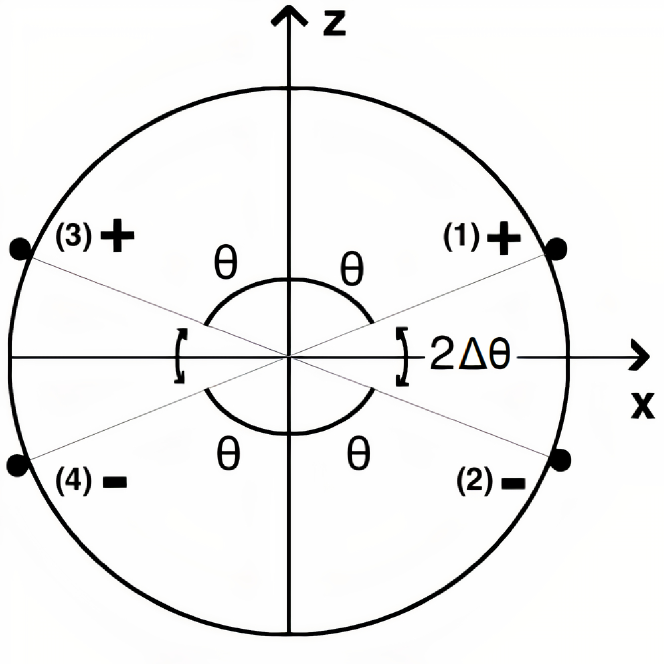
Figure 2: Coplanar symmetric configuration for four vortices numbered 1 to 4 and charged as shown. We choose initial azimuthal angles $\phi=0$ (vortices 1 and 2) and $\phi=\pi$ (vortices 3 and 4) and initial polar angles $\theta$ (vortices 1 and 3) and $\pi-\theta$ (vortices 2 and 4) measured from the $z$ axis. The figure shows the angular aperture $2\Delta\theta=\pi-2\theta$ for vortex dipoles (12) and (34), where $\Delta\theta=\pi/2-\theta$.

These four vortices behave intuitively in two simple limits: When the vortices are near the poles ($\theta\ll 1$), the two positive (negative) vortices circle the north (south) pole, acting like independent pairs of same-sign vortices, with a linear speed $\hbar/(2MR\theta)$, just like two same-sign vortices on a plane. Near the equator ($\theta\to\pi/2$ with $\Delta\theta=\pi/2-\theta\ll 1$) vortices ($1,2$) and ($3,4$) act like two independent vortex dipoles and move uniformly with speed $\hbar/(2MR\Delta\theta)$, straddling the equator. For intermediate configurations, all four vortices influence each other, requiring a more detailed analysis.

Use of Eq. (31) shows that

$$\dot{\bm{r}}_{k} = \sum_{j\neq k}\frac{\hbar}{4MR}\frac{q_{j}}{\sin^{2}(\gamma_{kj}/2)}\bigg{\{}-\left[\sin{\theta_{j}}\sin{(\phi_{k}-\phi_{j})}\right]\hat{\bm{\theta}}_{k}$$ (42)

$$+ \left[\sin\theta_{k}\cos\theta_{j}-\cos\theta_{k}\sin\theta_{j}\cos(\phi_{k}-\phi_{j})\right]\hat{\bm{\phi}}_{k}\bigg{\}}.$$

For each $k=1,\cdots,4$, a detailed analysis yields the simple result

$$\dot{\bm{r}}_{k}=\frac{\hbar}{MR}\frac{1}{\sin{2\theta}}\,\hat{\bm{\phi}}_{k}=\frac{\hbar}{MR}\frac{1}{\sin{2\Delta\theta}}\,\hat{\bm{\phi}}_{k},$$ (43)

where $\Delta\theta=\pi/2-\theta$. Since these four translational velocities are equal and in the positive azimuthal direction, the vortices all rotate together in a positive (counterclockwise) sense around $\hat{\bm{z}}$, remaining coplanar. In appropriate limits, Eq. (43) confirms our previous qualitative discussion.

V.1.2 exchanged (antisymmetric) configuration $+-+-$

Consider now a second coplanar case, the exchanged configuration, where we interchange the charge of the vortices 1 and 2 in Fig. 2, with $q_{1}=-1$ and $q_{2}=+1$, as shown in Fig. 3.

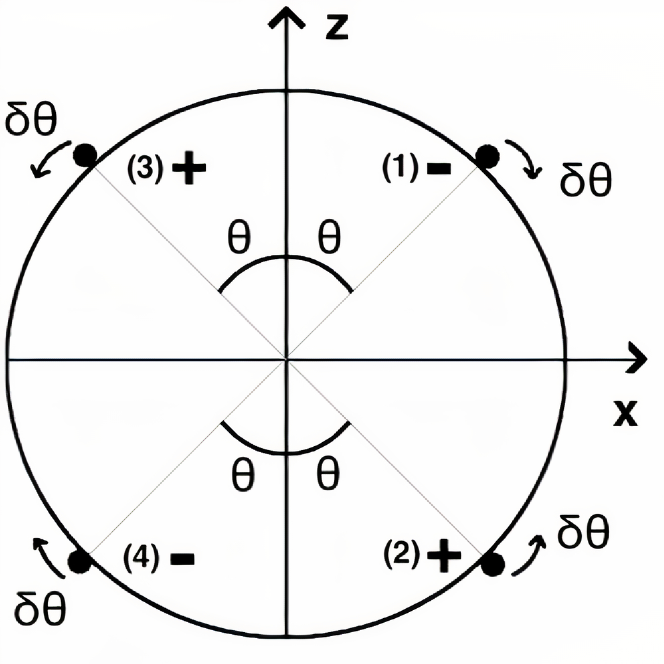
Figure 3: Coplanar exchanged (antisymmetric) configuration for $\theta=\pi/4$, including the small deviations $\delta\theta$ that provide the orbital motion around the equilibrium position.

For simplicity, we start with $\theta\ll 1$, when the motion is intuitively clear. Vortices (13) form a vortex dipole near the north pole, with vortices (24) similarly forming a vortex dipole near the south pole. Both dipoles move in the $yz$ plane at fixed $\phi=\pi/2$ toward the equator, where they interact and exchange partners. Vortices (12) then move westward as a dipole along the equator, while vortices (34) similarly move eastward, meeting on the opposite side of the sphere. They then exchange partners again and move toward the north (south) poles, respectively, where the cycle repeats. Note that the positive (negative) vortices execute a close path in the positive (negative) sense relative to the outward normal to the surface of the sphere (a video of the complete simulation is available in the Supplemental Material SM ). Alternatively, we could have started with $\Delta\theta\ll 1$ (see Fig. 2), which executes the same cycle with a different initial position. As discussed below Eq. (34), each vortex moves with speed $\hbar/(2MR\theta)$ and travels a distance $2\pi R$ in one complete cycle. Hence the period is $T=4\pi MR^{2}\theta/\hbar$ and the corresponding angular frequency is

$$\omega=\frac{2\pi}{T}=\frac{\hbar}{2MR^{2}\theta}.$$ (44)

The other simple initial configuration is $\theta=\pi/4$ (see Fig. 3). The sign exchange in the summed terms of Eq. (42) means that the velocities $\dot{\bm{r}}_{k}$ all vanish, yielding a static configuration of the four vortices. For small deviations of the initial positions with $\theta=\pi/4+\delta\theta$, numerical studies (see Supplemental Material SM ) show that each vortex executes a closed elliptical orbit around its equilibrium static configuration, with positive vortices moving in the positive sense and the negative ones in the negative sense, similar to the motion for the initial configuration $\theta\ll 1$. For $\delta\theta\ll 1$, the elliptical orbit has semiminor and semimajor axes $\approx R\,2\delta\theta$ and $\approx R\,4\delta\theta$ along $\hat{\bm{\theta}}$ and $\hat{\bm{\phi}}$ directions, respectively. Using the numerical data for various values of $\delta\theta$, we found that the analytical formula

$$\omega\approx\frac{\hbar}{MR^{2}}\frac{1}{\cos(2\delta\theta)}$$ (45)

provides a best fit to the numerical values of orbital frequency. For small $\delta\theta$, this frequency reduces to $\omega\approx\hbar/(MR^{2})$, whereas for small $\theta\ll 1$ and $\delta\theta\to-\pi/4$, Eq. (45) gives $\omega\approx\hbar/(2MR^{2}\theta)$, as expected for the orbital frequency of the dipoles in Eq. (44). The expression in Eq. (45) may well be exact, but we have not found a detailed proof.

For more general asymmetric $\theta$ configurations of the four vortices, they will rapidly lose their initial coplanar condition, and we are unable to predict their orbits analytically.

Finally we briefly discuss a three-dimensional tetrahedral configuration, with the vortices at four symmetric sites on the sphere. In contrast to four coplanar vortices, the tetrahedron has only one possible configuration: each positive site will have one positive neighbor and two negative neighbors, all at the same separations. Equation (42) shows that the tetrahedron is also a static vortex configuration. Unlike the planar configurations, however, it is an unstable equilibrium, with complicated dynamics even for small perturbations.

VI Energy and dynamics of two vortex dipoles

Section IV considered the energy of a general neutral system of vortices on the surface of a sphere, as given in Eq. (36). The next Sec. V then studied the dynamics of four vortices with zero net vortex charge in some simple symmetric configurations. Here, we examine the case of two small vortex dipoles, which is a different special configuration of four vortices with zero net vortex charge. For definiteness, we consider one dipole with charges $q_{1}=-q_{2}=1$ and another dipole with $q_{3}=-q_{4}=1$. Although Eq. (36) gives the total interaction energy of these two dipoles as a sum over six pairs of vortices, we instead provide a more physical picture.

As a first step, we focus on the dipole with vortices at angular positions $\Omega_{1}$ and $\Omega_{2}$ on the sphere. The total stream function is

$$\chi^{12}(\Omega)=\chi(\Omega,\Omega_{1})-\chi(\Omega,\Omega_{2}),$$ (46)

where Eq. (25) gives the stream function for each individual vortex. For the present case of a small vortex dipole centered at $\Omega_{0}$, we write $\delta\Omega_{0}=(\delta\theta_{0},\delta\phi_{0})=\Omega_{1}-\Omega_{2}$ and expand Eq. (46) to first order in the small angular separations. Define the vortex dipole moment (a vector)

$$\bm{p}_{0}=R\delta\theta_{0}\,\hat{\bm{\theta}}_{0}+R\sin\theta_{0}\,\delta\phi_{0}\,\hat{\bm{\phi}}_{0},$$ (47)

which has the dimension of a length, with $\hat{\bm{\theta}}_{0}$ and $\hat{\bm{\phi}}_{0}$ the unit spherical-polar vectors at $\Omega_{0}$ on the surface of the sphere. It is not difficult to find

$$\chi_{\rm dip}(\Omega)\approx-\frac{\bm{p}_{0}\cdot R(\hat{\bm{r}}-\hat{\bm{r}}_{0})}{R^{2}(\hat{\bm{r}}-\hat{\bm{r}}_{0})^{2}}=-\frac{\bm{p}_{0}\cdot({\bm{r}}-{\bm{r}}_{0})}{({\bm{r}}-{\bm{r}}_{0})^{2}},$$ (48)

where $\bm{r}=R\hat{\bm{r}}$ is the coordinate vector normal to the surface of the sphere and we note that $\bm{p}_{0}\cdot\hat{\bm{r}}_{0}=0$. This expression is completely analogous to the electrostatic potential arising from an electric dipole moment $\bm{p}$, here suitably modified for the two-dimensional character of a vortex dipole.

The interaction energy of this single vortex dipole follows directly from Eq. (36) and the subsequent discussion

$$E_{12}=\frac{2\hbar^{2}n\pi}{M}\chi_{12}=\frac{2\hbar^{2}n\pi}{M}\ln\left[2\sin\left(\frac{|\gamma_{12}|}{2}\right)\right].$$ (49)

For a small dipole with $|\gamma_{12}|\ll 1$, we find the simple expression

$$E_{12}\approx\frac{2\hbar^{2}n\pi}{M}\ln\left(|\gamma_{12}|\right)=-\frac{2\hbar^{2}n\pi}{M}\ln\left(\frac{R}{p_{12}}\right),$$ (50)

where $p_{12}=R|\gamma_{12}|$ is the separation between the two vortices (it is also the dipole moment). As a result, the energy of the two separate dipoles is

$$E_{\rm d}=\frac{2\hbar^{2}n\pi}{M}\left(\chi_{12}+\chi_{34}\right).$$ (51)

The interaction energy of the two dipoles is $E_{\rm dd}=Mn\int d^{2}r\,\bm{v}^{12}\cdot\bm{v}^{34}$, where $\bm{v}^{12}$ and $\bm{v}^{34}$ are the velocity fields of the two dipoles. Formally, we can use Eq. (46) and write

$$E_{\rm dd} = \frac{\hbar^{2}n}{M}\int d^{2}r\,\bm{\nabla}\chi^{34}\cdot\bm{\nabla}\chi^{12}$$ (52)

$$= \frac{\hbar^{2}n}{M}\int d^{2}r\,\bm{\nabla}(\chi_{3}-\chi_{4})\cdot\bm{\nabla}(\chi_{1}-\chi_{2})$$

$$= -\frac{2\pi\hbar^{2}n}{M}(\chi_{13}+\chi_{24}-\chi_{23}-\chi_{14}).$$

The sum of Eqs. (51) and (52) precisely reproduces the six terms inferred from Eq. (36).

More physically, we can find $\chi^{12}$ and $\chi^{34}$ directly from Eq. (48). In this way, the familiar integration by parts with the first line of Eq. (52) gives an explicit expression for the interaction energy of two small vortex dipoles $\bm{p}$ and $\bm{p}^{\prime}$ at positions $\bm{r}$ and $\bm{r}^{\prime}$:

$$E_{\rm dd}=\frac{2\pi\hbar^{2}n}{M}\,\frac{(\bm{p}\cdot\bm{p}^{\prime})\,(\bm{r}-\bm{r}^{\prime})^{2}-2\bm{p}\cdot(\bm{r}-\bm{r}^{\prime})\,\bm{p}^{\prime}\cdot(\bm{r}-\bm{r}^{\prime})}{(\bm{r}-\bm{r}^{\prime})^{4}}.$$ (53)

This rather complicated form is familiar from electrostatics and magnetostatics, suitably modified for the two dimensions relevant here. It varies inversely with the squared separation of the dipoles and is highly anisotropic through the dependence on each dipole’s orientation.

We emphasize that Eq. (53) only applies for large separations $|\bm{r}-\bm{r}^{\prime}|^{2}\gg pp^{\prime}$ and does not hold for two nearby dipoles. In such a case, we must rely on the general expression from Eq. (36), involving a sum over all six distinct pairs of vortices.

It is interesting to consider the dynamics of two small vortex dipoles on a sphere, say $\bm{p}_{i}$ and $\bm{p}_{i}^{\prime}$. When the two dipoles are well separated, the total energy is the sum of their individual dipole energies $E_{\rm tot}=-(\pi\hbar^{2}n/M)\ln(R^{2}/p_{i}p_{i}^{\prime})$, and the magnitudes $p_{i}$ and $p_{i}^{\prime}$ remain fixed as each moves along a great circle at speed $\hbar/Mp_{i}$ and $\hbar/Mp_{i}^{\prime}$, respectively

If they approach each other, the dynamics becomes complicated, requiring a detailed analysis. Nevertheless, some general conclusions are possible. For two small nearby dipoles, they interact locally on the tangent plane. We can then invoke the conservation law from Eq. (18), which now implies that the total dipole moment is conserved along with the total energy. In an obvious notation for initial and final dipole moments, we have $\bm{p}_{i}+\bm{p}_{i}^{\prime}=\bm{p}_{f}+\bm{p}_{f}^{\prime}$ and the conservation of energy implies that $p_{i}p_{i}^{\prime}=p_{f}p_{f}^{\prime}$.

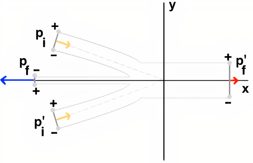
Figure 4: Two vortex dipoles $\bm{p}_{i}$ and $\bm{p}_{i}^{\prime}$ move to the right on nearly parallel converging trajectories. Once they are sufficiently close, the individual vortices rearrange to form two new vortex dipoles, with $\bm{p}_{f}$ moving rapidly to the left and $\bm{p}_{f}^{\prime}$ moving slowly to the right. The solid lines show calculated orbits for the initial conditions.

We already discussed a specific example of two dipoles on a sphere in connection with Fig. 3, when one dipole starts at the north pole and the other starts at the south pole as shown for small dipoles with $\theta\ll 1$. Here we assume that $p_{i}^{\prime}=p_{i}=2R\theta$. After the interaction, the reconstructed dipoles move around the equator in opposite directions, and the conservation laws then show that $p_{f}=p_{f}^{\prime}=2R\theta$ during this part of their orbits.

A more unusual situation arises for two nearly parallel dipoles that gradually approach each other (see Fig. 4) in the tangent plane, labeled by axes $x$ and $y$. Here the initial dipole moments are $\bm{p}_{i}\approx\bm{p}_{i}^{\prime}\approx p\hat{\bm{y}}$, and their motion is principally along $\hat{\bm{x}}$ (converging slowly toward the $x$ axis), with each having a small velocity component along $\hat{\bm{y}}$. After the interaction, the two inner vortices form a new smaller dipole $\bm{p}_{f}=-p_{f}\hat{\bm{y}}$ that moves to the left. In contrast, the two outer vortices form a new larger dipole $\bm{p}_{f}^{\prime}=p_{f}^{\prime}\hat{\bm{y}}$ that continues moving to the right. The conservation of dipole moment requires $2p=p_{f}^{\prime}-p_{f}$, and the conservation of energy shows that $p^{2}=p_{f}p_{f}^{\prime}$. Simple algebra yields the final values $p_{f}^{\prime}/p=\sqrt{2}+1$ and $p_{f}/p=\sqrt{2}-1$. As a result, we have a very asymmetric configuration with $p_{f}^{\prime}/p_{f}=3+2\sqrt{2}\approx 5.83$. These two new dipoles move in opposite directions around a single great circle at different speeds, with $v_{f}/v_{f}^{\prime}=3+2\sqrt{2}\approx 5.83$, but they eventually meet. After interacting a second time, they separate and move on nearby great circles toward their initial configuration (see Supplemental Material SM for a video of the early evolution of two colliding dipoles).

VII Summary and Conclusions

We presented the dynamics and stability of singly charged vortices in a thin spherical “bubble” BEC. The topology of this system constrains the configuration of vortices to an even number of vortices with total charge zero. We calculated the velocity fields and energies of various configurations of vortices and dipoles, which allow us to determine their dynamics on the surface of the sphere. In some cases, two initial small vortex dipoles can interact and exchange partners. The final reconfigured dipoles then separate and follow new trajectories.

Proposed new experiments in microgravity conditions Aveline et al. (2020) means that our model of a thin “bubble” trapped BEC may be studied experimentally in the near future. In addition, recent experiments have studied a “bubble” trap potential in the presence of gravity De Rossi et al. (2016); Guo et al. (2020), and it may soon be feasible to manipulate the trap rotation and the atomic parameters to fix various initial conditions. We anticipate that our theoretical studies will be relevant for any further studies on the evolution of vortex pairs on a sphere. We plan to provide theoretical explanations for these experimental results, adapting our model to include the effect of the gravitational potential Sun et al. (2018).

VIII Acknowledgments

We are grateful to Pietro Massignan for helpful discussions. This work was supported by the São Paulo Research Foundation (FAPESP) under Grant No. 2013/07276-1. The authors also thank Coordenação de Aperfeiçoamento de Pessoal de Nível Superior (CAPES) for their financial support.

Supplemental Material: Superfluid vortex dynamics on a spherical film

See https://youtu.be/QqWxwSvG2o8 for a video displaying a complete simulation of the dynamics of two vortex-dipoles. We start with $\theta\ll 1$ (see Fig. 3 in the main text). The vortex pair black (positively charged) - red (negatively charged) forms a vortex dipole near the north pole. Similarly, the blue (positive) - orange (negative) vortices form a vortex dipole near the south pole. Both dipoles move in the $yz$ plane toward the equator, where they interact and exchange partners. The new dipoles then move along the equator, meeting on the opposite side of the sphere. They then exchange partners again, with one of the new dipoles moving toward the north pole and the other towards the south pole, restarting the cycle.
Moreover, see https://youtu.be/U2b2oKtFjMA for a video displaying a simulation of the vortices’ orbits for small deviations of their initial positions with $\theta=\pi/4+\delta\theta$ (see Fig. 3). Each vortex executes a closed elliptical orbit around its equilibrium static configuration, with positive vortices (black and blue) moving in the positive sense and the negative ones (red and orange) in the negative sense, similar to the motion for the initial configuration $\theta\ll 1$.

See https://youtu.be/GP6VTKZOm7A for a video of the collision of two asymmetric dipoles (different speeds) with parameters set as in Fig. 4 of the main text. Initially, the slow pair $``$black (positively charged) - red (negatively charged)$"$ form a vortex dipole near the north pole, with the fast pair $``$blue (positive) - orange (negative)$"$ forming a vortex dipole near the south pole. After the interaction, the two initial dipoles exchange their components and form two equal-size (same speed) dipoles which move slightly tipped great circles that intersect on the opposite side of the sphere. Then they swap pairs again and reconstruct the initial dipoles configuration. This process repeats cyclically.

The unit of length in these simulations is the radius of the sphere $R$ and the unit of time is $MR^{2}/\hbar$, with $M$ being the atomic mass.

References

- Pethick and Smith (2008) C. Pethick and H. Smith, Bose-Einstein condensation in Dilute Gases, 2nd ed. (Cambridge University Press, New York, 2008).
- Pitaevskii and Stringari (2016) L.P. Pitaevskii and S. Stringari, Bose-Einstein Condensation and Superfluidity, 2nd ed. (Oxford University Press, New York, 2016).
- Bloch et al. (2008) I. Bloch, J. Dalibard, and W. Zwerger, “Many-body physics with ultracold gases,” Rev. Mod. Phys. 80, 885–964 (2008).
- Elliott et al. (2018) E.R. Elliott, M.C. Krutzik, J.R. Williams, R.J. Thompson, and D.C. Aveline, “Nasa′s cold atom lab (cal): system development and ground test status,” npj Microgravity 4, 1–7 (2018).
- Lundblad et al. (2019) N. Lundblad, R.A. Carollo, C. Lannert, M.J. Gold, X. Jiang, D. Paseltiner, N. Sergay, and D.C. Aveline, “Shell potentials for microgravity Bose-Einstein condensates,” npj Microgravity 30, 1–6 (2019).
- Bereta et al. (2019) S.J. Bereta, L. Madeira, V.S. Bagnato, and M.A. Caracanhas, “Bose-Einstein condensation in spherically symmetric traps,” American Journal of Physics 87, 924 (2019).
- Tononi and Salasnich (2019) A. Tononi and L. Salasnich, “Bose-Einstein condensation on the surface of a sphere,” Phys. Rev. Lett. 123, 160403 (2019).
- Guenther et al. (2017) N. Guenther, P. Massignan, and A.L. Fetter, “Quantized superfluid vortex dynamics on cylindrical surfaces and planar annuli,” Phys, Rev. A 96, 063608 (2017).
- Massignan and Fetter (2019) P. Massignan and A.L. Fetter, “Superfluid vortex dynamics on planar sectors and cones,” Phys. Rev. A 99, 063602 (2019).
- Turner et al. (2010) A.M. Turner, V. Vitelli, and D.R. Nelson, “Vortices on curved surfaces,” Rev. Mod. Phys. 82, 1301–1348 (2010).
- Lamb (1945) H. Lamb, Hydrodynamics, 6th ed. (Dover Publications, New York, 1945).
- Butkov (1973) E. Butkov, Mathematical Physics (Addison-Wesley, 1973).
- (13) See Supplemental Material at [URL will be inserted by publisher] for complete simulations of (i) of the dynamics of two vortex-dipoles; (ii) for a video displaying a simulation of the vortices’ orbits for small deviations of their initial positions; and (iii) for a video of the collision of two asymmetric dipoles (different speeds) with parameters set as in Fig. 4 of the main text .
- Aveline et al. (2020) D.C. Aveline, J.R. Williams, E.R Elliott, C. Dutenhoffer, J.R. Kellogg, J.M. Kohel, N.E. Lay, K. Oudrhiri, R.F. Shotwell, N. Yu, and R.J. Thompson, “Observation of Bose-Einstein condensates in an earth orbiting research lab,” Nature 582, 193–197 (2020).
- De Rossi et al. (2016) C. De Rossi, R. Dubessy, K. Merloti, M.G. de Herve, T. Badr, A. Perrin, L. Longchambon, and H. Perrin, “Probing superfluidity in a quasi two-dimensional Bose gas through its local dynamics,” New Journal of Physics 18, 062001 (2016).
- Guo et al. (2020) Y. Guo, R. Dubessy, M.G. de Herve, A. Kumar, T. Badr, A. Perrin, L. Longchambon, and H. Perrin, “Supersonic rotation of a superfluid: A long-lived dynamical ring,” Phys. Rev. Lett. 124, 025301 (2020).
- Sun et al. (2018) K. Sun, K. Padavić, F. Yang, S. Vishveshwara, and C. Lannert, “Static and dynamic properties of shell-shaped condensates,” Phys. Rev. A 98, 013609 (2018).