Unruh effect and information entropy approach

Abstract

Total entropy generated by the Unruh effect is calculated within the framework of information theory. In contrast to previous studies, here the calculations are done for the finite time of existence of the non-inertial reference frame. In this case only the finite number of particles is produced. Dependence on mass of the emitted particles is taken into account. Analytic expression for the entropy of radiated boson and fermion spectra is derived. We study also its asymptotics corresponding to limiting cases of low and high acceleration. The obtained results can be further generalized to other intrinsic degrees of freedom of the emitted particles, such as spin and electric charge.

I Introduction

As was demonstrated by Unruh [1], the observer comoving with non-inertial reference frame (RF) with acceleration $a$ will detect particles thermalized at temperature

$$T=\frac{a}{2\pi}$$

in Planck units, whereas the observer in any inertial RF will see bare vacuum. If acceleration $a$ equals to surface gravity of some Schwarzschild black hole (BH), then $T$ coincides with the temperature $T_{\mathrm{BH}}$ of Bekenstein-Hawking radiation [2, 3] of the horizon.

This peculiar non-invariance of vacuum has raised a lot of interest to the topic, for review see, e.g., [4] and references therein. Recall that the Unruh effect initially was derived for scalar particles. Here the change in the ratio between negative and positive frequency modes of scalar fields in the noninertial RF was considered [1]. Generalizations to arbitrary trajectories of the observer is discussed in [5], whereas the generalization to accelerated reference frames with rotation can be found in [6]. The emergence of the Unruh effect in Rindler manifold of arbitrary dimension and its relationship to the vacuum noise and stress are investigated in [7]. Various methods and approaches have been employed. For instance, algebraic approach was used to extend the Unruh effect to theories with arbitrary spin and with interaction [8], whereas the path integral approach was applied to derive the effect for fermions within the framework of quantum field theory [9]. Among the recent studies one can mention the relativistic quantum statistical mechanics approach [10, 11, 12] based on application of Zubarev’s density operator [13, 14]. Within this approach the Unruh effect was obtained first for scalar particles [10] and then generalized to the gas of massless fermions [12]. In the present study we employ the approach based on application of the information theory which was not elaborated extensively yet.

Usually the non-inertial observer is assumed to accelerate forever. However, such an assumption implies availability of infinite energy supply and ever-lasting particle emission. The more sophisticated scenario which considers the Unruh effect at finite time interval is analyzed in [15, 16].

There is a lot of proposals for the detection and application of the Unruh effect, see, e.g., [17, 18, 19]. Paper [20] discusses possibility of eavesdropping in the non-inertial reference frame. Production of the entangled photon pairs from the vacuum with the help of the Unruh effect was investigated in [21], whereas in [22] creation of accelerated black holes by means of the Unruh effect was studied. In [23] the authors discuss possibility of using accelerated electrons as thermometers. Generated bosons and fermions were considered as being produced via the quantum tunneling mechanism at the Unruh horizon in [24, 25].

The Unruh effect may be considered as a source of particle production. The idea has been widely employed [26, 27, 28, 29, 30, 31, 32, 33] in order to explain multiparticle production in hadronic and heavy-ion collisions at ultrarelativistic energies. The attractive feature of application of the Unruh effect as possible mechanism of the multiparticle production is the thermalized spectra of newly produced particles. Experiments with ultrarelativistic hadronic and heavy-ion collisions and their theoretical interpretations indicate that the produced matter seems to reach equilibrium extremely quickly, see, e.g., [34, 35] for present status of the field. The mechanism of this fast equilibration is still debated, therefore, the Unruh effect might be of a great help. At the same time, since the Unruh source is thermal, it results in observer-dependent entropy generation [36]. In the present paper we also consider the Unruh horizon as a thermal source of particles. These particles are characterized by thermal distribution. Our aim is to estimate the entropy of the distribution and to define its dependence on any intrinsic degrees of freedom of the emitted particles.

The paper is organized as follows. Section II presents the necessary basics from probability theory and information theory. Section III briefly describes Unruh effect and density matrix of the emitted quanta. The total entropy of the Unruh source is estimated in Sect. IV. Here the general expression for the entropy of fermion and boson radiation is derived, as well as its analytic series expansion. In Sect. V one is dealing with the analysis of temperature asymptotics of the entropy. Two limiting cases corresponding to low and high temperature, or, equivalently, acceleration of the observer, are considered. Section VI is devoted to contribution of intrinsic degrees of freedom of the produced particles. Final remarks and conclusions can be found in Sect. VII.

II Probability and entropy

Let us consider some distribution $\{X\}$ with unnormalized distribution probability $d\left(x\right)$. In other words, $d\left(x\right)$ is a number of events in which $x$ has being observed. Shannon entropy $H\left(X\right)$ for it may be written as

$$\begin{split}H\left(X\right)&=-\sum_{x}\frac{d\left(x\right)}{\mathcal{D}_{X}}\ln\frac{d\left(x\right)}{\mathcal{D}_{X}}\\ &=\ln\mathcal{D}_{X}-\frac{1}{\mathcal{D}_{X}}\sum_{x}d\left(x\right)\ln d\left(x\right)\ ,\end{split}$$ (1)

where $\mathcal{D}_{X}=\sum_{x}d\left(x\right)$. $H\left(X\right)$ encodes amount of information we need in order to completely describe $\{X\}$, i.e., this is amount of information we are lacking. Therefore, we should deal with the distribution $\{X\}$. It is scale-invariant, so it does not changed under the transformations $d\left(x\right)\to\alpha d\left(x\right)$ for any $\alpha=const$.

Similarly, for joint distribution $\{X,Y\}$ with unnormalized distribution probability $d\left(x,y\right)$ one can write down Shannon entropy $H\left(X,Y\right)$ as

$$\begin{split}H\left(X,Y\right)&=-\sum_{x,y}\frac{d\left(x,y\right)}{\mathcal{D}_{X,Y}}\ln\frac{d\left(x,y\right)}{\mathcal{D}_{X,Y}}\\ &=\ln\mathcal{D}_{X,Y}-\frac{1}{\mathcal{D}_{X,Y}}\sum_{x,y}d\left(x,y\right)\ln d\left(x,y\right),\end{split}$$ (2)

where $\mathcal{D}_{X,Y}=\sum_{x,y}d\left(x,y\right)$.

In the joint case one may define conditional probability $d\left(x|y\right)$ as

$$d\left(x|y\right)=\frac{d\left(x,y\right)}{d\left(y\right)}\ ,\qquad d\left(y\right)=\sum_{x}d\left(x,y\right).$$ (3)

It defines the amount of events with $x$ from the set of events in which $y$ occurs. Using Eq. (1), Shannon entropy $H\left(X|y\right)$ becomes

$$\begin{split}H\left(X|y\right)&=\ln\mathcal{D}_{X|y}-\frac{1}{\mathcal{D}_{X|y}}\sum_{x}d\left(x|y\right)\ln d\left(x|y\right)\\ &=-\sum_{x}d\left(x|y\right)\ln d\left(x|y\right),\end{split}$$ (4)

where $\mathcal{D}_{X|y}=\sum_{x}d\left(x|y\right)=1$, as follows from Eq. (3).

Finally, substituting Eq. (3) and Eq. (4) into Eq. (2) one gets

$$\begin{split}H\left(X,Y\right)&=H\left(Y\right)+\Braket{H\left(X}{y}_{Y}\\ &=H\left(X\right)+\Braket{H\left(Y}{x}_{X},\end{split}$$ (5)

where averaging taken over ${X}$ or ${Y}$ reads

$$\Braket{\mathcal{A}}_{Z}=\frac{1}{\mathcal{D}_{Z}}\sum_{z}d\left(z\right)\mathcal{A}\ ,\qquad Z\equiv X,Y.$$

Recall, that all the formulae above are valid for discrete distributions only. In the continuous case one should use probability density function (PDF) $p\left(x\right)$ instead of $d\left(x\right)$. Shannon entropy becomes dimensional incorrect then and should be re-defined, as shown in [37, 38].

For distribution $\{X\}$ with PDF $p\left(x\right)$ the entropy given by Eq. (1) is generalized to

$$H\left(X_{p}\right)=\ln\mathcal{D}_{X_{p}}-\frac{1}{\mathcal{D}_{X_{p}}}\int p\left(x\right)\ln p\left(x\right){\rm d}x-\Braket{\ln{\rm d}x}_{X_{p}},$$ (6)

where $\mathcal{D}_{X_{p}}=\int p\left(x\right){\rm d}x$ is the norm and

$$\Braket{\mathcal{A}}_{X_{p}}=\frac{1}{\mathcal{D}_{X_{p}}}\int p\left(x\right)\mathcal{A}{\rm d}x.$$

The last term in Eq. (6) is related to the limiting density of discrete points and takes into account amount of information encoding discrete-continuum transition, see [37, 38] for details. Note, that one may formally reduce $H\left(X_{p}\right)$ to $H\left(X\right)$ by substituting $\int p\left(x\right){\rm d}x$ into $\sum_{x}d\left(x\right)$ and setting $\left\langle\ln{\rm d}x\right\rangle_{X_{p}}$ to zero; the same procedure is valid also in the opposite direction.

III Unruh effect

From here we will use Planck (or natural) units, $c=G=\hbar=k_{B}=1$. Also, we restrict our analysis to $1+1$-dimensional space-time, because two other spatial dimensions play no role and, therefore, can be neglected.

As was already mentioned in Sec. I, vacuum is non-invariant with respect to the reference frame [1]. In the non-inertial RF determined with the acceleration $a$ one meets with the appearance of horizon separating space-time to the inside and outside domains. As a result, the non-inertial observer detects radiation going out from the horizon, while the inertial one detects the vacuum state $|0\rangle$ only. For bosons the latter reads [4, 24, 25]

$$\Ket{0}=\sqrt{\frac{1-\exp{\left(-E/T\right)}}{1-\exp{\left(-NE/T\right)}}}\sum_{n=0}^{N-1}\exp{\left(-nE/2T\right)}\Ket{n}_{\rm in}\Ket{n}_{\rm out}\ ,$$ (7)

whereas for fermions one gets

$$\Ket{0}=\frac{1}{\sqrt{1+\exp{\left(-E/T\right)}}}\sum_{n=0}^{1}\exp{\left(-nE/2T\right)}\Ket{n}_{\rm in}\Ket{n}_{\rm out}$$ (8)

Here $E$ is the energy of the quanta emitted at Unruh horizon with temperature $T=a/\left(2\pi\right)$. Parameter $N$, as can be seen from Eq. (7), encodes maximum amount of quanta at energy $E$ plus 1. Loosely speaking $N$ is a number of dimensions of the corresponding Fock space at given energy $E$ and temperature $T$ of the source. The subscripts in and out denote the components of the field with respect to the horizon.

Usually $N$ is assumed to be infinite. But taking $N\to\infty$ in Eq. (7), as it is widely used in the literature on the topic, seems to be too strong assumption, because the source is considered to produce infinite amount of energy, $\left(N-1\right)E\to\infty$. This is valid in case of everlasting acceleration that can be provided with the infinite energy supply only. Such a case seems to be rather unlikely, therefore we assume maximum number of particles to be finite in all the calculations below. Also, let us consider only boson production in what follows, because the expression for fermions given by Eq. (8) can be derived from Eq. (7) by setting $N=2$.

Expression (7) is Schmidt decomposition [39]. The outgoing radiation is described by density matrix

$$\begin{split}\rho_{\rm out}&={\rm Tr}_{\rm in}\Ket{0}\Bra{0}\\ &=\frac{1-\exp{\left(-E/T\right)}}{1-\exp{\left(-NE/T\right)}}\sum_{n=0}^{N-1}\exp{\left(-\frac{nE}{T}\right)}\Ket{n}_{\rm out}\Bra{n}_{\rm out}\ ,\end{split}$$ (9)

where we have traced over the inaccessible degrees of freedom (in- modes). Thus, pure vacuum state from the inertial RF has transformed into the mixed one in the non-inertial RF. Here appears the geometric origin of the Unruh effect. Namely, finiteness of the speed of light leads to appearance of the horizon dividing the all modes in Hilbert space into the accessible (out-) and non-accessible (in-) ones. The complete state is obviously pure and follows unitary evolution. But because one has limited access to it in the non-inertial RF, it looks like a decoherence. Eigenvalues of density matrix $\rho_{\rm out}$ define emission probability of certain number of particles at energy $E$ and temperature $T$. Therefore, Eq. (9) describes conditional multiplicity distribution $\{n|N,E,T\}$ at given $N,\ E$ and $T$.

IV Unruh entropy

For the emission probability $\rho_{\rm out}$ from Eq. (9) the von Neumann entropy is defined as

$$\begin{split}H\left(\rho_{\rm out}\right)&=-{\rm Tr}\rho_{\rm out}\ln\rho_{\rm out}=H\left(n|N,E,T\right)\\ &=\sigma\left(qE/T\right)\Big{|}_{q=N}^{q=1}\ ,\end{split}$$ (10)

where we use the following notations

$$\sigma\left(qE/T\right)=\frac{qE/T}{\exp{\left(qE/T\right)}-1}-\ln{\left[1-\exp{\left(-\frac{qE}{T}\right)}\right]}\ ,$$ (11)

$$f\left(x\right)\Big{|}^{x=a}_{x=b}=f\left(a\right)-f\left(b\right)\ .$$ (12)

As one may notice, $H\left(n|N,E/T\right)$ is an even function of $E/T$, i.e. $H\left(n|N,E/T\right)=H\left(n|N,-E/T\right)$. Asymptotic behavior of entropy (10) with respect to $E/T$ is the following

$$\begin{split}\lim_{E/T\to 0}H\left(n|N,E,T\right)&=\ln N=\max\left(H\right)\\ \lim_{E/T\to\infty}H\left(n|N,E,T\right)&=0\ .\end{split}$$ (13)

Expression (10) defines entropy of the emitted quanta, as well as the quanta inside the horizon, for some mode of the radiated field only, which is determined by parameter $N$, energy $E$ and temperature $T$. Parameter $N$ depends on amount of time during which the observer is being described by non-inertial reference frame. It follows from the fact that the longer one is observing the horizon, the more particles at any fixed energy may be detected. Therefore we conclude that $N$ should increase with time. Temperature $T$ is completely determined by the acceleration $a$, see [1]. However, $E$ cannot be considered as a fixed parameter. The non-inertial observer is expected to detect particles at different energies. Energy range for the particles may be written as

$$m\leq E\leq M\ ,$$

where $m$ is invariant mass of the particles, and $M$ is the maximum energy to be observed, respectively. We assume $M$ to be limited by acceleration $a$, since observation of the high energy particles is very unlikely due to energy conservation law: one cannot extract more energy from the vacuum than is being spent to sustain the observer’s acceleration.

Unfortunately, definition of the energy range does not mean we know the spectrum distribution $\{E\}$. It is determined by unnormalized PDF $p\left(E\right)$ of emission of a particle from vacuum at energy $E$.

In order to figure out $p\left(E\right)$ somehow we use the following procedure. As can be noticed from Eq. (9), for any particle number $n>0$ the emission probability is proportional to factor $\exp{(-E/T)}$. Case with $n=0$ means no emission at all. Therefore, one should expect exponential behavior for $p\left(E\right)$

$$p\left(E\right)=C\exp{\left(-E/T\right)}\ ,$$ (14)

where prefactor $C$ is responsible for any corrections that might depend on the particle type and its quantum numbers. For the sake of simplicity we assume $C={\rm const}$ and, therefore, drop it due to normalization reasons, see Sect. II, in what follows. It is worth noting that such assumption results in Schwinger-like mechanism of particle production [40]. Thus we recovered Schwinger-like particle production from the properties of Hilbert space and space-time only. Recall, however, that this result is generated by Unruh effect after neglecting all the possible corrections.

Now we have spectrum distribution $\{E\}$ as given by Eq. (14). Without any loss of generality we assume energy to be defined within the range $m\leq E\leq M$. From Eq. (5) and Eq. (6) one gets

$$H\left(n,E|N,T\right)=-\Braket{\ln{\rm d}E}_{E_{p}}+\ln\mathcal{D}_{E_{p}}-\frac{1}{\mathcal{D}_{E_{p}}}\int_{m}^{M}p\left(E\right)\ln p\left(E\right){\rm d}E+\frac{1}{\mathcal{D}_{E_{p}}}\int_{m}^{M}p\left(E\right)H\left(n|N,E,T\right){\rm d}E.$$ (15)

In order to get analytic expression, we substitute Eq. (14) and Eq. (10) into Eq. (15) and obtain after the straightforward calculations total Unruh entropy $H\left(n,E|N,T\right)$ in a form

$$\begin{split}H\left(n,E|N,T\right)=&-\Braket{\ln{\rm d}E}_{E_{p}}+1+\ln\mathcal{D}_{E_{p}}+\frac{m\exp{\left(-m/T\right)}-M\exp{\left(-M/T\right)}}{\mathcal{D}_{E_{p}}}\\ &+\frac{T}{\mathcal{D}_{E_{p}}}\sum_{k=1}^{\infty}\Bigg{\{}\left[\frac{2kq+1}{k\left(kq+1\right)}+q\frac{E}{T}\right]\times\frac{\exp{\left[-(kq+1)E/T\right]}}{kq+1}\bigg{|}_{E=M}^{E=m}\Bigg{\}}\Bigg{|}_{q=N}^{q=1}\ ,\end{split}$$ (16)

where

$$\mathcal{D}_{E_{p}}=\int_{m}^{M}p\left(E\right){\rm d}E=T\left[\exp{\left(-\frac{m}{T}\right)}-\exp{\left(-\frac{M}{T}\right)}\right]$$ (17)

and $\sigma\left(qE/T\right)$ from Eq. (10) is represented by the following series

$$\sigma(qE/T)=\sum_{k=1}^{\infty}\left(\frac{1}{k}+q\frac{E}{T}\right)\exp{\left(-\frac{kqE}{T}\right)}.$$ (18)

The first term in Eq. (16) is responsible for encoding discrete-continuum transition, see [37, 38]. It is expected to depend neither on any quantum numbers of outgoing particles nor on the reference frame. Therefore, we assume $\Braket{\ln{\rm d}E}_{E_{p}}$ to be constant.

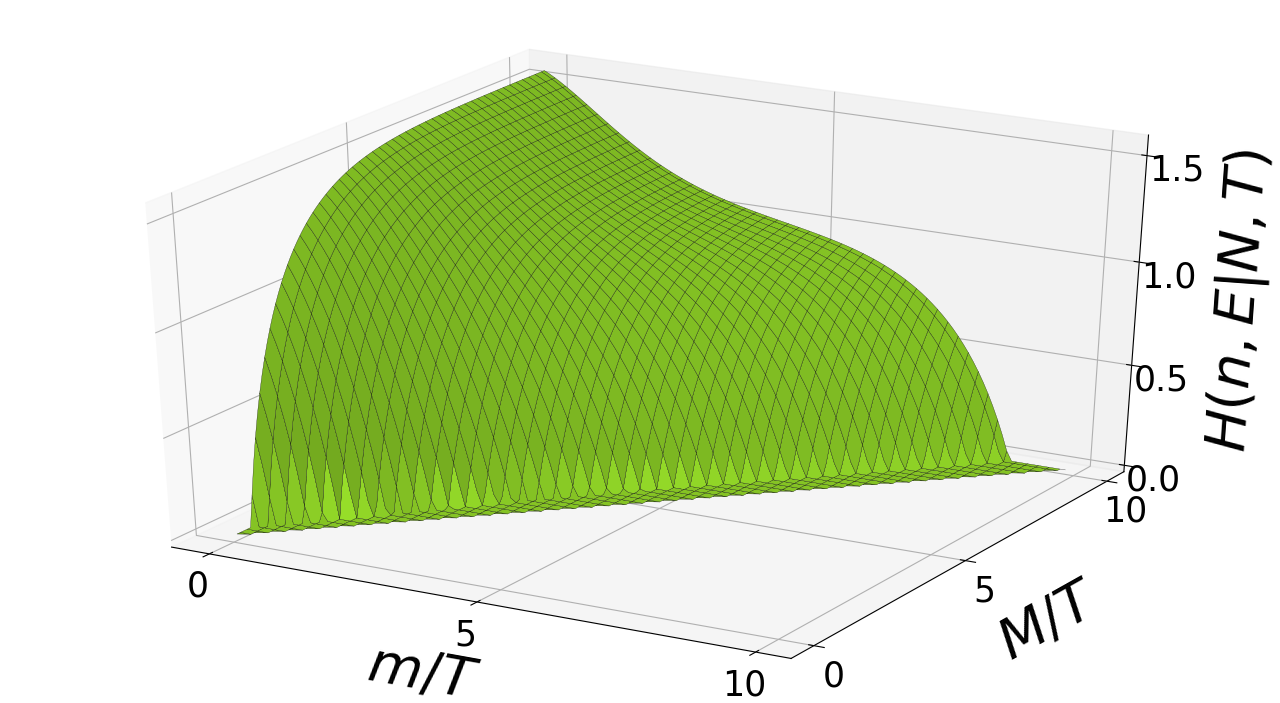
Figure 1: (Color online) Entropy $H(n,E|N,T)$ of Unruh radiation given by Eq. (16) for fermions $(N=2)$ as function of $m/T$ and $M/T$.

Expression (16) defines entropy for the distribution $\{n,E|N,T\}$ of the particles being detected by the observer associated to non-inertial RF moving with acceleration $a=2\pi T$. Recall, that in case of fermions one should use $N=2$. For bosons $N$ may take any positive integer value obeying the energy conservation law. The entropy calculated for the Unruh radiation of fermions and bosons is presented in Fig. 1 and Fig. 2, respectively. One can see the distinct maximum in the region of small values of $m/T$ ratio. The maximum increases with rising $M/T$ ratio and becomes more pronounced with the increase of radiated particles, see Fig. 2.

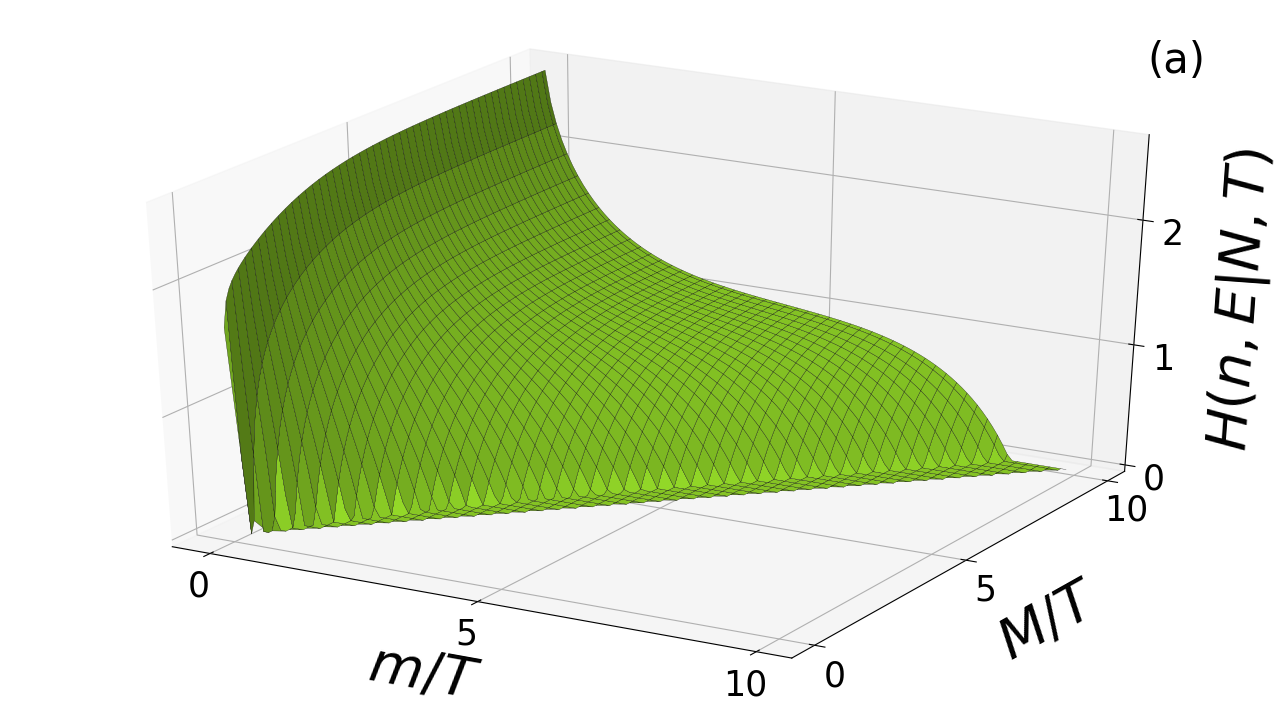
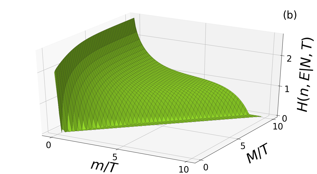
Figure 2: (Color online) The same as Fig. 1 but for bosons. The spectrum of bosons contains (a) $N=100$ and (b) $N=1000$ particles.

The considered example seems to be straightforward. However, one should keep in mind that all the analysis above is valid for $1+1$-dimensional space-time. Other spatial dimensions do not contribute to the density matrix $\rho_{\rm out}$ or to its von Neumann entropy, because the corresponding subspaces of the Hilbert space contribute to $\rho_{\rm out}$ via direct tensor product and, therefore, can be traced out with no consequences to the analysis above. This simple direct extension to additional spatial dimensions for Unruh effect may lead to widely-spread conclusion that Unruh effect results in appearance of thermal bath all over the space. In our opinion this conclusion needs to be clarified. Namely, in the last case the non-inertial observer, as well as the horizon itself, should be considered as an infinite plane in the additional spatial dimensions being accelerated alongside the normal to the plane. But the observer should be finite and, therefore, cannot detect particles from the half-space defined by the horizon. Otherwise, it would lead to faster-than-light speed communication and to causality violation, because the transition to inertial RF cannot cause immediate disappearance of the Unruh radiation from the horizon occupying the half-space.

To overcome the difficulties we have to assume that

• In order to obey energy conservation law $N$ should be finite.

• In case of (2+1) or (3+1)-dimensional space-time the Unruh horizon should be considered as radiation source of finite size.

Due to axial symmetry of the non-inertial reference frame the horizon should be of disk shape with some radius $r$. The radius can be determined by the observer’s size and causality, i.e. finiteness of light speed. Such an assumption leads to observer-dependent size of $r$. The problem may be cured, e.g., if one considers the observer’s acceleration $a$ as a surface gravity of the corresponding black hole and obtain some efficient scale $r=\left(4\pi T\right)^{-1}$.

One might be confused by the fact that since the Unruh effect describes the thermal bath its entropy should be maximal. As can be easily noticed from the eigenvalues of the density matrix (9), all of them exponentially depend on the total energy of the emitted number of particles and thus generate a well-known partition function. Note, however, that $\rho_{\rm out}$ is defined for some fixed value of energy. Therefore, $E$ can be considered as a parameter of the conditional distribution $\left\{n|N,E,T\right\}$. Dealing with joint distribution $\left\{n,E|N,T\right\}$ over multiplicity $n$ and energy $E$ of the emitted quanta one should take into account energy conservation. It results in some correlations between the possible number of emitted particles and their energy. Thus, the entropy $H\left(n,E|N,T\right)$ describes not a completely thermal source but some other one.

V Asymptotics of Unruh entropy

Let us analyze asymptotic behavior of total Unruh entropy (15) for (i) small and (ii) large acceleration of the observer. The case of small acceleration is analogous to $T\to 0$, therefore, we will drop all but the leading term in Eq. (15). At small temperatures Eq. (17) transforms to

$$\mathcal{D}_{E_{p}}\Big{|}_{T\to 0}\approx T\exp{\left(-m/T\right)},$$ (19)

where we have neglected the term $\exp{(-M/T)}$ since $M$ is the upper bound for the energy spectrum and, therefore, $M>m$. The Unruh entropy becomes

$$\begin{split}H\left(E\right)\Big{|}_{T\to 0}&=\ln\mathcal{D}_{E_{p}}-\frac{1}{\mathcal{D}_{E_{p}}}\int_{m}^{M}p\left(E\right)\ln p\left(E\right){\rm d}E\\ &\approx\ln T-\frac{m}{T}+1+\frac{m}{T}=\ln T+1.\end{split}$$ (20)

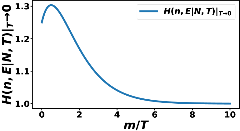
Figure 3: (Color online) Asymptotic behavior of entropy $H(n,E|N,T)$ given by Eq. (22) at $T\rightarrow 0$ as function of $m/T$.

Because the entropy $H\left(n|N,E,T\right)$ equals to zero when $N=1$, we consider the case with $N>1$ for $T\to 0$. Neglecting all higher order exponents, one obtains from Eq. (10) that

$$H\left(n|N,E,T\right)\Big{|}_{T\to 0}\approx\frac{E}{T}\exp{\left(-E/T\right)}.$$ (21)

Substituting Eq. (20) and Eq. (21) into Eq. (15) we get

$$H\left(n,E|N,T\right)\Big{|}_{T\to 0}\approx-\Braket{\ln\frac{{\rm d}E}{T}}_{E_{p}}+1+\frac{1}{4}\left(1+\frac{2m}{T}\right)\exp{\left(-m/T\right)},$$ (22)

where all higher order exponents are omitted. This distribution is displayed in Fig. 3. The entropy reaches maximum at $m/T\approx 0.5$ and quickly drops to unity at larger values of this ratio.

In case of large acceleration $a\to\infty\Leftrightarrow T\to\infty$ one obtains from Eq. (17)

$$\int_{m}^{M}p\left(E\right)\Big{|}_{T\to\infty}{\rm d}E=\int_{m}^{M}\left(1-\frac{E}{T}+\frac{E^{2}}{2T^{2}}\right){\rm d}E+\mathcal{O}\left(1/T^{3}\right)\\ =\left(M-m\right)\left(1-\frac{M+m}{2T}+\frac{M^{2}+Mm+m^{2}}{6T^{2}}\right)\\ +\mathcal{O}\left(1/T^{3}\right)\ ,$$ (23)

and, therefore,

$$H\left(E\right)=\ln{\mathcal{D}_{E_{p}}}-\frac{1}{\mathcal{D}_{E_{p}}}\int_{m}^{M}p\left(E\right)\ln{p\left(E\right)}{\rm d}E\\ =\ln{\left(M-m\right)}-\frac{\left(M-m\right)^{2}}{24T^{2}}+\mathcal{O}\left(1/T^{3}\right)\ .$$ (24)

Thus the conditional entropy $H\left(n|N,E,T\right)$ from Eq. (10) becomes

$$H\left(n|N,E,T\right)\Big{|}_{T\to\infty}=\ln{N}-\frac{N^{2}-1}{24T^{2}}E^{2}+\mathcal{O}\left(1/T^{4}\right)\ ,$$ (25)

that together with Eq. (23) gives us

$$\frac{1}{\mathcal{D}_{E_{p}}}\int_{m}^{M}p\left(E\right)H\left(n|N,E,T\right){\rm d}E=\ln{N}-\frac{M^{2}+Mm+m^{2}}{72T^{2}}\left(N^{2}-1\right)+\mathcal{O}\left(1/T^{3}\right).$$ (26)

Finally, substituting Eq. (24) and Eq. (26) into Eq. (15) we obtain the desired asymptotics at high acceleration (or temperature)

$$H\left(n,E|N,T\right)\Big{|}_{T\to\infty}=-\Braket{\ln{\rm d}E}_{E_{p}}+1+\ln{\left(M-m\right)}+\ln{N}-\frac{\left(N^{2}+2\right)\left(M^{2}+m^{2}\right)+\left(N^{2}-7\right)Mm}{72T^{2}}+\mathcal{O}\left(1/T^{3}\right).$$ (27)

The entropy asymptotics at $T\rightarrow\infty$ calculated according to Eq. (27) is presented in Fig. 4 for fermions $(N=2)$ and in Fig. 5 for boson spectra with $N=100$ and 1000 particles, respectively. At high temperatures the entropy weakly depends on $m$ and quickly increases with increasing value of $M$. The larger the number of particles, the steeper the rising slope. For $N=1000$ the entropy seems to saturate at $M\geq 5$.

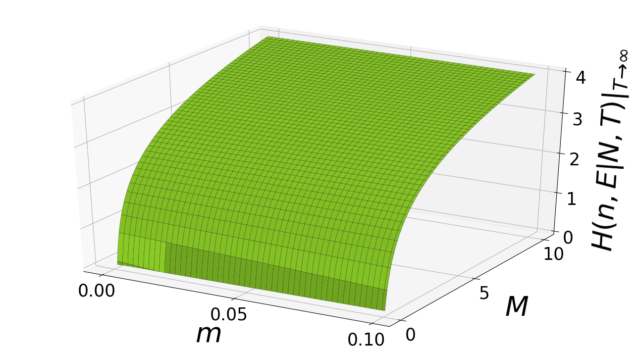
Figure 4: (Color online) High-temperature asymptotics of the entropy $H(n,E|N,T)$ of Unruh radiation given by Eq. (27) for fermions $(N=2)$ as function of $m$ and $M$.

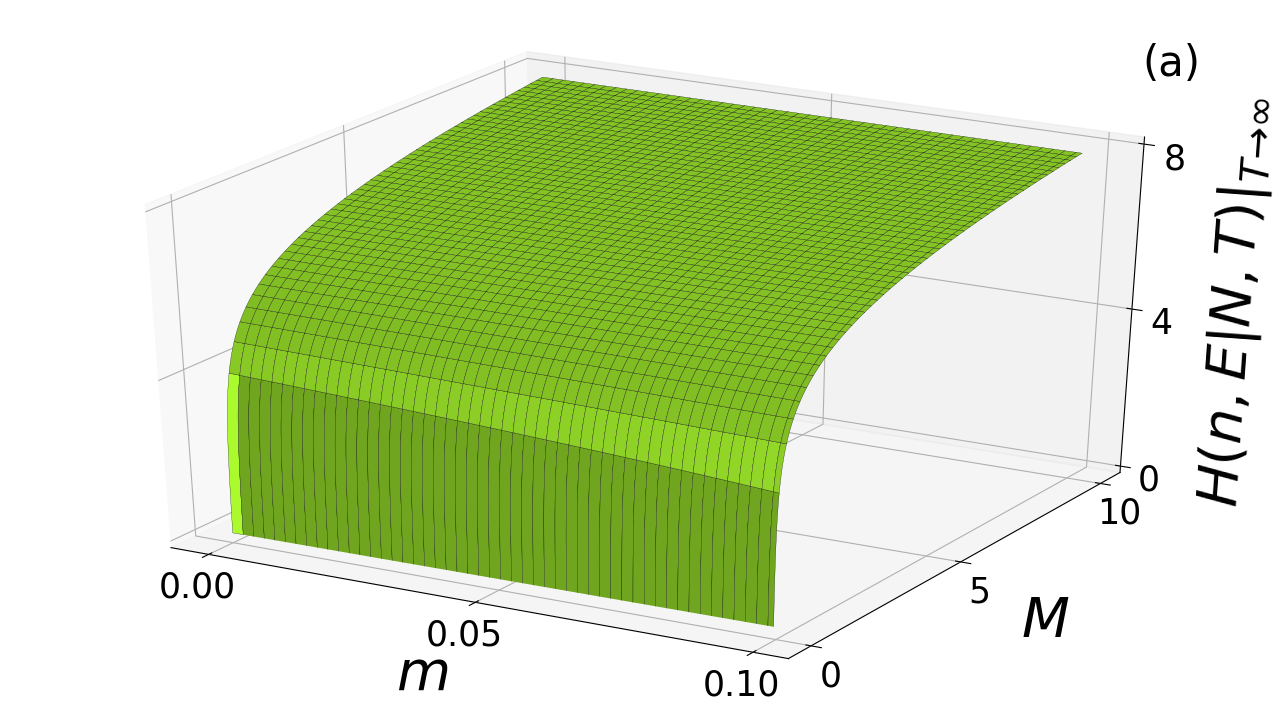
Figure 5: (Color online) The same as Fig. 4 but for bosons with (a) $N=100$ and (b) $N=1000$ particles in the spectrum.

VI Generalization to intrinsic degrees of freedom

Expression (16) is valid for some mode of the radiated field only, which is defined by joint multiplicity-energy distribution $\left\{n,E\right\}$, temperature $T$ and parameter $N$. However, since the emitted particles may have additional degrees of freedom $\{\lambda\}$, such as electric charge, spin, polarization etc., they have to be taken into account too. This is equivalent to the following modification of the total distribution

$$\left\{n,E|N,T\right\}\to\left\{\lambda,n,E|N,T\right\}.$$

Using Eq. (5) we obtain then

$$H\left(\lambda,n,E|N,T\right)=H\left(\lambda\right)+\Braket{H\left(n,E}{N,T,\lambda}_{\lambda}.$$ (28)

But such a generalization is not an easy task at all. Let us consider a simple example. While detecting particle at some $E$ one should measure its energy. Such a process results in consumption of the particle’s momentum. One may argue that calorimetry is not required. The observer can build some source of similar particles and carry out interference experiments to determine energy of the particle to be detected. But any such interference will result in re-distribution of the momenta during interference, and therefore will change the observer’s momentum as well. Thus one concludes that measuring the particle’s energy $E$ leads to change of the observer’s acceleration $a$. It implies change of Unruh temperature $T=a/\left(2\pi\right)$ of the source the observer is dealing with.

One may also note that Unruh effect is being considered in case of quasi-classical approach. It means that the density matrix $\rho_{\rm out}$ in Eq. (9) is obtained under assumption that the outgoing radiation makes no influence on the background metric, see [4, 24, 25]. Such a remark is correct, but what about other degrees of freedom $\lambda$? For instance, taking into account spin of the particles emitted by the Unruh horizon may lead to change of the observer’s angular momentum. In this case the observer’s acceleration $a$ can not be constant due to conservation of the total angular momentum anyway and thus implies change of $T$ in Eq. (28) during particle identification.

So, the situation seems to be simple only if one neglects any influence of the outgoing particles during the Unruh effect. In this case the entropy $H\left(n,E|N,T,\lambda\right)$ does not depend on $\left\{\lambda\right\}$, and expression (28) is reduced to the sum

$$H\left(\lambda,n,E|N,T\right)=H\left(\lambda\right)+H\left(n,E|N,T\right).$$ (29)

VII Conclusions

The Unruh effect is considered from the point of view of information theory. We estimated the total entropy of the radiation generated by the Unruh horizon in the non-inertial reference frame for the state verified as vacuum by any inertial observer. Usually such a case is treated as von Neumann entropy of the corresponding density matrix. But this is just the starting point of our study, because the density matrix of outgoing radiation describes conditional multiplicity distribution at given energy and Unruh temperature. As a result, it allows one to estimate total entropy of the Unruh source by taking into account both multiplicity and energy distribution of the outgoing quanta. We show how it can be calculated even without exact knowledge of the corresponding Hamiltonian. In particular, such a lack of information results in Schwinger-like spectrum of the emission, see Eq. (14).

The case of finite amount of particle emission is considered. It allows us to utilize the results for realistic particle emission spectra. Asymptotics of the general expression for entropy with respect to low and high values of Unruh temperature are also investigated. We found that in case of small acceleration, corresponding to low temperature, entropy of the radiation does not depend on maximal amount of emitted particles in the leading order, see Eq. (22). Dependence on $N$ is recovered for large accelerations, when $T\to\infty$, see Eq. (27). It can be explained by abundant emission of particles from the hot Unruh horizon, when amount of the emitted quanta may be considered as extra degree of freedom contributing to the total entropy.

Another interesting point is that the total entropy $H\left(n,E|N,T\right)$ quickly drops to zero with increase of the mass $m$ of the quanta. It can be explained by the energy conservation law: the more energy is being spent on creation of particle’s mass, the less of it may be used to generate total distribution. At the same time, total entropy of the Unruh source slightly increases with the maximum allowed energy $M$, because the distribution widens with increase of $M$ thus leading to the total entropy increase.

The obtained results can be applied to analysis of particle distributions in inelastic scattering processes at high energies. Also, they may be generalized to other degrees of freedom of the emitted particles, such as spin, charges etc. However, such a generalization may significantly complicate the analysis. For instance, additional conservation laws originating from the other degrees of freedom might change the metric. Therefore, one may be forced to take distribution $\left\{T\right\}$ into account too.

- [1] W.G. Unruh, Notes on black-hole evaporation, Phys. Rev. D 14, 870 (1976).
- [2] S.W. Hawking, Particle creation by black holes, Comm. Math. Phys. 43, 199 (1975).
- [3] J.D. Bekenstein, Black holes and entropy, Phys. Rev. D 7, 2333 (1973); Statistical black-hole thermodynamics, ibid. 12, 3077 (1975).
- [4] L.C.B. Crispino, A. Higuchi, and G.E.A. Matsas, The Unruh effect and its applications, Rev. Mod. Phys. 80, 787 (2008).
- [5] N. Obadia and M. Milgrom, On the Unruh effect for general trajectories, Phys. Rev. D 75, 065006 (2007).
- [6] J.I. Korsbakken and J.M. Leinaas, The Fulling-Unruh effect in general stationary accelerated frames, Phys. Rev. D 70, 084016 (2004).
- [7] S. Takagi, Vacuum noise and stress induced by uniform acceleration: Hawking-Unruh effect in Rindler manifold of arbitrary dimension, Prog. Theor. Phys. Suppl. 88, 1 (1986).
- [8] J.J. Bisognano and E.H. Wichmann, On the duality connection for a Hermitian scalar field, J. Math, Phys. 16, 985 (1975); On the duality connection for quantum fields, ibid. 17, 303 (1976).
- [9] W.G. Unruh and N. Weiss, Acceleration radiation in inteacting field theories, Phs. Rev. D 29, 1656 (1984).
- [10] F. Becattini, Thermodynamic equilibrium with acceleration and the Unruh effect, Phys. Rev. D 97, 085013 (2018).
- [11] F. Becattini and D. Rindori, Extensivity, entropy current, area law and Unruh effect, Phys. Rev. D 99, 125011 (2019).
- [12] G.Y. Prokhorov, O.V. Teryaev, and V.I. Zakharov, Unruh effect for fermions from the Zubarev density operator, Phys. Rev. D 99, 071901 (2019).
- [13] D.N. Zubarev, A.V. Prozorkevich, and S.A. Smolyanskii, Derivation of nonlinear generalized equations of quantum relativistic hydrodynamics, Theor. Math. Phys. 40, 821 (1979).
- [14] F. Becattini, M. Buzzegoli, and F. Grossi, Reworking the Zubarev’s approach to non-equilibrium quantum statistical mechanics, arXiv:1902.01089.
- [15] B.F. Svaiter and N.F. Svaiter, Inertial and noninertial particle detectors and vacuum fluctuations, Phys. Rev. D 46, 5267 (1992).
- [16] L. Sriramkumar and T. Padmanabhan, Response of finite time particle detectors in noninertial frames and cirved space-time, Class. Quant. Grav. 13, 2061 (1996).
- [17] P. Chen and T. Tajima, Testing Unruh radiation with ultraintense lasers, Phys. Rev. Lett 83, 256 (1999).
- [18] J. Louko and A. Satz, Transition rate of the Unruh-DeWitt detector in curved spacetime, Class. Quant. Grav. 25, 055012 (2008).
- [19] V. Akhmedova, T. Pilling, A. de Gill, D. Singleton, Comments on anomaly versus WKB/tunneling methods for calculating Unruh radiation, Phys. Lett. B 673, 227 (2008).
- [20] K. Bradler, Eavesdropping of quantum communication from a non-inertial frame, Phys. Rev. A 75, 022311 (2007).
- [21] M. Han, S.J. Olson, and J.P. Dowling, Generating entangled photons from the vacuum by accelerated measurements: Quantum information theory meets the Unruh-Davies effect, Phys. Rev. A 78, 022302 (2008).
- [22] R. Parentani and S. Massar, The Schwinger mechanism, the Unruh effect and the production of accelerated black holes, Phys. Rev. D 55, 3603 (1997).
- [23] J.S. Bell and J.M. Leinaas, Electrons as accelerated thermometers, Nucl. Phys. B 212, 131 (1983).
- [24] R. Banerjee and B.R. Majhi, Hawking black body spectrum from tunneling mechanism, Phys. Lett. B 675, 243 (2009).
- [25] D. Roy, The Unruh thermal spectrum through scalar and fermion tunneling, Phys. Lett. B 681, 185 (2009).
- [26] S. Barshay and W. Troost, A possible origin for temperature in strong interactions, Phys. Lett. 73B, 437 (1978).
- [27] A.F. Grillo and Y. Srivastava, Intrinsic temperature of confined systems, Phys. Lett. B 85, 377 (1979).
- [28] A. Hosoya, Moving mirror effects in hadronic reactions, Progr. Theor. Phys. 61, 280 (1979).
- [29] S. Barshay, H. Braun, J.P. Gerber, and G. Maurer, Possible evidence for fluctuations in the hadronic temperature, Phys. Rev. D 21, 1849 (1980).
- [30] D. Kharzeev and K. Tuchin, From color glass condensate to quark gluon plasma through the event horizon, Nucl. Phys. A 753, 316 (2005).
- [31] P. Castorina, D. Kharzeev, and H. Satz, Thermal hadronization and Hawking-Unruh radiation in QCD, Eur. Phys. J. C 52, 187 (2007).
- [32] P. Castorina and H. Satz, Hawking-Unruh hadronization and strangeness production in high energy collisions, Adv. High Energy Phys. 2014, 376982 (2014).
- [33] T.S. Biro, M. Gyulassy, and Z. Schram, Unruh gamma radiation at RHIC?, Phys. Lett. B 708, 276 (2012).
- [34] Proceedings of Quark Matter 2019, edited by F. Liu, E. Wang, X.-N. Wang, N. Xu, and B.-W. Zhang, Nucl. Phys. A 1005, 122104 (2021).
- [35] Proceedings of Quark Matter 2018, edited by F. Antinori, A. Dainese, P. Giubellino, V. Greco, M.P. Lombardo, and E. Scomparin, Nucl. Phys. A 982, 1-1066 (2019).
- [36] D. Marolf, D. Minic, and S.F. Ross, Notes on spacetime thermodynamics and the observer dependence of entropy, Phys. Rev. D 69, 064006 (2004).
- [37] E.T. Jaynes, Information theory and statistical mechanics, in Lectures in Theoretical Physics. Vol. 3. Statistical Physics, edited by K.W. Ford (Benjamin, NY, 1963), p. 181.
- [38] E.T. Jaynes, Prior probabilities, IEEE Trans. on Systems Science and Cybernetics, SSC-4, 227 (1968).
- [39] A. Pathak, Elements of Quantum Computation and Quantum Communication, (Taylor & Francis, London, 2013).
- [40] J. Schwinger, On Gauge Invariance and Vacuum Polarization, Phys. Rev. 82, 664 (1951).