Dark Energy and Cosmological Horizon Thermal Effects

Abstract

We investigate various dark energy models by taking into account the thermal effects induced from Hawking radiation on the apparent horizon of the Universe, for example near a finite-time future singularity. If the dark energy density increases as the Universe expands, the Universe’s evolution reaches a singularity of II type (or sudden future singularity). The second derivative of scale factor diverges but the first remains finite. Quasi-de Sitter evolution can change on sudden future singularity in the case of having an effective cosmological constant larger than the maximum possible value of the energy density of the Universe. Another interesting feature of cosmological solution is the possibility of a transition between deceleration and acceleration for quintessence dark energy with a simple equation of state. Finally, we investigate which fluid component can remedy Big Rip singularities and other crushing type singularities.

I Introduction

The accelerated expansion of the Universe Riess ; Perlmutter from a theoretical viewpoint can be caused by some fluid with negative pressure and/or negative entropy (for review, see Bamba:2012cp ; Dark-6 ; Cai:2009zp ). Due to the fact that it is still unknown how this fluid will behave, the late-time accelerated expansion era is dubbed the dark energy era. The current observations coming from Planck Akrami:2018odb , indicate that dark energy controls nearly 70% of total energy density of the Universe Kowalski . The equation of state (EoS) parameter for the dark fluid, namely $w_{d}$, is negative, that is,

$$w_{\mathrm{d}}=p_{d}/\rho_{d}<0,$$ (1)

where $\rho_{d}$ and $p_{d}$ are the dark energy density and pressure correspondingly. However, it is still not clear what is the precise value of $w_{d}$ PDP ; Amman , although the latest Planck data constraint significantly the values that the EoS parameter can take. The standard $\Lambda$-Cold-Dark-Matter ($\Lambda$CDM) model according to which dark energy is simply a cosmological constant, implies that $w_{d}=-1$. If the EoS parameter is in the range $-1<w_{d}<-1/3$ the evolution of the Universe is quintessential. An interesting case (although controversial Carrol ) arises for $w_{d}<-1$, and in this case the Universe evolves dominated by phantom dark energy. A simple choice of the form $w_{d}=\mbox{const}$ leads to a Big-Rip singularity Caldwell ; Caldwell-2003 ; Carrol ; P ; Frampton ; Nojiri:2003vn ; Faraoni:2001tq ; GonzalezDiaz:2003rf ; Elizalde:2004mq ; Singh:2003vx ; Csaki:2004ha ; Wu:2004ex ; Nesseris:2004uj ; Stefancic:2003rc ; Chimento:2003qy ; Hao:2004ky ; Dabrowski:2004hx ; Nojiri , where the scale factor and all the physical quantities that can be defined on the three dimensional spacelike singularity defined of the time instance that the Rip occurs, severely diverge. There are other types of singularities for phantom Universe, for example a singularity of type III corresponds to a situation in which, the Hubble parameter $H$ diverges at a finite time and for a finite scale factor. A sudden future singularity (or type II) is milder in comparison with the two previous. The scale factor and its first derivative (and therefore the energy density) are finite at the moment of the singularity, but the second derivative of scale factor diverges (and the pressure correspondingly) Barrow ; Shtanov:2002ek ; Nojiri:2004ip ; Cotsakis:2004ih ; Dabrowski:2004bz ; FernandezJambrina:2004yy ; FernandezJambrina:2008dt ; Barrow:2004he ; Stefancic:2004kb ; Cattoen:2005dx ; Tretyakov:2005en ; Balcerzak:2006ac ; Yurov:2007tw ; Barrow:2009df ; BouhmadiLopez:2009jk . This singularity can occur for quintessential evolution too. In principle, the occurrence of finite-time singularities, during the evolution of the Universe, is not necessarily a consequence of phantom dark energy. In fact, a phantom scalar field always leads to a Big Rip singularity Caldwell , but the opposite is not true. For some studies on alternative models leading to a little-rip singularity, see Refs. Frampton-2 ; Frampton:2011aa ; Frampton-3 ; Astashenok . If the EoS parameter $w$ tends to minus unity sufficiently fast, the time instance that the singularity occurs is at infinity. Of course, by that time, the tidal forces would grow infinitely large and all the stellar structures and galactic structures would be torn apart by the tidal forces before the singularity would ever be reached. Another possibility is the so-called pseudo-rip scenario, which can be realized when the energy density of dark energy approaches asymptotically a constant value (effective “cosmological constant”). This effective “cosmological constant” in principle can considerably differ from the current energy density of dark energy $\rho_{d0}$.

According to the observational data, it is marginally probable that the phantom divide line is crossed and the dark energy era is actually a phantom dark energy era. For example for the flat $wCDM$ model according to latest Planck data, the dark energy EoS is constrained as follows,

$$w=-0.978\pm 0.059\,,$$

so the possibility $w<-1$ is not excluded, and the dark energy era is a probable scenario. But for $w<-1$ future finite time singularities can occur. Therefore, the occurrence of future finite time singularities is a realistic possibility, even present in the context of Einstein-Hilbert gravity by using phantom scalar fields Caldwell-2003 . When a finite-time singularity is approached, it is natural to assume that several effects having to do with the cosmological horizon surrounding the singularity, should be taken into account. The crushing-type finite-time singularities are somewhat similar to black hole singularities, in the sense that these are both future spacelike singularities. In this sense, it is natural to assume that the cosmological horizon would cause some cosmological effects on the evolution of the Universe, near the singularity, exactly as in the black holes case. Particularly, using the analogy with Hawking radiation from black holes one can consider thermal radiation from horizon of the Universe Gibbons , Cai . In Rugg it was argued that the kind of cyclic cosmology might be realized instead of the Big Rip singularity due to effect of thermal radiation. In this paper we shall consider the effects of thermal cosmological horizon terms, generalizing the work of Nojiri:2020sti , and for the dark energy we shall assume that it will have a generalized EoS of the form $p_{d}=g(\rho_{d})$, where $g$ is an arbitrary function. We shall consider various models of dark energy with the inclusion of thermal radiation effects. After discussing the main theoretical framework, we shall study two important state-finder parameters, namely the deceleration and jerk parameters. Then some simple dark energy EoS parameters are considered, with account of thermal radiation. Also our findings show that for any equation of state which leads to infinitely increasing phantom energy density, a sudden future singularity always occurs. Also the little rip regime cannot be realized in the present framework, and interestingly enough only one scenario of non-singular evolution for phantom energy takes place, that of pseudo-rip evolution, but in that case, the value of the ”effective” cosmological constant should be less than some critical density. It is also important to note that in the present context, a phantom dark energy era can be realized without the need for a phantom scalar field, as in ordinary Einstein-Hilbert gravity.

II Field Equations and the Description of the Theoretical Framework

In this section we briefly consider the cosmological equations for the evolution of the Universe, by taking into account the thermal radiation effects from the cosmological horizon. Let’s start from the spatially-flat FRW universe with metric,

$$ds^{2}=dt^{2}-a^{2}(t)(dx^{2}+dy^{2}+dz^{2}).$$ (2)

The cosmological equations are,

$$\left(\frac{\dot{a}}{a}\right)^{2}=\frac{\rho}{3}\,,\quad\frac{\ddot{a}}{a}=-\frac{1}{6}(\rho+3p)\,,$$ (3)

where $\rho$ and $p$ are the total energy density and pressure, $a$ is the scale factor,and the “dot” denotes differentiation with respect to the cosmic time. We use the system of units in which $8\pi G=c=1$, the so-called reduced Planck units system.

From the Friedmann and the Raychaudhuri equations it follows that,

$$\dot{\rho}+3H(\rho+p)=0.$$ (4)

If the Universe consists of non-interacting components $\rho_{i}$, this equation holds for each component $\rho_{i}$.

The radius of the apparent horizon of the Universe is

$$r_{h}\sim 1/H\,,$$

Therefore, the Hawking temperature of the thermal radiation appearing due to the apparent horizon is proportional to Hubble parameter $H$. The energy density of radiation thermal term according to Stefan-Boltzmann law is,

$$\rho_{t_{rad}}=3\alpha H^{4}\,,$$

where $\alpha$ is some constant. The multiplicative factor 3 is introduced for convenience. One can expect that the constant $\alpha$ could be calculated from a self-consistent quantum model describing the thermal radiation. Such a model though is not available, and therefore the direct usage of the thermal radiation effects related to the de Sitter horizon is not justified. However, in order to have a concrete idea of these effects, we assumed only by analogy that the energy density of thermal radiation is proportional to $H^{4}$, because the temperature of Hawking radiation of the apparent horizon is inversely proportional to the size of the horizon.

A similar physical analogy is used in the context of holographic energy, for which we usually assume that,

$$\rho=\beta/L^{2}\,,$$

where $L$ is the event horizon. Regarding the values of $\beta$, there are various estimations from calculations, but its exact value is unknown. Therefore we use $\alpha$ as the unknown parameter in our calculations.

The Friedmann equation for the Hubble parameter, by taking into account the density of thermal radiation, is,

$$\alpha H^{4}-H^{2}+\frac{\rho}{3}=0\,,$$ (5)

which can be solved with respect to the Hubble parameter as follows,

$$H=\pm\left(\frac{1\pm\sqrt{1-4\alpha\rho/3}}{2\alpha}\right)^{1/2}\,.$$ (6)

Further we assume that the Universe expands, and therefore the sign “+” is chosen. One also needs to choose sign “-” in brackets for the following reason. Seing the thermal radiation as the Hawking radiation from the apparent horizon has a quantum origin. It is known that the cosmological evolution of Universe from beginning to present date, is described well by the Friedmann equations and one can expect that for $\alpha\rightarrow 0$ (Universe without thermal radiation) we should obtain the ordinary Friedmann equations. And for $\alpha\rho/3<<1$, we obtain the ordinary cosmological model,

$$H^{2}=\frac{1-\sqrt{1-4\alpha\rho/3}}{2\alpha}\approx\frac{1-(1-2\alpha\rho/3)}{2\alpha}=\frac{\rho}{3}.$$

But by choosing “+”, we obtained very strange cosmological model with a Hubble parameter which tends to infinity for $\alpha\rightarrow\infty$.

For these choices of signs in Eq. (6), one can obtain the following relation for the derivative of Hubble parameter,

$$\dot{H}=-\frac{1}{2}\frac{\rho+p}{\sqrt{1-4\alpha\rho/3}}.$$ (7)

The second derivative of the scale factor is,

$$\frac{\ddot{a}}{a}=\dot{H}+H^{2}=-\frac{1}{2}\frac{\rho+p}{\sqrt{1-4\alpha\rho/3}}+\frac{1-\sqrt{1-4\alpha\rho/3}}{2\alpha}.$$ (8)

We consider the case when equation of state for dark energy is given in form,

$$p_{\mathrm{d}}=-\rho_{\mathrm{d}}-f(\rho_{\mathrm{d}})\,,$$ (9)

where $f(\rho_{\mathrm{d}})$ is some arbitrary function. Condition $f(\rho)>0$ corresponds to phantom energy while for $f(\rho)<0$, describes the case of quintessential evolution.

For the case of dominating of dark energy we can don’t consider other components of matter. In this case from the equation for Hubble parameter and Eq. (4), one can get the relation for cosmological time,

$$t=\frac{\sqrt{2\alpha}}{{3}}\int^{\rho}_{\rho_{0}}\frac{d\rho}{f(\rho)\left(1-\sqrt{1-4\alpha\rho/3}\right)^{1/2}}.$$ (10)

We omit the subscript $\mathrm{d}$ in this relation assuming $\rho=\rho_{d}$. The quintessence energy density decreases with time ($\rho<\rho_{0}$), while the phantom energy density increases ($\rho>\rho_{0}$).

The effective pressure and density can be defined as,

$$\rho_{eff}=3H^{2},\quad p_{eff}=-2\dot{H}-3H^{2}$$ (11)

and therefore for our cosmological model we have,

$$\rho_{eff}=\frac{3}{2\alpha}\left(1-\sqrt{1-4\alpha\rho/3}\right),$$ (12)

$$p_{eff}=\frac{\rho+p}{\sqrt{1-4\alpha\rho/3}}-\rho_{eff}.$$

From this relation one can conclude that the effective pressure reaches infinity for a finite value of the energy density $\rho_{max}=\frac{3}{4\alpha}$ (the effective energy density is finite also). Therefore, we have a type II singularity (or sudden future singularity in another words). We can also compute the scale factor as,

$$a=a_{0}\exp\left(\frac{1}{3}\int^{\rho}_{\rho_{0}}\frac{d\rho}{f(\rho)}\right)\,.$$ (13)

From Eq. (10) one can see that there are two main possibilities for the cosmological evolution,

1. The integral (10) converges at $\rho\rightarrow\rho_{m}=\frac{3}{4\alpha}$ and singularity of type II takes place Barrow ; Nojiri-2 .

   The scale factor remains finite with its first derivative with respect to the cosmic time. This variant of cosmological evolution is realized for phantom dark energy only. Also we have singularity of this type if $f(\rho)$ has a zero at some $\rho_{f}<\rho_{m}$ and the integral with respect to the cosmic time converges.

2. Although we do not know the equation of state for dark energy, we can forecast its qualitative behavior by assuming that the function $f(\rho)$ has a zero at some value $\rho_{f}$. If the integral (10) diverges at some value of energy density $\rho\rightarrow\rho_{f}<\frac{3}{4\alpha}$. In this case scale factor tends to infinity at $t\rightarrow\infty$. Therefore we have quasi-de Sitter expansion with effective cosmological constant $\Lambda=\rho_{f}$.

Of course one can ask how it is possible to discriminate the effects of the thermal radiation from modified gravity or specific fluid effects. This question arises for many cosmological models. Theories of modified gravity can lead to cosmological dynamics similar to models with some fluids or models on brane for example. Maybe one of the arguments is in favor for the model of thermal radiation which is inherently relatively simpler (on our opinion of course) in comparison with complicated form of actions of Galileon gravity for example.

One of the main indicators for any cosmological model is data about distance modulus as a function of the redshift from the Supernova Cosmology Project Amanullah:2010vv . For standard cosmology the distance modulus for a supernova with redshift $z=a_{0}/a-1$ is

$$\mu(z)=\mbox{const}+5\log D_{L}(z).$$ (14)

Here $D_{L}(z)$ is the luminosity distance. For Friedmann cosmology, the luminosity distance is,

$$D_{L}(z)=\frac{c}{H_{0}}(1+z)\int_{0}^{z}\frac{dz}{E(z)},$$ (15)

where $E(z)$ is the dimensionless Hubble parameter i.e.

$$E(z)=\frac{H(z)}{H_{0}}=\left(\frac{\rho}{\rho_{0}}\right)^{1/2}.$$

In particular, for the well known $\Lambda$CDM model, we have,

$$E(z)=\left(\Omega_{m}(1+z)^{3}+\Omega_{\Lambda}\right)^{1/2}.$$ (16)

Here, $\Omega_{m}$ is the fraction of the total density contributed by matter, and $\Omega_{\Lambda}$ is the fraction contributed by the vacuum energy density.

For our purposes, it is convenient to use dimensionless units for the Hubble parameter, $\alpha$ and energy density:

$$\alpha\rightarrow\tilde{\alpha}H_{0}^{-2},\quad H\rightarrow H_{0}E,\quad\rho\rightarrow 3H_{0}^{2}\tilde{\rho}.$$

In these units for dimensionless Hubble parameter, we obtain,

$$E=\left(\frac{1-\sqrt{1-4\tilde{\alpha}\tilde{\rho}}}{2\tilde{\alpha}}\right)^{1/2}.$$ (17)

One needs to take into account that, at present time, the dimensionless density satisfies $\tilde{\rho}_{0}\neq 1$, in contrast with the ordinary Friedmann cosmological model, because $\rho_{0}\neq 3H_{0}^{2}$ although for $\tilde{\alpha}<<1$ one can assume that $\tilde{\rho}_{0}\approx 1$.

The deceleration parameter $q_{0}$ is defined according to relation,

$$q=-\frac{1}{aH^{2}}\frac{d^{2}a}{dt^{2}}=$$ (18)

$$=-1+{\alpha}\left(1-4\alpha\rho/3\right)^{-1/2}\left(1-(1-4\alpha\rho/3)^{1/2}\right)^{-1}(\rho+p)$$

In Friedmann cosmology one obtains the well-known expression for $q$ assuming simply $\alpha\rightarrow 0$ in the following equation,

$$q^{(0)}=-1+\frac{3}{2}\left(1+\frac{p}{\rho}\right).$$ (19)

For the $\Lambda$CDM model one obtains,

$$q^{(0)}_{\Lambda CDM}=-1+\frac{3}{2}\Omega_{m}.$$

One can get also jerk parameter $j$ Sahni:2002fz for our model in comparison with ordinary cosmology,

$$j=\frac{1}{aH^{3}}\frac{d^{3}a}{dt^{3}}=$$ (20)

$$=2\alpha\left(\frac{\alpha(\rho+p)^{2}}{(1-4\alpha\rho/3)^{3/2}}+\frac{1-\sqrt{1-4\alpha\rho/3}}{2\alpha}+\frac{3(\rho+p)}{2(1-4\alpha\rho/3)^{1/2}}\frac{dp}{d\rho}\right)(1-(1-4\alpha\rho/3)^{1/2})^{-1}$$

For $\alpha\rightarrow 0$ we get,

$$j^{(0)}=1+\frac{9}{2}\left(1+\frac{p}{\rho}\right)\frac{dp}{d\rho}$$ (21)

and particularly for the $\Lambda$CDM model we have $p=-\Lambda=\mbox{const}$, therefore $j^{(0)}_{\Lambda CDM}=1$.

Data about the deceleration and jerk parameters can be obtained from astronomical observations of distant objects at redshifts $z\gtrsim 1$. Estimations for deceleration and jerk parameter from current observations do not discriminate directly the correct model of dark energy, because statistical errors are sufficiently large, and therefore models alternative to the $\Lambda$CDM model can be perfectly compatible to the current observational data. The $\Lambda$CDM values of these statefinder quantities can act as reference points for alternative to $\Lambda$CDM models.

In the next sections, we shall present several dark energy models by taking into account thermal radiation effects.

There are various scenarios for a Universe with dark energy in the future. From observations it is apparent that equation of state for dark energy is very close to simple equation of state of the cosmological constant,

$$p_{d}=-\rho_{d}.$$

It is convenient to use EoS formalism for other models of dark energy. Such formalism can be applied not only to models in which dark energy is a fluid but for scalar fields too. Our main purpose was to investigate the role which thermal radiation in these scenarios. Therefore the models that we shall study in the following sections, are illustrative and simple examples of dark energy models with a variety of possible future evolutions, with a common characteristic though, that they mimic the standard cosmological model in the cosmological past.

III A Decelerating Quintessence Model

It is well-known that for a quintessential Universe with simple equation of state $p=w\rho$ ($-1<w<-1/3$), only acceleration takes place. By taking into account the thermal radiation effects, allows us to construct models with a phase of deceleration in the past, emerging from sudden finite-time singularities. Such Universe emerges from a sudden finite-time singularity in the past. The initial value of the Hubble parameter is,

$$H_{i}=\frac{1}{\sqrt{2\alpha}},$$ (22)

and the energy density of quintessence at the moment of the singularity is,

$$\rho_{i}=\frac{3}{4\alpha}$$ (23)

and then it decreases with scale factor as,

$$\rho_{d}=\frac{\rho_{i}a_{i}^{3(w+1)}}{a^{3(w+1)}}.$$

Therefore we have,

$$\frac{\ddot{a}}{a}=-\frac{1}{2}\frac{\rho_{i}(1+w)}{\sqrt{1-a_{i}^{3(w+1)}/a^{3(w+1)}}}\frac{a_{i}^{3(w+1)}}{a^{3(w+1)}}+\frac{1-\sqrt{1-a_{i}^{3(w+1)}/a^{3(w+1)}}}{2\alpha}\,.$$ (24)

For $t>>t_{i}$ we have,

$$\frac{\ddot{a}}{{a}}=-\frac{1}{6}(1+3w)\rho_{i}a_{i}^{3(w+1)}/a^{3(w+1)}>0.$$

Near the initial singularity, the first term in Eq. (24) is very large and negative for quintessence, and therefore $\ddot{a}<0$. Eventually a deceleration to acceleration transition occurs, at some later time instance. Of course this cosmological model is not realistic, since we did not aim to confront it with the observational data. It is a rather qualitative model, showing that a decelerating quintessential model which evolves to an accelerating state, is possible to be realized by taking into account thermal effects.

In Fig. 1 we depicted dependence of acceleration from scale factor for various $w$ and $\alpha$. Duration of decelerating phase depends from $w$ strongly. In a phantom case first term is always positive and therefore universe filled phantom energy expands with acceleration.

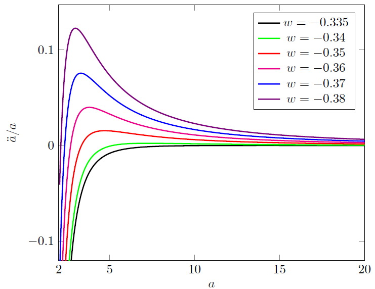
Figure 1: Dependence of acceleration $\ddot{a}/a$ (in units of $H_{0}^{2}$ from scale factor for various values of $w$ in a case of simple model of quintessence with constant parameter of state. For $\tilde{\alpha}$ we take value 0.01. Initial value of scalar factor is $a_{i}=1$. Duration of phase with $\ddot{a}<0$ decreases for larger $|w|$. Maximal value of acceleration otherwise increases.

IV Transition from Little-Rip and Type I and III Singularities to type II Singularity

Let’s consider the case of the following EoS,

$$f(\rho_{d})=\beta^{2}\rho_{d0}(\rho_{d}/\rho_{d0})^{\gamma},\quad\beta,\gamma\equiv\mbox{const}>0.$$ (25)

In Friedmann cosmology without radiation term, this EoS leads to various scenarios of cosmological evolution: 1) little rip takes place for $\gamma\leq 1/2$ Frampton-2 -Astashenok ; 2) $1/2<\gamma\leq 1$ corresponds to Big Rip singularity and 3) for $\gamma>1$ we have a Type III singularity. The EoS parameter $w=p_{d}/\rho_{d}$ for the above EoS at present time is simply,

$$w_{0}=-1-\beta^{2}.$$

In our case we have only Type II singularity for this EoS. We start our consideration using a simple model:

$$f(\rho)=\beta^{2}\rho_{d0}=\mathrm{const}\,.$$ (26)

From the continuity equation for the dark energy fluid (3) we derive

$$\rho_{d}=\rho_{d0}(1+3\beta^{2}\ln a).$$ (27)

Without loss of generality we assume that the current value of the scale factor is $a_{0}=1$. We consider the Universe filled matter and dark energy only and calculate the time for the final singularity for several values of $w_{0}$ and $\alpha$. Also we considered the behavior of cosmological acceleration in past and we found the time instance at which $\ddot{a}$ changes sign, and our results are presented in 1.

	$w_{0}=-1.05$		$w_{0}=-1.075$		$w_{0}=-1.10$
$\tilde{\alpha}$	$t_{\mathrm{f}}-t_{0}$	$t_{0}-t_{a}$	$t_{\mathrm{f}}-t_{0}$	$t_{0}-t_{a}$	$t_{\mathrm{f}}-t_{0}$	$t_{0}-t_{a}$
0.001	144.64	0.467	119.21	0.468	103.40	0.470
0.005	107.69	0.460	71.77	0.462	53.82	0.464
0.01	71.54	0.452	47.67	0.454	35.74	0.456
0.02	45.99	0.435	30.64	0.438	22.97	0.440
0.05	23.36	0.386	15.55	0.390	11.65	0.394

Table 1: Time for singularity $t_{f}-t_{0}$ and time after moment when acceleration began $t_{0}-t_{a}$ (in units of $H_{0}^{-1}$) for various values of $\tilde{\alpha}$). For initial $\Omega_{m}$ the value 0.28 is taken.

The behavior of the deceleration $q$ and jerk $j$ parameters are presented in Fig. 2 in comparison with dark energy model (25) without thermal radiation from the moment of beginning of cosmological acceleration.

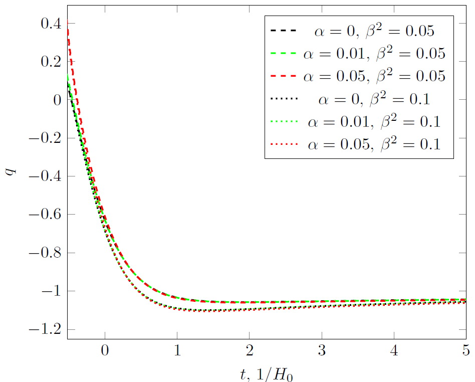
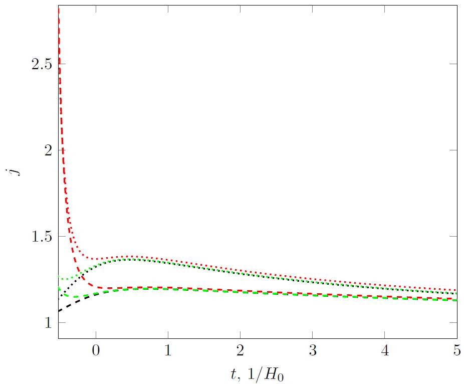
Figure 2: Deceleration (left panel) and jerk (right panel) parameters in model (26) for some $\beta^{2}$ and $\alpha$. Hereinafter for $\Omega_{d0}$ is taken 0.72 in current moment.

Roughly, one can expect that thermal radiation effects have a measurable effect, only during the cosmological acceleration.

One can describe this model in terms of scalar field theory, and in the case of a phantom scalar field, the energy density and the pressure of the scalar field are,

$$\rho_{d}=-\frac{\dot{\phi}^{2}}{2}+V(\phi),\quad p_{d}=-\frac{\dot{\phi}^{2}}{2}-V(\phi).$$ (28)

, From these equations one can obtain that

$$\phi=\int\sqrt{-\rho_{d}-p_{d}}dt=\int\sqrt{f(\rho_{d})}dt.$$ (29)

For $f(\rho)$ from Eq. (26) we have simple linear dependence of scalar field with respect to the cosmic time,

$$\phi=\phi_{0}+\beta\sqrt{\rho_{d0}}t.$$ (30)

For a Universe dominated of dark energy without thermal radiation,

$$t=\sqrt{3}\int\frac{da}{a\sqrt{\rho_{d}}}$$ (31)

and thus we have for the integral (27),

$$t=\frac{1}{\mu}\left({1+3\beta^{2}\ln a}-1\right),\quad\mu\equiv\frac{\beta^{2}\sqrt{3\rho_{d0}}}{2}.$$

For the scalar field potential we have,

$$2V=\rho_{d}-p_{d}=2\rho_{d}+f(\rho_{d})=2\rho_{d0}\sqrt{1+3\beta^{2}\ln a}+\beta^{2}\rho_{d0}.$$

Using the expression for the cosmic time, one obtains the potential as function of scalar field has the following form,

$$V(\phi)=\frac{3\beta^{2}}{4}(\phi-\phi^{*})^{2}+\frac{\beta^{2}\rho_{d0}}{2},\quad\phi^{*}\equiv\phi_{0}-\frac{2}{\sqrt{3}\beta}$$ (32)

With thermal radiation we have for the cosmic time a more complicated expression,

$$t=\frac{1}{\nu}\left\{\left(2+g(x)\right)\sqrt{1-g(x)}-\left(2+g(0)\right)\sqrt{1-g(0)}\right\},\quad g(x)\equiv\sqrt{1-4\alpha\rho_{d0}/3-4\alpha\beta^{2}x},$$ (33)

$$x\equiv\ln a,\quad\nu\equiv\frac{3\sqrt{\alpha}\beta^{2}\rho_{d0}}{\sqrt{2}}.$$

Therefore, the potential of scalar field could be obtained only in parametric form. For comparison we present the dependence of the potential with respect to various parameters in Fig. 3.

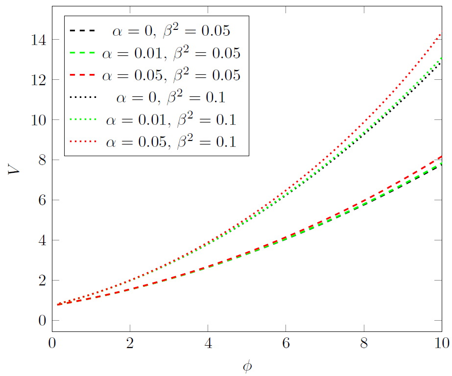
Figure 3: Potential of scalar field for model (26) for the same parameters as on Fig. 2.

For $\gamma=2$ we have the following dependence density of dark energy from scale factor

$$\rho_{d}=\frac{\rho_{d0}}{1-3\beta^{2}\ln a}.$$

The value of $a_{f}=\mathrm{e}^{\beta^{-2}/3}$ corresponds to the moment of final singularity. The energy density tends to infinity for a finite value of the scale factor. With account of thermal radiation, the Universe ends its existence earlier not approaching $a_{f}$. We compared the time for singularity occurrence in this model without thermal radiation and with account of it, in Table 2.

	$w_{0}=-1.05$		$w_{0}=-1.075$		$w_{0}=-1.10$
$\tilde{\alpha}$	$t_{f}-t_{0}$	$t_{0}-t_{a}$	$t_{f}-t_{0}$	$t_{0}-t_{a}$	$t_{f}-t_{0}$	$t_{0}-t_{a}$
0	5.176	0.469	3.432	0.469	2.562	0.469
0.001	5.169	0.465	3.428	0.465	2.558	0.465
0.005	5.140	0.459	3.408	0.459	2.544	0.459
0.01	5.099	0.450	3.381	0.451	2.523	0.451
0.02	5.007	0.434	3.320	0.435	2.477	0.436
0.05	4.680	0.384	3.101	0.387	2.312	0.389

Table 2: Time for singularity $t_{f}-t_{0}$ and time after moment when acceleration began $t_{0}-t_{a}$ in model with thermal radiation (in units of $H_{0}^{-1}$) for $\gamma=2$ in EoS (25). For initial $\Omega_{m}$ the value 0.28 is taken.

For the considered values of $\alpha$, the cosmological evolution in the past does not differ significantly from the model without thermal radiation. The behavior of the parameters $q$ and $j$ for $\gamma=2$ can be seen in Fig. 4.

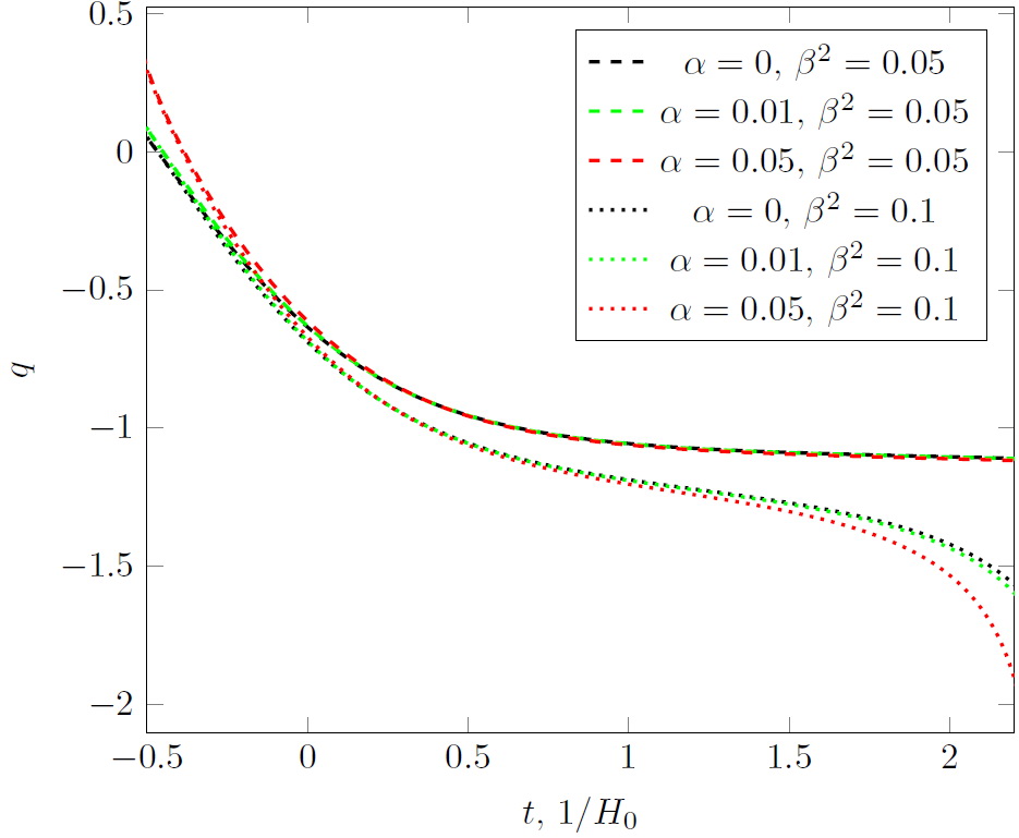
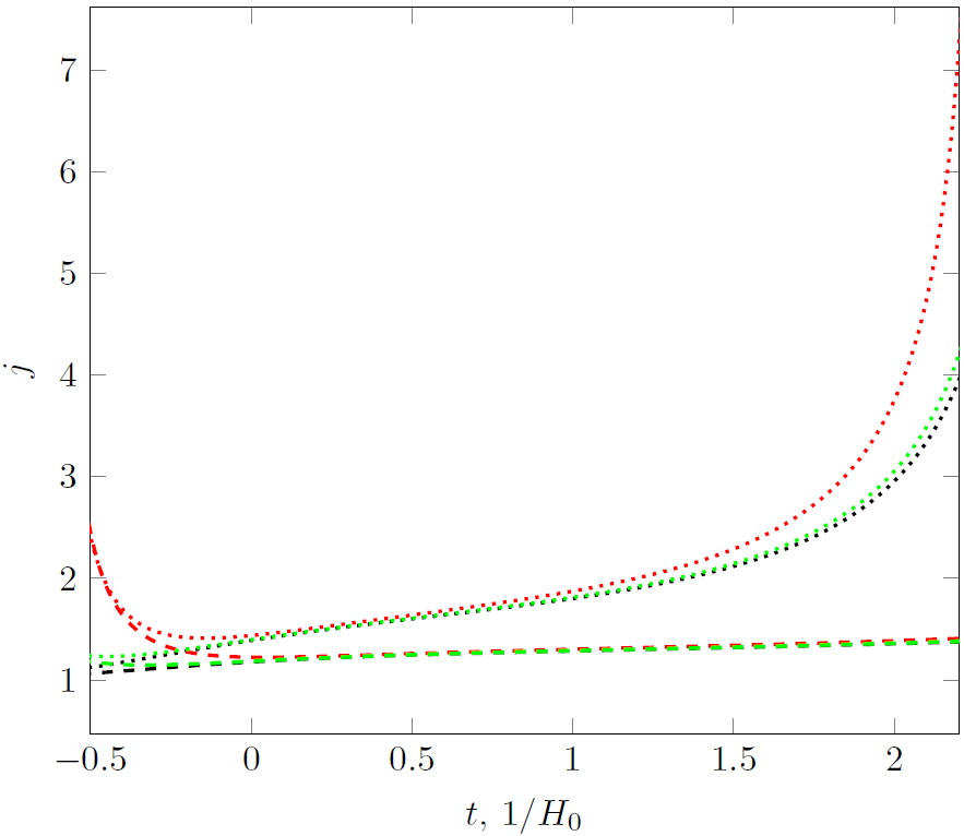
Figure 4: Deceleration (left panel) and jerk (right panel) parameters in model (25) for $\gamma=2$ and some $\beta^{2}$ and $\alpha$. Near the singularity state-finder parameters $q\rightarrow-\infty$, $j\rightarrow\infty$ and its behaviour significantly differs from model without thermal radiation.

V Pseudo-Rip with account of thermal radiation

It is known from the literature that several phantom and quintessence models can lead to the so-called pseudo-Rip singularities Frampton-2 ; Astashenok . The Universe expands asymptotically according to exponential law with some effective “cosmological constant”. It is interesting to investigate influence of thermal radiation on the pseudo-rip expansion of this sort. As an example of such model we shall consider the following,

$$f(\rho_{d})=\pm\beta^{2}\rho_{d0}\frac{\rho_{f}-\rho_{d}}{\rho_{f}-\rho_{d0}},\rho_{f}=\mbox{const}.$$ (34)

We again choose the EoS so that the present time EoS parameter is simply,

$$w_{0}=\frac{p_{d0}}{\rho_{d0}}=-1\mp\beta^{2}.$$

The choice of “+” ($\rho_{f}>\rho_{d0}$) corresponds to phantom model, while the sign “-” ($\rho_{f}<\rho_{d0}$) describes quintessence. For dark energy density as function of scale factor we obtain,

$$\rho_{d}=\rho_{f}-(\rho_{f}-\rho_{d0})a^{-\delta},\quad$$ (35)

$$\delta\equiv\frac{3\beta^{2}\rho_{d0}}{|\rho_{f}-\rho_{d0}|}.$$

If $\rho_{f}<3/4\alpha$ then for large $a$, the energy density tends to $\rho_{f}$, for phantom energy we have that $\rho_{d}\rightarrow\rho_{f}-\epsilon$ while as for quintessence $\rho_{d}\rightarrow\rho_{f}+\epsilon$.

The effective value of ”vacuum energy” due to thermal radiation is larger in comparison to $\rho_{f}$. For $\rho_{f}\rightarrow\frac{3}{4\alpha}$ we have $\rho_{eff}/\rho_{f}\rightarrow 2$. Therefore, the Universe expands faster due to the thermal radiation. The dimensionless parameters $q$ and $h$ behave very similar in both models (see Fig. 5).

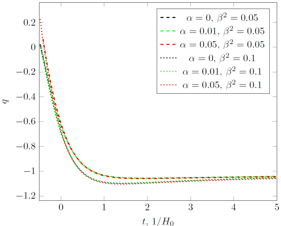
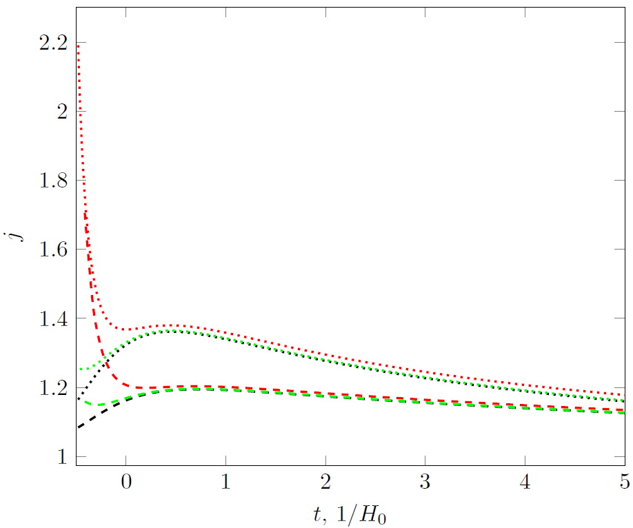
Figure 5: Deceleration (left panel) and jerk (right panel) parameters in model (34) for $\rho_{f}=20$ and some $\beta^{2}$ and $\alpha$.

For $\rho_{f}>3/4\alpha$, a sudden future singularity occurs before exit on quasi-de Sitter expansion.

VI Type II future singularity dark energy

Some models of dark energy can lead to sudden singularity in future without the effect of thermal radiation for example,

$$f(\rho_{d})=\pm\beta^{2}\rho_{d0}\frac{1-\rho_{d0}/\rho_{f}}{1-\rho/\rho_{f}}\,,$$ (36)

If we choose the sign “+”, the energy density increases as the Universe expands (phantom energy). The current EoS parameter $w_{0}$ is simply

$$w_{0}=-1-{\beta^{2}}.$$ (37)

The pressure approaches infinity and a sudden future singularity takes place. For quintessence dark energy, $f(\rho_{d})$ is negative and the final singularity corresponds to $\ddot{a}<0$ (the so-called big crush). Singularity occurs earlier due to the thermal radiation (see Table III).

	$w_{0}=-1.05$		$w_{0}=-1.075$		$w_{0}=-1.10$
$\tilde{\alpha}$	$t_{f}-t_{0}$	$t_{0}-t_{a}$	$t_{f}-t_{0}$	$t_{0}-t_{a}$	$t_{f}-t_{0}$	$t_{0}-t_{a}$
0	41.10	0.470	27.39	0.471	20.53	0.474
0.001	40.99	0.467	27.31	0.468	20.47	0.470
0.005	40.57	0.460	26.99	0.462	20.23	0.464
0.01	39.81	0.452	26.52	0.454	19.88	0.456

Table 3: Time for singularity $t_{f}-t_{0}$ and time after moment when acceleration began $t_{0}-t_{a}$ in model with sudden future singularity (36) (in units of $H_{0}^{-1}$). For initial $\Omega_{m}$ the value 0.28 is taken. Parameter $\rho_{f}$ is 20 (in units of $3H_{0}^{2}$).

For phantom energy density, as function of scale factor, we have the following relation,

$$\rho=\rho_{f}\left(1-\left((1-\Delta)^{2}-6\beta^{2}\Delta(1-\Delta)\ln a\right)^{1/2}\right),\quad\Delta=\rho_{0}/\rho_{f}.$$ (38)

The scale factor in past can be expressed as a function of the redshift, which is defined as,

$$a=\frac{1}{1+z}$$

assuming that the present time scale factor is equal to unity, and the dependence of the luminosity distance $D_{L}$ from the redshift $z$ is

$$D_{L}=\frac{c}{H_{0}}(1+z)\int_{0}^{z}\left(\Omega_{m}(1+z)^{3}+\Omega_{\mathrm{D}}h(z)\right)^{-1/2}dz,$$ (39)

$$h(z)=\Delta^{-1}\left(1-\left(\left(1-\Delta\right)^{2}+6\beta^{2}\ln(1+z)\right)^{1/2}\right).$$

The model under discussion is indistinguishable from the$\Lambda$CDM cosmology for $\Delta<<1$.

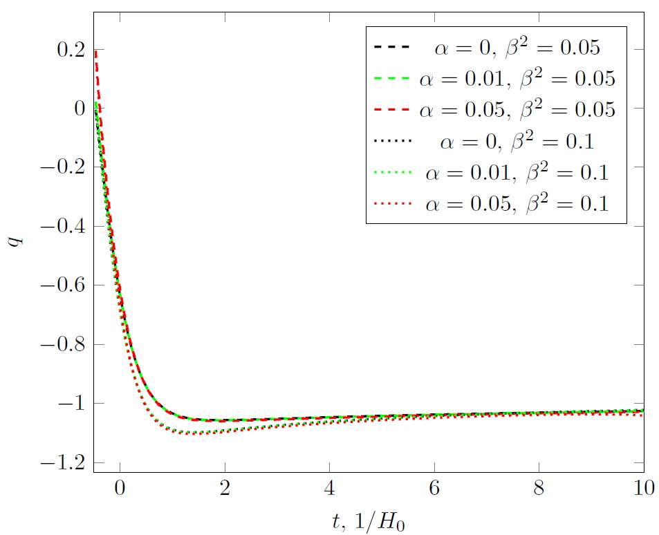
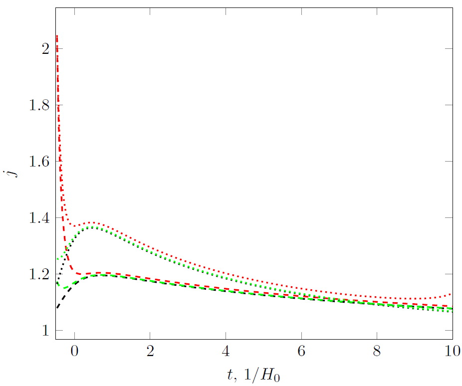
Figure 6: Deceleration (left panel) and jerk (right panel) parameters in model (36) for some $\beta^{2}$ and $\alpha$. Parameter $\rho_{f}$ is 20 (in units of $3H_{0}^{2}$).

The deceleration and jerk parameters are given on Fig. 6 for some values of $\alpha$ and $\beta^{2}$. The example considered above is a good theoretical illustration of dark energy models mimicking vacuum energy, but these models lead to Type II singularities.

VII A Proposal for Evading the Big Rip Chaos: A Dark Fluid Mimicking $R^{2}$ Gravity

In the process of approaching the Big Rip singularity, no matter how this singularity occurs, the Hubble rate grows inevitably, and a cosmological horizon of some sort is expected, as we already discussed in previous sections. One intriguing theoretical question is whether the singularity can be avoided in the first place, if during the dark energy era some term appearing already in the Lagrangian of the theory, makes the singularity milder, or even disappear. In standard modified gravity contexts, such a possibility is realized by adding $R^{2}$ terms in the Lagrangian, see for example Ref. Bamba:2008ut .

Thus it is tempting to add a geometric fluid with EoS parameter of the form $w=w(H,\dot{H},\ddot{H})$ that mimics the $R^{2}$ gravity energy density and pressure, and adding this near a Big Rip singularity. Assuming a flat FRW spacetime, the Friedmann equation near the Big Rip would be at leading order,

$$\frac{3H^{2}}{\kappa^{2}}\simeq\alpha H^{4}+\rho_{\mathcal{G}}\,,$$ (40)

where $\rho_{\mathcal{G}}$ is the $R^{2}$ fluid energy density, the analytic form of which as a function of the Hubble rate and its derivatives with respect to the cosmic time is,

$$\rho_{\mathcal{G}}=-\frac{36\beta H\ddot{H}}{\kappa^{2}}-\frac{108\beta H^{2}\dot{H}}{\kappa^{2}}+\frac{18\beta\dot{H}^{2}}{\kappa^{2}}+\frac{3H^{2}}{\kappa^{2}}\,,$$ (41)

where $\beta$ is a parameter with mass dimensions $[m]^{-2}$. Basically, the energy density $\rho_{\mathcal{G}}$ is essentially the energy density corresponding to an $R^{2}$ geometric fluid of the form $\beta R^{2}$, with the Ricci scalar being as usual $R=12H^{2}+6\dot{H}$ for the flat FRW background. In order to see whether the Big Rip singularity is avoided in the presence of the $R^{2}$ geometric fluid, one must solve the Friedmann equation (40) analytically, which can be cast as follows,

$$\frac{36\beta H\ddot{H}}{\kappa^{2}}+\frac{108\beta H^{2}\dot{H}}{\kappa^{2}}-\frac{18\beta\dot{H}^{2}}{\kappa^{2}}-3\alpha H^{4}\simeq 0\,.$$ (42)

However, this is not an easy task, therefore we shall investigate the behavior of the solutions numerically. We shall adopt the reduced Planck units system, for convenience, in which $\kappa^{2}=1$. The initial time instance of the time loop for our numerical integration will be some initial point when the thermal effects start to occur, so suppose that it is near, $t\sim\mathcal{O}(1/H_{\mathcal{B}})$ where $H_{\mathcal{B}}$ is the value of the Hubble rate when the initial Big Rip singularity is approached, so it is expected to grow significantly near unity in reduced Planck units, in contrast to the tiny present day value in reduced Planck units. So assuming that we run the numerical integration from $t\sim 0.$ in reduced Planck units, which is basically at the beginning of the thermal effects, and by running the numerical integration for $\mathcal{O}(10)$ time units, we obtain the results presented in Fig. 7. Specifically, in Fig. 7 the behavior of the Hubble rate as a function of the cosmic time in reduced Planck units is presented. The time interval is significantly large in reduced Planck units, so this numerical integration actually covers the a large time interval in the far future after the thermal effects started to have a measurable effect in the Friedmann equations. We used various initial conditions for the derivative of the Hubble rate in reduced Planck units, and and for all the plots, the Hubble rate at the beginning of the time loop was assumed to be $H_{\mathcal{B}}\simeq\mathcal{O}(10^{-1})$ and the values of $\alpha$ and $\beta$ where assumed to be of the order of $\alpha,\beta\sim\mathcal{O}(1)$. The red dashed curve corresponds to $\dot{H}(0.)\sim\mathcal{O}(10^{-2})$, the red curve to $\dot{H}(0.)\sim\mathcal{O}(10^{-1})$, while the blue dotted curve to $\dot{H}(0.)\sim\mathcal{O}(10^{-5})$. As it is obvious in all these cases, the Hubble rate grows significantly, but instead of blowing up at finite-time, it reaches a plateau value, which is different for the three different initial conditions, and obviously this is a pure de Sitter state. This final de Sitter approach of the Hubble rate is also common to pure $f(R)$ gravity works, where the $R^{2}$ term eliminates completely the Big Rip singularity from the cosmological evolution Bamba:2008ut ; Nojiri:2008fk ; Capozziello:2009hc . Clearly this result indicates that the $R^{2}$ fluid stabilizes the cosmological evolution, and definitely eliminates the Big Rip singularity. Furthermore, as it was clearly shown in Refs. Bamba:2008ut ; Nojiri:2008fk ; Capozziello:2009hc , in the presence of the $R^{2}$ term or other $f(R)$ gravity models, which yield an exact de Sitter solution at future, apart from the Big Rip singularity, it is also possible to eliminate Type II and III singularities. Hence, the fluid mimicking the $R^{2}$ term in fact eliminates not only Big Rip singularities, but also Type II and Type III singularities, although in principle smooth types of singularities, like the Type IV, can still occur. Furthermore, eventually other fluids which lead to an accelerating Universe, but yield asymptotically de Sitter solutions in the future, also effectively cancel future singularities of Type I,II and III even in presence of thermal effects.

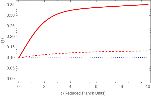
Figure 7: The Hubble rate as a function of the cosmic time in reduced Planck units, in the presence of an $R^{2}$ fluid. The final de Sitter point is reached and the Big Rip singularity is avoided, for various distinct initial conditions of $\dot{H}$, at the moment that the thermal effects affect the evolution.

VIII Conclusion

In this work we considered dark energy models by taking into account thermal radiation effects. We assumed that this radiation contributes to the total energy density with a energy density term which is proportional to $H^{4}$, where $H$ is the Hubble rate. Consequently, if the dark energy density values grow infinitely as the Universe expands (phantom energy), then we can be certain that a sudden future singularity takes place, or is approached inevitably in the near future. For some finite energy density $\rho_{m}$ and scale factor, the second derivative of scale factor diverges. Thermal radiation leads to the so-called little rip scenario, when the dark energy density increases infinitely with time and the EoS parameter approaches the value $-1$ asymptotically at $t\rightarrow\infty$. The cosmological expansion with a future Big Rip, without thermal radiation, also changes to an evolution leading to a sudden singularity. It is interesting to note that the phase of accelerated expansion in models with thermal radiation, begins later in comparison with cosmological models without this contribution, but the final singularity takes place earlier.

The realization of a quasi-de Sitter expansion (pseudo-rip) depends on the dark energy EoS. If the EoS parameter for dark energy develops a zero value at some density $\rho_{f}$, then if $\rho_{f}>\rho_{m}$, the sudden singularity still occurs. In the opposite case the Universe evolves to a de Sitter regime with some effective “cosmological constant”, larger in comparison with $\rho_{f}$. For $\rho_{f}$ close to $\rho_{m}$ we have $\rho_{eff}/\rho_{f}\rightarrow 2$. In effect, the Universe expands faster and evolves to the de Sitter expansion earlier. In the case of an EoS with singularity (pressure tends to $\infty$ at some finite $\rho_{f}$) we have in any case a sudden future singularity. The inclusion of thermal radiation does not make worse the compliance of the cosmological models with the observational data. One can construct (as we have here) models that mimic the standard $\Lambda$CDM model up to present time, but the contribution of the thermal radiation can switch the future cosmological evolution to a regime with a sudden future singularity.

At present time, dark energy remains a mystery and quite many questions related to it are still not answered concretely. The current models describing dark energy only answer some questions, but to date no definitive answer is given. The main model which remains with good compliance with the observational data is the $\Lambda$CDM model, and thus many dark energy models originating from various theoretical contexts, are mainly designed to mimic the $\Lambda$CDM model. But the $\Lambda$CDM model has its weak points, two of which already appear in its name, $\Lambda$ and Cold Dark Matter. With regards to the latter, dark matter is a speculation, but no dark matter particle has ever been observed. With regard to $\Lambda$, the cosmological constant, its nature is unknown, and if it is seen as the vacuum energy, its present day value is extremely small and infinitely smaller from the predicted vacuum energy value from quantum field theories. Apart from these two, there exist other conceptual issues to be resolved in the future, such as if the dark energy itself is dynamical or not, and more importantly, is the dark energy era a phantom dark era? If one sticks on the general relativistic approach and insist on using he general relativistic recipe to describe the dark energy era, so the usage of $\Lambda$ or scalar fields, the last two questions will probably make their presence in a predominant way. This is because in the case of dynamical dark energy with a varying EoS, the cosmological constant would not fit at all, since it yields a constant de Sitter EoS. Regarding the phantom question, things are getting worse if one sticks with the general relativistic recipe, scalar fields, since phantom scalar fields must be used and phantom scalar fields from a theoretical point of view are instabilities. Nevertheless, even if one adopts the phantom scalar field description for the phantom dark energy era, the result would be a Big Rip singularity as was demonstrated in Ref. Caldwell-2003 . Thus the study of future finite-time singularities is a possible eschatological scenario of our Universe. In view of these questions, modified gravity in its various forms, stands on a promising solid ground, since it answers in a relatively successful way many of these questions. In the models we presented in this work, we were able to generate phantom evolution without the need for phantom scalar fields, and we also indicated that finite-time singularities can actually occur by using various fluid approaches, without again the need for phantom fluids, like for example in general relativistic contexts. In addition, some of the models can mimic at present-time the $\Lambda$CDM model, and also can provide a viable present day dark energy era, compatible with the Planck data. In addition, we discussed how the evolution would change if we took into account the thermal effects, thus our model indicates a road map towards possible future evolutions. Of course our approach is one of the many possible scenarios, however the future observations are promising, thus as theorists we try to investigate all the possible scenarios.

References

- (1) A. G. Riess et al., Astron. J. 116, 1009 (1998).
- (2) S. Perlmutter et al., Ap. J. 517, 565 (1999).
- (3) K. Bamba, S. Capozziello, S. Nojiri and S. D. Odintsov, Astrophys. Space Sci. 342 (2012), 155-228 doi:10.1007/s10509-012-1181-8 [arXiv:1205.3421 [gr-qc]].
- (4) M. Li, X. Li, S. Wang and Y. Wang, Commun. Theor. Phys. 56, 525 (2011).
- (5) Y. -F. Cai, E. N. Saridakis, M. R. Setare and J. -Q. Xia, Phys. Rept. 493 (2010) 1 [arXiv:0909.2776 [hep-th]].
- (6) Y. Akrami et al. [Planck Collaboration], arXiv:1807.06211 [astro-ph.CO].
- (7) M. Kowalski, Ap. J. 686, 74 (2008).
- (8) K. Nakamura et al. [Particle Data Group Collaboration], J. Phys. G G 37, 075021 (2010).
- (9) R. Amanullah et al., Ap. J. 716, 712 (2010).
- (10) R. R. Caldwell, Phys. Lett. B 545 23 (2002).
- (11) R. R. Caldwell, M. Kamionkowski and N. N. Weinberg, Phys. Rev. Lett. 91, 071301 (2003).
- (12) S. M. Carroll, M. Hoffman and M. Trodden, Phys. Rev. D68, 023509 (2003).
- (13) S. Nesseris and L. Perivolaropoulos, JCAP 0701 (2007) 018 [astro-ph/0610092].
- (14) P. H. Frampton and T. Takahashi, Phys. Lett. B 557, 135 (2003).
- (15) S. Nojiri and S. D. Odintsov, Phys. Lett. B 562, 147 (2003) [arXiv:hep-th/0303117].
- (16) V. Faraoni, Int. J. Mod. Phys. D 11, 471 (2002) [arXiv:astro-ph/0110067].
- (17) P. F. Gonzalez-Diaz, Phys. Lett. B 586, 1 (2004) [arXiv:astro-ph/0312579].
- (18) E. Elizalde, S. Nojiri and S. D. Odintsov, Phys. Rev. D 70, 043539 (2004) [arXiv:hep-th/0405034].
- (19) P. Singh, M. Sami and N. Dadhich, Phys. Rev. D 68, 023522 (2003) [arXiv:hep-th/0305110].
- (20) C. Csaki, N. Kaloper and J. Terning, Annals Phys. 317, 410 (2005) [arXiv:astro-ph/0409596].
- (21) P. X. Wu and H. W. Yu, Nucl. Phys. B 727, 355 (2005) [arXiv:astro-ph/0407424].
- (22) S. Nesseris and L. Perivolaropoulos, Phys. Rev. D 70, 123529 (2004) [arXiv:astro-ph/0410309].
- (23) H. Stefancic, Phys. Lett. B 586, 5 (2004) [arXiv:astro-ph/0310904].
- (24) L. P. Chimento and R. Lazkoz, Phys. Rev. Lett. 91, 211301 (2003) [arXiv:gr-qc/0307111].
- (25) J. G. Hao and X. Z. Li, Phys. Lett. B 606, 7 (2005) [arXiv:astro-ph/0404154].
- (26) M. P. Dabrowski and T. Stachowiak, Annals Phys. 321, 771 (2006) [arXiv:hep-th/0411199].
- (27) S. Nojiri and S. D. Odintsov, Phys. Rev. D 70 (2004) 103522 [hep-th/0408170].
- (28) J. Barrow, Class. Quant. Grav. 21, L79 (2004).
- (29) Y. Shtanov and V. Sahni, Class. Quant. Grav. 19 (2002) L101 [gr-qc/0204040].
- (30) S. Nojiri and S. D. Odintsov, Phys. Lett. B 595, 1 (2004) [arXiv:hep-th/0405078].
- (31) S. Cotsakis and I. Klaoudatou, J. Geom. Phys. 55, 306 (2005) [arXiv:gr-qc/0409022].
- (32) M. P. Dabrowski, Phys. Rev. D 71, 103505 (2005) [arXiv:gr-qc/0410033].
- (33) L. Fernandez-Jambrina and R. Lazkoz, Phys. Rev. D 70, 121503(R) (2004) [arXiv:gr-qc/0410124].
- (34) Phys. Lett. B 670, 254 (2009) [arXiv:0805.2284 [gr-qc]].
- (35) J. D. Barrow and C. G. Tsagas, Class. Quant. Grav. 22, 1563 (2005) [arXiv:gr-qc/0411045].
- (36) H. Stefancic, Phys. Rev. D 71, 084024 (2005) [arXiv:astro-ph/0411630].
- (37) C. Cattoen and M. Visser, Class. Quant. Grav. 22, 4913 (2005) [arXiv:gr-qc/0508045].
- (38) P. Tretyakov, A. Toporensky, Y. Shtanov and V. Sahni, Class. Quant. Grav. 23, 3259 (2006) [arXiv:gr-qc/0510104].
- (39) A. Balcerzak and M. P. Dabrowski, Phys. Rev. D 73, 101301(R) (2006) [arXiv:hep-th/0604034].
- (40) A. V. Yurov, A. V. Astashenok and P. F. Gonzalez-Diaz, Grav. Cosmol. 14, 205 (2008) [arXiv:0705.4108 [astro-ph]].
- (41) J. D. Barrow and S. Z. W. Lip, Phys. Rev. D 80, 043518 (2009) [arXiv:0901.1626 [gr-qc]].
- (42) M. Bouhmadi-Lopez, Y. Tavakoli and P. V. Moniz, JCAP 1004, 016 (2010) [arXiv:0911.1428 [gr-qc]].
- (43) P. H. Frampton, K. J. Ludwick and R. J. Scherrer, Phys. Rev. D 84 (2011) 063003 [arXiv:1106.4996 [astro-ph.CO]].
- (44) P. H. Frampton, K. J. Ludwick and R. J. Scherrer, arXiv:1112.2964 [astro-ph.CO].
- (45) P. H. Frampton, K. J. Ludwick, S. Nojiri, S. D. Odintsov and R. J. Scherrer, Phys. Lett. B 708 (2012) 204 [arXiv:1108.0067 [hep-th]].
- (46) A. V. Astashenok, S. Nojiri, S. D. Odintsov and A. V. Yurov, arXiv:1201.4056 [gr-qc].
- (47) G. W. Gibbons and S. W. Hawking, Phys. Rev. D 15 (1977) 2738.
- (48) R. G. Cai, L. M. Cao and Y. P. Hu, Class. Quant. Grav. 26 (2009).
- (49) R. Ruggiero, [arXiv:2005.12684 [gr-qc]].
- (50) S. Nojiri and S. D. Odintsov, Phys. Dark Univ. 30 (2020) 100695 [arXiv:2006.03946 [gr-qc]].
-
(51)
S. Nojiri, S. D. Odintsov and S. Tsujikawa,
Phys. Rev. D 71 (2005) 063004
[hep-th/0501025];
S. Nojiri and S. D. Odintsov, Phys. Rev. D 72 (2005) 023003 [hep-th/0505215]. - (52) R. Amanullah, C. Lidman, D. Rubin, G. Aldering, P. Astier, K. Barbary, M. S. Burns and A. Conley et al., Astrophys. J. 716, 712 (2010) [arXiv:1004.1711 [astro-ph.CO]].
- (53) V. Sahni, T. D. Saini, A. A. Starobinsky and U. Alam, JETP Lett. 77 (2003) 201 [Pisma Zh. Eksp. Teor. Fiz. 77 (2003) 249] [astro-ph/0201498].
- (54) K. Bamba, S. Nojiri and S. D. Odintsov, JCAP 10 (2008), 045 doi:10.1088/1475-7516/2008/10/045 [arXiv:0807.2575 [hep-th]].
- (55) S. Nojiri and S. D. Odintsov, Phys. Rev. D 78 (2008) 046006 doi:10.1103/PhysRevD.78.046006 [arXiv:0804.3519 [hep-th]].
- (56) S. Capozziello, M. De Laurentis, S. Nojiri and S. D. Odintsov, Phys. Rev. D 79 (2009) 124007 doi:10.1103/PhysRevD.79.124007 [arXiv:0903.2753 [hep-th]].