Percolation perspective on sites not visited by a random walk in two dimensions

Abstract

We consider the percolation problem of sites on an $L\times L$ square lattice with periodic boundary conditions which were unvisited by a random walk of $N=uL^{2}$ steps, i.e., are vacant. Most of the results are obtained from numerical simulations. Unlike its higher-dimensional counterparts, this problem has no sharp percolation threshold and the spanning (percolation) probability is a smooth function monotonically decreasing with $u$. The clusters of vacant sites are not fractal but have fractal boundaries of dimension 4/3. The lattice size $L$ is the only large length scale in this problem. The typical mass (number of sites $s$) in the largest cluster is proportional to $L^{2}$, and the mean mass of the remaining (smaller) clusters is also proportional to $L^{2}$. The normalized (per site) density $n_{s}$ of clusters of size (mass) $s$ is proportional to $s^{-\tau}$, while the volume fraction $P_{k}$ occupied by the $k$th largest cluster scales as $k^{-q}$. We put forward a heuristic argument that $\tau=2$ and $q=1$. However, the numerically measured values are $\tau\approx 1.83$ and $q\approx 1.20$. We suggest that these are effective exponents that drift towards their asymptotic values with increasing $L$ as slowly as $1/\ln L$ approaches zero.

I Introduction

Percolation theory Stauffer and Aharony (1991); Gremmett (1999); Saberi (2015) provides a statistical description of long-range connectivity in lattices or networks when some of their sites or links have been removed. First emerging in the context of polymer sciences Flory (1941); Stockmayer (1944) and spread of a fluid through a porous medium Broadbent and Hammersley (1957), this theory remains a very active field of research with very diverse applications, ranging from topography Saberi (2013), epidemiology Grassberger (1983); Matamalas et al. (2018), gelation and colloid science Anekal et al. (2006); Coniglio et al. (1979); Tsurusawa et al. (2019); Adam et al. (1990), environmental Taubert et al. (2018) and urban Makse et al. (1995) studies, through more abstract networks Havlin et al. (2015); Kalisky and Cohen (2006); Derényi et al. (2005); Callaway et al. (2000) and more Saberi (2015). In this paper we consider a two-dimensional case of a variant of the percolation problem, where an initially full lattice has its sites removed by a single meandering random walk (RW). The three-dimensional version of the problem models a degradation of a gel by a single enzyme, or very few enzymes, that break the crosslinks they encounter Berry et al. (2000); Fadda et al. (2003).

A percolating system can be characterized by the level of its occupation, such as the fraction $p$ of sites present on the lattice, or the occupied volume fraction in a continuous system. (In this paper we consider site percolation on hypercubic lattices, but the results equally well apply to lattice bonds or mixed site-bond problems and other types of lattices.) In the case of lattice percolation the geometry can be viewed as a collection of clusters formed by neighboring (“connected”) occupied sites. A cluster is spanning if it forms a continuous path between opposing boundaries in a specific direction. For an infinite system, the emergence of a spanning cluster can be characterized as a phase transition: there exists a sharp percolation threshold $p_{c}$, such that for $p>p_{c}$ there exists an infinite spanning cluster. Both above and below $p_{c}$ the mean spatial extent (linear size) of finite clusters is called correlation length $\xi$. It diverges near the threshold as $\xi\sim|p-p_{c}|^{-\nu}$, where the universal exponent $\nu$ is independent of microscopic details of the model, but does depend on the dimensionality $d$ of the system and, possibly, the presence of long-range correlations. The universality of the critical exponents allows application of the results of simple models to more realistic and complicated cases.

One of the simpler percolation models is Bernoulli site percolation on a $d$-dimensional lattice where each lattice site is independently occupied with probability $p$. The exponent $\nu$ of the Bernoulli problem decreases from $\nu_{B}=1$ at the lower critical dimension $d=1$ to $\nu_{B}=1/2$ for $d\geq d_{c}=6$, i.e., at and above the upper critical dimension $d_{c}$ Toulouse (1974). The generalized Harris criterion Harris (1974) has been used to show Weinrib (1984) that percolation models with short-range correlations or with power-law correlations $\sim 1/r^{b}$ with large power $b$ also belong to the Bernoulli percolation universality class. However, if $b<2/\nu_{\rm B}$, then the correlations are relevant, and $\nu=2/b$ Weinrib (1984). There is a variety of studies of correlated percolation Coniglio and Fierro (2009); Gori et al. (2017); Riordan and Warnke (2011); D’Souza and Nagler (2015); Kantor (1986).

In space dimension $d$ we can consider an initially full hypercubic lattice of linear size $L$ (in lattice constants) and number of sites $M=L^{d}$ the sites of which are being removed by an $N$-step RW that started at a random position. Periodic boundary conditions are imposed, i.e., the walker exiting through one boundary of the lattice reemerges on the opposite boundary. The number of steps $N$ of the walker is proportional to the volume of the system, i.e., $N=uL^{d}$, with parameter $u$ controlling the length of the walk. In the case of gel of crosslinked polymers the random walker represents an enzyme that breaks the crosslinks of a gel that it encounters Berry et al. (2000); Fadda et al. (2003). The object of the study are the vacant sites not visited by the random walker, that represent the surviving crosslinks. The variable $u$ controls the concentration of vacant sites and naturally replaces $p$ used in the regular percolation. For $3\leq d\leq 6$ infinite clusters of vacant sites appear for $u$ below similar threshold values $u_{c}\approx 3$ Kantor and Kardar (2019). Banavar et al. studied the geometry of the clusters created by the vacant sites in $d=2$ and $3$ Banavar et al. (1985), while Abete et al. considered the critical behavior near the percolation threshold in $d=3$ Abete et al. (2004). More recently Kantor and Kardar studied the percolation properties of the problem for $2\leq d\leq 6$ Kantor and Kardar (2019).

Sites visited by an $N$-step RW on an infinite lattice are strongly correlated. The final position of such a walk is at a distance $r\approx aN^{1/2}$ away from its starting point, where $a$ is the lattice constant. This means that number of steps (“mass”) scales as $N\sim r^{2}$, and the fractal dimension Mandelbrot (1982) of a RW is $d_{f}=2$ independently of the embedding dimension $d$. Therefore, we may expect our problem to behave differently in $d=2$ than at higher $d$. A RW can traverse a finite lattice of linear size $L$ in $\sim L^{2}$ steps, and therefore a walk of $uL^{d}$ steps traverses (“crosses”) the lattice

$${\cal N}_{\rm cr}\approx uL^{d-2}$$ (1)

times. For $d\geq 3$ the increase in lattice size $L$ increases ${\cal N}_{\rm cr}$, while a strand of RW on every single “crossing” leaves sparser “footprints” on the lattice. (The total density of visited or vacant sites in $d\geq 3$ remains independent of $L$ and depends only on $u$.) This makes the “thermodynamic limits” somewhat peculiar even for $d\geq 3$ since with the increase of $L$, the structure of the system changes, rather than having more similar pieces being added to it.

On an infinite lattice the density of sites visited by an $N$-step RW (for $d\geq 3$) within the distance visited by the walk is $N/r^{d}\sim 1/r^{d-2}$. On a finite lattice, the sites belonging to different strands of RW created due to periodicity of the lattice are almost uncorrelated. The repeated crossings only contribute to the uncorrelated density of sites. However, the correlation is preserved for $r$ smaller than the lattice size for sites situated on the same strand of the RW. Consequently, the cumulant of the correlation (from which the overall background density has been subtracted) has the same power-law relation. Consider a random variable $v(\vec{x})$ which is 1 if the site at position $\vec{x}$ is vacant, and zero otherwise. It is complementary to the variable representing the visited site (their sum is 1) and therefore, it has the same cumulant: $\langle v(\vec{x})v(\vec{y})\rangle_{c}\sim 1/|\vec{x}-\vec{y}|^{d-2}$ Kantor and Kardar (2019). Thus, for correlation power $b=d-2$, the correlation length exponent $\nu=2/b$ Weinrib (1984) becomes

$$\nu=2/(d-2),\ \ {\rm for}\ \ 3\leq d\leq 6.$$ (2)

The ubiquitous factor “$d-2$” appearing in the above discussions, such as in Eqs. (1) and (2), or expressions for the correlation functions, indicates that many of the arguments presented for $d\geq 3$ will change in the two-dimensional case. In this paper we focus on the vacant site properties in $d=2$ from the point of view of percolation theory. Despite the absence of percolation threshold, the system has many scaling properties that resemble critical phenomena. In Sec. II we point out the unusual features of $d=2$, and begin a discussion of two-dimensional vacant site (unvisited by a RW) percolation (2DVSP) at a point where Ref. Kantor and Kardar (2019) left off. Furthermore, in Sec. II we explain the main properties that set 2DVSP apart from vacant site percolation in higher dimensions and verify the absence of a sharp percolation threshold in $d=2$. In Sec. III we consider the mean sizes of the largest cluster and other clusters, and demonstrate the role played by the lattice size $L$ in the description of the system. Our results show that $L$ is the main length scale of the problem, which replaces the correlation length $\xi$ of other percolation problems. In particular, we show that the spanning cluster volume and the mean volume of finite clusters both scale as $L^{2}$. In Sec. IV we focus on the geometry of the spanning cluster and demonstrate that the large clusters in $d=2$ are not fractal, contrary to the results of the previous study Banavar et al. (1985). Nevertheless, we show that the boundaries of those clusters are fractal with dimension 4/3. In Sec. V we study in detail the cluster statistics in 2DVSP. We put forward a heuristic argument describing cluster statistics and the effective exponents measured numerically are close to the proposed theoretical values. We summarize and point out directions of future research in Sec. VI.

II How special is $d=2$?

(a)

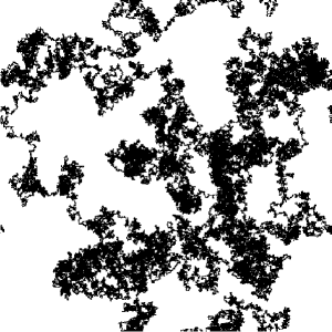
(b)

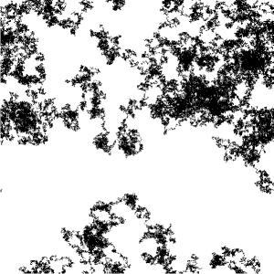
(c)

Figure 1: Examples of random walks (black) of $N=uL^{2}$ steps ($u=1.3$) on a periodic square lattice of size $L^{2}$ for (a) $L=64$, (b) 512, and (c) 4096. Despite having the same RW length parameter $u$, the actual fraction of the vacant (unvisited) white sites increases with $L$ from (a) $p=0.60$ to (b) 0.70 and to (c) 0.78.

Since the fractal dimension of RW is 2, it “almost” fills the two-dimensional embedding space: in $d=2$ the number of distinct sites visited by an $N$-step RW on an infinite square lattice increases for long walks as $N_{\rm dist}=\pi N/\ln{N}$ Dvoretzky and Erdős (1951), i.e., slightly slower than $N$, because the walk is recurrent and keeps revisiting previously visited sites an ever increasing number of times. (In contrast, at $d\geq 3$ the number of distinct visited sites is asymptotically proportional to $N$ Vineyard (1963); Rubin and Weiss (1982) since the number of repeated visits approaches a constant Pólya (1921); Hughes (1995).) The presence of the logarithmic correction in $N_{\rm dist}$ has consequences for a RW of $N=uL^{2}$ steps on a finite square lattice of linear size $L$ ($0\leq$$x_{1},x_{2}$$\leq L-1$) and volume $M=L^{2}$. We assume periodic boundary conditions in both directions, i.e., the coordinate $x_{i}=L$ coincides with $x_{i}=0$ for $i=1,2$. On such a lattice, it has been proven Brummelhuis and Hilhorst (1992) (see also Ref. Kantor and Kardar (2019)) that the mean fraction of unvisited (vacant) sites for large $L$ is

$$p=\exp{\left(-\frac{\pi u}{2\ln{L}}\right)}\,.$$ (3)

(For a finite square lattice of $M$ sites, a RW needs on the average $\frac{1}{\pi}M\ln^{2}M$ steps to visit all the sites of the lattice Aldous (1983); Nemirovsky et al. (1990); Brummelhuis and Hilhorst (1991); Dembo et al. (2004); Mendonça (2011); Grassberger (2017). The area of complete or nearly complete coverage Brummelhuis and Hilhorst (1992); Dembo et al. (2006); Comets et al. (2013) of a lattice, exhibits unusual effects of discreetness, such as correlations between unvisited points, and has been extensively studied. If one just concentrates on the density of unvisited sites and disregards their connectivity or clusters, it is possible to identify a fractal behavior with a power-law that depends on the extent to coverage. However, this limit corresponds to $u=\infty$ in our problem, while we are concerned only with finite $u$s.)

In Eq. (3) the fraction $p$ of vacant sites depends on $L$ and it deprives us of a simple correspondence between $p$ and $u$, which is present in $d\geq 3$, where $p=\exp(-A_{d}u)$ with some constant $A_{d}$ Brummelhuis and Hilhorst (1991); Kantor and Kardar (2019). However, we note that for fixed $u$ in $d=2$ in the $L\to\infty$ limit, we have $p\to 1$. Figure 1 depicts RWs with the same $u$ for three different $L$s, demonstrating the tendency of increasing $p$ with increasing $L$. For very large $L$s we can treat the clusters of vacant sites as being separated by “thin regions” of RWs. [The results in Fig. 1 as well as in many following figures are presented for $u=1.3$. They do not differ qualitatively from any other $u=O(1)$. The convenience of showing the data for this particular value of $u$ is explained later in this section and in Sec. IV.] Since Eq. (3) is valid only asymptotically for large $L$, we measured numerically the mean fraction of vacant sites $p$ for fixed $u=1.3$ and increasing $L$. The results are depicted in the semilogarithmic plot in Fig. 2, and at such scale Eq. (3) should be represented by a straight line. We see that Eq. (3) is satisfied already for $L\sim 100$. However, the limit of $p=1$ is approached slowly: for large $L$ the dependence is $p\approx 1-\pi u/2\ln{L}+\dots$. Even for $L=512$ and $u=1.3$, the fraction of vacant sites $p\approx 0.72$, while for $L=10^{6}$ we only have $p\approx 0.86$, and the regime of $p\approx 1$ is numerically inaccessible to us.

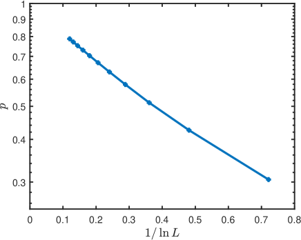
Figure 2: Semilogarithmic plot of numerically measured fraction $p$ of vacant sites for $u=1.3$ as a function of $1/\ln L$, for $L$ ranging between 4 and 4096. (Statistical errors in $p$ calculated from $3\cdot 10^{5}$ configurations are smaller than the symbol sizes.) Fraction $p\to 1$ as $(1/\ln L)\to 0$, as predicted by Eq. (3).

When Bernoulli percolation is formulated on, say, a $d$-dimensional hypercubic lattice, the dimensionless percolation threshold $p_{c}$ is reached when a sufficient number of sites is added to an empty lattice or a sufficient number is removed from a full lattice. In continuum percolation this corresponds to a finite fraction of the system volume being occupied or removed. When a percolating situation is created by a RW removing parts of the system, we may separately consider the length $\ell$ of the single step of the RW and the volume $a^{d}$ occupied by a certain position $\vec{r}_{i}$ of the step of the RW. On a lattice the “size” of the site $a$ and the length $\ell$ of the step are both assumed to be equal to the lattice constant. Thus, at any $d$ a short $N$-step RW occupies a volume proportional to $Na^{d}$ on a lattice of volume $(aL)^{d}$. If the RW performs $N=uL^{d}$ steps, then in $d\geq 3$ the fraction of vacant sites is $p=\exp(-A_{d}u)$. This means that for $d\geq 3$ there should exist a critical value $u_{c}$. This has been proven theoretically Dembo and Sznitman (2006); Benjamini and Sznitman (2008); Sznitman (2008); Sidoravicius and Sznitman (2009); Sznitman (2010); Černý et al. (2011); Balázs (2015) and demonstrated numerically Kantor and Kardar (2019). (Approaches used in some of these works also implied the absence of threshold in $d=2$.)

It has been mentioned in Sec. I that for $d\geq 3$ the increase of $L$ for fixed $u$ causes the increase in lattice crossings by the RW as expected from the $L$ dependence of ${\cal N}_{\rm cr}$ in Eq. (1). In $d=2$ the situation is very different: on one hand, the value of $u$ no longer solely determines the fraction of occupied or vacant sites due to $L$ dependence in Eq. (3). On the other hand, the number of lattice crossings by the RW only depends on $u$ and not on the lattice size $L$. The probability of having a spanning cluster in, say, vertical direction depends on the ability of the RW to create a continuous path blocking vertical connection and is independent of the two-dimensional “volume” occupied by the RW. In the absence of a lattice the presence of a “blocking path” will depend on the typical step size $\ell$ of the RW rather than volume (area) $a^{2}$ occupied by each position.

Numerically, we consider site percolation on a periodic square lattice of $L^{2}$ sites. A random walker starts at an arbitrary site and performs $N=uL^{2}$ steps with $u=O(1)$. If there is a continuous path of vacant sites (unvisited by the RW) that connects the top and bottom boundaries $x_{2}=0$ and $L-1$, we say that the configuration is spanning (percolating). Figure 3 depicts the spanning probability $\Pi$ as a function of $u$, for lattice sizes $L$ ranging from $4$ to $512$. (The steps visible on the graph for $L=4$ are a result of truncating $uL^{2}=16u$ to an integer.) We see that the graphs of $\Pi(L,u)$ converge as $L$ increases with the limit being a smooth function $\Pi(\infty,u)$, thus indicating that there is no percolation threshold. (The graphs in Fig. 3 are similar to the results in Ref. Kantor and Kardar (2019).) This differs from systems with a sharp percolation threshold such as vacant site percolation in $d\geq 3$ or Bernoulli percolation, where for $L\gg\xi$, $\Pi$ rapidly decreases from $1$ to $0$ around the percolation threshold and becomes a step function in the $L\to\infty$ limit.

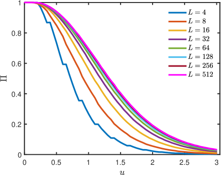
Figure 3: Percolation probability $\Pi(L,u)$ for $L=4,8,\dots,512$ (bottom left to top right). Each point is an average of $5\cdot 10^{5}$ configurations and the points are separated by $\Delta u=0.05$.

The continuous curve in Fig. 3 demonstrates the absence of a transition in $d=2$. Due to the central limit theorem, very long lattice RWs Rudnick and Gaspari (2004) can, on a coarse-grained level, be treated as Gaussian RWs in continuous space Hughes (1995) when the probability of a particular configuration $\{\vec{r}_{i}\}$ of step positions of an $N=uL^{2}$ step walk is proportional to $\exp\left[-\sum_{i=1}^{N}(\vec{r}_{i}-\vec{r}_{i-1})^{2}/\ell^{2}\right]$. (Corrections to Gaussian behavior are irrelevant in the renormalization group sense and their relative strength decays upon repeated coarse-graining Amit (1993).) The decrease of $L$ by, say, a factor $\lambda$, and $N$ by a factor $\lambda^{2}$, is equivalent to simply integrating out $\lambda^{2}-1$ out of every $\lambda^{2}$ variables $\vec{r}_{i}$ (decimation), which leads to the same functional shape of the probability with a simple replacement of $\ell$ by $\lambda\ell$ without any change of the system volume. Thus, the Gaussian RW is exactly coarse-grained without changing the overall distances between points. Not surprisingly, such an operation usually does not change the spanning cluster, except for slight coarse-graining of its boundaries. (The “exact” nature of coarse-graining transformation applies only to the distances, but may have nontrivial topological issues, such as breaking apart of a spanning cluster which was weakly connected before the transformation, or joining of two nearby clusters and creating a spanning cluster. While such events are unlikely, they render the entire argument inexact. An example of topological issues of RWs can be found in the problem of a winding number - see Ref. Drossel and Kardar (1996) and references therein.) The above argument can equally well be used in the opposite direction for fine-graining the system by a factor $\lambda$, which involves a replacement of every bond of a Gaussian RW, by $\lambda^{2}$ shorter steps with $\ell$ replaced by $\ell/\lambda$. This fine-graining corresponds to an increase of overall system size from $L$ to $\lambda L$. The $L$ dependence visible in Fig. 3 for $L\lesssim 100$ is a consequence of the transition from a RW on a discrete lattice to an essentially continuous Gaussian RW behavior. Examination of the $L$ dependence of $\Pi$ for a fixed $u$ shows that the curves in Fig. 3 almost reached their asymptotic values.

We can interpret the spanning probability $\Pi$ as an average of a random variable $\Pi^{\prime}(N)$ which has the value $1$ when there is a spanning cluster and zero otherwise, when an $N$-step walk has been generated. For a specific realization of a RW the variable $\Pi^{\prime}=1$ as the walk begins, and at some step $N_{0}$ the RW disconnects the spanning cluster, and the system no longer percolates, i.e., $\Pi^{\prime}=0$ for $N\geq N_{0}$. The “discrete derivative” of this function is $\frac{\Delta\Pi^{\prime}}{\Delta N}=-\delta_{NN_{0}}$, where $\delta_{ij}$ is the Kronecker delta. For large $L$, this can be written in terms of the continuous variable $u$ as $\frac{d\Pi^{\prime}}{du}=-\delta(u-u_{0})$, where $\delta(x)$ is the Dirac delta-function and the percolation stops after exactly $u_{0}L^{2}$ steps for that configuration. Clearly, the ensemble averaging over all possible RWs corresponding to a given $u$ results in the equality $\left|\frac{d\Pi}{du}\right|=-\left\langle\frac{d\Pi^{\prime}}{du}\right\rangle=\left\langle\delta(u-u_{0})\right\rangle$, which is exactly the probability distribution of the percolation stopping times $u_{0}$. Calculating $\left|\frac{d\Pi}{du}\right|$ from the data in Fig. 3, we find that for large $L$s the distribution of percolation stopping times converges to a broad peak centered around $u=u^{*}=1.3$ with half-width of approximately $0.8$. For every RW, one step before the span breaking number $N_{0}$ is reached, the spanning cluster contains at least one “bottleneck” that will be pinched off at the next step. Thus, the derivative $d\Pi/du$ can also be viewed as characterizing such situations.

All the special features of the 2DVSP problem described in this section qualify $d=2$ to be called the lower critical dimension of the vacant site percolation problem. However, it qualitatively differs from the lower critical dimension of Bernoulli percolation Stauffer and Aharony (1991). For the latter, $d=1$ is the lower critical dimension with a trivial percolation threshold ($p_{c}=1$) and various properties that can be calculated analytically. Besides being a relatively simple problem, Bernoulli percolation for $p<1$ in $d=1$ has a finite correlation length $\xi$ that simply depends on $p$, and the system becomes homogeneous beyond that length scale. We shall see that 2DVSP does not have such a length scale, and its structure keeps changing with the increase of the system size $L$.

III Mean cluster sizes

Most quantitative features of percolating systems are extracted from the shapes and sizes of clusters of neighboring sites. We identify the clusters of vacant sites (unvisited by RW) using a Hoshen–Kopelman algorithm Hoshen and Kopelman (1976), which efficiently groups the sites into clusters in a single pass through the lattice. To generate each configuration we consider a RW meandering on a lattice of linear size $L$ with periodic boundary conditions in both $x_{1}$ (“horizontal”) and $x_{2}$ (“vertical”) directions. However, for the purpose of cluster identification, we assume that only the $x_{1}$ coordinate is periodic, i.e., the clusters can connect through the right and left edges of the lattice, while the $x_{2}$ coordinate is not periodic and clusters cannot connect through the bottom and top edges. The configurations in our simulation are generated by RWs of length $uL^{2}$. For each $u$ and $L$ pair (in a broad range of values) we simulate a large number of independent realizations, and for each realization we identify the clusters. We note, that in Bernoulli percolation it can be shown that usually (in $d\leq 6$) the infinite cluster is unique at the threshold, but for finite $L$ we may accidentally have few spanning clusters although the frequency of such occupancies decreases as a negative power of $L$. In 2DVSP each configuration is generated by a single continuous RW which tends to create a single spanning cluster. However, the combination of different boundary conditions for RWs and for cluster identification, as described above, makes it possible for finite $L$ to have exceptional (and rare) configurations with more than one cluster.

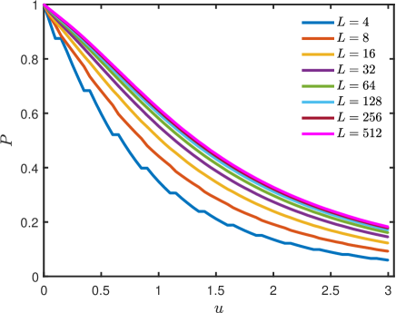
Figure 4: Largest cluster strength $P$ dependence on RW length parameter $u$ for $L=4,8,\dots,512$ (bottom left to top right). Each point is an average of $5\cdot 10^{5}$ configurations and the points are separated by $\Delta u=0.05$.

We denote the probability that a given site belongs to the largest cluster in the system as the largest cluster strength $P$. This is an ensemble average of the number of sites in the largest cluster divided by $L^{2}$. In Bernoulli percolation Stauffer and Aharony (1991) in the $L\to\infty$ limit, below the percolation threshold $P\to 0$ since the largest cluster is finite, while above the threshold $P$ is finite and represents the volume fraction of the infinite cluster. (Therefore, $P$ is used as an order parameter in many percolation problems.) Moreover, in Bernoulli percolation the concepts of infinite cluster and spanning cluster coincide. This is not the case in our problem. Due to the absence of a percolation threshold, the strength of the largest cluster $P$ includes both spanning and nonspanning clusters. In fact there is no significant difference in the volumes of both types of largest clusters and the volumes of all of them are proportional to $L^{2}$ leading to a finite $P$. Clearly, $P\leq p$ but this is a weak bound since $p\to 1$ as $L$ increases. Figure 4 depicts the largest cluster strength as a function of $u$ for lattice sizes $L$ ranging from 4 to 512. (As in Fig. 3, the steps for $L=4$ are due to truncation of $uL^{2}$ to an integer value.) As expected, $P(L,0)=1$ since the entire lattice is a single (largest) cluster, and the function monotonically decreases with increasing $u$. We observe that the graphs in Fig. 4 converge as $L\to\infty$ to a smooth function $P(\infty,u)$, confirming that the volume of the largest cluster scales as $L^{2}$. This observation will play an important role in Sec. IV. The convergence of the curves to $P(\infty,u)$ is significantly slower than the convergence of $\Pi$ in Fig. 3, since it is influenced by the slow approach of $p$ to unity, as indicated by Eq. (3): The analysis of the data for a single value of $u=u^{*}$ for larger $L$s shows some weak (but linear) dependence of $P$ on $1/\ln L$ indicating that the asymptotic value is by some 3% higher than the value for $L=512$.

The statistics of smaller clusters are of great interest in percolation problems. We define all the clusters except the largest cluster as finite clusters. We denote by $N_{s}$ the number of finite clusters with volume (number of sites) $s$ in a particular configuration on a lattice, and define the mean normalized cluster number $n_{s}=\langle N_{s}\rangle/L^{2}$, where $\langle\rangle$ denotes average over realizations. The exclusion of the largest cluster from the statistics resembles a similar definition in Bernoulli percolation Stauffer and Aharony (1991). However, in the latter case, it serves as a technical tool to exclude the infinite cluster above the percolation threshold, and plays a negligible role below the threshold where the size of the clusters is limited by $\xi$ and for large $L$ there are many clusters of similar sizes. Thus, in the “thermodynamic limit” of Bernoulli percolation the quantity $n_{s}$ is simply a function describing the prevalence of finite clusters. In 2DVSP the largest cluster always has its number of sites proportional to $L^{2}$ as do large “finite” clusters. From the definition of $n_{s}$ we see that $sN_{s}=sn_{s}L^{2}$ is the total number of sites belonging to finite clusters of size $s$ and therefore obtain the identity

$$\sum_{s}sn_{s}=p-P.$$ (4)

Unlike the case of Bernoulli percolation, the function $n_{s}$ may depend on $L$ and it is not evident that a limiting function exists for large $L$. We thoroughly discuss this function in Sec. V.

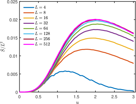
Figure 5: Ratio of the mean finite cluster size $\tilde{S}$ and system size $L^{2}$ as a function of RW length parameter $u$, for $L=4,8,\dots,512$ (bottom to top). Each point is an average of $5\cdot 10^{5}$ configurations and the points are separated by $\Delta u=0.05$.

The function $n_{s}$ can be used to determine the mean size of finite clusters: the total number of lattice sites which belong to an $s$ cluster is $sN_{s}$, and the total number of vacant sites is $pL^{2}$, then the probability that a randomly selected vacant site belongs to a finite $s$ cluster is $sn_{s}/p$, and the mean finite cluster size $\tilde{S}$ is

$$\tilde{S}=\frac{\sum_{s}s^{2}n_{s}}{p}\ .$$ (5)

This definition of the mean cluster size differs from a similar definition in Ref. Stauffer and Aharony (1991) only by the exclusion of the largest cluster in each configuration in the definition of $n_{s}$.

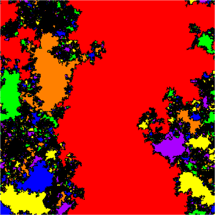
(a)

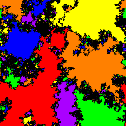
(b)

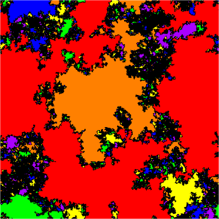
(c)

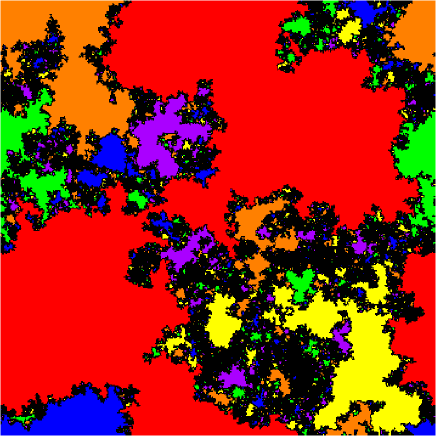
(d)

Figure 6: Examples of configurations on a $512\times 512$ lattice with $u=1.3$. The sites visited by the random walk are colored black. The clusters of vacant sites are colored according to their volume: the largest cluster is colored red, and the rest of the clusters are colored from the second largest to the smallest according to a periodic color scheme of orange, yellow, green, blue, violet. (In grayscale format these appears as different shades of gray with red $\rightarrow$ intermediate gray, blue $\rightarrow$ very dark gray, violet $\rightarrow$ dark gray, orange $\rightarrow$ light gray, green $\rightarrow$ very light gray, yellow $\rightarrow$ white.) The clusters can connect sites through the left and right edges of the lattice but not through the top and bottom edges. The examples include (a) a single large percolating cluster, (b) a nonpercolating system with three large clusters, (c) a very large and convoluted percolating cluster, and (d) a large percolating cluster with a narrow bottleneck.

In regular percolation the mean size of finite clusters is controlled by the correlation length $\xi$, which increases as the percolation threshold is approached. However, for $L\gg\xi$ the distribution $n_{s}$ becomes independent of $L$. In our problem $\tilde{S}\sim L^{2}$, and therefore Fig. 5 depicts the ratio $\tilde{S}/L^{2}$ as a function of $u$ for lattice sizes $L$ ranging from $4$ to $512$. (As in the previous figures, the steps in the $L=4$ graph are due to truncation to integer $N$.) The curves vanish for $u=0$ since the entire system is a single largest cluster which is excluded in the calculation of $n_{s}$. The values of $\tilde{S}$ increase with increasing $u$ until $u\sim 2$ and then decrease when the RW occupies most of the space for larger $u$. The ratio $\tilde{S}/L^{2}$ seems to converge as $L\to\infty$, confirming that even the mean finite cluster size scales as $L^{2}$. However, even here the numerical test of convergence of the function for a single $u=u^{*}$ indicates that there is a residual dependence on $1/\ln L$ leading to a slightly larger (up to 3%) limiting value of $\tilde{S}/L^{2}$. From our data it is not possible to determine whether the maximum of the curves keeps shifting with increasing $L$. Note that the mean size of the finite clusters at its maximum is only $\sim 0.02L^{2}$ which is rather small compared to $P$.

IV Geometry and fractality of the largest cluster

In this section we take a closer look at the geometry of the largest cluster. Figure 6 depicts four 2DVSP realizations for $L=512$ and $u=u^{*}=1.3$. This particular value $u=u^{*}$ was selected because it maximizes $\left|\frac{d\Pi}{du}\right|$, and we expect to see clusters that are close to the transition between spanning and nonspanning state, where diverse and ramified configurations can be observed. At $u=u^{*}$ close to half of configurations percolate, but the peak in $\left|\frac{d\Pi}{du}\right|$ is very broad and most of the configurations are not very close to the transition point.

A casual visual inspection of the configurations in Fig. 6 indicates that the largest clusters have rather “compact” two-dimensional interiors and very jagged boundaries. (Similar statements can be made about the clusters of intermediate sizes.) We also note that the linear dimensions of large clusters are of the order of $L$. Below we quantify these observations.

In most percolation problems the system is homogeneous beyond the correlation length $\xi$ Stauffer and Aharony (1991). However, close to the percolation transition the correlation length $\xi$, which is the typical linear size of finite clusters, is much larger than the lattice constant $a$. In the broad range of distances $a\ll r\ll\xi$, fractal behavior can be observed: e.g., the mass of a cluster within some distance $r$ from one of its sites increases as $r^{d_{f}}$, where $d_{f}$ is the fractal dimension of the cluster. Alternatively, the probability to find a site belonging to the cluster at the distance $r$ from another site of the same cluster decreases as $1/r^{d_{\rm co}}$, where the fractal codimension $d_{\rm co}=d-d_{f}$ Strelniker et al. (2009). (The relation between $d_{f}$ and $d_{\rm co}$ is obtained by integrating the density to find the mass within the radius $r$.) Thus, the fractal dimension can be measured either by examining total cluster mass within some distance $r$ or by examining two-point correlation functions. The presence of fractal behavior is not always easy to ascertain: E.g., for Bernoulli percolation in $d=2$ the fractal dimension ${d_{f}=\frac{91}{48}\approx 1.9}$ Kapitulnik et al. (1984); Stauffer and Aharony (1991) is not very different from the embedding dimension.

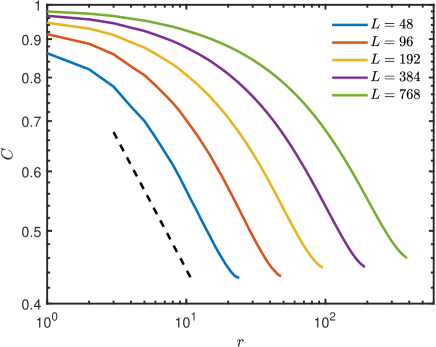
(a)

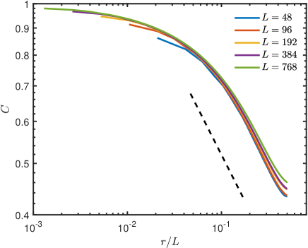
(b)

Figure 7: Logarithmic plot of the azimuthally averaged two-point correlation $C$ of the largest cluster (see text), averaged over $10^{3}$ samples, as a function of (a) distance between the points $r$, or (b) scaled distance $r/L$, for $L$ ranging from $48$ to $768$ [left to right in (a) and bottom to top in (b) with left-most points of the graphs from left to right]. The dashed line indicates slope $-0.35$.

In the presence of a percolation threshold, the “cluster mass versus radius” method for measuring the fractal dimension can be reduced to a measurement (at the threshold) of the mass $PL^{d}$ of the spanning cluster (part of the incipient infinite cluster) as a function of $L$ and equating it to $L^{d_{f}}$. Thus, the $L$ dependence of $P$ contains the information about $d_{f}$. In our problem the threshold is absent, while $P$ is independent of $L$, indicating the absence of fractal behavior, and confirming the impressions of Fig. 6. However, in 1985 Banavar et al. Banavar et al. (1985) examined two-point correlation functions of clusters of vacant sites left by a meandering RW at the percolation point in both $d=2$ and $3$ and reached the conclusion that these clusters exhibit fractal behavior. In $d=3$ their conclusion should not be surprising since the system has a percolation threshold and such behavior is expected. However, in $d=2$ they also found that $d_{f}=1.75$. Closely following their approach (see also Stauffer and Aharony (1991)), we define the two-point correlation function for the spanning cluster as

$$C(\vec{r})=\frac{1}{s}\sum_{\vec{r}\mkern 2.0mu\vphantom{r}^{\prime}}\rho\left(\vec{r}\mkern 2.0mu\vphantom{r}^{\prime}\right)\rho\left(\vec{r}+\vec{r}\mkern 2.0mu\vphantom{r}^{\prime}\right)\,,$$ (6)

where the density $\rho(\vec{r})$ equals $1$ for sites belonging to the spanning cluster (up to a lattice vector due to periodicity) and zero otherwise, and $\vec{r}\mkern 2.0mu\vphantom{r}^{\prime}$ is summed over all $s$ sites of the cluster.

Figure 7 depicts the azimuthal average of the correlation function $C$ for lattice sizes $L$ ranging from $48$ to $768$. All the graphs intersect at $r=0$ since by definition $C(0)=1$. The data for this figure were simulated using a different ensemble from the rest of our results: instead of a fixed $u$, the RW continues until the spanning cluster disconnects, and then we take the configuration of the lattice before the last step. This method creates an “almost disconnected” spanning cluster, and is similar to the methods used in Ref. Banavar et al. (1985). (We note that, while the length of the RWs in this ensemble is not fixed, the typical value of $u$ is $u\sim u^{*}$, consistently with Sec. III.) In Fig. 7(a) we see that for smaller fixed $r$, the correlation $C$ approaches a constant value independent of $r$ as $L$ increases. For larger $r$, the correlation function $C$ decays exhibiting finite size effects. E.g., the value of $r$ at which $C$ drops to, say, $0.6$, doubles every time $L$ is doubled. This is confirmed by the overlapping graphs in Fig. 7(b), where $C$ is displayed as a function of the scaled variable $r/L$.

Since the absolute value of the slope of each graph in Fig. 7 first increases for small $r$ and then decreases when $r$ approaches $L$, there is an intermediate regime on the logarithmic scale (less than $1/3$ of a decade) where the slope is almost constant, leading to an apparent power-law corresponding to codimension $d_{\rm co}=0.35$ (indicated by the dashed line). This behavior, although with a codimension $d_{\rm co}=0.25$ instead, prompted the authors of Ref. Banavar et al. (1985) to suggest that the spanning cluster is a fractal with dimension ${d_{f}=1.75}$ Banavar et al. (1985). Their data corresponds to $L=96$, which is the second left-most graph in Fig. 7(a). However, in the fractal regime, we would expect the $C(r)$ graphs corresponding to ever increasing $L$s to be linear continuations (on the logarithmic scale) of each other with their cutoffs ever increasing with $L$. Instead we see in Fig. 7(a) graphs that keep shifting to the right, clearly exhibiting a finite size ($L$ dependent) effect. We examined this for both the fixed $u$ and the “almost disconnected cluster” ensembles, and found no appreciable difference between the overall behavior of the correlation function. (It should be noted that when Ref. Banavar et al. (1985) was written, the absence of a critical point of 2DVSP was not clearly recognized.) These observations convince us that in $d=2$ the spanning cluster is indeed compact and its linear size is proportional to $L$, while its mass is proportional to $L^{2}$, consistently with the visual inspection of Fig. 6.

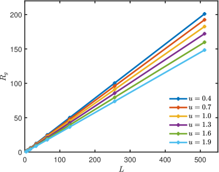
Figure 8: Radius of gyration $R_{g}$ of the largest cluster as a function of $L$ for $L=4,8,\dots,512$, and for $u=0.4,0.7,\dots,1.9$ (top left to bottom right). Each point is an average of $3\cdot 10^{5}$ configurations.

The linear size of a cluster can be quantified by its radius of gyration $R_{g}$, defined as Stauffer and Aharony (1991); Banavar et al. (1985)

$$R_{g}^{2}=\frac{1}{s}\sum_{i=1}^{s}(\vec{r}_{i}-\vec{r}_{\rm cm})^{2}\,,$$ (7)

where $s$ is the number of sites in the cluster, $\vec{r}_{i}$ are the cluster sites, and $\vec{r}_{\rm cm}$ is the position of the center of mass of the cluster. It should be noted that due to the periodic boundary conditions in the horizontal direction both the positions of steps $\{\vec{r}_{i}\}$ and the position of center of mass $\vec{r}_{\rm cm}$ are not always uniquely defined. The proper choices are made to minimize the resulting $R_{g}$. In regular percolation problems, the mean $R_{g}$ of the clusters, as well as $R_{g}$ of typical large clusters scale as the correlation length $\xi$.

We examined the relation between $R_{g}$ of various clusters and their mass for clusters in the entire range of sizes $s$. The particular values of the linear extent $R_{g}$ of various clusters with a given specific mass $s$ are broadly scattered, but the average values of $R_{g}^{2}(s)$ are proportional to $s$, leading to the conclusion that the clusters are not fractal, similarly to the largest cluster. Figure 8 depicts $R_{g}$ of the largest cluster as a function of $L$, for $L$ ranging from $4$ to $512$ and for $u=0.4,0.7,...,1.9$. We see that $R_{g}$ clearly displays the expected linear scaling with $L$, although the slope of linear curves in Fig. 8 slowly decreases with increasing $u$.

The jagged boundary of the clusters seen in Fig. 6 is formed by segments of a RW. We define the cluster hull perimeter $H$ as the total mass of cluster sites bordering the sites visited by the random walk. We considered the hull perimeter only for the largest cluster. For fixed $L$ we may expect the numerical value of the perimeter to decrease as $u\to 0$ since the spanning cluster will essentially have no boundaries, and on the other hand for $u\gg 1$ the perimeter will again be small due to a decrease in the typical size of the largest cluster. Somewhere at the intermediate values of $u$, possibly around $u^{*}$, we will see large hull perimeters. Unlike Bernoulli percolation, our clusters do not have internal boundaries due to holes inside a cluster, and therefore their entire perimeter belongs to the hull. For Bernoulli site percolation at $d=2$ and $p=p_{c}$, both the mass and the hull of the spanning cluster are fractal, and the hull scales as $H\sim L^{D_{H}}$ with fractal dimension $D_{H}=1.74$ Grossman and Aharony (1986); Voss (1984).

Figure 9 depicts the hull perimeter $H$ of the largest cluster of our problem as a function of $L$, for $L$ ranging from $4$ to $512$ and for $u=0.4,0.7,...,1.9$ on a logarithmic scale. For a fixed large $L$ the hull perimeter $H$ slightly depends on $u$ reaching a maximum close to $u=1.0$ (see inset in the figure). With increasing $L$ all of the graphs approach straight lines with slopes corresponding to a power $D_{H}=1.33\pm 0.01$, where the size of the error provides a subjective estimate of uncertainty in extrapolation as well as slight differences between different values of $u$. The dashed line in Fig. 9 has a slope of 4/3 and provides a guide to the eye. (The statistical errors are negligible.) The measured exponent of 4/3 coincides with the well-known theoretical result proven by Lawler et al. Lawler et al. (2001) (and conjectured by Mandelbrot Mandelbrot (1982)) that the fractal dimension of the frontier of a Brownian motion in $d=2$ is $4/3$.

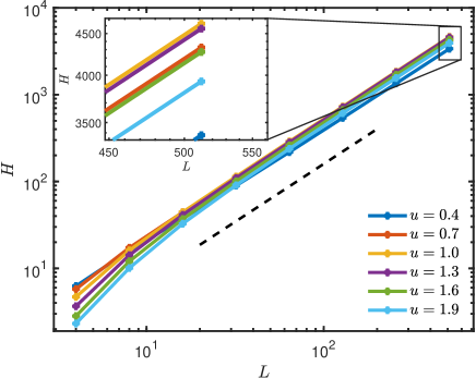
Figure 9: Logarithmic plot of the hull perimeter $H$ of the largest cluster as a function of $L$ for $L=4,8,\dots,512$, and for $u=0.4,0.7,\dots,1.9$ with left-most points of the graphs from top to bottom. Some of the lines intersect, and the right-most points (shown enlarged in the inset) are ordered from top to bottom in order $u=1.0,1.3,0.7,1.6,1.9,0.4$, i.e., for larger $L$s the hull perimeter slightly increases as $u$ increases from 0.4 to 1.0 and then decreases. Each point is an average of $3\cdot 10^{5}$ configurations. The dashed line indicates slope $4/3$.

V Cluster Statistics

The mean number of clusters of size $s$ per lattice site $n_{s}$ as defined in Sec. III is one of the most revealing features of a percolating system. Despite the differences between 2DVSP and the usual Bernoulli percolation we will attempt to follow a similar logic while pointing out important differences between the systems. If a system lacks a length or mass scale, then we expect the functions characterizing the system to be power-laws. In particular, one might expect $n_{s}=As^{-\tau}$, where $\tau$ is called a Fisher exponent Stauffer and Aharony (1991), while $A$ is a constant, possibly dependent on some microscopic properties and details. In Bernoulli percolation such dependence is valid on scales $r$ much larger than the lattice constant $a$ but smaller than the correlation length $\xi$, i.e., for cluster masses satisfying $1\ll s\ll s_{c}$, where $s_{c}$ is a typical mass of a cluster of linear size $\xi$. (Typically, there is a power-law dependence between $s_{c}$ and $\xi$.) At length scales $r\sim\xi$ the power-law is corrected by some cutoff function $F_{c}$, which is $\approx 1$ for $s\ll s_{c}$ and drops to zero as $s_{c}$ is exceeded. The overall shape of the dependence is

$$n_{s}=As^{-\tau}F_{c}\,.$$ (8)

It is frequently assumed in Bernoulli percolation that the cutoff function depends only on the ratio $s/s_{c}$, although away from the threshold a more complicated dependence on $p$ might appear Ding et al. (2014). At the percolation threshold ($\xi=\infty$) the cutoff is absent, and therefore Eq. (4) dictates that an infinite sum $\sum_{s}sn_{s}\approx\sum_{s}As^{1-\tau}$ converges, and therefore $\tau>2$. Indeed for two-dimensional Bernoulli percolation $\tau=197/81\approx 2.05$ Stauffer and Aharony (1991).

In the 2DVSP problem the function $n_{s}$ plays a somewhat different role. In percolation problems with a threshold, there is some correlation length $\xi$ and therefore a very large system of linear size $L$ can be treated as a collection of $(L/\xi)^{d}$ independent systems. Consequently, even a single very large realization of the system assures that most cluster sizes $s$ will be present and $n_{s}$ can be naturally treated as a continuous function representing the frequency of clusters of size $s$. In the 2DVSP, there is no correlation length and $L$ is the only large length scale. In a single sample there are only a few large clusters of size $s\sim L^{2}$ and, consequently, if we avoid averaging over samples for most large $s$, we will have vanishing $n_{s}$ and only a few particular values of $s$ will produce $n_{s}=1/L^{2}$. An increase of $L$ will not improve that situation. Only averaging over the ensemble will produce a continuous function $n_{s}$ of $s$. Nevertheless, we expect to have a large range of scale-free behavior, and, as in the case of regular percolation, we hope that the ensemble averaged $n_{s}$ has a shape given by Eq. (8).

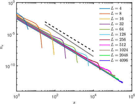
Figure 10: Logarithmic plot of $n_{s}$, averaged over $7\cdot 10^{5}$ samples, as a function of the cluster mass $s$, for $u=1.3$ and for $L=4,8,\dots,4096$ (left to right). [Curves for $L\geq 1024$ are truncated for large $s$ (see text).] The dashed and dotted lines indicate slopes $-1.85$ and 2, respectively.

Figure 10 depicts a logarithmic plot of the cluster number per site $n_{s}$ for $L$ ranging from $4$ to $4096$ and $u=1.3$. All the graphs consist of a relatively straight region for $s\ll L^{2}$ and a cutoff around $0.3L^{2}$. Close to the cutoff, the curves exhibit somewhat unusual behavior described in the next paragraph. We excluded the area close to the cutoff from our analysis of scaling behavior. While we used rather large statistical samples, the frequencies of finding a cluster of some particular (large) $s$ for large $L$s become very low and the resulting curves are very “noisy.” The curves presented in Fig. 10 are “smoothed” by averaging the results for a particular $s$ over a range $\sim\sqrt{s}$. This procedure has almost no effect for moderate $L$s, but distorts the “tails” of the curves on large lattices: for $L\geq 512$, when $n_{s}$ drops below a certain (small) value, where in the entire ensemble of $7\cdot 10^{5}$ samples there is about one cluster of each size $s$, the averaging procedure distorts the curve, because it is just an averaging of zeros and ones. We therefore truncate the curves when this value is reached. For $L=512$ the truncation appears when the cutoff is reached, while for larger $L$s the graphs are truncated even before reaching the cutoff.

All the curves for $L<512$ in Fig. 10 exhibit a sharp cutoff and the position of that cutoff increases by a factor of 4 every time $L$ doubles. Such $L$ dependence is consistent with the results that we had in Sec. III. Therefore, the cutoff function depends of $s/s_{c}$, with $s_{c}\sim L^{2}$ and with some dependence on $u$. Near the cutoff position the function $F_{c}$ has some structure: In Fig. 10 instead of being just a simple monotonic drop from 1 to 0, it actually increases above 1 before the drop thus moderating the decay of $n_{s}$ close to $s_{c}$. The behavior close to the cutoff depends on $u$: For smaller $u$s the “bump” in $F_{c}$ becomes even more pronounced. Such nontrivial shape of $F_{c}$ apparently reflects the fact that the large-$s$ part of $n_{s}$ attempts to depict few very large clusters by using a smooth function of $s$.

Before the cutoff, the curves in Fig. 10 are fairly straight and approximately follow a slope the absolute value of which very slowly increases and reaches the value of $\tau\approx 1.83$ (or slightly larger) for the largest $L$s. The dashed line in Fig. 10 indicates a slope of -1.85. Such behavior is a significant deviation from the expectation that $\tau$ should exceed 2. If this represents an asymptotic trend, then the requirement for $\sum_{s}sn_{s}$ to be finite for ever increasing $L$, i.e., with the power-law cutoff increasing as $L^{2}$, would require the prefactor of the power-law in Eq. (8) to decrease $A\sim L^{2(\tau-2)}$. While the vertical position of the curves in Fig. 10 slightly decreases with increasing $L$ it is extremely weak, possibly dependent on $1/\ln L$. Strong $L$ dependence of $A$ would also cast doubt on our assumption of scale-independence of the results on the intermediate scales. The results described in this paragraph, namely $\tau<2$ and $A$ almost independent of $L$, are not mutually consistent.

Special properties of Gaussian RWs in $d=2$ can be used to advance a theoretical heuristic argument that the theoretical value of $\tau$ should be $\tau_{\rm th}=2$. Long RWs on a lattice can be treated as Gaussian RWs in a continuum. As has been mentioned in Sec. II, a Gaussian RW can be coarse-grained or fine-grained exactly: The increase of lattice size from $L$ to $\lambda L$ and number of steps $N$ from $uL^{2}$ to $u\lambda^{2}L^{2}$ is equivalent to keeping the system size unchanged, while increasing $N$ by a factor $\lambda^{2}$ and decreasing the step size $\ell$ by factor $\lambda$. Positions of every $\lambda^{2}$rd step of this new fine-grained configuration will be distributed exactly as the positions of the original Gaussian RW before it was fine-grained. Thus, the process of fine-graining replaces each step of the RW by $\lambda^{2}$ smaller steps but does not change the paths of RWs on larger scales. We saw in Sec. IV that the clusters have compact interiors, and therefore their volume will not change, except for being measured in smaller units, i.e., a cluster of $s$ sites will become a cluster of $\lambda^{2}s$ sites, of the same shape, although with more jagged boundaries. This argument, as mentioned in in Sec. II assumes that the slight changes in the fine-grained boundaries created by the RW do not break up fragile clusters that have bottlenecks or join clusters which were “almost connected” in the original geometry, or at least such changes are very rare and do not modify the distributions. The change of scale will certainly have effect on creation or elimination of the smallest clusters. Thus by assuming that nothing changed in the overall geometry we find that the number of clusters in a certain range $N_{s}(L)\Delta s$ remains unchanged in the new units, i.e., it is equal to $N_{\lambda^{2}s}(\lambda L)\Delta(\lambda^{2}s)$. This equality is valid only for large enough $s$, far from the smallest $s$ where the cluster number is dependent on the resolution and graining. By dividing both terms by $L^{2}$ and eliminating $\Delta s$ we find that

$$n_{s}(L)=\lambda^{4}n_{\lambda^{2}s}(\lambda L).$$ (9)

The argument presented above assumed $\lambda>1$ and resulted in fine-graining of the system. We could use $\lambda<1$ and coarse grain the system. The resulting relation is valid for arbitrary $\lambda$, and, in particular, by taking $\lambda=1/L$ we observe that $L^{4}n_{s}(L)$ becomes a function of only of $s/L^{2}$. Figure 11 depicts the scaled number of clusters as a function of the scaled cluster mass, and the graphs for various $L$s almost (but not completely) collapse. Furthermore, the scaled cutoffs are very similar and appear at about $s_{c}/L^{2}\approx 0.3$, yet again confirming relation $s_{c}\sim L^{2}$.

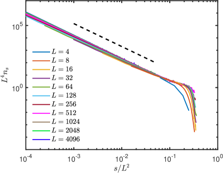
Figure 11: Logarithmic plot of $L^{4}n_{s}$, averaged over $7\cdot 10^{5}$ samples, as a function of the scaled cluster mass $s/L^{2}$, for $u=1.3$ and for $L=4,8,\dots,4096$ (bottom to top, which is left to right at the right ends of the graphs). [Curves for $L\geq 1024$ are truncated for large $s$ (see text).] This is a scaled version of the data in Fig. 10. The dashed line indicates slope $-1.85$.

The left hand side of Eq. (9) is independent of $\lambda$, and the equation must be valid for an arbitrary $\lambda$ in the power-law regime that is only possible, when $n_{s}=As^{-2}$ leading to the “theoretical” value of the Fisher exponent $\tau_{\rm th}=2$. A slope of -2 is indicated by the dotted line in Fig. 10, and seems to be slightly larger than the approximate slope of -1.83 seen in the graph. Later we will explore the possibility that our results did not yet converge to their asymptotic values. If the Fisher exponent is 2, then the coefficient $A$ cannot be constant: to maintain a finite $\sum_{s}sn_{s}$, it must decrease as $1/\ln L$. Indeed, $A$ slowly decreases with increasing $L$. Our heuristic argument is not accurate enough to determine the logarithmic terms either in the prefactor, or even in the $s$ dependence of $n_{s}$.

In Sec. III we discussed the possibility of extremely slow convergence of the numerical results when the $L$ dependence may be as slow as $1/\ln L$. We attempted to study the apparent discrepancy between the heuristic result $\tau_{\rm th}=2$ and the measured $\tau\approx 1.83$. We measured the weak dependence on $L$ of the effective exponent $\tau$. The exponent has been extracted from a linear fit on a logarithmic scale in the range $1\leq s\leq 0.01L^{2}$, which avoids the very peculiar behavior of the curves near the cutoff. The data points for $\tau$ in Fig. 12 are arithmetic means of the slopes in the two halves of the range, $1<s<0.1L$ and $0.1L<s<0.01L^{2}$. Figure 12 depicts $\tau$ as a function of $1/\ln{L}$ for $L=64,128,256,512$ and for ${u=0.7,1.0,\dots,2.8}$. For $u=1.3$ the simulations have been extended to $L=1024,2048,4096$. Slightly nonlinear behavior (on the logarithmic scale) of the graphs in Fig. 10 introduces possible systematic errors as large as $0.05$. Such errors, combined with extremely slow $L$ dependence prevent a reliable extrapolation to $L\to\infty$. Nevertheless, Fig. 12 demonstrates the plausibility of the asymptotic value $\tau_{\rm th}=2$ that is indicated by an arrow.

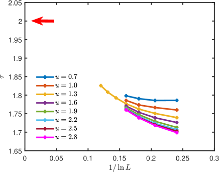
Figure 12: Plot of the effective exponents $\tau$ defined in Eq. (8), as a function of $1/\ln{L}$, for $u=0.7,1.0,...,2.8$ (top to bottom) and $L=64,128,256,512$. For $u=1.3$ the range of $L$s was extended to $L=1024,2048,4096$. The exponents are extracted from linear fits (on logarithmic scale) in the range $1\leq s\leq 0.01L^{2}$ (see text). Estimated systematic errors in vertical positions of data points are as large as 0.05. The arrow near the vertical axis indicates the expected theoretical value $\tau_{\rm th}=2$, rather than a value extrapolated from data.

Usage of the continuous (ensemble averaged) function $n_{s}$ obscures the fact that there are only a few large clusters, and therefore in each sample there are no clusters for most large values of $s$. It is therefore beneficial to examine these statistics from a different point of view. We denote by $P_{k}$ the mass (volume) of the $k$th largest cluster, divided by the lattice volume $L^{2}$, and averaged over realizations. In particular, the largest cluster strength $P$ equals $P_{1}$, and the identity ${\sum_{k}P_{k}=p}$ is trivial. By construction $P_{k}$ is monotonous and should exhibit a more “continuous” behavior than $n_{s}$ because for large clusters (small $k$), $P_{k}$ should converge in the $L\to\infty$ limit just as $P$ does, and for smaller clusters the differences between cluster sizes are small and there are many of them.

Figure 13 depicts $P_{k}$ as a function of the cluster mass index $k$, for $L$ ranging from $4$ to $4096$ and $u=1.3$. The graphs are obtained from the average of $P_{k}$ over many configurations, in the same manner as the graphs of $n_{s}$ in Fig. 10. For $k>10$ the graphs appear to roughly converge to a straight line representing a power law $Bk^{-q}$, up to a sharp cutoff $k_{c}$ which increases with increasing $L$. The effective exponent $q$ slightly decreases with increasing $L$ and reaches $q=1.20$ for the largest sample. (The estimated systematic errors of the effective exponents are smaller than 0.05.) The prefactor $B$ is almost independent of $L$. We note that most of the mass of the vacant clusters is contained in three or four largest clusters, while the remainder contains a small fraction of vacant sites. Since large $k$ corresponds to small clusters, the value of $k_{c}$ is not evident. Clearly, the total number of clusters is significantly smaller than the number of sites, and therefore $k_{c}\ll L^{2}$. Even a tighter bound can be obtained by demanding the cutoff appears when the cluster sizes reach a single site, i.e., $k_{c}\approx L^{2/q}B^{1/q}$. The changing shape of the cutoff does not permit exact evaluation of its power dependence on $L$ but it seems to increase slightly slower than $L^{2}$.

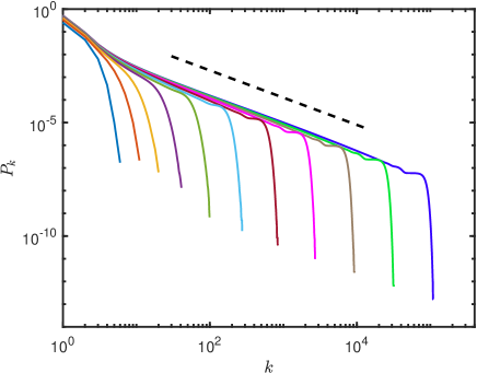
Figure 13: Logarithmic plot of $P_{k}$, averaged over $7\cdot 10^{5}$ samples, as a function of the cluster mass index $k$, for $u=1.3$ and for $L=4,8,\dots,4096$ (left to right). The dashed line indicates slope $-1.20$.

Both $P_{k}$ and $n_{s}$ describe the same cluster statistics from slightly different points of view. Assuming that they both are power-laws, it should be possible to relate them. The cluster size $s$ for a specific fixed index $k$ fluctuates, but it is possible to treat the mean of $s$ as a function of $k$. Similarly, for a specific $s$ we can define the mean value of $k$. Both of these $s$–$k$ relations are expected to be the same power-laws. As long as the fluctuations of $s$ for fixed $k$, or, alternatively, the fluctuations of $k$ for fixed $s$ are small, we can proceed with our derivation by assuming an approximate deterministic relation $s(k)$. (For power-law distributions such a relation can be used even when the fluctuations are large: one gets correct relations between the exponents.) We will extract this relation from the mass of the $k$th cluster $L^{2}P_{k}=L^{2}Bk^{-q}=s$. If there are $N_{s}$ clusters of size $s$, the change of an $s$ cluster’s mass by a unit advances its cluster index $k$ by $N_{s}$. Therefore, we expect ${\frac{dk}{ds}=-N_{s}}$, or

$$\frac{dk}{d\left(L^{2}Bk^{-q}\right)}=-L^{2}As^{-\tau}=-L^{2}A(L^{2}Bk^{-q})^{-\tau}\ ,$$ (10)

which relates the exponents $q$ and $\tau$ by

$$q=\frac{1}{\tau-1}\ .$$ (11)

The slope of the graphs in Fig. 13 indicates that $q\approx 1.20$, and this corresponds due to Eq. (11) to $\tau\approx 1.83$. The latter value is the same as the (approximate) measured value of $\tau$ in the graphs of Fig. 10. It is interesting to note that that our heuristic estimate $\tau_{\rm th}=2$ corresponds to the exponent $q=q_{\rm th}=1$. By examining the dependence of the effective exponent $q$ on $1/\ln L$ we note that 1 is the likely asymptotic value of $q$ for $L\to\infty$, although large error bars prevent exact extrapolation. Further examination of the coefficients in Eq. (10) shows that the product of the prefactors $AB^{1-\tau}\sim L^{2(\tau-2)}$. Since neither $A$ nor $B$ show significant $L$ dependence, the anticipated asymptotic value $\tau=\tau_{\rm th}=2$ seems to be consistent with our results.

VI Conclusions and Discussion

The study of RWs in $d=2$ is a very old and well explored subject. We concentrated on percolation aspects of sites not visited by the random walk on a periodic lattice both because this is the lower critical dimension of a slightly more conventional percolation problems of vacant sites in $d\geq 3$, and because this problem exhibits features that are absent in “typical” lower critical dimension problems. As far as it was possible, we used the tools of percolation theory to analyze the problem, although certain features were very different from regular percolation, and even different from the behavior of Bernoulli percolation at its lower critical dimension.

Our paper was motivated by $d=2$ being the lower critical dimension of a practically more important problem of gel degradation problem in $d=3$. However, cross-linked membranes are ubiquitous in biology and medicine, and their degradation, artificial or natural, plays an important role warranting the consideration of degradation by an enzyme. Two-dimensional processes with RW-controlled connectivity are also related to certain models of photosynthetic bacteria colonies or photosynthetic membranes in which the energy of light is transmitted to neighboring areas via excitons thus creating correlations (see Ref. de Rivoyre et al. (2010) and references therein). However, such correlations are short-lived and the problem crosses over to Bernoulli percolation behavior d’Auriac and Iglói (2021).

We have demonstrated that contrary to older results, the cluster interiors are not fractal, although their boundaries are. The only macroscopic scale of the 2DVSP problem is the lattice size $L$ and at shorter distances the behavior is scale-free and can be described using power-laws. The 2DVSP problem converges very slowly to the “large $L$ limit.” Our results indicate that the approach to asymptotic behavior is as slow as the decay to zero of $1/\ln L$. Consequently, all measurements even at large $L$ correspond to intermediate effective behavior. We suggested a heuristic argument setting the values of the exponents $\tau$ and $q$ describing the cluster size distribution. Measured values of the exponents are distinct but seem to move towards the theoretical values with increasing $L$.

For $u\ll 1$ the problem of cluster size distribution can be described on an infinite lattice without the need to introduce periodic boundary conditions. For $u\gg 1$ the spanning clusters are virtually nonexistent and one needs to understand clusters created by ${\cal N}_{\rm cr}\gg 1$ almost independent pieces of the RW. Most of our measurements were performed for $u=O(1)$, where the situation is most diverse, and might be different from the behavior at very small or very large $u$s. Our paper does not resolve this problem. Moreover, the approach to the limit of $p\to 1$ is much slower for larger $u$ values, and therefore various parts of the curves, such as shown in Figs. 3 to 5, converge at different rates to their asymptotic values. Therefore the shape of the curves may keep changing with increasing $L$.

The graphs in Fig. 13 have a rather distinct behavior for $k\lesssim 4$ as opposed to larger $k$s. Such a separation into “large” clusters (small $k$), and ”small” clusters (larger $k$) provides possible clues into the $u$ dependence of the features. By examining similar graphs for different values of $u$ we observed that increasing $u$ decreases the sizes of the “large” clusters, but increases the sizes of the clusters with larger $k$ towards the larger cluster sizes. The $u$ dependence of all the properties requires a more systematic study.

Our theoretical arguments did not go beyond an approximate “heuristic” approach. However, a RW is a rather well understood object, and it is conceivable that more accurate predictions can be made analytically.