An Assessment of Different Electronic Structure Approaches for Modeling Time-Resolved X-ray Absorption Spectroscopy

Abstract

We assess the performance of different protocols for simulating excited-state X-ray absorption spectra. We consider three different protocols based on equation-of-motion coupled-cluster singles and doubles, two of them combined with the maximum overlap method. The three protocols differ in the choice of a reference configuration used to compute target states. Maximum-overlap-method time-dependent density functional theory is also considered. The performance of the different approaches is illustrated using uracil, thymine, and acetylacetone as benchmark systems. The results provide a guidance for selecting an electronic structure method for modeling time-resolved X-ray absorption spectroscopy.

I Introduction

Since the pioneering study by Zewail’s group in the mid-eighties, Scherer et al. (1985) ultrafast dynamics has been an active area of experimental research. Advances in light sources provide new means for probing dynamics by utilizing core-level transitions. X-ray free electron lasers (XFELs) and instruments based on high-harmonic generation (HHG) enable spectroscopic measurements on the femtosecond Young et al. (2018); Chergui and Collet (2017); Ueda (2018) and attosecondCalegari et al. (2016); Ramasesha, Leone, and Neumark (2016); Ischenko, Weber, and Miller (2017); Villeneuve (2018) timescales. Methods for investigating femtosecond dynamics can be classified into two categories: $(i)$ methods that track the electronic structure as parametrically dependent on the nuclear dynamics, such as time-resolved photoelectron spectroscopy (TR-PES), Schuurman and Stolow (2018); Adachi and Suzuki (2018); Suzuki (2019); Liu et al. (2020) and $(ii)$ methods that directly visualize the nuclear dynamics, such as ultrafast X-ray scattering Glownia et al. (2016); Stankus et al. (2019); Ruddock et al. (2019); Stankus et al. (2020) and ultrafast electron diffraction. Yang et al. (2016); Liu et al. (2020) Time-resolved X-ray absorption spectroscopy (TR-XAS) belongs to the former category. Similarly to X-ray photoelectron spectroscopy (XPS), XAS is also element and chemical-state specific Stöhr (1992) but is able to resolve the underlying electronic states better than TR-XPS. On the other hand, TR-XPS allows photoelectron detection from all the involved electronic states with higher yield. XAS has been used to probe the local structure of bulk-solvated systems, such as in most chemical reaction systems in the lab and in cytoplasm. TR-XAS has been employed to track photo-induced dynamics in organic molecules Pertot et al. (2017); Attar et al. (2017); Wolf et al. (2017); Bhattacherjee et al. (2017) and transition metal complexes. Chen, Zhang, and Shelby (2014); Chergui (2016); Chergui and Collet (2017); Wernet (2019) With the aid of simulations, Katayama et al. (2019) nuclear dynamics can be extracted from experimental TR-XAS spectra.

Similar to other time-resolved experimental methods from category $(i)$, interpretation of TR-XAS relies on computational methods for simulating electronic structure and nuclear wave-packet dynamics. In this context, electronic structure calculations should be able to provide: (1) XAS of the ground states; (2) a description of the valence-excited states involved in the dynamics; (3) XAS of the valence-excited states.

Quantum chemistry has made a major progress in simulations of XAS spectra of ground states. Norman and Dreuw (2018); Bokarev and Kühn (2020) Among the currently available methods, the transition-potential density functional theory (TP-DFT) with the half core-hole approximation Triguero, Pettersson, and Ågren (1998); Leetmaa et al. (2010) is widely used to interpret the XAS spectra of ground states. Vall-llosera et al. (2008); Perera and Urquhart (2017) Ehlert et al. extended the TP-DFT method to core excitations from valence-excited states, Ehlert, Gühr, and Saalfrank (2018) and implemented it in PSIXAS, Ehlert and Klamroth (2020) a plugin to the Psi4 code. TP-DFT is capable of simulating (TR-)XAS spectra of large molecules with reasonable accuracy, as long as the core-excited states can be described by a single electronic configuration. Other extensions of Kohn-Sham DFT, suitable for calculating the XAS spectra of molecules in their ground states, also exist. Michelitsch and Reuter (2019) Linear response (LR) time-dependent (TD) DFT, a widely used method for excited states, Dreuw and Head-Gordon (2005); Luzanov and Zhikol (2012); Laurent and Jacquemin (2013); Ferré, Filatov, and Huix-Rotllant (2016) has been extended to the calculation of core-excited states Stener, Fronzoni, and de Simone (2003); Besley and Asmuruf (2010) by means of the core-valence separation (CVS) scheme, Cederbaum, Domcke, and Schirmer (1980) a specific type of truncated single excitation space (TRNSS) approach. Besley (2004) In the CVS approach, configurations that do not involve core orbitals are excluded from the excitation space; this is justified because the respective matrix elements are small, owing to the localized nature of the core orbitals and the large energetic gap between the core and the valence orbitals.

Core-excitation energies calculated using TDDFT show errors up to $\approx$20 eV when standard exchange-correlation (xc) functionals such as B3LYP Becke (1993) are used. The errors can be reduced by using specially designed xc-functionals, such as those reviewed in Sec. 3.4.4. of Ref. 27. Hait and Head-Gordon recently developed a square gradient minimum (SGM) algorithm for excited-state orbital optimization to obtain spin-pure restricted open-shell Kohn-Sham (ROKS) energies of core-excited states; they reported sub-eV errors in XAS transition energies. Hait and Head-Gordon (2020a)

The maximum overlap method (MOM) Gilbert, Besley, and Gill (2008) provides access to excited-state self-consistent field (SCF) solutions and, therefore, could be used to compute core-level states. More importantly, MOM can be also combined with TDDFT to compute core excitations from a valence-excited state. Attar et al. (2017); Bhattacherjee et al. (2017); Northey et al. (2020) MOM-TDDFT is an attractive method for simulating TR-XAS spectra, because it is computationally cheap and may provide excitation energies consistent with the TDDFT potential energy surfaces, which are often used in the nuclear dynamics simulations. However, in MOM calculations the initial valence-excited states are independently optimized and thus not orthogonal to each other. This non-orthogonality may lead to flipping of the energetic order of the states. Moreover, open-shell Slater determinants provide a spin-incomplete description of excited states (the initial state in an excited-state XAS calculation), which results in severe spin contamination of all states and may affect the quality of the computed spectra. Hait and Head-Gordon have presented SGM as an alternative general excited-state orbital-optimization method Hait and Head-Gordon (2020b) and applied it to compute XAS spectra of radicals. Hait et al. (2020)

Applications of methods containing some empirical component, such as TDDFT, require benchmarking against the spectra computed with a reliable wave-function method, whose accuracy can be systematically assessed. Among various post-HF methods, coupled-cluster (CC) theory yields a hierarchy of size-consistent ansätze for the ground state, with the CC singles and doubles (CCSD) method being the most practical. Bartlett and Musiał (2007) CC theory has been extended to excited states via the linear response Koch and Jørgensen (1990); Christiansen, Jørgensen, and Hättig (1998); Sneskov and Christiansen (2012) and the equation-of-motion for excited states (EOM-EE) Stanton and Bartlett (1993); Krylov (2008); Bartlett (2012); Coriani et al. (2016) formalisms. Both approaches have been adapted to treat core-excited states by using the CVS scheme, Coriani and Koch (2015) including calculations of transition dipole moments and other properties. Vidal et al. (2019); Tsuru et al. (2019); Faber et al. (2019); Nanda et al. (2020); Faber and Coriani (2020); Vidal, Krylov, and Coriani (2020a); Vidal et al. (2020a) The benchmarks illustrate that CVS-enabled EOM-CC methods describe well the relaxation effects caused by the core hole as well as differential correlation effects. Given their robustness and reliability, CC-based methods provide high-quality XAS spectra, which can be used to benchmark other methods. Beside several CCSD investigations, Coriani et al. (2012); Coriani and Koch (2015); Frati et al. (2019); Carbone et al. (2019); Wolf et al. (2017); Peng et al. (2015); Tsuru et al. (2019); Fransson et al. (2013); Vidal et al. (2019); Sarangi et al. (2020); Tenorio et al. (2019); Moitra et al. (2020); Vidal et al. (2020a, b) core excitation and ionization energies have also been reported at the CC2, Coriani et al. (2012); Carbone et al. (2019); Frati et al. (2019); Costantini et al. (2019); Moitra et al. (2020) CC3 Wolf et al. (2017); Myhre et al. (2018); Folkestad et al. (2020); Paul, Myhre, and Koch (2021), CCSDT,Carbone et al. (2019); Myhre et al. (2018); Matthews (2020) CCSDR(3), Coriani et al. (2012); Matthews (2020); Moitra et al. (2020) and EOM-CCSD*Matthews (2020) levels of theory. XAS spectra have also been simulated with a linear-response (LR-) density cumulant theory (DCT), Peng, Copan, and Sokolov (2019) which is closely related to the LR-CC methods.

The algebraic diagrammatic construction (ADC) approach Schirmer (1982); Dreuw and Wormit (2015) has also been used to model inner-shell spectroscopy. The second-order variant ADC(2) Barth and Schirmer (1985) yields valence-excitation energies with an accuracy and a computational cost [$O(N^{5})$] similar to CC2 (coupled-cluster singles and approximate doubles), Christiansen, Koch, and Jørgensen (1995) but within the Hermitian formalism. ADC(2) was extended to core excitations by the CVS scheme. Schirmer et al. (1993); Wenzel, Wormit, and Dreuw (2014) Because ADC(2) is inexpensive and is capable of accounting for dynamic correlation when calculating potential energy surfaces, Plasser et al. (2014a) it holds promise of delivering reasonably accurate time-resolved XAS spectra at a low cost at each step of the nuclear dynamic simulation. Neville et al. simulated TR-XAS spectra with ADC(2), Neville et al. (2016a, b, 2018) while using multi-reference first-order configuration interaction (MR-FOCI) in their nuclear dynamics simulations. Neville and Schuurman also reported an approach to simulate XAS spectra using electronic wave packet autocorrelation functions based on TD-ADC(2). Neville and Schuurman (2018) An ad hoc extension of ADC(2), ADC(2)-x, Trofimov and Schirmer (1995) is known to give ground-state XAS spectra with relatively high accuracy (better than ADC(2)) employing small basis sets such as 6-31+G, Plekan et al. (2008) but the improvement comes with a higher computational cost $[O(N^{6})]$. List et al. have recently used ADC(2)-x, along with RASPT2, to study competing relaxation pathways in malonaldehyde by TR-XAS simulations. List et al. (2020)

An important limitation of the single-reference methods (at least those only including singles and double excitations) is that they can reliably treat only singly excited states. While transitions to the singly occupied molecular orbitals (SOMO) result in target states that are formally singly excited from the ground-state reference state, other final states accessible by core excitation from a valence-excited state can be dominated by configurations of double or higher excitation character relative to the ground-state reference. Consequently, these states are not well described by conventional response methods such as TDDFT, LR/EOM-CCSD, or ADC(2) (see Fig. 2 in II.1). Tsuru et al. (2019); List et al. (2020) This is the main rational of using MOM within TDDFT.

To overcome this problem while retaining a low computational cost, Seidu et al. Seidu et al. (2019) suggested to combine DFT and multireference configuration interaction (MRCI) with the CVS scheme, which led to the CVS-DFT/MRCI method. The authors demonstrated that the semi-empirical Hamiltonian adjusted to describe the Coulomb and exchange interactions of the valence-excited states Lyskov, Kleinschmidt, and Marian (2016) works well for the core-excited states too.

In the context of excited-state nuclear dynamics simulations based on complete active-space SCF (CASSCF) or CAS second-order perturbation theory (CASPT2), popular choices for computing core excitations from a given valence-excited state are restricted active-space SCF (RASSCF) Olsen et al. (1988); Malmqvist, Rendell, and Roos (1990) or RAS second-order perturbation theory (RASPT2). Malmqvist et al. (2008) Delcey et al. have clearly summarized how to apply RASSCF for core excitations. Delcey et al. (2019) XAS spectra of valence-excited states computed by RASSCF/RASPT2 have been presented by various authors. Hua, Mukamel, and Luo (2019); Segatta et al. (2020); Northey et al. (2020) RASSCF/RASPT2 schemes are sufficiently flexible and even work in the vicinity of conical intersections; they also can tackle different types of excitations, including, for example, those with multiply excited character.Schweigert and Mukamel (2007) However, the accuracy of these methods depends strongly on an appropriate selection of the active space, which makes their application system-specific. In addition, RASSCF simulations might suffer from insufficient description of dynamic correlation whereas the applicability of RASPT2 may be limited by its computational cost.

Many of the methods mentioned above are available in standard quantum chemistry packages. Hence, the assessment of their performance would be valuable help for computational chemists who want to use these methods to analyze the experimental TR-XAS spectra. Since experimental TR-XAS spectra are still relatively scarce, we set out assessing the performance of four selected single-reference methods from the perspective of the three requirements stated above. That is, they should be able to accurately describe the core and valence excitations from the ground state, to give the transition strengths between the core-excited and valence-excited states, and yield the XAS spectra of the valence-excited states over the entire pre-edge region, i.e., describe the spectral features due to the transitions of higher excitation character. More specifically, we extend the use of the MOM approach to the CCSD framework and evaluate its accuracy relative to standard fc-CVS-EOM-EE-CCSD and to MOM-TDDFT. We note that MOM has been used in combination with CCSD to calculate double core excitations. Lee, Small, and Head-Gordon (2019) For selected ground-state XAS simulations, we also consider ADC(2) results.

We use the following systems to benchmark the methodology: uracil, thymine, and acetylacetone (Fig. 1).

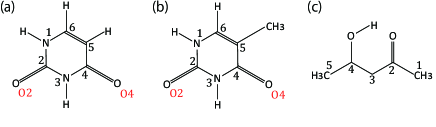
Figure 1: Structures of (a) uracil, (b) thymine, and (c) acetylacetone. Atom numbering follows the IUPAC standard.

Experimental TR-XAS spectra have not been recorded for uracil yet, but its planar symmetry at the Franck-Condon (FC) geometry and its similarities with thymine make it a computationally attractive model system. Experimental TR-XAS data are available at the O K-edge of thymine and at the C K-edge of acetylacetone.

The paper is organized as follows: First, we describe the methodology and computational details. We then compare the results obtained with the CVS-ADC(2), CVS-EOM-CCSD, and TDDFT methods against the experimental ground-state XAS spectra. Feyer et al. (2010); Wolf et al. (2017); Attar et al. (2017); Bhattacherjee et al. (2017) We also compare the computed valence-excitation energies with UV absorption and electron energy loss spectroscopy (EELS, often called electron impact spectroscopy when it is applied to gas-phase molecules). Trajmar (1980) We then present the XAS spectra of the valence-excited states obtained with different CCSD-based protocols and compare them with experimental TR-XAS spectra when available. Wolf et al. (2017); Attar et al. (2017); Bhattacherjee et al. (2017) Finally, we evaluate the performance of MOM-TDDFT.

II Methodology

II.1 Protocols for Computing XAS

We calculated the energies and oscillator strengths for core and valence excitations from the ground states by standard linear-response/equation-of-motion methods: ADC(2), Schirmer (1982); Trofimov and Schirmer (1995); Dreuw and Wormit (2015) EOM-EE-CCSD, Christiansen et al. (1996); Hald, Hättig, and Jørgensen (2000); Bartlett and Musiał (2007); Stanton and Bartlett (1993); Krylov (2008); Bartlett (2012); Coriani et al. (2016) and TDDFT. In the ADC(2) and CCSD calculations of the valence-excited states, we employ the frozen core (fc) approximation. CVS Wenzel, Wormit, and Dreuw (2014); Coriani and Koch (2015); Vidal et al. (2019) was applied to obtain the core-excited states within all methods. Within the fc-CVS-EOM-EE-CCSD framework, Vidal et al. (2019) we explored three different strategies to obtain the excitation energies and oscillator strengths for selected core-valence transitions, as summarized in Fig. 2. In the first one, referred to as standard CVS-EOM-CCSD, we assume that the final core-excited states belong to the set of excited states that can be reached by core excitation from the ground states (see Fig. 2, top panel). Accordingly, we use the HF Slater determinant, representing the ground state ($|\Phi_{0}\rangle$) as the reference ($|\Phi_{\mathrm{ref}}\rangle$) for the CCSD calculation; the (initial) valence-excited and (final) core-excited states are then computed with EOM-EE-CCSD and fc-CVS-EOM-EE-CCSD, respectively. The transition energies for core-valence excitations are subsequently computed as the energy differences between the final core states and the initial valence state. The oscillator strengths for the transitions between the two excited states are obtained from the transition moments between the EOM states, according to EOM-EE theory. Stanton and Bartlett (1993); Bartlett and Musiał (2007); Vidal et al. (2019) In this approach, both the initial and the final states are spin-pure states. However, the final core-hole states that have multiple excitation character with respect to the ground state are either not accessed or described poorly by this approach (the respective configurations are crossed in Fig. 2).

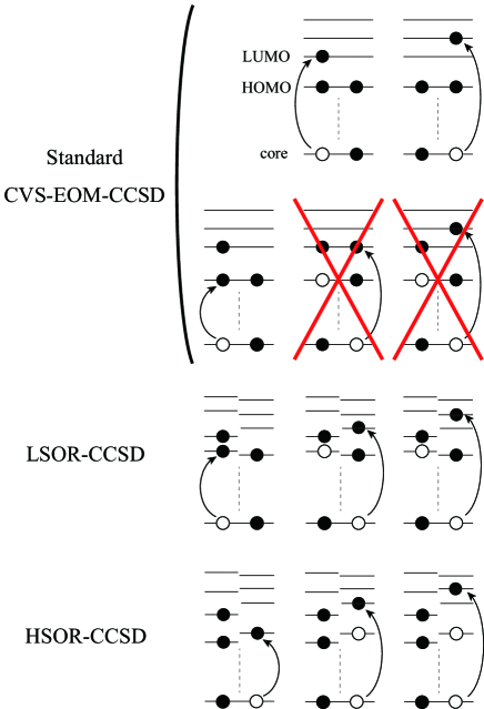
Figure 2: Schematics of the standard CVS-EOM-CCSD, LSOR-CCSD, and HSOR-CCSD protocols. The crossed configurations are formally doubly excited with respect to the ground-state reference.

In the second approach, named high-spin open-shell reference (HSOR) CCSD, we use as a reference ($|\Phi_{\mathrm{ref}}\rangle$) for the CCSD calculations a high-spin open-shell HF Slater determinant that has the same electronic configuration as the initial singlet valence-excited state to be probed in the XAS step. Tsuru et al. (2019); Vidal, Krylov, and Coriani (2020a, b) This approach is based on the assumption that the exchange interactions, which are responsible for the energy gap between singlets and triplets, cancel out in calculations of the transition energies and oscillator strengths. An attractive feature of this approach is that the reference is spin complete (as opposed to a low-spin open-shell determinant of the same occupation) and that the convergence of the SCF procedure is usually robust. A drawback of this approach is the inability to distinguish between the singlet and triplet states with the same electronic configurations.

In the third approach, we use low-spin (M_s=0) MOM-reference for singlet excited states and high-spin (M_s=1) MOM-reference for triplet excited states. We refer to this approach as low-spin open-shell reference (LSOR) CCSD.

In both HSOR-CCSD and LSOR-CCSD, the calculation begins with an SCF optimization targeting the dominant configuration of the initial valence-excited state by means of the MOM algorithm, and the resulting Slater determinant is then used as the reference $|\Phi_{\mathrm{ref}}\rangle$ in the subsequent CCSD calculation. Core-excitation energies and oscillator strengths from the high-spin and the low-spin references are computed with standard CVS-EOM-EE-CCSD. Such MOM-based CCSD calculations can describe all target core-hole states, provided that they have singly excited character with respect to the chosen reference. Furthermore, in principle, initial valence-excited states of different spin symmetry can be selected. However, in calculations using low-spin open-shell references (LSOR-CCSD states), variational collapse might occur. Moreover, the LSOR-CCSD treatment of singlet excited states suffers from spin contamination, as the underlying open-shell reference is not spin complete (the well known issue of spin-completeness in calculations using open-shell references is discussed in detail in recent review articles. Krylov (2017); Casanova and Krylov (2020))

We note that the HSOR-CCSD ansatz for a spin-singlet excited state is identical to the LSOR-CCSD ansatz of a (M_s = 1) spin-triplet state having the same electronic configuration as the spin-singlet excited state (see Fig. 2).

In addition to the three CCSD-based protocols described above, we also considered MOM-TDDFT, which is often used for simulation of the TR-NEXAFS spectra. Attar et al. (2017); Bhattacherjee et al. (2017); Northey et al. (2020) We employed the B3LYP xc-functional, Becke (1993) as in Refs. 20; 22; 47.

II.2 Computational Details

The equilibrium geometry of uracil was optimized at the MP2/cc-pVTZ level. The equilibrium geometries of thymine and acetylacetone were taken from the literature; Wolf et al. (2017); Faber et al. (2019) they were optimized at the CCSD(T)/aug-cc-pVDZ and CCSD/aug-cc-pVDZ level, respectively. These structures represent the molecules at the Franck-Condon (FC) points. The structures of the T₁($\pi\pi^{\ast}$) and S₁(n$\pi^{\ast}$) states of acetylacetone, and of the S₁(n$\pi^{\ast}$) state of thymine were optimized at the EOM-EE-CCSD/aug-cc-pVDZ level. Faber et al. (2019)

We calculated near-edge X-ray absorption fine structure (NEXAFS) of the ground state of all three molecules using CVS-ADC(2), CVS-EOM-CCSD, and TDDFT/B3LYP. The excitation energies of the valence-excited states were calculated with ADC(2), EOM-EE-CCSD, and TDDFT/B3LYP. The XAS spectra of the T₁($\pi\pi^{\ast}$), T₂(n$\pi^{\ast}$), S₁(n$\pi^{\ast}$) and S₂($\pi\pi^{\ast}$) states of uracil were calculated at the FC geometry. We used the FC geometry for all states in order to make a coherent comparison of the MOM-based CCSD methods with the standard CCSD method, and to ensure that the final core-excited states are the same in the ground state XAS and transient state XAS calculations using standard CCSD. The spectra of thymine in the S₁(n$\pi^{\ast}$) state were calculated at the potential energy minimum of the S₁(n$\pi^{\ast}$) state. The spectra of acetylacetone in the T₁($\pi\pi^{\ast}$) and S₂($\pi\pi^{\ast}$) states were calculated at the potential energy minima of the T₁($\pi\pi^{\ast}$) and S₁(n$\pi^{\ast}$) states, respectively. Our choice of geometries for acetylacetone is based on the fact that the S₂($\pi\pi^{\ast}$)-state spectra were measured during wave packet propagation from the S₂($\pi\pi^{\ast}$) minimum (planar) towards the S₁(n$\pi^{\ast}$) minimum (distorted) and the ensemble was in equilibrium when the T₁($\pi\pi^{\ast}$)-state spectra were measured. Bhattacherjee et al. (2017)

The XAS spectra of the valence-excited states were computed with CVS-EOM-CCSD, HSOR-CCSD, and LSOR-CCSD. Pople’s 6-311++G** basis set was used throughout. In each spectrum, the oscillator strengths were convoluted with a Lorentzian function (FWHM = 0.4 eV, unless otherwise specified). We used the natural transition orbitals (NTOs) Luzanov, Sukhorukov, and Umanskii (1976); Martin (2003); Luzanov and Zhikol (2012); Plasser, Wormit, and Dreuw (2014); Plasser et al. (2014b); Bäppler et al. (2014); Mewes et al. (2018); Kimber and Plasser (2020); Krylov (2020) to determine the character of the excited states.

All calculations were carried out with the Q-Chem 5.3 electronic structure package. Shao et al. (2015) The initial guesses [HOMO($\beta$)]¹[LUMO($\alpha$)]¹ and [HOMO($\alpha$)]¹[LUMO($\alpha$)]¹ were used in MOM-SCF for the spin-singlet and triplet states dominated by (HOMO)¹(LUMO)¹ configuration, respectively. The SOMOs of the initial guess in a MOM-SCF process are the canonical orbitals (or the Kohn-Sham orbitals) which resemble the hole and particle NTO of the transition from the ground state to the valence-excited state. One should pay attention to the order of the orbitals obtained in the ground-state SCF, especially when the basis set has diffuse functions. In LSOR-CCSD calculation, the SCF convergence threshold had to be set to $10^{-9}$ Hartree. To ensure convergence to the dominant electronic configuration of the desired electronic state, we used the initial MOM (IMOM) algorithm Barca, Gilbert, and Gill (2018) instead of regular MOM; this is especially important for cases when the desired state belongs to the same irreducible representation as the ground state.

III Results and Discussion

III.1 Ground-State NEXAFS

Fig. 3 shows the O K-edge NEXAFS spectra of uracil in the ground state computed by CVS-EOM-CCSD, CVS-ADC(2), and TDDFT/B3LYP. Table 1 shows NTOs of the core-excited states calculated at the CVS-EOM-CCSD/6-311++G** level, where $\sigma_{K}$ are the singular values for a given NTO pair (their renormalized squares give the weights of the respective configurations in the transition). Luzanov, Sukhorukov, and Umanskii (1976); Martin (2003); Luzanov and Zhikol (2012); Plasser, Wormit, and Dreuw (2014); Plasser et al. (2014b); Bäppler et al. (2014); Mewes et al. (2018); Kimber and Plasser (2020); Krylov (2020) The NTOs for the other two methods are collected in the SI. Panel (d) of Fig. 3 shows the experimental spectrum (digitized from Ref. 105). The experimental spectrum has two main peaks at 531.3 and 532.2 eV, assigned to core excitations to the $\pi^{\ast}$ orbitals from O4 and O2, respectively. Beyond these peaks, the intensity remains low up to 534.4 eV. The next notable spectral feature, attributed to Rydberg excitations, emerges at around 535.7 eV, just before the first core-ionization onset (indicated as IE). The separation of $\sim$0.9 eV between the two main peaks is reproduced at all three levels of theory. The NTO analysis at the CCSD level (cf. Table 1) confirms that the excitation to the 6A" state has Rydberg character and, after the uniform shift, the peak assigned to this excitation falls in the Rydberg region of the experimental spectrum. ADC(2) also yields a 6A" transition of Rydberg character, but it is significantly red-shifted relative to the experiment. No Rydberg transitions are found at the TDDFT level. Only CVS-EOM-CCSD reproduces the separation between the 1A" and the 6A" peaks with reasonable accuracy, 4.91 eV versus 4.4 eV in the experimental spectrum. The shoulder structure of the experimental spectrum in the region between 532.2 and 534.4 eV is attributed to vibrational excitations or shake-up transitions. Stöhr (1992); Rehr et al. (1978)

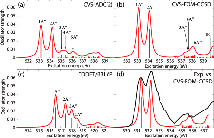
Figure 3: Uracil. Ground-state NEXAFS at the oxygen K-edge calculated with: (a) ADC(2); (b) CVS-EOM-CCSD; (c) TDDFT/B3LYP. The calculated IEs are 539.68 and 539.86 eV (fc-CVS-EOM-IP-CCSD/6-311++G**). In panel (d) the computed spectrum of (b) is shifted by $-$1.8 eV and superposed with the experimental spectrumFeyer et al. (2010) (black curve). Basis set: 6-311++G**.

Table 1: Uracil. CVS-EOM-CCSD/6-311++G** energies, strengths and NTOs of the O_1s core excitations from the ground state at the FC geometry (NTO isosurface is 0.04 for the Rydberg transition and 0.05 for the rest).

Final state	$E^{\mathrm{ex}}$ (eV)	Osc. strength	Hole	$\sigma_{K}^{2}$	Particle
1A"	533.17	0.0367		0.78
2A"	534.13	0.0343		0.79
3A"	537.55	0.0003		0.76
4A"	537.66	0.0004		0.78
6A"	538.08	0.0022		0.82

Fig. 4 shows the ground-state NEXAFS spectra of thymine at the O K-edge. For construction of the theoretical absorption spectra, we used FWHM of 0.6 eV for the Lorentzian convolution function. Panel (d) shows the experimental spectrum (digitized from Ref. 21). Both the experimental and calculated spectra exhibit fine structures, similar to those of uracil. Indeed, the first and second peaks at 531.4 and 532.2 eV of the experimental spectrum were assigned to O_1s-hole states having the same electronic configuration characters as the two lowest-lying O_1s-hole states of uracil. The NTOs of thymine can be found in the SI. Again, only CVS-EOM-CCSD reproduces with reasonable accuracy the Rydberg region after 534 eV. The separation of the two main peaks is well reproduced at all three levels of theory.

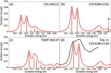
Figure 4: Thymine. Ground-state oxygen K-edge NEXAFS calculated with: (a) ADC(2), (b) CVS-EOM-CCSD, (c) TDDFT/B3LYP. The computed ionization energies (IEs) are 539.67 and 539.73 eV (fc-CVS-EOM-IP-CCSD). In panel (d), the CVS-EOM-CCSD spectrum of (b) is shifted by $-$1.7 eV and superposed with the experimental oneWolf et al. (2017) (black curve). Basis set: 6-311++G**. FWHM of the Lorentzian convolution function is 0.6 eV.

Fig. 5 shows the C K-edge ground-state NEXAFS spectra of acetylacetone; the NTOs of the core excitations obtained at the CVS-EOM-CCSD/6-311++G** level are collected in Table 2. The experimental spectrum, plotted in panel (d) of Fig. 5, was digitized from Ref. 22. Table 2 shows that the first three core excitations are dominated by the transitions to the LUMO from the 1$s$ orbitals of the carbon atoms C2, C3, and C4. Transition from the central carbon atom, C3, appears as the first relatively weak peak at 284.4 eV. We note that acetylacetone may exhibit keto–enol tautomerism. In the keto form, atoms C2 and C4 are equivalent. Therefore, transitions from these carbon atoms appear as quasi-degenerate main peaks at $\approx$286.6 eV. The region around 288.2 eV is attributed to Rydberg transitions. The $\sim$2 eV separation between the first peak and the main peak due to the two quasi-degenerate transitions is well reproduced by ADC(2) and TDDFT/B3LYP, and slightly underestimated by CVS-EOM-CCSD (1.6 eV). On the other hand, the separation of $\sim$1.6 eV between the main peak and the Rydberg resonance region is accurately reproduced only by CVS-EOM-CCSD.

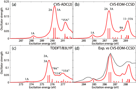
Figure 5: Acetylacetone. Ground-state NEXAFS at carbon K-edge calculated with: (a) ADC(2); (b) CVS-EOM-CCSD; (c) TDDFT/B3LYP. The ionization energies (IEs) are 291.12, 291.88, 292.11, 294.10, and 294.56 eV (fc-CVS-EOM-IP-CCSD). In panel (d), the computational result of (b) is shifted by $-0.9$ eV and superposed with the experimental spectrumBhattacherjee et al. (2017) (black curve). Basis set: 6-311++G**.

Table 2: Acetylacetone. CVS-EOM-CCSD/6-311++G** NTOs of the C_1s core excitations from the ground state at the FC geometry (NTO isosurface is 0.03 for the Rydberg transition and 0.05 for the rest).

Final state	$E^{\mathrm{ex}}$ (eV)	Osc. strength	Hole	$\sigma_{K}^{2}$	Particle
1A	285.88	0.0133		0.76
2A	287.36	0.0671		0.82
3A	287.53	0.0673		0.81
9A	288.63	0.0213		0.79
11A	289.13	0.0202		0.82
13A	289.27	0.0205		0.83
14A	289.28	0.0175		0.82
15A	289.30	0.0174		0.81

The results for the three considered molecules illustrate that CVS-EOM-CCSD describes well the entire pre-edge region of the NEXAFS spectrum. CVS-ADC(2) and TDDFT/B3LYP describe well the core excitations to the LUMO and LUMO+1 (apart from an overall systematic shift), but generally fail to describe the transitions at higher excitation energies.

III.2 Valence-Excited States

Table 3 shows the excitation energies of the two lowest triplet states, the three lowest singlet states, plus the S₅($\pi\pi^{\ast}$) state of uracil, calculated at the FC geometry, along with the values derived from the EELS Chernyshova et al. (2012) and UV absorption experiments. Clark, Peschel, and Tinoco (1965) The EOM-EE-CCSD/6-311++G** NTOs are collected in Table 4 and the NTOs for other methods are given in the SI. We refer to Ref. 125 for an extensive benchmark study of the one-photon absorption and excited-state absorption of uracil.

In EELS, the excited states are probed by measuring the kinetic energy change of a beam of electrons after inelastic collision with the probed molecular sample. Trajmar (1980) In the limit of high incident energy or small scattering angle, the transition amplitude takes a dipole form and the selection rules are same as those of UV-Vis absorption. Otherwise, the selection rules are different and optically dark states can be detected. Furthermore, spin-orbit coupling enables excitation into triplet states. Assignment of the EELS spectral signatures is based on theoretical calculations. Note that excitation energies obtained with EELS may be blue-shifted compared to those from UV-Vis absorption due to momentum transfer between the probing electrons and the probed molecule.

EOM-EE-CCSD excitation energies for all valence states of uracil agree well with the experimental values from EELS. Both the EOM-EE-CCSD and EELS values slightly overestimate the UV-Vis results. For the two triplet states and the S₁(A^′′,n$\pi^{\ast}$) and S₂(A^′,$\pi\pi^{\ast}$) states, ADC(2) also gives fairly accurate excitation energies. ADC(2)-x, on the other hand, seems unbalanced for the valence excitations (regardless of the basis set). The TDDFT/B3LYP excitation energies are red-shifted with respect to the EELS values, but the energy differences between the T₁(A^′, $\pi\pi^{\ast}$), T₂(A^′′, n$\pi^{\ast}$), S₁(A^′′, n$\pi^{\ast}$), and S₂(A^′, $\pi\pi^{\ast}$) states are in reasonable agreement with the corresponding experimentally derived values.

Table 3: Uracil. Excitation energies (eV) at the FC geometry and comparison with experimental values from EELS Chernyshova et al. (2012) and UV absorption spectroscopy. Clark, Peschel, and Tinoco (1965)

	ADC(2)	ADC(2)-x	EOM-CCSD	TDDFT	EELS	UV
T1($\pi\pi^{\ast}$)	3.91	3.36	3.84	3.43	3.75
T2(n$\pi^{\ast}$)	4.47	3.79	4.88	4.27	4.76
S1(n$\pi^{\ast}$)	4.68	3.93	5.15	4.65	5.2
S2($\pi\pi^{\ast}$)	5.40	4.70	5.68	5.19	5.5	5.08
S3($\pi\mathrm{Ryd}$)	5.97	5.39	6.07	5.70	-
S5($\pi\pi^{\ast}$)	6.26	5.32	6.74	5.90	6.54	6.02

Table 4: Uracil. EOM-EE-CCSD/6-311++G** NTOs for the transitions from the ground state to the lowest valence-excited states at the FC geometry (NTO isosurface is 0.05).

Final state	$E^{\mathrm{ex}}$ (eV)	Osc. strength	Hole	$\sigma_{K}^{2}$	Particle
T1(A′,$\pi\pi^{\ast}$)	3.84	-		0.82
T2(A′′,n$\pi^{\ast}$)	4.88	-		0.82
S1(A′′,n$\pi^{\ast}$)	5.15	0.0000		0.81
S2(A’,$\pi\pi^{\ast}$)	5.68	0.2386		0.75
S3(A′′,$\pi\mathrm{Ryd}$)	6.07	0.0027		0.85
S5(A’,$\pi\pi^{\ast}$)	6.74	0.0573		0.73

Table 5 shows the excitation energies of the five lowest triplet and singlet states of thymine, along with the experimental values obtained by EELS. Chernyshova et al. (2013) We did not find literature data for the UV absorption of thymine in the gas phase. The energetic order is based on EOM-EE-CCSD. Here, we reassign the peaks of the EELS spectra Chernyshova et al. (2013) on the basis of the following considerations: $(i)$ optically bright transitions also exhibit strong peaks in the EELS spectra; $(ii)$ the excitation energy of a triplet state is lower than the excitation energy of the singlet state with the same electronic configuration; $(iii)$ the strengths of the transitions to triplet states are smaller than the strengths of the transitions to singlet states; $(iv)$ among the excitations enabled by spin-orbit coupling, $\pi\to\pi^{\ast}$ transitions have relatively large transition moment.

Except for T₁($\pi\pi^{\ast}$), the ADC(2) excitation energies are red-shifted relative to EOM-CCSD. As a result, the ADC(2) excitation energies of the states considered here are closest, in absolute values, to the experimental values from Table 5. However, the energy differences between the singlet states (S₁, S₂, S₄, and S₅) are much better reproduced by EOM-CCSD. TDDFT/B3LYP accurately reproduces the excitation energies of the T₂(n$\pi^{\ast}$), S₁(n$\pi^{\ast}$), and S₂($\pi\pi^{\ast}$) states.

Table 5: Thymine. Excitation energies (eV) at the FC geometry compared with the experimental values from EELS. Chernyshova et al. (2013) The oscillator strengths are from EOM-EE-CCSD, and used for the re-assignment.

	ADC(2)	EOM-CCSD	TDDFT	EELS	Osc. strength
T1($\pi\pi^{\ast}$)	3.70	3.63	3.19	3.66	-
T2(n$\pi^{\ast}$)	4.39	4.81	4.25	4.20	-
S1(n$\pi^{\ast}$)	4.60	5.08	4.64	4.61	0.0000
S2($\pi\pi^{\ast}$)	5.18	5.48	4.90	4.96	0.2289
T3($\pi\pi^{\ast}$)	5.27	5.32	4.61	5.41	-
T4($\pi\mathrm{Ryd}$)	5.66	5.76	5.39	-	-
S3($\pi\mathrm{Ryd}$)	5.71	5.82	5.46	-	0.0005
T5($\pi\pi^{\ast}$)	5.87	5.91	5.10	5.75	-
S4(n$\pi^{\ast}$)	5.95	6.45	5.72	5.96	0.0000
S5($\pi\pi^{\ast}$)	6.15	6.63	5.87	6.17	0.0679

Table 6 shows the excitation energies of the two lowest triplet and singlet states, and the lowest Rydberg states of acetylacetone, along with the experimental values obtained from EELS Walzl, Xavier, and Kuppermann (1987) and UV absorption Nakanishi, Morita, and Nagakura (1977) (the exact state ordering of states in the singlet Rydberg manifold is unknown). Table 7 shows the NTOs obtained at the EOM-EE-CCSD/6-311++G** level. Remarkably, for this molecule the excitation energies from EELS agree well with those from UV absorption. Note that the EELS spectra of acetylacetone were recorded with incident electron energies of 25 and 100 eV, Walzl, Xavier, and Kuppermann (1987) whereas those for uracil Chernyshova et al. (2012) were obtained with 0–8.0 eV. The higher incident electron energies reduce the effective acceptance angle of the electrons, which may hinder the detection of electrons that have undergone momentum transfer. The transitions to the T₁($\pi\pi^{\ast}$) and T₂(n$\pi^{\ast}$) states appeared only with the 25 eV incident electron energy and a scattering angle of 90°  (see Fig. 3 of Ref. 127). The peaks were broad and, furthermore, an order of magnitude less intense than the S${}_{0}\to~{}$S₂($\pi\pi^{\ast}$) transition. Consequently, it is difficult to resolve the excitation energies of T₁($\pi\pi^{\ast}$) and T₂(n$\pi^{\ast}$). ADC(2) yields the best match with the experimental results for acetylacetone.

Table 6: Acetylacetone. Excitation energies (eV) at the FC geometry compared with the values obtained in EELS Walzl, Xavier, and Kuppermann (1987) and UV absorption spectroscopy. Nakanishi, Morita, and Nagakura (1977)

	ADC(2)	ADC(2)-x	EOM-CCSD	TDDFT	EELS	UV
T1($\pi\pi^{\ast}$)	3.76	3.16	3.69	3.23	3.57?	-
T2(n$\pi^{\ast}$)	3.79	3.13	4.11	3.75	?	-
S1(n$\pi^{\ast}$)	4.03	3.29	4.39	4.18	4.04	4.2
S2($\pi\pi^{\ast}$)	4.96	4.28	5.24	5.08	4.70	4.72
T${}_{3}(\pi\mathrm{Ryd})$	5.91	5.45	6.02	5.66	5.52	-
S${}_{3?}(\pi\mathrm{Ryd})$	5.98	5.53	6.13	5.72	5.84	5.85
S${}_{5?}(\pi\mathrm{Ryd})$	6.87	6.30	7.06	6.64	6.52	6.61

Table 7: Acetylacetone. EOM-EE-CCSD/6-311++G** NTOs of the excitations from the ground state to the lowest-lying valence-excited states at the FC geometry (NTO isosurface is 0.03 for the Rydberg transitions and 0.05 for the rest).

Final state	$E^{\mathrm{ex}}$ (eV)	Osc. strength	Hole	$\sigma_{K}^{2}$	Particle
T1(A’,$\pi\pi^{\ast}$)	3.69	-		0.82
T2(A",n$\pi^{\ast}$)	4.11	-		0.82
S1(A",n$\pi^{\ast}$)	4.39	0.0006		0.81
S2(A’,$\pi\pi^{\ast}$)	5.24	0.3299		0.77
T${}_{3}[\pi\mathrm{Ryd}(s)]$	6.02	-		0.86
S${}_{3?}[\pi\mathrm{Ryd}(s)]$	6.13	0.0072		0.86
S${}_{5?}[\pi\mathrm{Ryd}(p)]$	7.06	0.0571		0.85

These results indicate that the excitation energies of the valence-excited states computed by EOM-EE-CCSD, ADC(2), and TDDFT/B3LYP are equally (in)accurate. Which method yields the best match with experiment depends on the molecule.

III.3 Core Excitations from the Valence-Excited States

In Secs. III.1 and III.2, we analyzed two of our three desiderata for a good electronic structure method for TR-XAS—that is, the ability to yield accurate results for ground-state XAS as well as for the valence-excited states involved in the dynamics. In this subsection, we focus on the remaining item, i.e., the ability to yield accurate XAS of valence-excited states.

For uracil, we confirmed that EOM-CCSD and CVS-EOM-CCSD yield fairly accurate results for the valence-excited T₁($\pi\pi^{\ast}$), T₂($\mathrm{n}\pi^{\ast}$), S₁($\mathrm{n}\pi^{\ast}$), and S₂($\pi\pi^{\ast}$) states and for the (final) singlet (O_1s) core-excited states at the FC geometry, respectively. It is thus reasonable to consider the oxygen K-edge XAS spectra of the S₁($\mathrm{n}\pi^{\ast}$) and S₂($\pi\pi^{\ast}$) states of uracil obtained from CVS-EOM-CCSD as our reference, even though CVS-EOM-CCSD only yields the peaks of the core-to-SOMO transitions.

Fig. 6 shows the oxygen K-edge XAS of uracil in the (a) S₁($\mathrm{n}\pi^{\ast}$), (b) S₂($\pi\pi^{\ast}$), (c) T₂($\mathrm{n}\pi^{\ast}$), and (d) T₁($\pi\pi^{\ast}$) states, calculated using CVS-EOM-CCSD (blue curve) and LSOR-CCSD (red curve) at the FC geometry. Note that the HSOR-CCSD spectra of S₁($\mathrm{n}\pi^{\ast}$) and S₂($\pi\pi^{\ast}$) are identical to the LSOR-CCSD spectra for the T₂($\mathrm{n}\pi^{\ast}$) and T₁($\pi\pi^{\ast}$) states, respectively, because their orbital electronic configuration are the same, see Table 4. The ground-state spectrum (green curve) is included in all panels for comparison. The LSOR-CCSD NTOs of the transitions underlying the peaks in the S₁($\mathrm{n}\pi^{\ast}$), S₂($\pi\pi^{\ast}$) and T₁($\pi\pi^{\ast}$) spectra are given in Tabs. 8, 9, and 10, respectively.

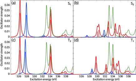
Figure 6: Uracil. Oxygen K-edge NEXAFS of the four lowest-lying valence states: (a) S₁($\mathrm{n}\pi^{\ast}$); (b) S₂($\pi\pi^{\ast}$); (c) T₂($\mathrm{n}\pi^{\ast}$); and (d) T₁($\pi\pi^{\ast}$)]. The blue and red curves correspond to the CVS-EOM-CCSD and LSOR-CCSD results, respectively. Note that the HSOR spectra for S₁ and S₂ are identical to the LSOR-CCSD spectra for T₂ and T₁. Basis set: 6-311++G**. FC geometry. The ground state XAS (green curve) is included for comparison.

Table 8: Uracil. LSOR-CCSD/6-311++G** NTOs of the O_1s core excitations from the S₁ (n$\pi*$) state at the FC geometry (NTO isosurface value is 0.05).

$E^{\mathrm{ex}}$ (eV)	Osc. strength	Spin	Hole	$\sigma_{K}^{2}$	Particle
526.39	0.0451	$\alpha$		0.86
534.26	0.0323	$\alpha$		0.56
		$\beta$		0.23

Table 9: Uracil. LSOR-CCSD/6-311++G** NTOs of the O_1s core excitations from the S₂($\pi\pi^{*}$) state at the FC geometry (NTO isosurface value is 0.05).

$E^{\mathrm{ex}}$ (eV)	Osc. strength	Spin	Hole	$\sigma_{K}^{2}$	Particle
530.16	0.0102	$\alpha$		0.68
530.54	0.0131	$\alpha$		0.67
532.96	0.0186	$\beta$		0.74
534.74	0.0155	$\beta$		0.80
535.70	0.0076	$\alpha$		0.77
535.88	0.0085	$\alpha$		0.76

Table 10: Uracil. LSOR-CCSD/6-311++G** NTOs of the O_1s core excitations from the T₁($\pi\pi^{*}$) state at the FC geometry (NTO isosurface is 0.05).

$E^{\mathrm{ex}}$ (eV)	Osc. strength	Spin	Hole	$\sigma_{K}^{2}$	Particle
529.81	0.0212	$\beta$		0.79
532.39	0.0115	$\beta$		0.78
534.15	0.0187	$\alpha$		0.76
535.09	0.0100	$\alpha$		0.73
535.58	0.0062	$\beta$		0.77
535.61	0.0081	$\beta$		0.72

The CVS-EOM-CCSD spectrum of S₁($\mathrm{n}\pi^{\ast}$) exhibits a relatively intense peak at 528.02 eV, and tiny peaks at 532.40 and 532.52 eV. The intense peak is due to transition from the 1$s$ orbital of O4 to SOMO, which is a lone-pair-type orbital localized on O4. The tiny peak at 532.40 eV is assigned to the transition to SOMO from the 1$s$ orbital of O2, whereas the peak at 532.52 eV is assigned to a transition with multiply excited chatacter. The LSOR-CCSD spectrum exhibits the strong core-to-SOMO transition peak at 526.39 eV, which is red-shifted from the corresponding CVS-EOM-CCSD one by 1.63 eV. As Table 8 shows, the peak at 534.26 eV is due to transition from the 1$s$ orbital of O2 to a $\pi^{\ast}$ orbital, and it corresponds to the second peak in the ground-state spectrum. In the S₁($\mathrm{n}\pi^{\ast}$) XAS spectrum there is no peak corresponding to the first band in the ground-state spectrum, there assigned to the O4 1$s\to\pi^{\ast}$ transition. This suggests that this transition is suppressed by the positive charge localized on O4 in the S₁($\mathrm{n}\pi^{\ast}$) state.

The S₁($\mathrm{n}\pi^{\ast}$) state from LSOR-CCSD is spin-contaminated, with $\langle S^{2}\rangle=1.033$. The spectra of S₁($\mathrm{n}\pi^{\ast}$) yielded by LSOR-CCSD [panel (a)] and by HSOR-CCSD [panel (c)] are almost identical. This is not too surprising, as the spectra of S₁($\mathrm{n}\pi^{\ast}$) and T₂($\mathrm{n}\pi^{\ast}$) from CVS-EOM-CCSD are also almost identical. This is probably a consequence of small exchange interactions in the two states (the singlet and the triplet), due to negligible spatial overlap between the lone pair (n) and $\pi^{\ast}$ orbitals.

In the CVS-EOM-CCSD spectrum of S₂($\pi\pi^{\ast}$), see panel (b), the peaks due to the core-to-SOMO ($\pi$) transitions from O4 and O2 occur at 527.50 and 531.87 eV, respectively. The additional peak at 531.99 eV is assigned to a transition with multiple electronic excitation. In the LSOR-CCSD spectrum, the core-to-SOMO peaks appear at 530.16 and 530.54 eV, respectively.

As shown in Table 9, we assign the peaks at 532.96 and 534.74 eV in the LSOR-CCSD spectrum to transitions from the 1$s$ orbitals of the two oxygens to the $\pi^{\ast}$ orbital, which is half occupied in S₂($\pi\pi^{\ast}$). The NTO analysis reveals that they correspond to the first and second peak of the ground-state spectrum. Note that $\langle S^{2}\rangle$ = 1.326 for the S₂($\pi\pi^{\ast}$) state obtained from LSOR-CCSD.

In the HSOR-CCSD spectrum of the S₂($\pi\pi^{\ast}$) state [which is equal to the LSOR-CCSD spectrum of the T₁($\pi\pi^{\ast}$) state in panel (d)], the peaks of the core-to-SOMO ($\pi$) transitions from O4 and O2 appear at 529.81 and 532.39 eV, respectively (see Table 10). They are followed by transitions to the half-occupied $\pi^{\ast}$ orbital at 534.15 and 535.09 eV, respectively. In contrast to what we observed in the S₁($\mathrm{n}\pi^{\ast}$) spectra, the LSOR-CCSD and HSOR-CCSD spectra of the S₂($\pi\pi^{\ast}$) state are qualitatively different. This can be explained, again, in terms of importance of the exchange interactions in the initial and final states. On one hand, there is a stabilization of the T₁($\pi\pi^{\ast}$) (initial) state over the S₂($\pi\pi^{\ast}$) state by exchange interaction, as the overlap between the $\pi$ and $\pi^{\ast}$ orbitals is not negligible. The exchange interaction between the strongly localized core-hole orbital and the half-occupied valence/virtual orbital in the final core-excited state, on the other hand, is expected to be small.

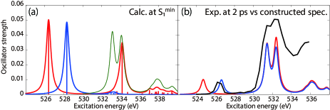
Figure 7: Thymine. (a) Oxygen K-edge NEXAFS in the S₁(n$\pi^{\ast}$) state at its potential energy minimum. Blue: CVS-EOM-CCSD. Red: LSOR-CCSD. Thin green line: ground-state spectrum at the FC geometry. (b) Thick black: Experimental spectrum at the delay time of 2 ps.Wolf et al. (2017) Blue: computational spectrum made from the blue and green curves of (a), shifted by $-$1.7 eV. Red: computational spectrum made from the red and green curves of (a), shifted by $-$1.7 eV. The blue and red curves from (a) were scaled by 0.2 in (b). The ground-state spectrum from (a) was scaled by 0.8 in (b). FWHM of the Lorentzian convolution function is 0.6 eV.

To evaluate the accuracy of the excited-state XAS spectra from CVS-EOM-CCSD and LSOR-CCSD, we also calculated the XAS spectra of the S₁(n$\pi^{\ast}$) state of thymine at the potential energy minimum of S₁(n$\pi^{\ast}$), see panel (a) of Fig. 7. For construction of the surface cut of the theoretical absorption spectra, we chose FWHM of 0.6 eV for the Lorentzian convolution function. Panel (b) shows the spectra of S₁(n$\pi^{\ast}$) multiplied by 0.2 and added to the ground-state spectrum multiplied by 0.8. These factors 0.2 and 0.8 were chosen for the best fit with the experimental spectrum. A surface cut of the experimental TR-NEXAFS spectrum at the delay time of 2 ps Wolf et al. (2017) is also shown in panel (b) of Fig. 7. The reconstructed computational spectra are shifted by $-$1.7 eV. In the experimental spectrum, the core-to-SOMO transition peak occurs at 526.4 eV. In the reconstructed theoretical spectrum, the core-to-SOMO transition peaks appear at 526.62 and 524.70 eV, for CVS-EOM-CCSD and LSOR-CCSD, respectively. Thus, the CVS-EOM-CCSD superposed spectrum agrees slightly better with experiment than the LSOR-CCSD spectrum. Nonetheless, the accuracy of the LSOR-CCSD spectrum is quite reasonable, as compared with the experimental spectrum.

Due to the lack of experimental data, not much can be said about the accuracy of CVS-EOM-CCSD and LSOR-CCSD/HSOR-CCSD for core excitations from a triplet excited state in uracil and thymine. Furthermore, we are unable to unambiguously clarify, using uracil and thymine as model system, which of the two methods, LSOR-CCSD or HSOR-CCSD, should be considered more reliable when they give qualitatively different spectra for the singlet excited states.

Therefore, we turn our attention to the carbon K-edge spectra of acetylacetone and show, in Fig. 8, the spectra obtained using CVS-EOM-CCSD (blue), LSOR-CCSD (red), and HSOR-CCSD (magenta) for the T₁($\pi\pi^{\ast}$) [panel (a)] and S₂($\pi\pi^{\ast}$) [panel (b)] states. The T₁($\pi\pi^{\ast}$) spectra were obtained at the potential energy minimum of T₁($\pi\pi^{\ast}$). The spectra of S₂($\pi\pi^{\ast}$) were calculated at the potential energy minimum of the S₁(n$\pi^{\ast}$) state. In doing so, we assume that the nuclear wave packet propagates on the S₂($\pi\pi^{\ast}$) surface toward the potential energy minimum of the S₁(n$\pi^{\ast}$) surface. Note that CVS-EOM-CCSD does not describe all the core excitations from a valence-excited state (see Fig. 2). In panels (c) and (d), the LSOR-CCSD spectra were multiplied by 0.75 and subtracted from the ground-state spectrum, scaled by 0.25, and superposed to the surface cuts of the experimental transient-absorption NEXAFS at delay times 7-10 ps and 120-200 fs, respectively. The calculated transient-absorption spectra were shifted by $-$0.9 eV, i.e. by the same amount as the spectrum of the ground state [see panel (b) of Fig. 5]. For construction of the surface cut of the theoretical transient-absorption spectra, we used FWHM of 0.6 eV for the Lorentzian convolution function. The scaling factors values 0.75 and 0.25 were chosen to yield the best fit with the experimental spectra. The NTOs of the core excitations from T₁($\pi\pi^{\ast}$) and S₂($\pi\pi^{\ast}$) are shown in Tabs. 11 and 12, respectively. In the experimental study, Bhattacherjee et al. (2017) it was concluded that S₂($\pi\pi^{\ast}$) is populated at the shorter time scale, whereas at the longer time scale it is T₁($\pi\pi^{\ast}$) that becomes populated.

The surface cut of the experimental transient-absorption spectra at longer times (7-10 ps) features two peaks at 281.4 and 283.8 eV. In panel (a) of Fig. 8, the CVS-EOM-CCSD spectrum of T₁($\pi\pi^{\ast}$) shows the core-to-SOMO transition peaks at 282.69 and 284.04 eV, whereas the LSOR-CCSD ones appear at 281.76 and 283.94 eV. The LSOR-CCSD spectrum also shows a peak corresponding to a transition from C4 to the half-occupied $\pi^{\ast}$ orbital at 286.96 eV (see Table 11). The separation of 2.4 eV between the two core-to-SOMO peaks in the experiment is well reproduced by LSOR-CCSD. Spin contamination is small, $\langle S^{2}\rangle$=2.004 for the T₁($\pi\pi^{\ast}$) state obtained using LSOR-CCSD. Therefore, it is safe to say that LSOR-CCSD accurately describes core excitations from the low-lying triplet states.

The surface cut of the transient-absorption spectra at shorter times, 120-240 fs, features relatively strong peaks at 284.7, 285.9 and a ground-state bleach at 286.6 eV. The CVS-EOM-CCSD spectrum of the S₂($\pi\pi^{\ast}$) state shows the core-to-SOMO peak at 280.77. The LSOR-CCSD spectrum (red) has core-to-SOMO transition peaks at 281.30 and 283.69 eV, plus the peaks due to the transitions from the core of C2, C4 and C3 to the half-occupied $\pi^{\ast}$ orbital at 285.43, 286.07 and 287.39 eV, respectively (see Table 12). Note that the peaks at 285.43 and 286.07 eV correspond to the main degenerate peaks of the ground-state spectrum, as revealed by inspection of the NTOs. The HSOR-CCSD spectrum (magenta) exhibits the core-to-SOMO transition peaks at 281.99 and 283.17 eV, followed by only one of the quasi-degenerate peaks corresponding to transitions to the half-occupied $\pi^{\ast}$ orbital, at 287.95 eV. Since the experimental surface-cut spectrum does not clearly show the core-to-SOMO transition peaks, it is difficult to assess the accuracy of these peaks as obtained in the calculations. When it comes to the experimental peaks at 284.7 and 285.9 eV, only LSOR-CCSD reproduces them with reasonable accuracy. The experimental peak at 288.4 eV is not reproduced. In the case of acetylacetone, the HSOR-CCSD approximation fails to correctly mimic the spectrum of S₂($\pi\pi^{\ast}$), since it does not give the peaks at 284.7 and 285.9 eV. The differences between LSOR-CCSD and HSOR-CCSD spectra for S₂($\pi\pi^{\ast}$) can be rationalized as done for uracil.

We emphasize that the assignment of the transient absorption signal at shorter time to S₂($\pi\pi^{\ast}$) is based on peaks assigned to transitions to the $\pi^{\ast}$ orbitals (almost degenerate in the ground state), which cannot be described by CVS-EOM-CCSD (see Fig. 2 in Sec. II.1).

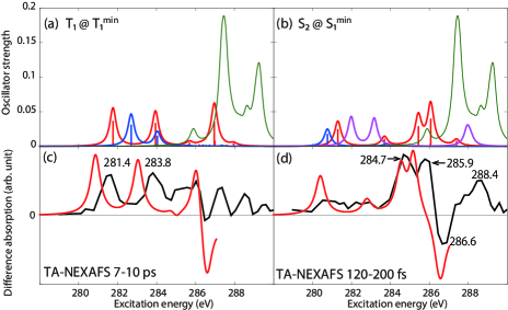
Figure 8: Acetylacetone. Carbon K-edge NEXAFS from the T₁($\pi\pi^{\ast}$) (a) and S₂($\pi\pi^{\ast}$) (b) states. The spectra of T₁($\pi\pi^{\ast}$) were computed at the potential energy minimum of T₁($\pi\pi^{\ast}$). The spectra of S₂($\pi\pi^{\ast}$) were computed at the potential energy minimum of S₁(n$\pi^{\ast}$). Blue: CVS-EOM-CCSD. Red: LSOR-CCSD. Magenta: HSOR-CCSD. Green: ground-state spectrum at the FC geometry. (c), (d) Black: Experimental transient absorption spectra at the delay times of 7-10 ps and 120-200 fs Bhattacherjee et al. (2017), respectively. Red: computational transient absorption spectra made from the red and the green curves of (a) and (b), respectively, shifted by $-$0.9 eV as the spectrum of the ground state [see panel (b) of Fig. 5]. The red curves of panels (a) and (b) were scaled by 0.75 and from these, the green GS spectrum, scaled by 0.25, was subtracted. FWHM of the Lorentzian convolution function is 0.4 eV for panels (a) and (b), 0.6 eV for panels (c) and (d), respectively. Basis set: 6-311++G**.

Table 11: Acetylacetone. LSOR-CCSD/6-311++G** NTOs of the C_1s core excitations from the T₁ state at the potential energy minimum (NTO isosurface is 0.05).

$E^{\mathrm{ex}}$ (eV)	Osc. strength	Spin	Hole	$\sigma_{K}^{2}$	Particle
281.76	0.0347	$\beta$		0.86
283.94	0.0318	$\beta$		0.84
285.69	0.0036	$\beta$		0.72
286.96	0.0334	$\alpha$		0.65
		$\beta$		0.14

Table 12: Acetylacetone. LSOR-CCSD/6-311++G** NTOs of the C_1s core excitations from the S₂ state at the potential energy minimum of S₁ (NTO isosurface is 0.05).

$E^{\mathrm{ex}}$ (eV)	Osc. strength	Spin	Hole	$\sigma_{K}^{2}$	Particle
281.30	0.0228	$\alpha$		0.77
283.69	0.0085	$\alpha$		0.71
285.43	0.0269	$\beta$		0.76
286.07	0.0381	$\beta$		0.76
287.39	0.0057	$\beta$		0.64

On the basis of the above analysis, we conclude that, despite spin contamination, LSOR-CCSD describes the XAS of singlet valence-excited states with reasonable accuracy. LSOR-CCSD could even be used as benchmark for other levels of theory, especially when experimental TR-XAS spectra are not available.

We conclude this section by analyzing the MOM-TDDFT results for the transient absorption. As seen in Secs. III.1 and III.2, ADC(2) and TDDFT/B3LYP yield reasonable results for the lowest-lying core-excited states and for the valence-excited states of interest in the nuclear dynamics. The next question is thus whether MOM-TDDFT/B3LYP can reproduce the main peaks of the time-resolved spectra with reasonable accuracy. We attempt to answer this question by comparing the MOM-TDDFT/B3LYP spectra of thymine and acetylacetone with the surface cuts of the experimental spectra.

The MOM-TDDFT/B3LYP O K-edge NEXAFS spectrum of thymine in the S₁(n$\pi^{\ast}$) state is shown in Fig. 9, panel (a). For construction of the surface cut of the theoretical absorption spectra, we used FWHM of 0.6 eV for the Lorentzian convolution function. A theoretical surface cut spectrum was constructed as sum of the MOM-TDDFT spectrum and the standard TDDFT spectrum of the ground state, scaled by 0.2 and 0.8, respectively. This is shown in panel (b), together with the experimental surface cut spectrum at 2 ps delay.Wolf et al. (2017) The MOM-TDDFT/B3LYP peaks due to the core transitions from O4 and O2 to SOMO (n) are found at 511.82 and 513.50 eV, respectively. The peak corresponding to the first main peak of the ground-state spectrum is missing, and the one corresponding to the second main peak in the GS appears at 517.71 eV. These features are equivalent to what we observed in the LSOR-CCSD case (see Fig. 7). Thus, the separation between the core-to-SOMO peak and the ground-state main peaks is accurately reproduced.

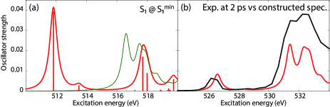
Figure 9: (a) Red: Oxygen K-edge NEXAFS for thymine in the S₁(n$\pi^{\ast}$) state calculated at the MOM-TDDFT/B3LYP/6-311++G** level at the potential energy minimum. Green: Ground-state spectrum. (b) Black: Experimental spectrum at the delay time of 2 ps Wolf et al. (2017), Red: computational spectrum made from the red and the green curves of (a), shifted by $+$14.8 eV. The red curve of (a) was scaled by 0.2. The green curve of (a) was scaled by 0.8. FWHM of the Lorentzian convolution function is 0.6 eV.

Next, we consider the carbon K-edge spectra of acetylacetone in the T₁($\pi\pi^{\ast}$) [at the minimum of T₁($\pi\pi^{\ast}$)] and S₂($\pi\pi^{\ast}$) [at the minimum of S₁(n$\pi^{\ast}$)] states, as obtained from MOM-TDDFT. They are plotted in panels (a) and (b) of Fig. 10, respectively. Surface cuts of the transient-absorption NEXAFS spectra were constructed by subtracting the TDDFT spectrum, scaled by 0.25, with the MOM-TDDFT spectra scaled by 0.75. For this construction, we convoluted the oscillator strengths with a Lorentzian function (FWHM = 0.6 eV), and chose the factors 0.75 and 0.25 for the best fit with the experimental spectra. They are superposed with those from experiment at delay times of 7-10 ps and 120-200 fs in Fig. 10, panels (c) and (d). The MOM-TDDFT spectrum of T₁($\pi\pi^{\ast}$) exhibits the core-to-SOMO transition peaks at 270.88 and 272.41 eV. A peak due to the transition to the half-occupied $\pi^{\ast}$ orbital occurs at 274.16 eV. All peaks observed in the LSOR-CCSD spectrum were also obtained by MOM-TDDFT. The fine structure of the surface-cut transient absorption spectrum is qualitatively reproduced.

The MOM-TDDFT spectrum of S₂($\pi\pi^{\ast}$) exhibits the core-to-SOMO($\pi^{\ast}$) transition peaks at 269.94 and 271.73 eV. The peaks due to the transitions to the half-occupied $\pi^{\ast}$ orbital appear at 274.17 and 274.98 eV. The reconstructed transient-absorption spectrum agrees well with the experimental surface-cut spectrum.

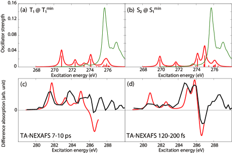
Figure 10: (a), (b) Carbon K-edge NEXAFS for acetylacetone in the T₁($\pi\pi^{\ast}$) and S₂($\pi\pi^{\ast}$) states calculated at the MOM-TDDFT/B3LYP/6-311++G** level at the potential energy minima of T₁($\pi\pi^{\ast}$) and S₁(n$\pi^{\ast}$), respectively. The green curve is the ground-state spectrum. In panels (c) and (d) the experimental transient absorption spectra at delay times of 7-10 ps and 120-200 fs are reported with black lines.Bhattacherjee et al. (2017) In red are the computational transient absorption spectra reconstructed from the red and green curves of panels (a) and (b), respectively, shifted by $+$10.9 eV. The red curves of (a) and (b) were scaled by 0.75, and subtracted from the green curves, which were scaled by 0.25. FWHM of the Lorentzian convolution function is 0.4 eV for panels (a) and (b), 0.6 eV for panels (c) and (d), respectively.

IV Summary and Conclusions

We have analyzed the performance of different single-reference electronic structure methods for excited-state XAS calculations. The analysis was carried out in three steps. First, we compared the results for the ground-state XAS spectra of uracil, thymine, and acetylacetone computed using CVS-ADC(2), CVS-EOM-CCSD, and TDDFT/B3LYP, and with the experimental spectra. Second, we computed the excitation energies of the valence-excited states presumably involved in the dynamics at ADC(2), EOM-EE-CCSD, and TDDFT/B3LYP levels, and compared them with the experimental data from EELS and UV absorption. Third, we analyzed different protocols for the XAS spectra of the lowest-lying valence-excited states based on the CCSD ansatz, namely, regular CVS-EOM-CCSD for transitions between excited states, and EOM-CCSD applied on the excited-state reference state optimized imposing the MOM constraint. The results for thymine and acetylacetone were evaluated by comparison with the experimental time-resolved spectra. Finally, the performance of MOM-TDDFT/B3LYP for TR-XAS was evaluated, again on thymine and acetylacetone, by comparison with the LSOR-CCSD and the experimental spectra.

In the first step, we found that CVS-EOM-CCSD reproduces well the entire pre-edge region of the ground-state XAS spectra. On the other hand, CVS-ADC(2) and TDDFT/B3LYP only describe the lowest-lying core excitations with reasonable accuracy, while the Rydberg region is not captured. In the second step, we observed that EOM-EE-CCSD, ADC(2), and TDDFT/B3LYP treat the valence-excited states with a comparable accuracy.

Among the methods analyzed in the third step, only LSOR-CCSD and MOM-TDDFT can reproduce the entire pre-bleaching region of the excited-state XAS spectra for thymine and acetylacetone, despite spin contamination of the singlet excited states. LSOR-CCSD could be used as the reference when evaluating the performance of other electronic structure methods for excited-state XAS, especially if no experimental spectra are available. For the spectra of the spin-singlet states, CVS-EOM-CCSD yields slightly better core$\to$SOMO positions.

We note that the same procedure can be used to assess the performance of other xc-functional or post-HF methods for TR-XAS calculations. We also note that description of an initial state with the MOM algorithm is reasonably accurate only when the initial state has a single configurational wave-function character. The low computational scaling and reasonable accuracy of MOM-TDDFT makes it rather attractive for the on-the-fly calculation of TR-XAS spectra in the excited-state nuclear dynamics simulations.

Supplementary material

See supplementary material for the NTOs of all core and valence excitations.

Data availability statement

The data that supports the findings of this study are available within the article and its supplementary material.

Conflicts of interest

The authors declare the following competing financial interest(s): A. I. K. is president and part-owner of Q-Chem, Inc.

References

References

- Scherer et al. (1985) N. F. Scherer, J. L. Knee, D. D. Smith, and A. H. Zewail, “Femtosecond photofragment spectroscopy: The reaction ICN CN + I,” J. Phys. Chem. 89, 5141–5143 (1985).
- Young et al. (2018) L. Young, K. Ueda, M. Gühr, P. H. Bucksbaum, M. Simon, S. Mukamel, N. Rohringer, K. C. Prince, C. Masciovecchio, M. Meyer, A. Rudenko, D. Rolles, C. Bostedt, M. Fuchs, D. A. Reis, R. Santra, H. Kapteyn, M. Murnane, H. Ibrahim, F. Légaré, M. Vrakking, M. Isinger, D. Kroon, M. Gisselbrecht, A. L’Huillier, H. J. Wörner, and S. R. Leone, “Roadmap of ultrafast x-ray atomic and molecular physics,” J. Phys. B 51, 032003 (2018).
- Chergui and Collet (2017) M. Chergui and E. Collet, “Photoinduced structural dynamics of molecular systems mapped by time-resolved x-ray methods,” Chem. Rev. 117, 11025–11065 (2017).
- Ueda (2018) K. Ueda, X-ray Free Electron Lasers (MDPI, Basel, Switzerland, 2018).
- Calegari et al. (2016) F. Calegari, G. Sansone, S. Stagira, C. Vozzi, and M. Nisoli, “Advances in attosecond science,” J. Phys. B 49, 062001 (2016).
- Ramasesha, Leone, and Neumark (2016) K. Ramasesha, S. R. Leone, and D. M. Neumark, “Real-time probing of electron dynamics using attosecond time-resolved spectroscopy,” Annu. Rev. Phys. Chem. 67, 41–63 (2016).
- Ischenko, Weber, and Miller (2017) A. A. Ischenko, P. M. Weber, and R. J. D. Miller, “Capturing chemistry in action with electrons: Realization of atomically resolved reaction dynamics,” Chem. Rev. 117, 11066–11124 (2017).
- Villeneuve (2018) D. M. Villeneuve, “Attosecond science,” Contemp. Phys. 59, 47–61 (2018).
- Schuurman and Stolow (2018) M. S. Schuurman and A. Stolow, “Dynamics at conical intersections,” Ann. Rev. Phys. Chem. 69, 427–450 (2018).
- Adachi and Suzuki (2018) S. Adachi and T. Suzuki, “UV-driven harmonic generation for time-resolved photoelectron spectroscopy of polyatomic molecules,” Appl. Sci. 8, 1784 (2018).
- Suzuki (2019) T. Suzuki, “Ultrafast photoelectron spectroscopy of aqueous solutions,” J. Chem. Phys. 151, 090901 (2019).
- Liu et al. (2020) Y. Liu, S. L. Horton, J. Yang, J. P. F. Nunes, X. Shen, T. J. A. Wolf, R. Forbes, C. Cheng, B. Moore, M. Centurion, K. Hegazy, R. Li, M.-F. Lin, A. Stolow, P. Hockett, T. Rozgonyi, P. Marquetand, X. Wang, and T. Weinacht, “Spectroscopic and structural probing of excited-state molecular dynamics with time-resolved photoelectron spectroscopy and ultrafast electron diffraction,” Phys. Rev. X 10, 021016 (2020).
- Glownia et al. (2016) J. M. Glownia, A. Natan, J. P. Cryan, R. Hartsock, M. Kozina, M. P. Minitti, S. Nelson, J. Robinson, T. Sato, T. van Driel, G. Welch, C. Weninger, D. Zhu, and P. H. Bucksbaum, “Self-referenced coherent diffraction x-ray movie of Ångstrom- and femtosecond-scale atomic motion,” Phys. Rev. Lett. 117, 153003 (2016).
- Stankus et al. (2019) B. Stankus, H. Yong, N. Zotev, J. M. Ruddock, D. Bellshaw, T. J. Lane, M. Liang, S. Boutet, S. Carbajo, J. S. Robinson, W. Du, N. Goff, Y. Chang, J. E. Koglin, M. P. Minitti, A. Kirrander, and P. M. Weber, “Ultrafast X-ray scattering reveals vibrational coherence following Rydberg excitation,” Nat. Chem. 11, 716–721 (2019).
- Ruddock et al. (2019) J. M. Ruddock, H. Yong, B. Stankus, W. Du, N. Goff, Y. Chang, A. Odate, A. M. Carrascosa, D. Bellshaw, N. Zotev, M. Liang, S. Carbajo, J. Koglin, J. S. Robinson, S. Boutet, A. Kirrander, M. P. Minitti, and P. M. Weber, “A deep UV trigger for ground-state ring-opening dynamics of 1,3-cyclohexadiene,” Sci. Adv. 5, eaax6625 (2019).
- Stankus et al. (2020) B. Stankus, H. Yong, J. Ruddock, L. Ma, A. M. Carrascosa, N. Goff, S. Boutet, X. Xu, N. Zotev, A. Kirrander, M. P. Minitti, and P. M. Weber, “Advances in ultrafast gas-phase x-ray scattering,” J. Phys. B 53, 234004 (2020).
- Yang et al. (2016) J. Yang, M. Guehr, X. Shen, R. Li, T. Vecchione, R. Coffee, J. Corbett, A. Fry, N. Hartmann, C. Hast, K. Hegazy, K. Jobe, I. Makasyuk, J. Robinson, M. S. Robinson, S. Vetter, S. Weathersby, C. Yoneda, X. Wang, and M. Centurion, “Diffractive imaging of coherent nuclear motion in isolated molecules,” Phys. Rev. Lett. 117, 153002 (2016).
- Stöhr (1992) J. Stöhr, NEXAFS Spectroscopy (Springer-Verlag, Berlin, 1992).
- Pertot et al. (2017) Y. Pertot, C. Schmidt, M. Matthews, A. Chauvet, M. Huppert, V. Svoboda, A. von Conta, A. Tehlar, D. Baykusheva, J.-P. Wolf, and H. J. Wörner, “Time-resolved x-ray absorption spectroscopy with a water window high-harmonic source,” Science 355, 264–267 (2017).
- Attar et al. (2017) A. R. Attar, A. Bhattacherjee, C. D. Pemmaraju, K. Schnorr, K. D. Closser, D. Prendergast, and S. R. Leone, “Femtosecond x-ray spectroscopy of an electrocyclic ring-opening reaction,” Science 356, 54–59 (2017).
- Wolf et al. (2017) T. J. A. Wolf, R. H. Myhre, J. P. Cryan, S. Coriani, R. J. Squibb, A. Battistoni, N. Berrah, C. Bostedt, P. Bucksbaum, G. Coslovich, R. Feifel, K. J. Gaffney, J. Grilj, T. J. Martinez, S. Miyabe, S. P. Moeller, M. Mucke, A. Natan, R. Obaid, T. Osipov, O. Plekan, S. Wang, H. Koch, and M. Gühr, “Probing ultrafast /n internal conversion in organic chromophores via K-edge resonant absorption,” Nat. Commun. 8, 29 (2017).
- Bhattacherjee et al. (2017) A. Bhattacherjee, C. D. Pemmaraju, K. Schnorr, A. R. Attar, and S. R. Leone, “Ultrafast intersystem crossing in acetylacetone via femtosecond X-ray transient absorption at the carbon K-edge,” J. Am. Chem. Soc. 139, 16576–16583 (2017).
- Chen, Zhang, and Shelby (2014) L. X. Chen, X. Zhang, and M. L. Shelby, “Recent advances on ultrafast X-ray spectroscopy in the chemical sciences,” Chem. Sci. 5, 4136–4152 (2014).
- Chergui (2016) M. Chergui, “Time-resolved X-ray spectroscopies of chemical systems: New perspectives,” Struct. Dyn. 3, 031001 (2016).
- Wernet (2019) P. Wernet, “Chemical interactions and dynamics with femtosecond X-ray spectroscopy and the role of X-ray free-electron lasers,” Phil. Trans. R. Soc. A 377, 20170464 (2019).
- Katayama et al. (2019) T. Katayama, T. Northey, W. Gawelda, C. J. Milne, G. Vankó, F. A. Lima, R. Bohinc, Z. Németh, S. Nozawa, T. Sato, D. Khakhulin, J. Szlachetko, T. Togashi, S. Owada, S.-i. Adachi, C. Bressler, M. Yabashi, and T. J. Penfold, “Tracking multiple components of a nuclear wavepacket in photoexcited Cu(I)-phenanthroline complex using ultrafast X-ray spectroscopy,” Nat. Commun. 10, 3606 (2019).
- Norman and Dreuw (2018) P. Norman and A. Dreuw, “Simulating x-ray spectroscopies and calculating core-excited states of molecules,” Chem. Rev. 118, 7208–7248 (2018).
- Bokarev and Kühn (2020) S. I. Bokarev and O. Kühn, “Theoretical x-ray spectroscopy of transition metal compounds,” WIREs Comput. Mol. Sci. 10, e1433 (2020).
- Triguero, Pettersson, and Ågren (1998) L. Triguero, L. G. M. Pettersson, and H. Ågren, “Calculations of near-edge x-ray-absorption spectra of gas-phase and chemisorbed molecules by means of density-functional and transition-potential theory,” Phys. Rev. B 58, 8097–8110 (1998).
- Leetmaa et al. (2010) M. Leetmaa, M. Ljungberg, A. Lyubartsev, A. Nilsson, and L. G. M. Pettersson, “Theoretical approximations to X-ray absorption spectroscopy of liquid water and ice,” J. Electron Spectrosc. Relat. Phenom. 177, 135–157 (2010).
- Vall-llosera et al. (2008) G. Vall-llosera, B. Gao, A. Kivimäki, M. Coreno, J. Álvarez Ruiz, M. de Simone, H. Ågren, and E. Rachlew, “The C 1 and N 1 near edge x-ray absorption fine structure spectra of five azabenzenes in the gas phase,” J. Chem. Phys. 128, 044316 (2008).
- Perera and Urquhart (2017) S. D. Perera and S. G. Urquhart, “Systematic investigation of – interactions in near-edge x-ray fine structure (NEXAFS) spectroscopy of paracyclophanes,” J. Phys. Chem. A 121, 4907–4913 (2017).
- Ehlert, Gühr, and Saalfrank (2018) C. Ehlert, M. Gühr, and P. Saalfrank, “An efficient first principles method for molecular pump-probe NEXAFS spectra: Application to thymine and azobenzene,” J. Chem. Phys. 149, 144112 (2018).
- Ehlert and Klamroth (2020) C. Ehlert and T. Klamroth, “PSIXAS: A Psi4 plugin for efficient simulations of X-ray absorption spectra based on the transition-potential and -Kohn–Sham method,” J. Comput. Chem. 41, 1781–1789 (2020).
- Michelitsch and Reuter (2019) G. S. Michelitsch and K. Reuter, “Efficient simulation of near-edge x-ray absorption fine structure (NEXAFS) in density-functional theory: Comparison of core-level constraining approaches,” J. Chem. Phys. 150, 074104 (2019).
- Dreuw and Head-Gordon (2005) A. Dreuw and M. Head-Gordon, “Single-reference ab initio methods for the calculation of excited states of large molecules,” Chem. Rev. 105, 4009–4037 (2005).
- Luzanov and Zhikol (2012) A. V. Luzanov and O. A. Zhikol, “Excited state structural analysis: TDDFT and related models,” in Practical Aspects of Computational Chemistry, Vol. I, edited by J. Leszczynski and M. K. Shukla (Springer, Heidelberg, Germany, 2012) pp. 415 – 449.
- Laurent and Jacquemin (2013) A. D. Laurent and D. Jacquemin, “TD-DFT benchmarks: A review,” Int. J. Quantum Chem. 113, 2019–2039 (2013).
- Ferré, Filatov, and Huix-Rotllant (2016) N. Ferré, M. Filatov, and M. Huix-Rotllant, eds., Density-Functional Methods for Excited States (Springer, Cham, Switzerland, 2016).
- Stener, Fronzoni, and de Simone (2003) M. Stener, G. Fronzoni, and M. de Simone, “Time dependent density functional theory of core electrons excitations,” Chem. Phys. Lett. 373, 115–123 (2003).
- Besley and Asmuruf (2010) N. A. Besley and F. A. Asmuruf, “Time-dependent density functional theory calculations of the spectroscopy of core electrons,” Phys. Chem. Chem. Phys. 12, 12024–12039 (2010).
- Cederbaum, Domcke, and Schirmer (1980) L. S. Cederbaum, W. Domcke, and J. Schirmer, “Many-body theory of core holes,” Phys. Rev. A 22, 206–222 (1980).
- Besley (2004) N. A. Besley, “Calculation of the electronic spectra of molecules in solution and on surfaces,” Chem. Phys. Lett. 390, 124 – 129 (2004).
- Becke (1993) A. D. Becke, “Density-functional thermochemistry. III. The role of exact exchange,” J. Chem. Phys. 98, 5648–5652 (1993).
- Hait and Head-Gordon (2020a) D. Hait and M. Head-Gordon, “Highly accurate prediction of core spectra of molecules at density functional theory cost: Attaining sub-electronvolt error from a restricted open-shell Kohn–Sham approach,” J. Phys. Chem. Lett. 11, 775–786 (2020a).
- Gilbert, Besley, and Gill (2008) A. T. B. Gilbert, N. A. Besley, and P. M. W. Gill, “Self-consistent field calculations of excited states using the maximum overlap method (MOM),” J. Phys. Chem. A 112, 13164–13171 (2008).
- Northey et al. (2020) T. Northey, J. Norell, A. E. A. Fouda, N. A. Besley, M. Odelius, and T. J. Penfold, “Ultrafast nonadiabatic dynamics probed by nitrogen K-edge absorption spectroscopy,” Phys. Chem. Chem. Phys. 22, 2667–2676 (2020).
- Hait and Head-Gordon (2020b) D. Hait and M. Head-Gordon, “Excited state orbital optimization via minimizing the square of the gradient: General approach and application to singly and doubly excited states via density functional theory,” J. Chem. Theory Comput. 16, 1699–1710 (2020b).
- Hait et al. (2020) D. Hait, E. A. Haugen, Z. Yang, K. J. Oosterbaan, S. R. Leone, and M. Head-Gordon, “Accurate prediction of core-level spectra of radicals at density functional theory cost via square gradient minimization and recoupling of mixed configurations,” J. Chem. Phys. 153, 134108 (2020).
- Bartlett and Musiał (2007) R. J. Bartlett and M. Musiał, “Coupled-cluster theory in quantum chemistry,” Rev. Mod. Phys. 79, 291–352 (2007).
- Koch and Jørgensen (1990) H. Koch and P. Jørgensen, “Coupled cluster response functions,” J. Chem. Phys. 93, 3333–3344 (1990).
- Christiansen, Jørgensen, and Hättig (1998) O. Christiansen, P. Jørgensen, and C. Hättig, “Response functions from Fourier component variational perturbation theory applied to a time-averaged quasienergy,” Int. J. Quantum Chem. 68, 1–52 (1998).
- Sneskov and Christiansen (2012) K. Sneskov and O. Christiansen, “Excited state coupled cluster methods,” WIREs Comput. Mol. Sci. 2, 566–584 (2012).
- Stanton and Bartlett (1993) J. F. Stanton and R. J. Bartlett, “The equation of motion coupled-cluster method. A systematic biorthogonal approach to molecular excitation energies, transition probabilities, and excited state properties,” J. Chem. Phys. 98, 7029–7039 (1993).
- Krylov (2008) A. I. Krylov, “Equation-of-Motion Coupled-Cluster Methods for Open-Shell and Electronically Excited Species: The Hitchhiker’s Guide to Fock Space,” Ann. Rev. Phys. Chem. 59, 433–462 (2008).
- Bartlett (2012) R. J. Bartlett, “Coupled-cluster theory and its equation-of-motion extensions,” WIREs Comput. Mol. Sci. 2, 126–138 (2012).
- Coriani et al. (2016) S. Coriani, F. Pawłowski, J. Olsen, and P. Jørgensen, “Molecular response properties in equation of motion coupled cluster theory: A time-dependent perspective,” J. Chem. Phys. 144, 024102 (2016).
- Coriani and Koch (2015) S. Coriani and H. Koch, “Communication: X-ray absorption spectra and core-ionization potentials within a core-valence separated coupled cluster framework,” J. Chem. Phys. 143, 181103 (2015).
- Vidal et al. (2019) M. L. Vidal, X. Feng, E. Epifanovsky, A. I. Krylov, and S. Coriani, “New and efficient equation-of-motion coupled-cluster framework for core-excited and core-ionized states,” J. Chem. Theory Comput. 15, 3117–3133 (2019).
- Tsuru et al. (2019) S. Tsuru, M. L. Vidal, M. Pápai, A. I. Krylov, K. B. Møller, and S. Coriani, “Time-resolved near-edge X-ray absorption fine structure of pyrazine from electronic structure and nuclear wave packet dynamics simulations,” J. Chem. Phys. 151, 124114 (2019).
- Faber et al. (2019) R. Faber, E. F. Kjønstad, H. Koch, and S. Coriani, “Spin adapted implementation of EOM-CCSD for triplet excited states: Probing intersystem crossings of acetylacetone at the carbon and oxygen K-edges,” J. Chem. Phys. 151, 144107 (2019).
- Nanda et al. (2020) K. D. Nanda, M. L. Vidal, R. Faber, S. Coriani, and A. I. Krylov, “How to stay out of trouble in RIXS calculations within the equation-of-motion coupled-cluster damped response theory? Safe hitchhiking in the excitation manifold by means of core-valence separation,” Phys. Chem. Chem. Phys. 22, 2629–2641 (2020).
- Faber and Coriani (2020) R. Faber and S. Coriani, “Core–valence-separated coupled-cluster-singles-and-doubles complex-polarization-propagator approach to X-ray spectroscopies,” Phys. Chem. Chem. Phys. 22, 2642–2647 (2020).
- Vidal, Krylov, and Coriani (2020a) M. L. Vidal, A. I. Krylov, and S. Coriani, “Dyson orbitals within the fc-CVS-EOM-CCSD framework: theory and application to X-ray photoelectron spectroscopy of ground and excited states,” Phys. Chem. Chem. Phys. 22, 2693–2703 (2020a).
- Vidal et al. (2020a) M. L. Vidal, P. Pokhilko, A. I. Krylov, and S. Coriani, “Equation-of-Motion Coupled-Cluster Theory to Model L-Edge X-ray Absorption and Photoelectron Spectra,” J. Phys. Chem. Lett. 11, 8314–8321 (2020a).
- Coriani et al. (2012) S. Coriani, O. Christiansen, T. Fransson, and P. Norman, “Coupled-Cluster Response Theory for Near-Edge X-Ray-Absorption Fine Structure of Atoms and Molecules,” Phys. Rev. A 85, 022507 (2012).
- Frati et al. (2019) F. Frati, F. de Groot, J. Cerezo, F. Santoro, L. Cheng, R. Faber, and S. Coriani, “Coupled cluster study of the x-ray absorption spectra of formaldehyde derivatives at the oxygen, carbon, and fluorine K-edges,” J. Chem. Phys. 151, 064107 (2019).
- Carbone et al. (2019) J. P. Carbone, L. Cheng, R. H. Myhre, D. Matthews, H. Koch, and S. Coriani, “An analysis of the performance of coupled cluster methods for K-edge core excitations and ionizations using standard basis sets,” Adv. Quant. Chem. 79, 241–261 (2019).
- Peng et al. (2015) B. Peng, P. J. Lestrange, J. J. Goings, M. Caricato, and X. Li, “Energy-Specific Equation-of-Motion Coupled-Cluster Methods for High-Energy Excited States: Application to -Edge X-Ray Absorption Spectroscopy,” J. Chem. Theory Comput. 11, 4146–4153 (2015).
- Fransson et al. (2013) T. Fransson, S. Coriani, O. Christiansen, and P. Norman, “Carbon x-ray absorption spectra of fluoroethenes and acetone: A study at the coupled cluster, density functional, and static-exchange levels of theory,” J. Chem. Phys. 138, 124311 (2013).
- Sarangi et al. (2020) R. Sarangi, M. L. Vidal, S. Coriani, and A. I. Krylov, “On the basis set selection for calculations of core-level states: different strategies to balance cost and accuracy,” Mol. Phys. 118, e1769872 (2020).
- Tenorio et al. (2019) B. N. C. Tenorio, T. Moitra, M. A. C. Nascimento, A. B. Rocha, and S. Coriani, “Molecular inner-shell photoabsorption/photoionization cross sections at core-valence-separated coupled cluster level: Theory and examples,” J. Chem. Phys. 150, 224104 (2019).
- Moitra et al. (2020) T. Moitra, D. Madsen, O. Christiansen, and S. Coriani, “Vibrationally resolved coupled-cluster x-ray absorption spectra from vibrational configuration interaction anharmonic calculations,” J. Chem. Phys. 153, 234111 (2020).
- Vidal et al. (2020b) M. L. Vidal, M. Epshtein, V. Scutelnic, Z. Yang, T. Xue, S. R. Leone, A. I. Krylov, and S. Coriani, “Interplay of Open-Shell Spin-Coupling and Jahn-Teller Distortion in Benzene Radical Cation Probed by X-ray Spectroscopy,” J. Phys. Chem. A 124, 9532–9541 (2020b).
- Costantini et al. (2019) R. Costantini, R. Faber, A. Cossaro, L. Floreano, A. Verdini, C. Hättig, A. Morgante, S. Coriani, and M. Dell’Angela, “Picosecond timescale tracking of pentacene triplet excitons with chemical sensitivity,” Commun. Phys. 2, 56 (2019).
- Myhre et al. (2018) R. H. Myhre, T. J. A. Wolf, L. Cheng, S. Nandi, S. Coriani, M. Gühr, and H. Koch, “A theoretical and experimental benchmark study of core-excited states in nitrogen,” J. Chem. Phys. 148, 064106 (2018).
- Folkestad et al. (2020) S. D. Folkestad, E. F. Kjønstad, R. H. Myhre, J. H. Andersen, A. Balbi, S. Coriani, T. Giovannini, L. Goletto, T. S. Haugland, A. Hutcheson, I.-M. Høyvik, T. Moitra, A. C. Paul, M. Scavino, A. S. Skeidsvoll, Å. H. Tveten, and H. Koch, “ 1.0: An open source electronic structure program with emphasis on coupled cluster and multilevel methods,” J. Chem. Phys. 152, 184103 (2020).
- Paul, Myhre, and Koch (2021) A. C. Paul, R. H. Myhre, and H. Koch, “New and Efficient Implementation of CC3,” J. Chem. Theory Comput. 17, 117–126 (2021).
- Matthews (2020) D. A. Matthews, “EOM-CC methods with approximate triple excitations applied to core excitation and ionisation energies,” Mol. Phys. 118, e1771448 (2020).
- Peng, Copan, and Sokolov (2019) R. Peng, A. V. Copan, and A. Y. Sokolov, “Simulating x-ray absorption spectra with linear-response density cumulant theory,” J. Phys. Chem. A 123, 1840–1850 (2019).
- Schirmer (1982) J. Schirmer, “Beyond the random-phase approximation: A new approximation scheme for the polarization propagator,” Phys. Rev. A 26, 2395–2416 (1982).
- Dreuw and Wormit (2015) A. Dreuw and M. Wormit, “The algebraic diagrammatic construction scheme for the polarization propagator for the calculation of excited states,” WIREs Comput. Mol. Sci. 5, 82–95 (2015).
- Barth and Schirmer (1985) A. Barth and J. Schirmer, “Theoretical core-level excitation spectra of N2 and CO by a new polarisation propagator method,” J. Phys. B 18, 867–885 (1985).
- Christiansen, Koch, and Jørgensen (1995) O. Christiansen, H. Koch, and P. Jørgensen, “The second-order approximate coupled cluster singles and doubles model CC2,” Chem. Phys. Lett. 243, 409 – 418 (1995).
- Schirmer et al. (1993) J. Schirmer, A. B. Trofimov, K. J. Randall, J. Feldhaus, A. M. Bradshaw, Y. Ma, C. T. Chen, and F. Sette, “-shell excitation of the water, ammonia, and methane molecules using high-resolution photoabsorption spectroscopy,” Phys. Rev. A 47, 1136 (1993).
- Wenzel, Wormit, and Dreuw (2014) J. Wenzel, M. Wormit, and A. Dreuw, “Calculating core-level excitations and x-ray absorption spectra of medium-sized closed-shell molecules with the algebraic-diagrammatic construction scheme for the polarization propagator,” J. Comput. Chem. 35, 1900–1915 (2014).
- Plasser et al. (2014a) F. Plasser, R. Crespo-Otero, M. Pederzoli, J. Pittner, H. Lischka, and M. Barbatti, “Surface hopping dynamics with correlated single-reference methods: 9H-adenine as a case study,” J. Chem. Theory Comput. 10, 1395–1405 (2014a).
- Neville et al. (2016a) S. P. Neville, V. Averbukh, S. Patchkovskii, M. Ruberti, R. Yun, M. Chergui, A. Stolow, and M. S. Schuurman, “Beyond structure: ultrafast X-ray absorption spectroscopy as a probe of non-adiabatic wavepacket dynamics,” Faraday Discuss. 194, 117–145 (2016a).
- Neville et al. (2016b) S. P. Neville, V. Averbukh, M. Ruberti, R. Yun, S. Patchkovskii, M. Chergui, A. Stolow, and M. S. Schuurman, “Excited state X-ray absorption spectroscopy: Probing both electronic and structural dynamics,” J. Chem. Phys. 145, 144307 (2016b).
- Neville et al. (2018) S. P. Neville, M. Chergui, A. Stolow, and M. S. Schuurman, “Ultrafast x-ray spectroscopy of conical intersections,” Phys. Rev. Lett. 120, 243001 (2018).
- Neville and Schuurman (2018) S. P. Neville and M. S. Schuurman, “A general approach for the calculation and characterization of x-ray absorption spectra,” J. Chem. Phys. 149, 154111 (2018).
- Trofimov and Schirmer (1995) A. B. Trofimov and J. Schirmer, “An efficient polarization propagator approach to valence electron excitation spectra,” J. Phys. B 28, 2299–2324 (1995).
- Plekan et al. (2008) O. Plekan, V. Feyer, R. Richter, M. Coreno, M. de Simone, K. C. Prince, A. B. Trofimov, E. V. Gromov, I. L. Zaytseva, and J. Schirmer, “A theoretical and experimental study of the near edge X-ray absorption fine structure (NEXAFS) and X-ray photoelectron spectra (XPS) of nucleobases: Thymine and adenine,” Chem. Phys. 347, 360–375 (2008).
- List et al. (2020) N. H. List, A. L. Dempwolff, A. Dreuw, P. Norman, and T. J. Martínez, “Probing competing relaxation pathways in malonaldehyde with transient X-ray absorption spectroscopy,” Chem. Sci. 11, 4180–4193 (2020).
- Seidu et al. (2019) I. Seidu, S. P. Neville, M. Kleinschmidt, A. Heil, C. M. Marian, and M. S. Schuurman, “The simulation of X-ray absorption spectra from ground and excited electronic states using core-valence separated DFT/MRCI,” J. Chem. Phys. 151, 144104 (2019).
- Lyskov, Kleinschmidt, and Marian (2016) I. Lyskov, M. Kleinschmidt, and C. M. Marian, “Redesign of the DFT/MRCI Hamiltonian,” J. Chem. Phys. 144, 034104 (2016).
- Olsen et al. (1988) J. Olsen, B. O. Roos, P. Jørgensen, and H. J. A. Jensen, “Determinant based configuration interaction algorithms for complete and restricted configuration interaction spaces,” J. Chem. Phys. 89, 2185–2192 (1988).
- Malmqvist, Rendell, and Roos (1990) P. Å. Malmqvist, A. Rendell, and B. O. Roos, “The restricted active space self-consistent-field method, implemented with a split graph unitary group approach,” J. Phys. Chem. 94, 5477–5482 (1990).
- Malmqvist et al. (2008) P. Å. Malmqvist, K. Pierloot, A. R. M. Shahi, C. J. Cramer, and L. Gagliardi, “The restricted active space followed by second-order perturbation theory method: Theory and application to the study of CuO2 and Cu2O2 systems,” J. Chem. Phys. 128, 204109 (2008).
- Delcey et al. (2019) M. G. Delcey, L. K. Sørensen, M. Vacher, R. C. Couto, and M. Lundberg, “Efficient calculations of a large number of highly excited states for multiconfigurational wavefunctions,” J. Comput. Chem. 40, 1789–1799 (2019).
- Hua, Mukamel, and Luo (2019) W. Hua, S. Mukamel, and Y. Luo, “Transient x-ray absorption spectral fingerprints of the S1 dark state in uracil,” J. Phys. Chem. Lett. 10, 7172–7178 (2019).
- Segatta et al. (2020) F. Segatta, A. Nenov, S. Orlandi, A. Arcioni, S. Mukamel, and M. Garavelli, “Exploring the capabilities of optical pump X-ray probe NEXAFS spectroscopy to track photo-induced dynamics mediated by conical intersections,” Faraday Discuss. 221, 245–264 (2020).
- Schweigert and Mukamel (2007) I. V. Schweigert and S. Mukamel, “Coherent ultrafast core-hole correlation spectroscopy: X-ray analogues of multidimensional NMR,” Phys. Rev. Lett. 99, 163001 (2007).
- Lee, Small, and Head-Gordon (2019) J. Lee, D. W. Small, and M. Head-Gordon, “Excited states via coupled cluster theory without equation-of-motion methods: Seeking higher roots with application to doubly excited states and double core hole states,” J. Chem. Phys. 151, 214103 (2019).
- Feyer et al. (2010) V. Feyer, O. Plekan, R. Richter, M. Coreno, M. de Simone, K. C. Prince, A. B. Trofimov, I. L. Zaytseva, and J. Schirmer, “Tautomerism in Cytosine and Uracil: A Theoretical and Experimental X-ray Absorption and Resonant Auger Study,” J. Phys. Chem. A 114, 10270–10276 (2010).
- Trajmar (1980) S. Trajmar, “Electron impact spectroscopy,” Acc. Chem. Res 13, 14–20 (1980).
- Christiansen et al. (1996) O. Christiansen, H. Koch, A. Halkier, P. Jørgensen, T. Helgaker, and A. Sánchez de Merás, “Large-scale calculations of excitation energies in coupled cluster theory: The singlet excited states of benzene,” J. Chem. Phys. 105, 6921–6939 (1996).
- Hald, Hättig, and Jørgensen (2000) K. Hald, C. Hättig, and P. Jørgensen, “Triplet excitation energies in the coupled cluster singles and doubles model using an explicit triplet spin coupled excitation space,” J. Chem. Phys. 113, 7765–7772 (2000).
- Vidal, Krylov, and Coriani (2020b) M. L. Vidal, A. I. Krylov, and S. Coriani, “Correction: Dyson orbitals within the fc-CVS-EOM-CCSD framework: theory and application to X-ray photoelectron spectroscopy of ground and excited states,” Phys. Chem. Chem. Phys. 22, 3744–3747 (2020b).
- Krylov (2017) A. I. Krylov, “The quantum chemistry of open-shell species,” in Reviews in Computational Chemistry (John Wiley & Sons, Ltd, 2017) Chap. 4, pp. 151–224.
- Casanova and Krylov (2020) D. Casanova and A. I. Krylov, “Spin-flip methods in quantum chemistry,” Phys. Chem. Chem. Phys. 22, 4326–4342 (2020).
- Luzanov, Sukhorukov, and Umanskii (1976) A. V. Luzanov, A. A. Sukhorukov, and V. É. Umanskii, “Application of transition density matrix for analysis of excited states,” Theor. Exp. Chem. 10, 354–361 (1976).
- Martin (2003) R. L. Martin, “Natural transition orbitals,” J. Chem. Phys. 118, 4775–4777 (2003).
- Plasser, Wormit, and Dreuw (2014) F. Plasser, M. Wormit, and A. Dreuw, “New tools for the systematic analysis and visualization of electronic excitations. I. Formalism,” J. Chem. Phys. 141, 024106 (2014).
- Plasser et al. (2014b) F. Plasser, S. A. Bäppler, M. Wormit, and A. Dreuw, “New tools for the systematic analysis and visualization of electronic excitations. II. Applications,” J. Chem. Phys. 141, 024107 (2014b).
- Bäppler et al. (2014) S. A. Bäppler, F. Plasser, M. Wormit, and A. Dreuw, “Exciton analysis of many-body wave functions: Bridging the gap between the quasiparticle and molecular orbital pictures,” Phys. Rev. A 90, 052521 (2014).
- Mewes et al. (2018) S. Mewes, F. Plasser, A. I. Krylov, and A. Dreuw, “Benchmarking excited-state calculations using exciton properties,” J. Chem. Theory Comput. 14, 710–725 (2018).
- Kimber and Plasser (2020) P. Kimber and F. Plasser, “Toward an understanding of electronic excitation energies beyond the molecular orbital picture,” Phys. Chem. Chem. Phys. 22, 6058–6080 (2020).
- Krylov (2020) A. I. Krylov, “From orbitals to observables and back,” J. Chem. Phys. 153, 080901 (2020).
- Shao et al. (2015) Y. Shao, Z. Gan, E. Epifanovsky, A. T. B. Gilbert, M. Wormit, J. Kussmann, A. W. Lange, A. Behn, J. Deng, X. Feng, D. Ghosh, M. Goldey, P. R. Horn, L. D. Jacobson, I. Kaliman, R. Z. Khaliullin, T. Kuś, A. Landau, J. Liu, E. I. Proynov, Y. M. Rhee, R. M. Richard, M. A. Rohrdanz, R. P. Steele, E. J. Sundstrom, H. L. Woodcock III, P. M. Zimmerman, D. Zuev, B. Albrecht, E. Alguire, B. Austin, G. J. O. Beran, Y. A. Bernard, E. Berquist, K. Brandhorst, K. B. Bravaya, S. T. Brown, D. Casanova, C.-M. Chang, Y. Chen, S. H. Chien, K. D. Closser, D. L. Crittenden, M. Diedenhofen, R. A. DiStasio Jr., H. Do, A. D. Dutoi, R. G. Edgar, S. Fatehi, L. Fusti-Molnar, A. Ghysels, A. Golubeva-Zadorozhnaya, J. Gomes, M. W. D. Hanson-Heine, P. H. P. Harbach, A. W. Hauser, E. G. Hohenstein, Z. C. Holden, T.-C. Jagau, H. Ji, B. Kaduk, K. Khistyaev, J. Kim, J. Kim, R. A. King, P. Klunzinger, D. Kosenkov, T. Kowalczyk, C. M. Krauter, K. U. Lao, A. D. Laurent, K. V. Lawler, S. V. Levchenko, C. Y. Lin, F. Liu, E. Livshits, R. C. Lochan, A. Luenser, P. Manohar, S. F. Manzer, S.-P. Mao, N. Mardirossian, A. V. Marenich, S. A. Maurer, N. J. Mayhall, E. Neuscamman, C. M. Oana, R. Olivares-Amaya, D. P. O’Neill, J. A. Parkhill, T. M. Perrine, R. Peverati, A. Prociuk, D. R. Rehn, E. Rosta, N. J. Russ, S. M. Sharada, S. Sharma, D. W. Small, A. Sodt, T. Stein, D. Stück, Y.-C. Su, A. J. W. Thom, T. Tsuchimochi, V. Vanovschi, L. Vogt, O. Vydrov, T. Wang, M. A. Watson, J. Wenzel, A. White, C. F. Williams, J. Yang, S. Yeganeh, S. R. Yost, Z.-Q. You, I. Y. Zhang, X. Zhang, Y. Zhao, B. R. Brooks, G. K. L. Chan, D. M. Chipman, C. J. Cramer, W. A. Goddard III, M. S. Gordon, W. J. Hehre, A. Klamt, H. F. Schaefer III, M. W. Schmidt, C. D. Sherrill, D. G. Truhlar, A. Warshel, X. Xu, A. Aspuru-Guzik, R. Baer, A. T. Bell, N. A. Besley, J.-D. Chai, A. Dreuw, B. D. Dunietz, T. R. Furlani, S. R. Gwaltney, C.-P. Hsu, Y. Jung, J. Kong, D. S. Lambrecht, W. Liang, C. Ochsenfeld, V. A. Rassolov, L. V. Slipchenko, J. E. Subotnik, T. Van Voorhis, J. M. Herbert, A. I. Krylov, P. M. W. Gill, and M. Head-Gordon, “Advances in molecular quantum chemistry contained in the q-chem 4 program package,” Mol. Phys. 113, 184–215 (2015).
- Barca, Gilbert, and Gill (2018) G. M. J. Barca, A. T. B. Gilbert, and P. M. W. Gill, “Simple models for difficult electronic excitations,” J. Chem. Theory Comput. 14, 1501–1509 (2018).
- Rehr et al. (1978) J. J. Rehr, E. A. Stern, R. L. Martin, and E. R. Davidson, “Extended x-ray-absorption fine-structure amplitudes—Wave-function relaxation and chemical effects,” Phys. Rev. B 17, 560–565 (1978).
- Chernyshova et al. (2012) I. V. Chernyshova, J. E. Kontros, P. P. Markush, and O. B. Shpenik, “Excitation of lowest electronic states of the uracil molecule by slow electrons,” Opt. Spectrosc. 113, 5–8 (2012).
- Clark, Peschel, and Tinoco (1965) L. B. Clark, G. G. Peschel, and I. Tinoco, “Vapor spectra and heats of vaporization of some purine and pyrimidine bases,” J. Phys. Chem. 69, 3615–3618 (1965).
- Fedotov et al. (2020) D. A. Fedotov, A. C. Paul, P. Posocco, F. Santoro, M. Garavelli, H. Koch, S. Coriani, and R. Improta, “Excited State Absorption of Uracil in the Gas Phase: Mapping the Main Decay Paths by Different Electronic Structure Methods,” (2020), 10.26434/chemrxiv.13176554.v1, accepted in J. Chem. Theory Comput.
- Chernyshova et al. (2013) I. V. Chernyshova, J. E. Kontros, P. P. Markush, and O. B. Shpenik, “Excitations of lowest electronic states of thymine by slow electrons,” Opt. Spectrosc. 115, 645–650 (2013).
- Walzl, Xavier, and Kuppermann (1987) K. N. Walzl, I. M. Xavier, and A. Kuppermann, “Electron-impact spectroscopy of various diketone compounds,” J. Chem. Phys. 86, 6701–6706 (1987).
- Nakanishi, Morita, and Nagakura (1977) H. Nakanishi, H. Morita, and S. Nagakura, “Electronic structures and spectra of the keto and enol forms of acetylacetone,” Bull. Chem. Soc. Jpn. 50, 2255–2261 (1977).