Design Fast Algorithms For Hodgkin-Huxley Neuronal Networks

Abstract

The stiffness of the Hodgkin-Huxley (HH) equations during an action potential (spike) limits the use of large time steps. We observe that the neurons can be evolved independently between spikes, $i.e.,$ different neurons can be evolved with different methods and different time steps. This observation motivates us to design fast algorithms to raise efficiency. We present an adaptive method, an exponential time differencing (ETD) method and a library-based method to deal with the stiff period. All the methods can use time steps one order of magnitude larger than the regular Runge-Kutta methods to raise efficiency while achieving precise statistical properties of the original HH neurons like the largest Lyapunov exponent and mean firing rate. We point out that the ETD and library methods can stably achieve maximum 8 and 10 times of speedup, respectively.

Keywords Fast algorithm; Hodgkin-Huxley networks; Adaptive method; Exponential time differencing method; Library method

1 Introduction

The Hodgkin-Huxley (HH) system [1, 2, 3] is widely used to simulate neuronal networks in computational neuroscience [1, 2, 3]. One of its attractive properties is that it can describe the detailed generation of action potentials realistically, $e.g.$, the spiking of the squid’s giant axon. For numerical simulation in practice, it is generally evolved with simple explicit methods, $\mathit{e.g.}$, the Runge-Kutta scheme, and often with a fixed time step. However, the HH equations become stiff when the HH neuron fires a spike and we have to take a sufficiently small time step to avoid stability problems. The stiffness of HH equations limits its application and as a substitution, the conductance-based integrate-and-fire (I&F) systems are often used in the consideration of efficiency [4, 5, 6, 7] although detailed generation of action potentials in I&F equations are omitted. Therefore, it is meaningful to solve the stiff problem in HH system and design fast algorithms allowing a large time step.

The stiff problem of HH system only occurs during the action potentials which is from the activities of sodium and potassium ions channels. Then a natural idea is to use the adaptive method so that we may use a larger time step outside the stiff period. It works well for a single HH neuron but fails in large-scaled HH networks [8] since there are firing events almost everywhere and the obtained time step in standard adaptive method is very small. One key point we observed is that the neurons interact only at the spike moments, so they can be evolved independently between spikes. Our strategy for the adaptive method is that we use a large time step to evolve the network and split it up into subintervals (small time step) to evolve the neurons that are during the stiff period.

The exponential time differencing (ETD) method [9, 10, 8, 11], proposed for stiff systems, may be another effective and efficiency method for HH equations. The idea of ETD method is that, in each time step, the equations can be written into a dominant linear term and a relatively small residual term. By multiplying an integrating factor, the evolving of HH equations turns to estimate the integral of the residual, which allows a large time step without causing stability problem. The recent study [8] gives a second-order ETD method for a single HH neuron. However, for networks, an efficient and high accurate ETD method has to consider the influence of spike-spike interactions. When evolving a network for one single time step, there may be several neurons firing in the time step. Unknowing when and which neurons will fire, we have to wait until the end of the evolution to consider the spike-induced effects [12, 13, 8], $e.g.$, the change of conductance and membrane potential of postsynaptic neurons. Without a carefully recalibration, the accuracy of the network is only the first-order. We point out that the spike-spike correction procedure introduced in Ref. [7] can solve this problem by iteratively sorting the possible spike times, updating the network to the first one and recomputing all future spikes within the time step. In this Letter, we give a fourth-order ETD method for networks with spike-spike correction.

The above adaptive and ETD methods can achieve high quantitative accuracy of HH neurons like the spike shapes. But sometimes the goal of numerical simulations is to achieve qualitative insight or statistical accuracy, since with uncertainty in the model parameters the HH equations can only approximately describe the biological reality. In this case, we offer a library method [14] to raise efficiency which can avoid the stiff period by treating the HH neuron as an I&F one. The idea of the library method is that once a HH neuron’s membrane potential reaches the threshold, we stop evolving its HH equations and restart after the stiff period with reset values interpolated from a pre-computed high resolution data library. Therefore, we avoid the stiff period and can use a large time step to evolve the HH model. Compared with the original library method in Ref. [14], our library method can significantly simply the way to build the library and improve the precision of library (see section 6).

We use the regular fourth-order Runge-Kutta method (RK4) to compare the performance of the adaptive, ETD and library methods with spike-spike correction procedure included in all the methods. The three advanced methods can use time steps one order of magnitude larger than that in the regular RK4 method while achieving precise statistical properties of the HH model, $e.g.,$ firing rates and chaotic dynamical property. We also give a detailed comparison of efficiency for the given methods. Our numerical results show that the ETD and library methods can achieve stable high times of speedup with a maximum 8 and 10 times, respectively.

The outline of the paper is as follows. In Section 2, we give the equations of the HH model. In Section 3, 4 and 5, we describe the regular RK4, adaptive and ETD method, respectively. In Section 6, we give the details of how to build and use the data library. In Section 7, we give the numerical results. We discuss and conclude in Section 8.

2 The model

The dynamics of the $i$th neuron of a Hodgkin-Huxley (HH) network with $N$ excitatory neurons is governed by

$$C\frac{dV_{i}}{dt}=-(V_{i}-V_{Na})G_{Na}m_{i}^{3}h_{i}-(V_{i}-V_{K})G_{K}n_{i}^{4}-(V_{i}-V_{L})G_{L}+I_{i}^{\textrm{input}}$$ (1)

$$\frac{dz_{i}}{dt}=(1-z_{i})\alpha_{z}(V_{i})-z_{i}\beta_{z}(V_{i})\text{ for }z=m,h\text{ and }n$$ (2)

where $V_{i}$ is the membrane potential, $m_{i}$, $h_{i}$ and $n_{i}$ are gating variables, $V_{Na},V_{K}$ and $V_{L}$ are the reversal potentials for the sodium, potassium and leak currents, respectively, $G_{Na},G_{K}$ and $G_{L}$ are the corresponding maximum conductances. $I_{i}^{\textrm{input}}=-G_{i}(t)(V_{i}-V_{G})$ is the input current with

$$\frac{dG_{i}(t)}{dt}=-\frac{G_{i}(t)}{\sigma_{r}}+H_{i}(t)$$ (3)

$$\frac{dH_{i}(t)}{dt}=-\frac{H_{i}(t)}{\sigma_{d}}+f\sum_{l}\delta(t-s_{il})+\sum_{j\neq i}\sum_{l}S_{ij}\delta(t-\tau_{jl})$$ (4)

where $V_{G}$ is the reversal potential, $G_{i}(t)$ is the conductance, $H_{i}(t)$ is an additional parameter to smooth $G_{i}(t)$, $\sigma_{r}$ and $\sigma_{d}$ are fast rise and slow decay time scale, respectively, and $\delta(\cdot)$ is the Dirac delta function. The second term in Eq. (4) is the feedforward input with magnitude $f$. The input time $s_{il}$ is generated from a Poisson process with rate $\nu$. The third term in Eq. (4) is the synaptic current from synaptic interactions in the network, where $S_{ij}$ is the coupling strength from the $j$th neuron to the $i$th neuron, $\tau_{jl}$ is the $l$th spike time of $j$th neuron. The forms of $\alpha$ and $\beta$ and other model parameters are given in Appendix.

When the voltage $V_{i}$, evolving continuously according to Eqs. (1, 2), reaches the threshold $V^{\textrm{th}}$, we say the $i$th neuron fires a spike at this time. Instantaneously, all its postsynaptic neurons receive this spike and their corresponding parameter $H$ jumps by an appropriate amount $S_{ji}$ for the $j$th neuron. For the sake of simplicity, we mainly consider a homogeneously and randomly connected network with $S_{ij}=A_{ij}S$ where $\mathbf{A}=(A_{ij})$ is the adjacency matrix and $S$ is the coupling strength. But note that the conclusions shown in this paper will not change if we extend the given methods to more complicated networks, $e.g.,$ networks of both excitatory and inhibitory neurons, more realistic connectivity with coupling strength following the typically Log-normal distribution [15, 16].

3 Regular method

We first introduce the regular Runge-Kutta fourth-order scheme (RK4) with fixed time step $\Delta$t to evolve the HH model. For the easy of illustration, we use the vector

$$X_{i}(t)=(V_{i}(t),m_{i}(t),h_{i}(t),n_{i}(t),G_{i}(t),H_{i}(t))$$ (5)

to represent the variables of the $i$th neuron. The neurons interact with each other through the spikes by changing the postsynaptic state of $X$, so it is important to obtain accurate spike sequences, $e.g.,$ at least with an accuracy of fourth-order. We determine the spike times as follows [12, 13]. If neuron $i$ fires in $[t_{n},t_{n+1}]$, $i.e.,$ $V_{i}(t_{n})<V^{\text{th}}$ and $V_{i}(t_{n+1})\geq V^{\text{th}}$, we can use the membrane potential and its derivative at $t=t_{n}$ and $t=t_{n+1}$: $V_{i}(t_{n}),\frac{dV_{i}}{dt}(t_{n}),V_{i}(t_{n+1}),\frac{dV_{i}}{dt}(t_{n+1})$ to perform a cubic Hermite interpolation $p(t)$ to decide the spike time by finding the solution $t_{\text{spike}}$ of $p(t)=V^{\text{th}}$ with $t_{n}<t_{\text{spike}}$$\leq t_{n+1}$. Then the obtained spike time $t_{\text{spike}}$ has an accuracy of fourth-order given that the membrane potential and its derivative has an accuracy of fourth-order as well.

In between spikes, the RK4 method can achieve a fourth-order of accuracy. However, for a spike-containing time step, it requires a careful recalibration of $X$ to account for the spike-spike interaction. For example, consider 2 bidirectionally connected neurons $1$ and $2$. If neuron 1 fires in the time step, then it is necessary to recalibrate $X_{2}$ to achieve an accuracy of fourth-order. If neuron 2 also fires, then $X_{1}$ and spike time of neuron 1 is imprecise and we should recalibrate them. Then again $X_{2}$ and the spike time of neuron 2 is imprecise.

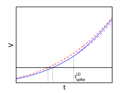
Figure 1: Local error analysis of neuron $1$ for $t_{0}\leq t\leq t_{0}+\Delta t$ . The blue solid line is true membrane potential $v_{1}$, magenta dashdot line is true membrane potential $\tilde{v}_{1}$ without considering the spike from neuron 2 and the red dashed line is the cubic Hermite interpolation $p_{1}$. The solid horizontal line is the threshold and the dotted vertical lines are spike times.

We take the spike-spike correction procedure [7] to solve this problem. The strategy is that we preliminarily evolve neuron 1 and 2 considering only the feedforward input in the time step from $t_{0}$ to $t_{0}+\Delta t$ and decide the spike times $t_{\text{spike}}^{(1)}$ and $t_{\text{spike}}^{(2)}$ by a cubic Hermite interpolation. Suppose that $t_{\text{spike}}^{(1)}<t_{\text{spike}}^{(2)}$. Let $v_{1}(t)$ denote the true membrane potential of neuron 1, $\tilde{v}_{1}(t)$ denote the true membrane potential of neuron 1 without considering the spike of neuron 2 fired at $t_{\text{spike}}^{(2)}$ and $p_{1}(t)$ be the cubit Hermite interpolation for neuron 1 as shown in Fig. 1. Then we have

$$p_{1}(t)-\tilde{v}_{1}(t)=O(\Delta t^{4})\text{ for }t_{0}\leq t\leq t_{0}+\Delta t.$$ (6)

Note that the spike from neuron 2 starts to affect at time $t_{\text{spike}}^{(2)}$, $i.e.$,

$$v_{1}(t)=\tilde{v}_{1}(t)\text{ for }t_{0}\leq t\leq t_{\text{spike}}^{(2)}.$$ (7)

Therefore, the preliminarily computed $t_{\text{spike}}^{(1)}$ indeed has an accuracy of four-order as shown in Fig. 1. Then we can update neuron 1 and 2 from $t_{0}$ to $t_{\text{spike}}^{(1)}$, accept the spike time of neuron 1 at $t_{\text{spike}}^{(1)}$, and evolve them to $t_{0}+\Delta t$ to obtain spike time of neuron 2, $X_{1}(t_{0}+\Delta t)$ and $X_{2}(t_{0}+\Delta t)$ with an accuracy of fourth-order. For large networks, the strategy is the same and detailed algorithm of regular RK4 scheme is given in Algorithm 1.

Input: An initial time $t_{0}$, time step $\Delta t$, feedforward input times $\{s_{il}\}$

Output: $\{X_{i}(t_{0}+\Delta t)\}$ and $\{\tau_{il}\}$(if any fired)

Preliminarily evolve the network from $t_{0}$ to $t_{0}+\Delta t$ to find the first synaptic spike:

for $i=1$ to $N$ do

       Let $M$ denote the total number of feedforward spikes of the $i$th neuron within $[t_{0},t_{0}+\Delta t]$ and sort them into an increasing list $\{T_{m}^{\text{sorted}}\}$. Then we extend this notation such that $T_{0}^{\text{sorted}}:=t_{0}$ and $T_{M+1}^{\text{sorted}}:=t_{0}+\Delta t$.

       for $m=1$ to $M+1$  do

             Advance the equations for the $i$th HH neuron from $T_{m-1}^{\text{sorted}}$ to $T_{m}^{\text{sorted}}$ using the standard RK4 scheme. Then update the conductance $H_{i}(T_{m}^{\text{sorted}})$ by adding $f$.

            

            if $V_{i}(T_{m-1}^{\text{sorted}})<V^{\textrm{th}}$, $V_{i}(T_{m}^{\text{sorted}})\geq V^{\textrm{th}}$ then

                   We know that the $i$th neuron spiked during $[T_{m-1}^{\text{sorted}},T_{m}^{\text{sorted}}]$.

                   Find the spike time $t_{\text{spike}}^{(i)}$ by a cubic Hermite interpolation using the values $V_{i}(T_{m-1}^{\text{sorted}})$, $V_{i}(T_{m}^{\text{sorted}})$, $\frac{dV_{i}}{dt}(T_{m-1}^{\text{sorted}})$ and $\frac{dV_{i}}{dt}(T_{m}^{\text{sorted}})$.

                  

            

      

while $\{t_{\text{spike}}^{(i)}\}$ is non-empty do

       Find the minimum of $\{t_{\text{spike}}^{(i)}\}$, say $t_{\text{spike}}^{(i_{1})}$. Evolve neuron $i_{1}$ to $t_{\text{spike}}^{(i_{1})}$, generate a spike at this moment and update its postsynaptic neurons to $t_{\text{spike}}^{(i_{1})}$. Preliminarily evolve the affected neurons from $t_{\text{spike}}^{(i_{1})}$ to $t_{0}+\Delta t$ to update their spike times $\{t_{\text{spike}}\}$.

We accept $\{X_{i}{(T_{M+1}^{\text{sorted}})}\}$ as the solution $\{X_{i}{(t+\Delta t)}\}$;

Algorithm 1 Regular RK4 algorithm

4 Adaptive method

When a neuron fires a spike, the HH neuron equations are stiff for some milliseconds, denoted by $T^{\textrm{stiff}}$ as shown in Fig. 2. This stiff period requires a sufficiently small time step to avoid stability problem. In the regular RK4 scheme, we use fixed time step, so to satisfy the requirement of stability, we have to use a relatively small time step, $\mathit{e.g.}$, $\Delta t=1/32$ ms. But we may need to simulate the HH model frequently to analyze the system’s behavior with different parameters or evolve the model for a long run time (hours) to obtain precise statistical properties. Therefore, it is important to enlarge the time step as much as possible to raise efficiency.

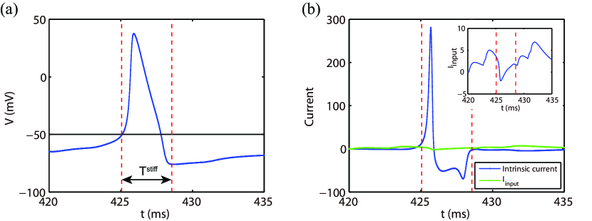
Figure 2: Typical firing event of a single HH neuron. (a) The trajectory of voltage $V$. The black line indicates the threshold $V^{\textrm{th}}$ and the red dotted lines indicate the stiff period. (b) The trajectory of the intrinsic current and input current $I_{i}^{\textrm{input}}$ ($\mu\textrm{A$\cdot$cm}^{-2}$). The intrinsic current is the sum of ionic and leakage currents.

We note that between spikes the neurons do not affect each other and thus can be evolved independently. As shown in Algorithm 1, we induce the spike-spike correction to obtain a high accurate method of fourth-order, $i.e.$, we should split up the time step once a presynaptic neuron fires. Therefore, the neurons are indeed evolved independently in simulation. With this observation, we can design efficient method by reasonably treating the neurons inside the stiff period.

We first introduce our adaptive method. Note that the derivative of voltage is quite small outside the stiff period as shown in Fig. 2(b). Then strategy is that we take a large time step $\Delta t$ to evolve the network. Once a neuron is in the stiff period, the large time step is then split up into small time steps $\Delta t_{S}$, $e.g.,$ with a value of $\Delta t_{S}=1/32$ ms in this Letter, as shown in Fig. 3. For each time step, we still use the standard RK4 scheme to evolve the neurons, so the adaptive method has an accuracy of $O(\Delta t^{4})$. Detailed adaptive algorithm is the same as the Algorithm 1 except that the step 3 in Algorithm 1 should be replaced by the following algorithm.

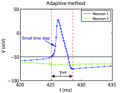
Figure 3: Illustration of the adaptive method for two HH neurons unidirectionally connected from neuron 1 to neuron 2. After neuron 1 fires a spike, it is evolved with a small time step $\Delta t_{S}$ during the stiff period indicated by the stars. The dots indicate the time nodes for the large time step. The green square indicates an update time node due to the synaptic spike from neuron 1.

if The $i$th neuron is outside the stiff period then

       Let $M$ denote the total number of feedforward spikes of the $i$th neuron within $[t_{0},t_{0}+\Delta t]$.

else

       Let $M$ denote the total number of feedforward spikes of the $i$th neuron within $[t_{0},t_{0}+\Delta t]$ and the extra time nodes $t_{0}+\Delta t_{S},t_{0}+2\Delta t_{S},...,t_{0}+k\Delta t_{S}$, $k=[\frac{\Delta t}{\Delta t_{S}}]$ ($[\cdot]$ takes the round-off number).

Sort them into an increasing list $\{T_{m}^{\text{sorted}}\}$ and extend this notation such that $T_{0}^{\text{sorted}}:=t_{0}$ and $T_{M+1}^{\text{sorted}}:=t_{0}+\Delta t$.

Algorithm 2 Adaptive algorithm

5 Exponential time differencing method

We now introduce the exponential time differencing method (ETD) which is proposed for stiff systems [10, 8, 9]. To describe the ETD methods for HH networks, it is more instructive to first consider a simple ordinary differential equation

$$\frac{du}{dt}=F(t,u)$$ (8)

where $F(t,u)$ represents the stiff nonlinear forcing term. For a single time step from $t=t_{k}$ to $t=t_{k+1}=t_{k}+\Delta t$, we rewrite the equation

$$\frac{du}{dt}=au+b+(F(t,u)-au-b)$$ (9)

where $au+b$ is the dominant linear approximation of $F(t,u)$, and $F(t,u)-au-b$ is the residual error. By multiplying Eq. (9) through by the integrating factor $e^{-at}$, we can obtain

$$u(t_{k+1})=u(t_{k})e^{a\Delta t}+e^{a\Delta t}\int_{0}^{\Delta t}e^{-a\tau}\tilde{F}(t_{k}+\tau,u(t_{k}+\tau))d\tau.$$ (10)

where $\tilde{F}(t,u)=F(t,u)-au$. This formula is exact, and the essence of the ETD method is to find a proper way to approximate the integral in this expression, $e.g.,$ approximating $\tilde{F}$ by a polynomial.

Here we give an ETD method with Runge-Kutta fourth-order time stepping (ETD4RK). We write $u_{k}$ and $\tilde{F}_{k}$ for the numerical approximations for $u(t_{k})$ and $\tilde{F}(t_{k},u_{k})$, respectively (We use similar writing in the derivation of ETD4RK method for HH equations). The ETD4RK method is given by

$$a_{k} =u_{k}e^{a\Delta t/2}+\tilde{F}_{k}\frac{e^{a\Delta t/2}-1}{a}$$ (11)

$$b_{k} =u_{k}e^{a\Delta t/2}+\tilde{F}(t_{k}+\Delta t/2,a_{k})\frac{e^{a\Delta t/2}-1}{a}$$ (12)

$$c_{k} =a_{k}e^{a\Delta t/2}+(2\tilde{F}(t_{k}+\Delta t/2,b_{k})-\tilde{F}_{k})\frac{e^{a\Delta t/2}-1}{a}$$ (13)

$$u_{k+1} =u_{k}e^{a\Delta t}+g_{0}\tilde{F}_{k}+g_{1}[\tilde{F}(t_{k}+\Delta t/2,a_{k})+\tilde{F}(t_{k}+\Delta t/2,b_{k})]+g_{2}\tilde{F}(t_{k}+\Delta t,c_{k})$$ (14)

where

$$g_{0} =[-4-a\Delta t+e^{a\Delta t}(4-3a\Delta t+a^{2}\Delta t^{2})]/a^{3}\Delta t^{2}$$

$$g_{1} =2[2+a\Delta t+e^{a\Delta t}(-2+a\Delta t)]/a^{3}\Delta t^{2}$$ (15)

$$g_{2} =[-4-3a\Delta t-a^{2}\Delta t^{2}+e^{a\Delta t}(4-a\Delta t)]/a^{3}\Delta t^{2}$$

The above formula requires an appropriate linear approximation $au+b$ for $F(t,u)$ during the single time step, so that the residual error is relatively small and we can use a large time step to raise efficiency. Note that the variables $V,m,h,$ and $n$ appear linearly in the HH equations (1, 2). Therefore, we can directly apply ETD4RK method to HH system. For the easy of writing, we give the standard ETD4RK method for a single HH neuron to evolve over a single time step from $t=t_{k}$ to $t=t_{k+1}=t_{k}+\Delta t$. The HH equations (1, 2) are rewritten in the form

$$\frac{dz}{dt}=a_{z}z+\tilde{F}_{z}(t,V,m,h,n)\text{ for }z=V,m,h\text{ and }n$$ (16)

where

$$a_{V}=(-G_{Na}m_{k}^{3}h_{k}-G_{K}n_{k}^{4}-G_{L})/C$$ (17)

$$a_{z}=-\alpha_{z}(V_{k})-\beta_{z}(V_{k})\text{ for }z=m,h\text{ and }n$$ (18)

and

$$\tilde{F}_{V}=[-(V-V_{Na})G_{Na}m^{3}h-(V-V_{K})G_{K}n^{4}-(V-V_{L})G_{L}+I^{\textrm{input}}-a_{V}V]/C$$ (19)

$$\tilde{F}_{z}=(1-z)\alpha_{z}(V)-z\beta_{z}(V)-a_{z}z\text{ for }z=m,h\text{ and }n.$$ (20)

The standard ETD4RK method is given by

$$a_{z,k} =z_{k}e^{a_{z}\Delta t/2}+\tilde{F}_{z,k}\frac{e^{a_{z}\Delta t/2}-1}{a_{z}}$$ (21)

$$b_{z,k} =z_{k}e^{a_{z}\Delta t/2}+\tilde{F_{z}}(t_{k}+\Delta t/2,a_{V,k},a_{m,k},a_{h,k},a_{n,k})\frac{e^{a_{z}\Delta t/2}-1}{a_{z}}$$ (22)

$$c_{z,k} =a_{z,k}e^{a_{z}\Delta t/2}+(2\tilde{F}_{z}(t_{k}+\Delta t/2,b_{V,k},b_{m,k},b_{h,k},b_{n,k})-\tilde{F}_{z,k})\frac{e^{a_{z}\Delta t/2}-1}{a_{z}}$$ (23)

$$z_{k+1} =z_{k}e^{a_{z}\Delta t}+g_{z,0}\tilde{F}_{z,k}+g_{z,1}\tilde{F_{z}}(t_{k}+\Delta t/2,a_{V,k},a_{m,k},a_{h,k},a_{n,k})$$ (24)

$$+g_{z,1}\tilde{F}_{z}(t_{k}+\Delta t/2,b_{V,k},b_{m,k},b_{h,k},b_{n,k})+g_{z,2}\tilde{F}_{z}(t_{k}+\Delta t,c_{V,k},c_{m,k},c_{h,k},c_{n,k})$$

for $z=V,m,h$ and $n$. The forms of $g_{z,0},g_{z,1},g_{z,2}$ are the same as given in Eq. (15) except that the term $a$ should be replaced by $a_{z}$.

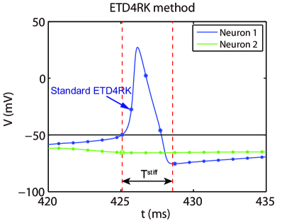
Figure 4: Illustration of the ETD4RK method for two HH neurons unidirectionally connected from neuron 1 to neuron 2. After neuron 1 fires a spike, we use the standard ETD4RK scheme to evolve it during the stiff period indicated by the stars. The dots indicate the time nodes where we use the standard RK4 scheme. The green square indicates an update time node due to the synaptic spike from neuron 1.

Compared with the standard RK4 scheme, the standard ETD4RK scheme requires extra calculation for the linear approximation terms in Eqs. (1, 2). Besides the HH equations are stiff only during an action potential as shown in Fig. 2. Therefore, it is more suitable to design the ETD4RK method for HH networks as following: If a neuron is inside the stiff period, we use the standard ETD4RK scheme to evolve its HH equations, otherwise, we still use the standard RK4 scheme, as shown in Fig. 4. Detailed ETD4RK algorithm is also based on the Algorithm 1 except that the step 5 should be replaced by the following algorithm.

if The $i$th neuron is outside the stiff period then

       Advance the equations for the $i$th HH neuron from $T_{m-1}^{\text{sorted}}$ to $T_{m}^{\text{sorted}}$ using the standard RK4 scheme.

else

       Advance the equations for the $i$th HH neuron from $T_{m-1}^{\text{sorted}}$ to $T_{m}^{\text{sorted}}$ using the standard ETD4RK scheme.

Then update the conductance $H_{i}(T_{m}^{\text{sorted}})$ by adding $f$.

Algorithm 3 ETD4RK algorithm

6 Library method

The introduced adaptive and ETD4RK methods can evolve the HH neuronal networks quite accurately, $e.g.$, they both can capture precise spike shapes. The library method [14] sacrifices the accuracy of the spike shape by treating the HH neuron’s firing event like an I&F neuron. Once a neuron’s membrane potential reaches the threshold $V^{\textrm{th}}$, we stop evolving its $V,m,h,n$ for the following stiff period $T^{\textrm{stiff}}$, and restart with the values interpolated from a pre-computed high resolution library. Thus the library method can achieve the highest efficiency in principle by skipping the stiff period. Besides, it can still capture accurate statistical properties of the HH neuronal networks like the mean firing rates and chaotic dynamics.

6.1 Build the library

We first describe how to build the library in detail. When a neuron’s membrane potential reaches the threshold $V^{\textrm{th}}$, we record the values $I^{\textrm{input}},m,h,n$ and denote them by $I^{\textrm{th}},m^{\textrm{th}},h^{\textrm{th}},n^{\textrm{th}}$, respectively. If we know the exact trajectory of $I^{\textrm{input}}$ for the following stiff period $T^{\textrm{stiff}}$, we can use a sufficiently small time step to evolve the Eqs. (1, 2) for $T^{\textrm{stiff}}$ with initial values $V^{\textrm{th}},m^{\textrm{th}},h^{\textrm{th}},n^{\textrm{th}}$ to obtain high resolution trajectories of $V,m,h,n$. The values at the end of the stiff period are like the reset values in I&F neurons and are denoted by $V^{\textrm{re}},m^{\textrm{re}},h^{\textrm{re}},n^{\textrm{re}}$.

However it is impossible to obtain the exact trajectory of $I^{\textrm{input}}$ without knowing the feedforward and synaptic spike information. As shown in Fig. 2(b), $I^{\textrm{input}}$ varies during the stiff period with peak value in the range of $O(5)$ $\mu\textrm{A$\cdot$cm}^{-2}$, while the intrinsic current, the sum of ionic and leakage current, is about 30 $\mu\textrm{A$\cdot$cm}^{-2}$ at the spike time, and quickly rises to the peak value about 250 $\mu\textrm{A$\cdot$cm}^{-2}$, then stays at $O(-50)$ $\mu\textrm{A$\cdot$cm}^{-2}$ in the remaining stiff period. Therefore, the intrinsic current is dominant in the stiff period. With this observation, we take $I^{\textrm{input}}$ as constant throughout the whole stiff period when we build the library. We emphasize that this is the only assumption made in the library method. Then, given a suite of $I^{\textrm{th}},m^{\textrm{th}},h^{\textrm{th}},n^{\textrm{th}}$, we can obtain the corresponding suite of $V^{\textrm{re}},m^{\textrm{re}},h^{\textrm{re}},n^{\textrm{re}}$.

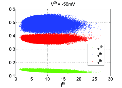
Figure 5: The ranges of values $I^{\textrm{th}},m^{\textrm{th}},h^{\textrm{th}},n^{\textrm{th}}$.

When building the library, we choose $N_{I},N_{m},N_{h},N_{n}$ different values of $I^{\textrm{th}},m^{\textrm{th}},h^{\textrm{th}},n^{\textrm{th}}$, respectively, equally distributed in their ranges as shown in Fig. 5. For each suite of $I^{\textrm{th}},m^{\textrm{th}},h^{\textrm{th}},n^{\textrm{th}}$, we evolve the Eqs. (1, 2) for a time interval of $T^{\textrm{stiff}}$ to obtain $V^{\textrm{re}},m^{\textrm{re}},h^{\textrm{re}},n^{\textrm{re}}$ with RK4 method with a sufficiently small time step, $\mathit{e.g.}$, $\Delta t=2^{-16}$ ms. Note that we should take $I^{\textrm{input}}=I^{\textrm{th}}$ throughout the whole time interval $T^{\textrm{stiff}}$. The library is built with a total size of $8N_{I}N_{m}N_{h}N_{n}$. In our simulation, we take the ranges $[0,50]$ $\mu\textrm{A$\cdot$cm}^{-2}$, $[0,0.3]$, $[0.2,0.6]$ and $[0.3,0.6]$ for $I^{\textrm{th}},m^{\textrm{th}},h^{\textrm{th}},n^{\textrm{th}}$ respectively that can cover almost all possible situations and take sample numbers $N_{I}=21,N_{m}=16,N_{h}=21,N_{n}=16$ which can make the library quite accurate. The library occupies only 6.89 megabyte in binary form and is quite small for today’s computers.

One key point in building the library is to choose a proper threshold value $V^{\textrm{th}}$. The threshold should be relatively low to keep the HH equations not stiff and allow a large time step with the stability requirement satisfied. On the other hand, it should be relatively high that a neuron will definitely fire a spike after its membrane potential reaches the threshold. In this Letter, we take $V^{\textrm{th}}=-50$ mV. Correspondingly, we take the stiff period $T^{\textrm{stiff}}=3.5$ ms which is long enough to cover the stiff parts in general firing events.

6.2 Use the library

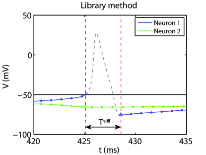
Figure 6: Illustration of the library method for two HH neurons unidirectionally connected from neuron 1 to neuron 2. After neuron 1 fires a spike, we compute and record the values $I^{\textrm{th}},m^{\textrm{th}},h^{\textrm{th}},n^{\textrm{th}}$, then we stop evolving its $V,m,h,n$ for the following $T^{\textrm{stiff}}$ ms and restart with the values $V^{\textrm{re}},m^{\textrm{re}},h^{\textrm{re}},n^{\textrm{re}}$ interpolated from the library indicated by the triangle. The dots indicate the time nodes where we use the standard RK4 scheme. The green square indicates an update time node due to the synaptic spike from neuron 1.

We now illustrate how to use the library. Once a neuron’s membrane potential reaches the threshold, we first record the values $I^{\textrm{th}},m^{\textrm{th}},h^{\textrm{th}},n^{\textrm{th}}$, then stop evolving this neuron’s equations of $V,m,h,n$ for the following $T^{\textrm{stiff}}$ ms and restart with values $V^{\textrm{re}},m^{\textrm{re}},h^{\textrm{re}},n^{\textrm{re}}$ linearly interpolated from the pre-computed high resolution data library as shown in Fig. 6. For the easy of writing, suppose $I^{\textrm{th}}$ falls between two data points $I_{0}^{\textrm{th}}$ and $I_{1}^{\textrm{th}}$ in the library. Simultaneously we can find the data points $m_{0}^{\textrm{th}}$ and $m_{1}^{\textrm{th}}$, $h_{0}^{\textrm{th}}$ and $h_{1}^{\textrm{th}}$, $n_{0}^{\textrm{th}}$ and $n_{1}^{\textrm{th}}$, respectively. So we need 16 suites of values in the library to perform a linear interpolation

$$z^{\textrm{re}}=\sum_{i,j,k,l=0,1}z^{\textrm{re}}(I_{i}^{\textrm{th}},m_{j}^{\textrm{th}},h_{k}^{\textrm{th}},n_{l}^{\textrm{th}})\frac{I^{\textrm{th}}-I_{1-i}^{\textrm{th}}}{I_{i}^{\textrm{th}}-I_{1-i}^{\textrm{th}}}\frac{m^{\textrm{th}}-m_{1-j}^{\textrm{th}}}{m_{j}^{\textrm{th}}-m_{1-j}^{\textrm{th}}}\frac{h^{\textrm{th}}-h_{1-k}^{\textrm{th}}}{h_{k}^{\textrm{th}}-h_{1-k}^{\textrm{th}}}\frac{n^{\textrm{th}}-n_{1-l}^{\textrm{th}}}{n_{l}^{\textrm{th}}-n_{1-l}^{\textrm{th}}}$$ (25)

for $z=V,m,h,n$. We note that the parameters $G$ and $H$ have analytic solutions, so they can be evolved as usual during the stiff period. After obtaining the high resolution library, we can use a large time step to evolve the HH neuron network with standard RK4 method. Detailed library algorithm is the same as the Algorithm 1 except that the step 13 should be replaced by the following algorithm.

Find the minimum of $\{t_{\text{spike}}^{(i)}\}$, say $t_{\text{spike}}^{(i_{1})}$. Evolve neuron $i_{1}$ to $t_{\text{spike}}^{(i_{1})}$, and generate a spike at this moment.

Record the values $I^{\textbf{th}},m^{\textbf{th}},h^{\textbf{th}},n^{\textbf{th}}$, then perform a linear interpolation from the library to get $V^{\textbf{re}},m^{\textbf{re}},h^{\textbf{re}},n^{\textbf{re}}$. Meanwhile, we stop evolving $V,m,h,n$ of neuron $i_{1}$ for the next $T^{\textbf{stiff}}$ ms, but we still evolve the conductance parameters $G,H$ as usual.

Update its postsynaptic neurons to $t_{\text{spike}}^{(i_{1})}$. Preliminarily evolve the affected neurons from $t_{\text{spike}}^{(i_{1})}$ to $t_{0}+\Delta t$ to update their spike times $\{t_{\text{spike}}\}$.

Algorithm 4 Library algorithm

6.3 Error of library method

There are three kinds of error in the library method: the error from the time step $\Delta t$, the error from the way of interpolation to use the library and the error from the assumption that we keep $I^{\textrm{input}}$ as constant throughout the stiff period $T^{\textrm{stiff}}$. The first one is simply $O(\Delta t^{4})$ since the library method is based on the RK4 scheme. The other two kinds of error come from the call of library. For simplicity, we consider the error of voltage for one single neuron to illustrate

$$\Delta V=|V_{\textrm{library}}-V_{\textrm{regular}}|$$ (26)

where $|\cdot|$ takes the absolute value, the subscript “regular” indicates the high precision solution computed by the RK4 method for a sufficiently small time step $\Delta t=2^{-16}$ ms and “library” indicates the solution from the library method.

The error from the way of interpolation can be well described by the error of the reset value $\Delta V^{\textrm{re}}$. We use a constant input $I^{\textrm{input}}$ to drive the HH neuron to exclude the influence of the assumption of constant input. Denote the sample intervals $\Delta I,\Delta m,\Delta h,\Delta n$ for $I^{\textrm{th}},m^{\textrm{th}},h^{\textrm{th}},n^{\textrm{th}}$, respectively. A linear interpolation yields an error of $\Delta V^{\textrm{re}}=O(\Delta I^{2}+\Delta m^{2}+\Delta h^{2}+\Delta n^{2})$. In our simulation, we take $\Delta I=2.5$ $\mu\textrm{A$\cdot$cm}^{-2}$, $\Delta m=\Delta h=\Delta n=0.02$ to build the library. If we use sample intervals $c\Delta I,c\Delta m,c\Delta h,c\Delta n$, then it is straight forward that $\Delta V^{\textrm{re}}=O(c^{2})$ as shown in Fig. 7(a) (Same results hold for $m,h,n$). In the same way, a cubic interpolation yields $\Delta V^{\textrm{re}}=O(c^{4})$ as shown in Fig. 7(b). Thus the cubic interpolation can indeed improve the accuracy when the network is driven by a constant input as shown in Fig. 7(c).

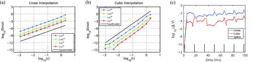
Figure 7: (a, b): The error of the reset values for a single HH neuron driven by constant input. (a) A linear interpolation and (b) a cubic interpolation to use the library. (c) The error of $\Delta V$ for a single HH neuron driven by constant input with a linear (blue) and cubic (red) interpolation to use the library. The short black lines indicate a spike. Time step is $\Delta t=2^{-16}$ ms for (a-c).

We now consider the error due to the assumption of constant input. Driven a single HH neuron by Poisson input, we compare the error of $\Delta V$ with different time steps and ways of interpolation to use the library as shown in Fig. 8. We find that once the neuron fires a spike and calls the library, the reset error $\Delta V^{\textrm{re}}$ (the dotted line in Fig. 8) is significantly greatly than the error of $\Delta V$ from the time step and way of interpolation. Therefore, the biggest error is from the assumption of constant input which cannot be reduced. Hence, we build a relatively coarse library and choose the linear interpolation to use the library in the Letter. Besides, we also find that the error of $\Delta V$ will not accumulate linearly with call number. As shown in Fig. 8, when the neuron fires, the error of $\Delta V$ will first raise to the level of $\Delta V^{\textrm{re}}$ and then quickly decay until the next spike time.

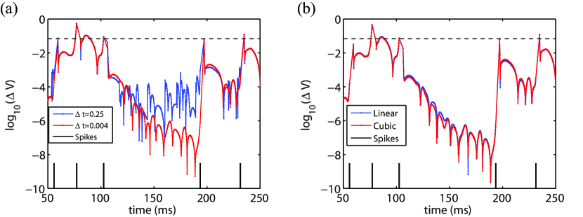
Figure 8: (a) The error of $\Delta V$ for one single neuron driven by Poisson input with a linear interpolation to use the library. Time steps are $\Delta t=0.25$ ms (blue) and $\Delta t=0.004$ ms (red). (b) The error of $\Delta V$ for one single neuron driven by Poisson input with a linear (blue) and cubic (red) interpolation to use the library, $\Delta t=0.004$ ms. The dotted line indicates the error of the reset value $\Delta V^{\textrm{re}}$ and the short black lines indicate a spike.

7 Numerical results

7.1 Hopf bifurcation of individual HH neuron

In this section, we show the performance of the given adaptive, ETD4RK and library methods with large time steps. We first exam whether the given methods can capture the type II behavior of individual HH neuron. Driven by constant input, the neuron can fire regularly and periodically [17, 18] only when the input current greater than a critical value $I^{\textrm{input}}\approx 6.2$ $\mu\textrm{A$\cdot$cm}^{-2}$. The HH model has a sudden jump around this critical value from zero firing rate to regular nonzero firing rate because of a subcritical Hopf bifurcation [18], as shown in Figure 9(a). Below the critical value, some spikes may appear before the neuron converges to stable zero firing rate state. The number of spikes during this transient period depends on how close the constant input is to the critical value, as shown in Figure 9(b). We point out that all the adaptive, ETD4RK and library method with time steps 8 time greater than that of the regular method can capture the type II behavior. Especially, the original library method in Ref. [14] fails to capture the spikes in the transient period since they use stable information of $V,m,h,$ and $n$ to build the library. Our library method uses the more intuitive suit of $V,m,h$ and $n$ to build the library which already covers both the possible stable and transient cases and is thus more precise.

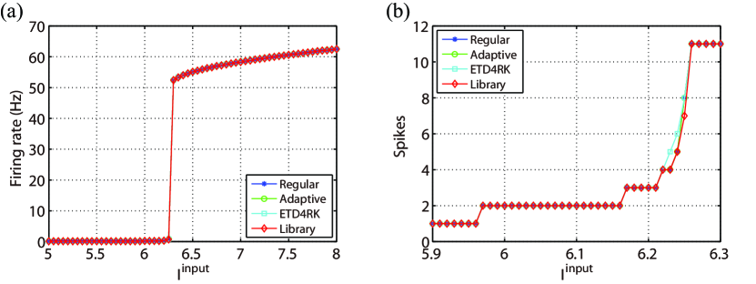
Figure 9: (a) The firing rate as a function of constant input $I^{\textrm{input}}$ ($\mu\textrm{A$\cdot$cm}^{-2}$). (b) The number of spikes during the transient period with initial voltage $V=-65$ mV. The blue stars, green circles, cyan squares and red diamonds in (a) and (b) indicate the results using regular method with $\Delta t=1/32$ ms, adaptive, ETD4RK and library method with $\Delta t=1/4$ ms, respectively.

7.2 Lyapunov exponent

For the performance of a network, we mainly consider a homogeneously and randomly connected network of 100 excitatory neurons with connection probability 10%, feedforward Poisson input $\nu=100$ Hz and $f=0.1$ $\textrm{mS$\cdot$cm}^{-2}$. Then the coupling strength $S$ is the only remaining variable. Other types of HH network and other dynamic regimes can be easily extended and similar results can be obtained.

We first study the chaotic dynamical property of the HH system by computing the largest Lyapunov exponent which is one of the most important tools to characterize chaotic dynamics [19]. The spectrum of Lyapunov exponents can measure the average rate of divergence or convergence of the reference and the initially perturbed orbits [20, 21, 22]. If the largest Lyapunov exponent is positive, then the reference and perturbed orbits will exponentially diverge and the dynamics is chaotic, otherwise, they will exponentially converge and the dynamics is non-chaotic.

When calculating the largest Lyapunov exponent, we use $\mathbf{X}=[X_{1},X_{2},...,X_{N}]$ to represent all the variables of the neurons in the HH model. Denote the reference and perturbed trajectories by $\mathbf{X}(t)$ and $\mathbf{\tilde{X}}(t)$, respectively. The largest Lyapunov exponent can be computed by

$$\lim_{t\rightarrow\infty}\lim_{\epsilon\rightarrow 0}\frac{1}{t}\ln\frac{||\mathbf{\tilde{X}}(t)-\mathbf{X}(t)||}{||\epsilon||}$$ (27)

where $\epsilon$ is the initial separation. However we cannot use Eq. (27) to compute directly, because for a chaotic system the separation $||\mathbf{\tilde{X}}(t)-\mathbf{X}(t)||$ is unbounded as $t\rightarrow\infty$ and a numerical ill-condition will happen. The standard algorithm to compute the largest Lyapunov exponent can be found in Ref. [22, 23, 24]. The regular, ETD4RK and adaptive methods can use these algorithms directly. However, for the library method, the information of $V,m,h,n$ are blank during the stiff period and these algorithms do not work. We use the extended algorithm introduced in Ref. [25] to solve this problem.

As shown in Fig. 10(a), we compute the largest Lyapunov exponent as a function of coupling strength $S$ from 0 to 0.1 $\textrm{mS$\cdot$cm}^{-2}$ by the regular, adaptive, ETD4RK and library methods, respectively. The total run time $T$ is 60 seconds which is sufficiently long to have convergent results. The adaptive, ETD4RK and library methods with large time steps ($\Delta t=1/4$ ms) can all obtain accurate largest Lyapunov exponent compared with the regular method. It shows three typical dynamical regimes that the system is chaotic in $0.037\lesssim S\lesssim 0.068$ $\textrm{mS$\cdot$cm}^{-2}$ with positive largest Lyapunov exponent and the system is non-chaotic in $0\lesssim S\lesssim 0.037$ and $0.068\lesssim S\lesssim 0.1$ $\textrm{mS$\cdot$cm}^{-2}$.

As shown in Fig. 10(b), we compute the mean firing rate, denoted by $R$, obtained by these methods to further demonstrate how accurate the adaptive, ETD4RK and library methods are. We give the relative error in the mean firing rate, which is defined as

$$E_{\textrm{R}}=|R_{*}-R_{\textrm{regular}}|/R_{\textrm{regular}}$$ (28)

where $*=\textrm{adaptive, ETD4RK, library}$. As shown in Fig. 10(c), all the given three methods can achieve at least 2 digits of accuracy using large time steps ($\Delta t=1/4$ ms). Note that the relative error may be zero in some cases and we set the logarithmic relative error -8 in Fig. 10(c), if it happens. Therefore, the adaptive method has a bit advantage over the ETD4RK and library methods for the mean firing rate.

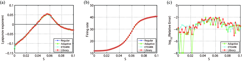
Figure 10: (a) The largest Lyapunov exponent of the HH network versus the coupling strength $S$. (b) Mean firing rate versus the coupling strength $S$. (c) The relative error in the mean firing rate (the Y-coordinate value -8 indicates there is no error). The blue, green, cyan and red curves represent the regular, adaptive, ETD4RK and library methods, respectively. The time steps are used as $\Delta t=1/32$ ms in the regular method and $\Delta t=1/4$ ms in the adaptive, ETD4RK and library methods. The total run time is 60 seconds to obtain convergent results.

From the calculation of the largest Lyapunov exponent, we have known that there are three typical dynamical regimes in the HH model. As shown in Fig. 11, these three regimes are asynchronous regime in $0\lesssim S\lesssim 0.037$ $\textrm{mS$\cdot$cm}^{-2}$, chaotic regime in $0.037\lesssim S\lesssim 0.068$ $\textrm{mS$\cdot$cm}^{-2}$ and synchronous regime in $0.068\lesssim S\lesssim 0.1$ $\textrm{mS$\cdot$cm}^{-2}$. So we choose three coupling strength $S=0.02,0.05$ and $0.08$ $\textrm{mS$\cdot$cm}^{-2}$ to represent these three typical dynamical regimes respectively in the following numerical tests.

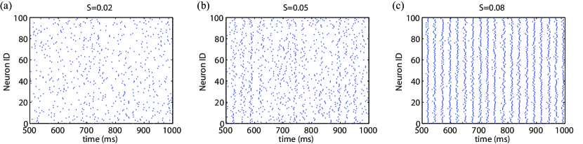
Figure 11: Raster plots of firing events in three typical dynamical regimes with coupling strength (a) $S=0.02$ $\textrm{mS$\cdot$cm}^{-2}$, (b) $S=0.05$ $\textrm{mS$\cdot$cm}^{-2}$, (c) $S=0.08$ $\textrm{mS$\cdot$cm}^{-2}$. Since all the given methods have almost the same raster, we only show the result obtained by the regular method.

7.3 Convergence tests

We now verify whether the algorithms given above have a fourth-order accuracy by performing convergence tests. For each method, we use a sufficiently small time step $\Delta t=2^{-16}$ ms ($\Delta t_{S}=2^{-16}$ ms for adaptive method) to evolve the HH model to obtain a high precision solution $\mathbf{X}^{\textrm{high}}$ at time $t=2000$ ms. To perform a convergence test, we also compute the solution $\mathbf{X}^{(\Delta t)}$ using time steps $\Delta t=2^{-4},2^{-5},...,2^{-10}$ ms. The numerical error is measured in the $L^{2}$ -norm

$$E=||\mathbf{X}^{(\Delta t)}-\mathbf{X}^{\textrm{high}}||$$ (29)

As shown in Fig. 12(a), the regular method can achieve a fourth-order accuracy for the non-chaotic regimes $S=0.02$ and $0.08$ $\textrm{mS$\cdot$cm}^{-2}$. For the chaotic one $S=0.05$ $\textrm{mS$\cdot$cm}^{-2}$, we can never achieve convergence of the numerical solution. The adaptive, ETD4RK and library methods have similar convergence phenomena as shown in Fig. 12.

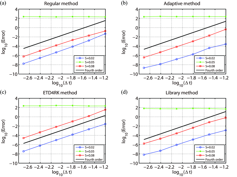
Figure 12: Convergence tests of (a) regular method, (b) adaptive method, (c) ETD4RK method and (d) library method. The convergence tests are performed by evolving the HH model for a total run time of $T=2000$ ms. We show the results for the coupling strength $S=0.02\textrm{ (blue)},0.05\textrm{ (green)}$ and $0.08$ (red) $\textrm{mS$\cdot$cm}^{-2}$, respectively.

7.4 Computational efficiency

In this section, we compare the efficiency among the adaptive, ETD4RK and library methods. A straight forward way is to compare the time cost of each method with a same total run time $T$. We notice that all the methods are based on the standard RK4 scheme, so we can compare the call number of the standard RK4 scheme that each method costs to give an analytical comparison of efficiency. For the ETD4RK method, the computational cost of one standard ETD4RK scheme is a bit more than that of the strand RK4 scheme. Here we omit the difference and no longer distinguish them for simplicity.

We start by exploring the call number of standard RK4 scheme for one neuron for one single time step with the regular method, which is presented in Theorem 1.

Theorem 1.

Suppose the presynaptic spike train to a neuron can be modeled by a Poisson train with rate $\lambda$, then the call number of standard RK4 scheme for the neuron for one time step from $t_{0}$ to $t_{0}+\Delta t$ in the regular method is $1+\nu\Delta t+(2\Delta t+\nu\Delta t^{2})\lambda$ on average.

• During the initial preliminary evolving from $t_{0}$ to $t_{0}+\Delta t$, it requires a call number of $1+\nu\Delta t$ on average. Suppose there are $n$ spikes fired by the presynaptic neurons during $[t_{0},t_{0}+\Delta t]$ which happens with probability $\frac{(\lambda\Delta t)^{n}}{n!}e^{-\lambda\Delta t}$. Denote the spike times by $t_{1},t_{2},...,t_{n}$, where $t_{0}<t_{1}<t_{2}<...,t_{n}<t_{0}+\Delta t$. For the $k$-th spike, as stated in Algorithm 1, it should first update from time $t_{k-1}$ to $t_{k}$ and then preliminarily evolve from $t_{k}$ to $t_{0}+\Delta t$ to update its next spike time $t_{\text{spike}}$. So the call number due to the $k$-th spike is $2+\nu(t_{0}+\Delta t-t_{k-1})=2+\nu\Delta t(1-\frac{t_{k-1}-t_{0}}{\Delta t})$ on average. Then the total average extra call number due to presynaptic neurons is

  $$2n+\nu\Delta t+\nu\Delta t\sum_{k=1}^{n-1}(1-\frac{t_{k}-t_{0}}{\Delta t})$$ (30)

  Under the condition of $n$ spikes, the distribution of $\frac{t_{1}-t_{0}}{\Delta t},\frac{t_{2}-t_{0}}{\Delta t},...,\frac{t_{n}-t_{0}}{\Delta t}$ is the same as the order statistics of $n$ independent and uniform distribution $U(0,1)$. Therefore, we have

  $$\mathbb{E}\left(\nu\Delta t\sum_{k=1}^{n-1}(1-\frac{t_{k}-t_{0}}{\Delta t})\Big{|}n\textrm{ spikes}\right) =\nu\Delta t\sum_{k=1}^{n-1}\intop_{0}^{1}\frac{n!}{(k-1)!(n-k)!}x^{k-1}(1-x)^{n-k+1}dx$$ (31)

  $$=\nu\Delta t\frac{(n-1)(n+2)}{2(n+1)}$$

  where $\mathbb{E}$ takes the expectation. Hence the expected extra call number due to these spikes is

  $$\mathbb{E}\left(2n+\nu\Delta t+\nu\Delta t\frac{(n-1)(n+2)}{2(n+1)}\right) =\sum_{n=1}^{\infty}\left(2n+\nu\Delta t+\nu\Delta t\frac{(n-1)(n+2)}{2(n+1)}\right)\frac{(\lambda\Delta t)^{n}}{n!}e^{-\lambda\Delta t}$$ (32)

  $$=(2\lambda+\nu)\Delta t+\frac{\lambda\nu}{2}\Delta t^{2}+\frac{\nu}{\;\lambda}(e^{-\lambda\Delta t}-1)$$

  $$=2\lambda\Delta t+\lambda\nu\Delta t^{2}+o(\Delta t^{2})$$

  Therefore, the expected call number for one neuron for one time step in regular method is $1+\nu\Delta t+(2\Delta t+\nu\Delta t^{2})\lambda$. ∎

We suppose the spike events of presynaptic neurons are a Poisson train since they can be asymptotically approach a Poisson process [26, 27] when the spike timing are irregular. Once a neuron fires a spike, it should also update to this spike time and then preliminarily evolve to update its next spike time $t_{\textrm{spike}}$, so the Poisson spike train it goes through has rate $(1+p_{c}N)R$, where the 1 corresponds to the spikes it fires and $p_{c}$ is the connection probability. Therefore, the average call number per neuron for the regular method is

$$\left\langle\mathcal{N}_{\textrm{regular}}\right\rangle=\frac{T}{\Delta t}[1+\nu\Delta t+(2\Delta t+\nu\Delta t^{2})(1+p_{c}N)R]$$ (33)

Note that regular and ETD4RK method have the same formula of call number.

For the adaptive method, it is based on the regular method, so it also has the required call number in Eq. (33) . Besides, we should add the extra call number due to the smaller time step $\Delta t_{S}$ during the stiff period. For the spike the neuron fires, it requires extra call number of $TRT^{\textrm{stiff}}/\Delta t_{S}$. For the presynaptic spikes, similar to Theorem 1, the extra call number is $p_{c}NTRp\Delta t/\Delta t_{S}$, where $p$ is the probability that the neuron is in the stiff period when its presynaptic neurons fire. Therefore, we have

$$\left\langle\mathcal{N}_{\textrm{adaptive}}\right\rangle \approx\frac{T}{\Delta t}[1+\nu\Delta t+(2\Delta t+\nu\Delta t^{2})(1+p_{c}N)R]+TR\frac{T^{\textrm{stiff}}}{\Delta t_{S}}+p_{c}NTRp\frac{\Delta t}{\Delta t_{S}}$$ (34)

For the library method, once a neuron fires a spike, we do not evolve its $V,m,h,n$ for the next $T^{\textrm{stiff}}$ ms, $\mathit{i.e.}$, no call of the standard RK4 scheme. With a little amendment of Eq. (33), we have

$$\left\langle\mathcal{N}_{\textrm{library}}\right\rangle\approx(1-T^{\textrm{stiff}}R)\frac{T}{\Delta t}(1+\nu\Delta t)+\frac{T}{\Delta t}(2\Delta t+\nu\Delta t^{2})(R+p_{c}NR(1-p))$$ (35)

where $T^{\textrm{stiff}}R$ is the probability that a neuron stays in the stiff period.

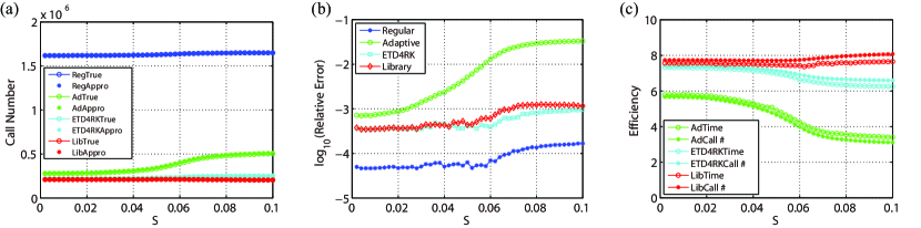
Figure 13: (a) The call number of standard RK4 scheme per neuron for the regular, adaptive, ETD4RK and library methods. The circles represent the call number from numerical tests while the stars represent the approximations from Eqs. (33)-(35). (b) The relative error in the call number between the approximation and numerical tests for the regular, adaptive, ETD4RK and library methods. (c) The efficiency measured by the time cost and call number versus the coupling strength $S$ for the adaptive, ETD4RK and library methods. Time steps and colors are the same as the one in Fig. 10. Total run time is 50 seconds.

As shown in Fig. 13, we count the call numbers from the numerical tests and approximations in Eqs. (33-35) for the regular, adaptive, ETD4RK and library methods, respectively. These equations are indeed close approximations of the call number achieving at least 1 digit of accuracy. We should point out that the information of $R$ and $p$ in the approximations are obtained from the numerical tests since they are hard to estimate directly.

Fig. 13(c) gives the efficiency of the adaptive, ETD4RK and library methods by comparing the time cost and call number with that of the regular method. These two kinds of efficiency are quite consistent except a bit difference in the ETD4RK and library methods. For the ETD4RK method, this is because we use the standard ETD4RK scheme during the stiff period which costs a bit more time than the standard RK4 scheme. So the efficiency measured by the call number is a bit overestimated. For the library method, this is because when a neuron fires a spike, we should call the library and evolve the parameters $G$ and $H$ during the stiff period which costs some time but is not included in the efficiency measured by the call number. When the mean firing rate is high, this extra consumed time is no longer negligible. Even so, these two kinds of efficiency still show good agreement for the ETD4RK and library methods. Therefore, we can use the efficiency measured by the call number to compare.

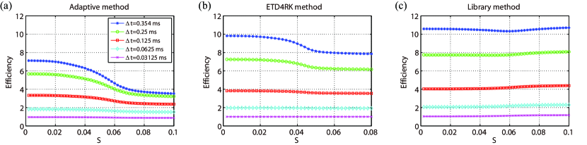
Figure 14: Efficiency measured by the expected call number for the adaptive, ETD4RK and library methods, respectively. The time steps are $\Delta t=0.354,0.25,0.125,0.0625,0.03125$ ms from top to bottom. Total run time is 50 seconds.

Fig. 14 shows the efficiency for the adaptive, ETD4RK and library methods with different time steps. When the mean firing rate is low ($\leq 20$ Hz), the adaptive method can achieve high efficiency with a maximum 7 times of speedup. However this high efficiency decreases rapidly with the coupling strength (mean firing rate), since the neurons will use the smaller time step much more often when the firing rate is high. The ETD4RK and library methods are not so sensitive to the firing rate and can achieve a global high efficiency. Especially, the library method can achieve a maximum 10 times of speedup for the maximum time step $\Delta t=0.354$ ms.

8 Conclusion

In conclusion, we have shown three methods to deal with the stiff part during the firing event in evolving the HH equations. All of them can use a large time step to save computational cost. The adaptive method is the easiest to use and can retain almost all the information of the original HH neurons like the spike shapes. However, it has limited efficiency and is more appropriate for the dynamical regimes with low firing rate. The ETD4RK method can obtain both precise trajectory of the variables and high efficiency. The library method achieves the highest efficiency, but it sacrifices the accuracy of spike shapes and is more suitable for high accurate statistical information of HH neuronal networks.

For the adaptive method, we should point out that the standard adaptive method like the Runge-Kutta-Fehlberg method is not suitable for the HH neuronal networks. When evolving a single neuron, the standard adaptive method requires an extra RK4 calculation to decide the adaptive time step. When the neuron fires, its equations become stiff and the chosen time step is very small $\sim 1/32$ ms as illustrated in Ref. [8]. So it is no better than our adaptive method for a single neuron. For networks, the standard adaptive method should evolve the entire network to choose the adaptive time step. For large-scaled networks, there are firing events almost everywhere, then the chosen adaptive time step is always quite small $1/32$ ms [8] and makes the method ineffective.

Our library method is based on the original work in Ref. [14]. The main difference is the way to build and use the library. In the original work, once the membrane potential reaches the threshold, we should record the input current $I^{\textrm{th}}$ and gating variables $m^{\textrm{th}},h^{\textrm{th}},n^{\textrm{th}}$. Driving a single neuron with constant input $I^{\textrm{th}}$, we will obtain a periodic trajectory of membrane potential after the transient period. Especially we intercept a stable section of the trajectory whose initial value is the threshold $V^{\text{th}}$ and data length is the stiff period. Given the section of membrane potential and initial values $m^{\textrm{th}},h^{\textrm{th}},n^{\textrm{th}}$, we can obtain the corresponding reset gating variables $m^{\textrm{re}},h^{\textrm{re}},n^{\textrm{re}}$, respectively. Denote the sample number of $I^{\textrm{th}},m^{\textrm{th}},h^{\textrm{th}},n^{\textrm{th}}$ by $N_{I},N_{m},N_{n},N_{h}$, then the size of library is $N_{I}(1+N_{m}+N_{n}+N_{h})$, $i.e.$, the input current $I^{\textrm{th}}$ is the most important. In our library method, the gating variables are as important as the input current. Given a suite of $I^{\textrm{th}},m^{\textrm{th}},h^{\textrm{th}},n^{\textrm{th}}$, we evolve the HH equations with constant input $I^{\textrm{th}}$ for $T^{\textrm{stiff}}$, then we can obtain the corresponding reset values $I^{\textrm{re}},m^{\textrm{re}},h^{\textrm{re}},n^{\textrm{re}}$ simultaneously. The advantage of our library method lies in two aspects: 1) It is much easier to build the library. 2) Our data library is much accurate since it can cover both the transient and the stable periodic information.

Finally, we emphasize that the spike-spike correction procedure [7] is necessary in the given methods to achieve an accuracy of fourth-order. However, it will greatly decrease the efficiency of the advanced ETD4RK and library methods for large-scaled networks. When there are many neurons that fire in one time step, each neuron will call the standard RK4 scheme a lot during the updating and preliminary evolving procedure. When the size of the network tends infinity, the given methods with large time step will even slower than the regular method with a small time step as illustrated in Eqs. (33), (34) and 35). We point out that this problem can be solved by reducing the accuracy from the fourth-order to a second-order. In each time step, we evolve each neuron without considering the feedforward and synaptic spikes and recalibrate their effects at the end of the time step. Then the spike-spike correction procedure is avoided while the methods still have an accuracy of second-order [13]. Besides, the call number per neuron is merely $T/\Delta t$ for regular and ETD4RK methods and $(1-T^{\textrm{stiff}}R)T/\Delta t$ for the library method. Therefore, the ETD4RK and library methods can stably achieve over 10 times of speedup with a large time step in any kinds of networks, $e.g.$, all-to-all connected networks, large-scaled networks and network of both excitatory and inhibitory neurons.

Appendix: Parameters and variables for the Hodgkin-Huxley equations

Definitions of $\alpha$ and $\beta$ are as follows [28]:

$\alpha_{m}(V)=(0.1V+4)/(1-\exp(-0.1V-4)),$

$\beta_{m}(V)=4\exp(-(V+65)/18),$

$\alpha_{h}(V)=0.07\exp(-(V+65)/20),$

$\beta_{h}(V)=1/(1+\exp(-3.5-0.1V)),$

$\alpha_{n}(V)=(0.01V+0.55)/(1-\exp(-0.1V-5.5)),$

$\beta_{n}(V)=0.125\exp(-(V+65)/80)$.

Other model parameters are set as $C=1\mu\textrm{F$\cdot$cm}^{-2}$, $V_{Na}=50$ mV, $V_{K}=-77$ mV, $V_{L}=-54.387$ mV, $G_{Na}=120\textrm{ mS$\cdot$cm}^{-2}$, $G_{K}=36\textrm{ mS$\cdot$cm}^{-2}$, $G_{L}=0.3\textrm{ mS$\cdot$cm}^{-2}$, $V_{G}=0$ mV, $\sigma_{r}=0.5$ ms, and $\sigma_{d}=3.0$ ms [28].

References

- [1] Alan L Hodgkin and Andrew F Huxley. A quantitative description of membrane current and its application to conduction and excitation in nerve. The Journal of physiology, 117(4):500, 1952.
- [2] Brian Hassard. Bifurcation of periodic solutions of the hodgkin-huxley model for the squid giant axon. Journal of Theoretical Biology, 71(3):401–420, 1978.
- [3] Peter Dayan and LF Abbott. Theoretical neuroscience: computational and mathematical modeling of neural systems. Journal of Cognitive Neuroscience, 15(1):154–155, 2003.
- [4] David C Somers, Sacha B Nelson, and Mriganka Sur. An emergent model of orientation selectivity in cat visual cortical simple cells. Journal of Neuroscience, 15(8):5448–5465, 1995.
- [5] David McLaughlin, Robert Shapley, Michael Shelley, and Dingeman J Wielaard. A neuronal network model of macaque primary visual cortex (v1): Orientation selectivity and dynamics in the input layer 4c. Proceedings of the National Academy of Sciences, 97(14):8087–8092, 2000.
- [6] David Cai, Aaditya V Rangan, and David W McLaughlin. Architectural and synaptic mechanisms underlying coherent spontaneous activity in v1. Proceedings of the National Academy of Sciences of the United States of America, 102(16):5868–5873, 2005.
- [7] Aaditya V Rangan and David Cai. Fast numerical methods for simulating large-scale integrate-and-fire neuronal networks. Journal of Computational Neuroscience, 22(1):81–100, 2007.
- [8] Christoph Borgers and Alexander R Nectow. Exponential time differencing for hodgkin–huxley-like odes. SIAM Journal on Scientific Computing, 35(3):B623–B643, 2013.
- [9] Peter G Petropoulos. Analysis of exponential time-differencing for fdtd in lossy dielectrics. IEEE transactions on antennas and propagation, 45(6):1054–1057, 1997.
- [10] Steven M Cox and Paul C Matthews. Exponential time differencing for stiff systems. Journal of Computational Physics, 176(2):430–455, 2002.
- [11] Lili Ju, Xiao Li, Zhonghua Qiao, and Hui Zhang. Energy stability and error estimates of exponential time differencing schemes for the epitaxial growth model without slope selection. Mathematics of Computation, 87(312):1859–1885, 2018.
- [12] David Hansel, Germán Mato, Claude Meunier, and L Neltner. On numerical simulations of integrate-and-fire neural networks. Neural Computation, 10(2):467–483, 1998.
- [13] Michael J Shelley and Louis Tao. Efficient and accurate time-stepping schemes for integrate-and-fire neuronal networks. Journal of Computational Neuroscience, 11(2):111–119, 2001.
- [14] Yi Sun, Douglas Zhou, Aaditya V Rangan, and David Cai. Library-based numerical reduction of the hodgkin–huxley neuron for network simulation. Journal of computational neuroscience, 27(3):369–390, 2009.
- [15] Sen Song, Per Jesper Sjöström, Markus Reigl, Sacha Nelson, and Dmitri B Chklovskii. Highly nonrandom features of synaptic connectivity in local cortical circuits. PLoS biology, 3(3):e68, 2005.
- [16] Yuji Ikegaya, Takuya Sasaki, Daisuke Ishikawa, Naoko Honma, Kentaro Tao, Naoya Takahashi, Genki Minamisawa, Sakiko Ujita, and Norio Matsuki. Interpyramid spike transmission stabilizes the sparseness of recurrent network activity. Cerebral Cortex, 23(2):293–304, 2012.
- [17] Wulfram Gerstner and Werner M Kistler. Spiking neuron models: Single neurons, populations, plasticity. Cambridge university press, 2002.
- [18] Christof Koch and Idan Segev. Methods in neuronal modeling: from ions to networks. MIT press, 1998.
- [19] Valery Iustinovich Oseledec. A multiplicative ergodic theorem. lyapunov characteristic numbers for dynamical systems. Trans. Moscow Math. Soc, 19(2):197–231, 1968.
- [20] Edward Ott. Chaos in dynamical systems. Cambridge university press, 2002.
- [21] John Michael Tutill Thompson and H Bruce Stewart. Nonlinear dynamics and chaos. John Wiley & Sons, 2002.
- [22] Thomas S Parker and Leon Chua. Practical numerical algorithms for chaotic systems. Springer Science & Business Media, 2012.
- [23] Douglas Zhou, Yi Sun, Aaditya V Rangan, and David Cai. Spectrum of lyapunov exponents of non-smooth dynamical systems of integrate-and-fire type. Journal of computational neuroscience, 28(2):229–245, 2010.
- [24] Alan Wolf, Jack B Swift, Harry L Swinney, and John A Vastano. Determining lyapunov exponents from a time series. Physica D: Nonlinear Phenomena, 16(3):285–317, 1985.
- [25] Douglas Zhou, Aaditya V Rangan, Yi Sun, and David Cai. Network-induced chaos in integrate-and-fire neuronal ensembles. Physical Review E, 80(3):031918, 2009.
- [26] Peter AW Lewis. Stochastic point processes: statistical analysis, theory, and applications. 1972.
- [27] Erhan Cinlar and RA Agnew. On the superposition of point processes. Journal of the Royal Statistical Society. Series B (Methodological), pages 576–581, 1968.
- [28] Peter Dayan and Laurence F Abbott. Theoretical neuroscience, volume 806. Cambridge, MA: MIT Press, 2001.