A General 3D Non-Stationary Massive MIMO GBSM for 6G Communication Systems

Abstract

A general three-dimensional (3D) non-stationary massive multiple-input multiple-output (MIMO) geometry-based stochastic model (GBSM) for the sixth generation (6G) communication systems is proposed in the paper. The novelty of the model is that the model is designed to cover a variety of channel characteristics, including space-time-frequency (STF) non-stationarity, spherical wavefront, spatial consistency, channel hardening, etc. Firstly, the introduction of the twin-cluster channel model is given in detail. Secondly, the key statistical properties such as space-time-frequency correlation function (STFCF), space cross-correlation function (CCF), temporal autocorrelation function (ACF), frequency correlation function (FCF), and performance indicators, e.g., singular value spread (SVS), and channel capacity are derived. Finally, the simulation results are given and consistent with some measurements in relevant literatures, which validate that the proposed channel model has a certain value as a reference to model massive MIMO channel characteristics.

I Introduction

Compared with the fifth generation (5G) communication systems, the 6G communication systems have attracted more and more attention because of almost a thousand times transmission rate and capacity[1], [2]. Massive MIMO technology is an efficient way to increase capacity and spectral efficiency for 6G communication systems, which refers to that the base station (BS) is equipped with a large number of antennas up to one hundred or even thousands of antennas. Besides, with more and more antennas exploited at BS side, the channel among different users become approximatively orthogonal, which is called channel hardening phenomenon (or favorable propagation conditions)[3], [4]. Therefore, the interference among the users can be removed, which makes the 6G communication systems inherently robust.

There are mainly three new characteristics for massive MIMO channel: spherical wavefront, spatial non-stationarity, and channel hardening phenomenon. Spherical wavefront refers to that the distance between the transmitter (Tx) and receiver (Rx) or cluster is less than the Rayleigh distance $2L^{2}/\lambda$, where $L$ represents the antenna array size, $\lambda$ denotes the wavelength. Channel measurements showed that the angle of departure (AoD) along the antenna array gradually shifts[5] and line-of-sight (LOS) path azimuth angle shifts along the array[6], which demonstrated the spherical wavefront. Birth-death process along the array brings spatial non-stationarity. The clusters appear and disappear along the array randomly, which was verified by the fact that received power of LOS path varies along the array [6]. In [7], theoretical analysis showed that the correlation matrix at user side becomes a diagonal matrix under favorable propagation conditions and channel hardening phenomenon is obvious. The above characteristics bring new requirements for massive MIMO channel modeling.

A general massive MIMO channel model for 6G communication systems should be at least suitable for millimeter wave communications, vehicle-to-vehicle (V2V) communications, 3D communication environments, and high-speed train (HST) communications. In [8], a two-dimensional (2D) parabolic wavefront model was proposed, and a 3D parabolic wavefront model was further developed [9]. However, the model only considered the movements of the Rx and clusters, so it was not applicable to V2V scenario. Similarly, a twin-cluster channel model in [10] did not consider the movement of the Tx. A general 3D non-stationary 5G channel model and a general 3D non-stationary channel model for 5G and beyond were given in [11] and [12], respectively. The two models only considered the cluster evolution in space domain and time domain, which was not suitable for millimeter wave communication systems needing to consider cluster evolution in frequency domain. References [13] and [14] demonstrated a multi-ring channel model and a multi-confocal ellipse channel model, respectively. Both of them were 2D channel models without considering elevation characteristic. Reference [15] proposed a 3D ellipsoid model, which did not consider the movement of the Tx and cluster. Reference [16] proposed a millimeter wave massive MIMO channel for HST communications without considering spatial consistency and V2V communications. The above mentioned channel models do not consider all the requirements for 6G massive MIMO channel modeling.

To the best of our knowledge, the general 3D massive MIMO GBSM considering STF cluster evolution, spherical wavefront, spatial consistency, and channel hardening for 6G communication systems is still missing in the literature. This paper presents a general 3D massive MIMO GBSM based on the model in [12] so as to fill the above research gaps. The contributions of the paper are summarized as follows. Firstly, the proposed channel model is suitable for millimeter wave communications, V2V communications, 3D communication environments, and HST communications by adjusting channel parameters. Secondly, the cluster evolution is further extended from space and time domain in [12] to STF domain. Thirdly, the large scale parameters (LSPs) and small scale parameters (SSPs) are generated according to the positions of Tx and Rx using the sum-of-sinusoids (SoS) method, which makes the model inherently spatially consistent. Finally, the STF non-stationarity, spatial consistency, and channel hardening characteristics are verified by simulation results.

The remaining paper is structured as follows. Section II describes the proposed general massive MIMO GBSM in detail. In Section III, statistical properties and performance indicators of the presented model are derived. Simulation results and analysis are given in Section IV. Finally, conclusions are drawn in Section V.

II A general Massive MIMO GBSM

As illustrated in Fig. 1, large uniform rectangular arrays (URAs) are adopted at the BS and mobile station (MS) sides in this model. Suppose that the BS is Tx and the MS is Rx. The URA at BS (MS) side is formed by uniform linear arrays (ULAs) in two dimensions. There are $M_{T}$ ($M_{R}$) antenna elements symboled as $A_{p}^{T}$ ($p=1,2,\cdots,M_{T}$) ( $A_{q}^{R}$ ($q=1,2,\cdots,M_{R}$)) and spaced at a distance $\delta_{T}$ ($\delta_{R}$) in one dimension. In another dimension, there are $N_{T}$ ($N_{R}$) antenna elements symboled as $A_{u}^{T}$ ($u=1,2,\cdots,N_{T}$) ($A_{v}^{R}$ ($v=1,2,\cdots,N_{R}$)) spaced at a distance $\delta_{T}$ ($\delta_{R}$). In the $M_{T}$ ($M_{R}$) antenna elements dimension, the angle of elevation is $\beta_{E}^{T}$ ($\beta_{E}^{R}$) and the angle of azimuth is $\beta_{A}^{T}$ ($\beta_{A}^{R}$). In order to calculate conveniently, we consider the $M_{T}$ ($M_{R}$) antenna elements as a ULA. All the ULAs in the $N_{T}$ ($N_{R}$) antenna elements dimension can be added to form the whole URA. Multi-bounce propagation is simplified as twin-cluster propagation. The path between the first bounce cluster $C_{n}^{A}$ and the last bounce cluster $C_{n}^{Z}$ is abstracted by a virtual link. The total number of paths from $A_{p}^{T}$ to $A_{q}^{R}$ at time $t$ is $N_{qp}(t)$. The number of scatterers in the $n$th path is $M_{n}(t)$. The Tx, Rx, and clusters can move with arbitrary velocities and trajectories. Furthermore, all the parameters are time-variant. For clarity, the remaining definitions of the parameters are shown in Table  I.

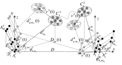
Figure 1: A general 3D massive MIMO GBSM for 6G communication systems.

TABLE I: Definition of Key Channel Model Parameters.

Parameters	Definition
$f_{c}$	Carrier frequency
$D$	Distance from $A_{1}^{T}$ to $A_{1}^{R}$ at initial time
$d_{m_{n}}^{T(R)}$	Distance from $A_{1}^{T(R)}$ to the $m$th scatterer in $C_{n}^{A(Z)}$ at initial time
$d_{p(q),m_{n}}^{T(R)}(t)$	Distance from $A_{p(q)}^{T(R)}$ to the $m$th sactterer in $C_{n}^{A(Z)}$ at time $t$
$d_{qp,m_{n}}(t)$	Distance from $A_{p}^{T}$ through the $m$th scatterer in $C_{n}^{A}$ and the $m$th scatterer in $C_{n}^{Z}$ to $A_{q}^{R}$ at time $t$
$\tau_{qp,m_{n}}(t)$	Delay from $A_{p}^{T}$ through the $m$th scatterer in $C_{n}^{A}$ and the $m$th scatterer in $C_{n}^{Z}$ to $A_{q}^{R}$ at time $t$
$v^{T}(t)$, $v^{R}(t)$, $v^{A_{n}}(t)$, $v^{Z_{n}}(t)$	Speeds of the Tx, Rx, cluster $C_{n}^{A}$, and cluster $C_{n}^{Z}$ at time $t$
$\alpha_{A}^{T}(t)$, $\alpha_{A}^{R}(t)$, $\alpha_{A}^{A_{n}}(t)$,$\alpha_{A}^{Z_{n}}(t)$	Azimuth angles of movements of the Tx, Rx, cluster $C_{n}^{A}$, and cluster $C_{n}^{Z}$ at time $t$
$\alpha_{E}^{T}(t)$, $\alpha_{E}^{R}(t)$, $\alpha_{E}^{A_{n}}(t)$,$\alpha_{E}^{Z_{n}}(t)$	Elevation angles of movements of the Tx, Rx, cluster $C_{n}^{A}$, and cluster $C_{n}^{Z}$ at time $t$
$\phi_{A,{LOS}}^{T}$, $\phi_{E,{LOS}}^{T}$	Azimuth angle of departure (AAoD) and elevation angle of departure (EAoD) from $A_{1}^{T}$ to $A_{1}^{R}$ at initial time
$\phi_{A,{LOS}}^{R}$, $\phi_{E,{LOS}}^{R}$	Azimuth angle of arrival (AAoA) and elevation angle of arrival (EAoA) from $A_{1}^{R}$ to $A_{1}^{T}$ at initial time
$\phi_{A,m_{n}}^{T(R)}$, $\phi_{E,m_{n}}^{T(R)}$	AAoD (AAoA) and EAoD (EAoA) from $A_{1}^{T(R)}$ to the $m$th scatterer in $C_{n}^{A(Z)}$ at initial time
$P_{qp,m_{n}}(t)$	Power of the ray from $A_{p}^{T}$ through the $m$th scatterer in $C_{n}^{A}$ and the $m$th scatterer in $C_{n}^{Z}$ to $A_{q}^{R}$ at time $t$

II-A Channel Impulse Response (CIR)

The complete channel matrix is comprised of large scale fading (LSF) part and small scale fading (SSF) part. The LSF consists of path loss ($PL$), shadowing ($SH$), blockage loss ($BL$), and gas absorption loss ($AL$). The theoretical channel matrix is presented as

$$\textbf{H}=\left[PL\cdot SH\cdot BL\cdot AL\right]^{1/2}\textbf{H}_{s}$$ (1)

where $\textbf{H}_{s}$ is the SSF matrix and can be further represented as

$$\textbf{H}_{s}=\left[h_{qp}(t,\tau)\right]_{M_{R}N_{R}\times M_{T}N_{T}}$$ (2)

where $h_{qp}(t,\tau)$ can be acquired by the summation of LOS component and non-line-of-sight (NLOS) components.

$$h_{qp}(t,\tau)=\sqrt{\frac{K_{RF}(t)}{K_{RF}(t)+1}}h_{qp}^{L}(t,\tau)+\sqrt{\frac{1}{K_{RF}(t)+1}}h_{qp}^{N}(t,\tau)$$ (3)

where $K_{RF}(t)$ is Rician factor, $h_{qp}^{L}(t,\tau)$ is LOS component and $h_{qp}^{N}(t,\tau)$ NLOS components. LOS component can be represented as

$$\begin{split}&h_{qp}^{L}(t,\tau)=\left[\begin{matrix}F_{q,V_{p}}(\phi_{E,{LOS}}^{R}(t),\phi_{A,{LOS}}^{R}(t))\\ F_{q,H_{p}}(\phi_{E,{LOS}}^{R}(t),\phi_{A,{LOS}}^{R}(t))\end{matrix}\right]^{T}\\ &\cdot\left[\begin{matrix}e^{j\theta_{LOS}^{V_{p}V_{p}}}&0\\ 0&-e^{j\theta_{LOS}^{H_{p}H_{p}}}\end{matrix}\right]\left[\begin{matrix}F_{p,V_{p}}(\phi_{E,{LOS}}^{T}(t),\phi_{A,{LOS}}^{T}(t))\\ F_{p,H_{p}}(\phi_{E,{LOS}}^{T}(t),\phi_{A,{LOS}}^{T}(t))\end{matrix}\right]\\ &\cdot e^{j2\pi f_{c}\tau_{qp}^{LOS}(t)}\delta(\tau-\tau_{qp}^{LOS}(t)).\end{split}$$ (4)

NLOS components can be represented as

$$\begin{split}&h_{qp}^{N}(t,\tau)=\sum_{n=1}^{N_{qp}(t)}\sum_{m=1}^{M_{n}(t)}\left[\begin{matrix}F_{q,V_{p}}(\phi_{E,m_{n}}^{R}(t),\phi_{A,m_{n}}^{R}(t))\\ F_{q,H_{p}}(\phi_{E,m_{n}}^{R}(t),\phi_{A,m_{n}}^{R}(t))\end{matrix}\right]^{T}\\ &\cdot\left[\begin{matrix}e^{j\theta_{m_{n}}^{V_{p}V_{p}}}&\sqrt{\kappa_{m_{n}}^{-1}(t)}e^{j\theta_{m_{n}}^{V_{p}H_{p}}}\\ \sqrt{\kappa_{m_{n}}^{-1}(t)}e^{j\theta_{m_{n}}^{H_{p}V_{p}}}&e^{j\theta_{m_{n}}^{H_{p}H_{p}}}\end{matrix}\right]\\ &\cdot\left[\begin{matrix}F_{p,V_{p}}(\phi_{E,m_{n}}^{T}(t),\phi_{A,m_{n}}^{T}(t))\\ F_{p,H_{p}}(\phi_{E,m_{n}}^{T}(t),\phi_{A,m_{n}}^{T}(t))\end{matrix}\right]\sqrt{P_{qp,m_{n}}(t)}e^{j2\pi f_{c}\tau_{qp,m_{n}}(t)}\\ &\cdot\delta(\tau-\tau_{qp,m_{n}}(t))\end{split}$$ (5)

where $(\cdot)^{T}$ denotes the transpose operation. $F_{p(q),V_{p}}^{T(R)}(\cdot)$ and $F_{p(q),H_{p}}^{T(R)}(\cdot)$ represent the vertical polarization and horizontal polarization at Tx (Rx) side, respectively. $\kappa_{m_{n}}$ denotes the cross polarization ratio.

II-B Channel Transfer Function (CTF)

Take the Fourier transform of the CIR, we will get the CTF as

$$H_{qp}(t,f)= \sqrt{\frac{K_{RF}(t)}{K_{RF}(t)+1}}H_{qp}^{L}(t,f)$$

$$+\sqrt{\frac{1}{K_{RF}(t)+1}}H_{qp}^{N}(t,f).$$ (6)

where $H_{qp}^{L}(t,f)$ is LOS component and $H_{qp}^{N}(t,f)$ NLOS components.

II-C STF Cluster Evolution

The proposed channel has the characteristic of STF non-stationarity. Clusters may appear and disappear in STF domain. The space-time evolution is modeled jointly. For initial moment $t_{i}$ and antenna element $A_{p}^{T}$ ($A_{q}^{R}$), the cluster is represented as $C_{p}^{T}(t_{i})$ ($C_{q}^{R}(t_{i})$). At the next moment $t_{i}+\triangle t$, the cluster evolves into $C_{p+1}^{T}(t_{i}+\triangle t)$ ($C_{q+1}^{R}(t_{i}+\triangle t)$). The space-time evolution process can be modeled as

$$\begin{matrix}\,\,\,C_{p}^{T}(t_{i})\xrightarrow{E}C_{p+1}^{T}(t_{i}+\triangle t)&(p=1,2,\cdots,M_{T}-1)\end{matrix}$$ (7)

$$\begin{matrix}\,\,\,C_{q}^{R}(t_{i})\xrightarrow{E}C_{q+1}^{R}(t_{i}+\triangle t)&(q=1,2,\cdots,M_{R}-1).\end{matrix}$$ (8)

By defining $\lambda_{G}$ and $\lambda_{R}$ as the generation rate and recombination rate of the cluster, the survival probabilities of the clusters at Tx and Rx sides can be represented as

$$\begin{split}\begin{matrix}\indent P_{\text{survival}}^{T}(\triangle t,\delta_{p})=e^{-\lambda_{R}\left[(\epsilon_{1}^{T})^{2}+(\epsilon_{2}^{T})^{2}+2\epsilon_{1}^{T}\epsilon_{2}^{T}\text{cos}(\alpha_{A}^{T}-\beta_{A}^{T})\right]^{1/2}}\end{matrix}\end{split}$$ (9)

$$\begin{split}\begin{matrix}\indent P_{\text{survival}}^{R}(\triangle t,\delta_{q})=e^{-\lambda_{R}\left[(\epsilon_{1}^{R})^{2}+(\epsilon_{2}^{R})^{2}+2\epsilon_{1}^{R}\epsilon_{2}^{R}\text{cos}(\alpha_{A}^{R}-\beta_{A}^{R})\right]^{1/2}}\end{matrix}\end{split}$$ (10)

where $\epsilon_{1}^{T}=\frac{\delta_{p}cos\beta_{E}^{T}}{D_{c}^{A}},\delta_{p}=(p-1)\delta_{T},$ ($\epsilon_{1}^{R}=\frac{\delta_{q}cos\beta_{E}^{R}}{D_{c}^{A}},\delta_{q}=(q-1)\delta_{R}$), and $\epsilon_{2}^{T}=\frac{v_{T}\triangle t}{D_{c}^{S}}$ ($\epsilon_{2}^{R}=\frac{v_{R}\triangle t}{D_{c}^{S}}$) represent the distance differences caused by array evolution and time evolution, respectively. $D_{c}^{A}$ and $D_{c}^{S}$ are scenario-dependent coefficients in space domain and time domain, respectively. Combined with frequency evolution, the total survival probability is represented as

$$\begin{split}P_{\text{survival}}(\triangle t,\delta_{p},\delta_{q},\triangle f)&=P_{\text{survival}}^{T}(\triangle t,\delta_{p})\cdot P_{\text{survival}}^{R}(\triangle t,\delta_{q})\\ &\cdot P_{\text{survival}}(\triangle f)\end{split}$$ (11)

where $P_{\text{survival}}(\triangle f)$ can be further represented as[16]

$$P_{\text{survival}}(\triangle f)=e^{-\lambda_{R}\frac{F(\triangle f)}{D_{c}^{f}}}$$ (12)

where $F(\triangle f)$ and $D_{c}^{f}$ are determined by channel measurements. Furthermore, the number of the clusters which are newly generated by STF evolution can be represented as

$$E\left[N_{\text{new}}\right]=\frac{\lambda_{G}}{\lambda_{R}}(1-P_{\text{survival}}(\triangle t,\delta_{p},\delta_{q},\triangle f)).$$ (13)

III Statistical Properties and Performance Indicator

In this section, statistical properties and performance indicators of the proposed 3D massive MIMO GBSM are derived.

III-A The STFCF

According to (6), we can get $H_{qp}(t,f)$ and $H_{q^{\prime}p^{\prime}}^{*}(t+\triangle t,f+\triangle f)$, then the STFCF can be defined as (16) at the bottom of the page, where $E\left[\cdot\right]$ defines expectation operation, and $(\cdot)^{*}$ defines the conjugation operation. $R_{qp,q^{\prime}p^{\prime}}^{L}(t,f;\triangle t,\triangle f,\delta_{T},\delta_{R})$ and $R_{qp,q^{\prime}p^{\prime}}^{N}(t,f;\triangle t,\triangle f,\delta_{T},\delta_{R})$ represent the STFCF of LOS component and NLOS components, respectively.

 

$$R_{qp,q^{\prime}p^{\prime}} (t,f;\triangle t,\triangle f,\delta_{T},\delta_{R})=E\left[H_{qp}(t,f)H_{q^{\prime}p^{\prime}}^{*}(t+\triangle t,f+\triangle f)\right]=\sqrt{\frac{K_{RF}(t)}{K_{RF}(t)+1}\cdot{\frac{K_{RF}(t+\triangle t)}{K_{RF}(t+\triangle t)+1}}}$$ (14)

$$\cdot R_{qp,q^{\prime}p^{\prime}}^{L}(t,f;\triangle t,\triangle f,\delta_{T},\delta_{R})+\sqrt{\frac{1}{K_{RF}(t)+1}\cdot{\frac{1}{K_{RF}(t+\triangle t)+1}}}R_{qp,q^{\prime}p^{\prime}}^{N}(t,f;\triangle t,\triangle f,\delta_{T},\delta_{R})$$

III-B The Space CCF

In terms of (3), we can get $h_{qp}(t)$ and $h_{q^{\prime}p^{\prime}}^{*}(t)$ easily. The space CCF can be denoted as

$$\begin{split}\begin{aligned} &\rho_{qp,q^{\prime}p^{\prime}}(t;\delta_{T},\delta_{R})=E\left[h_{qp}(t)h_{q^{\prime}p^{\prime}}^{*}(t)\right]={\frac{K_{RF}(t)}{K_{RF}(t)+1}}\\ &\cdot\rho_{qp,q^{\prime}p^{\prime}}^{L}(t;\delta_{T},\delta_{R})+{\frac{1}{K_{RF}(t)+1}}\cdot\rho_{qp,q^{\prime}p^{\prime}}^{N}(t;\delta_{T},\delta_{R}).\end{aligned}\end{split}$$ (15)

III-C The Temporal ACF

According to (3), we can get $h_{qp}(t)$ and $h_{qp}^{*}(t+\triangle t)$. The temporal ACF can be denoted as

$$\begin{split}\begin{aligned} &r_{qp,qp}(t;\triangle t)=E\left[h_{qp}(t)h_{qp}^{*}(t+\triangle t)\right]=\\ &\sqrt{\frac{K_{RF}(t)}{K_{RF}(t)+1}\cdot{\frac{K_{RF}(t+\triangle t)}{K_{RF}(t+\triangle t)+1}}}r_{qp,qp}^{L}(t;\triangle t)+\\ &\sqrt{\frac{1}{K_{RF}(t)+1}\cdot\frac{1}{K_{RF}(t+\triangle t)+1}}r_{qp,qp}^{N}(t;\triangle t).\end{aligned}\end{split}$$ (16)

III-D The FCF

In terms of (6), we can get $H_{qp}(t,f)$ and $H_{qp}^{*}(t,f+\triangle f)$. The FCF can be denoted as

$$\begin{split}\begin{aligned} &\kappa_{qp,qp}(t,f;\triangle f)=E\left[H_{qp}(t,f)H_{qp}^{*}(t,f+\triangle f)\right]=\\ &{\frac{K_{RF}(t)}{K_{RF}(t)+1}}\kappa_{qp,qp}^{L}(t,f;\triangle f)+{\frac{1}{K_{RF}(t)+1}}\kappa_{qp,qp}^{N}(t,f;\triangle f).\end{aligned}\end{split}$$ (17)

III-E The SVS

The channel matrix can be represented as singular value decomposition

$$\textbf{H}=\textbf{U}\textbf{$\Sigma$}\textbf{V}$$ (18)

where U and V are used to represent unitary matrixes, $\Sigma$ is used to represent K $\times$ M diagonal matrix. K and M denote the number of users and Tx antenna elements, respectively. Furthermore, the SVS can be calculated as

$$\kappa_{\text{svs}}=\frac{\underset{k}{\max}\,{\sigma_{k}}}{\underset{k}{\min}\,{\sigma_{k}}}$$ (19)

where $\sigma_{k}$ ($k$=1, 2, $\cdots$, K) are the singular values, and $\kappa_{\text{svs}}$ is SVS.

III-F Channel Capacity

Channel capacity is the maximum rate in channel where the bit error rate tends to zero. There are $M_{T}$ and $M_{R}$ antennas at Tx and Rx sides, respectively, and the Tx does not know the channel state information. If we choose signal covariance matrix as identity matrix $I_{M_{T}}$, which means the signals are independent and equi-powered at the transmit antennas, channel capacity can be represented as [17]

$$C=\log_{2}\left[\det(I_{M_{R}}+\frac{\rho}{M_{T}}\textbf{H}\textbf{H}^{H})\right]$$ (20)

where $\det\left[\cdot\right]$ defines the determinant, $(\cdot)^{H}$ defines the conjugate transpose operation, $I_{M_{R}}$ defines the identity matrix of size $M_{R}$, and $\rho$ defines the signal-to-noise ratio (SNR).

IV Results and Analysis

The statistical properties and performance indicators of the model are simulated and analyzed in this section. LSPs with spatial consistency are generated through the SoS method. As shown in Fig. 2, it is the LSP of delay spread in an area of 300 m $\times$ 300 m and its parameters are set to 300 sine waves with the ACF modeled as a compound function of Gaussian and exponential decay. It can be seen obviously that the continuous spatial variation of delay spread factor is realized.

Figure 2: Delay spread with spatial consistency in a 2D area.

IV-A The Temporal ACF

Fig. 3 illustrates the temporal ACF. Fig. 3 (a) represents the ACF changing with different velocities at Rx side. When the velocity at Rx side becomes larger, the coherence time will become shorter. The coherence time refers to the time difference when the ACF equals to a given threshold, which can be determined by system requirements. Fig. 3 (b) represents the ACF changing with different carrier frequencies. When the carrier frequency becomes larger, the coherence time will become shorter. The reasons for above phenomenon is that the larger velocity and carrier frequency lead to larger Doppler shift. Larger Doppler shift makes the channel more fluctuant and uncorrelated.

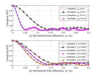
Figure 3: (a) Temporal ACF with different velocities at Rx side (b) Temporal ACF with different carrier frequencies ($\beta_{A}^{T}$=$\pi$/10, $\beta_{A}^{R}$=$\pi$/12, $\alpha_{A}^{T}$=$\pi$/10, $\alpha_{A}^{R}$=$\pi$/12, $\lambda_{G}$=20/m, $\lambda_{R}$=1/m, $D_{c}^{A}$=40 m).

IV-B The Space CCF

Fig. 4 illustrates the space CCF. The measurement was conducted in a campus environment at 2.6 GHz carrier frequency with 128 antenna elements ULA at BS side [18]. The simulation result is consistent with the measurement, which validated the presented model.

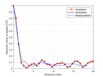
Figure 4: Absolute value of space CCF at different antenna spacings at the BS side ($f_{c}$=2.6 GHz, $M_{T}$=128, $M_{R}$=1, $\beta_{A}^{T}$=$\pi$/10, $\beta_{A}^{R}$=$\pi$/12, $\alpha_{A}^{T}$=$\pi$/10, $\alpha_{A}^{R}$=$\pi$/12, $\delta_{T}$=$\lambda/2$, $\lambda_{G}$=20/m, $\lambda_{R}$=1/m, $D_{c}^{S}$=40 m, NLOS).

IV-C The FCF

The FCF is shown in Fig. 5. The channel with different cluster azimuth spread values 3, 5, and 7 has different coherence bandwidths 680 MHz, 475 MHz, and 260 MHz, respectively. What should be noted that is the coherence bandwidth refers to the frequency separation when the FCF equals to 0.5. The above phenomenon indicates that the larger cluster azimuth spreads will reduce the correlation of the channel.

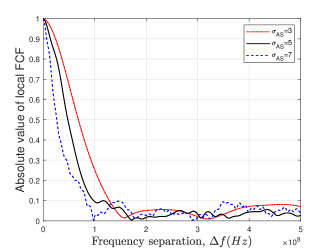
Figure 5: Absolute value of FCF with different cluster azimuth spreads ($f_{c}$=28 GHz, $\beta_{A}^{T}$=$\pi$/10, $\beta_{A}^{R}$=$\pi$/12, $\alpha_{A}^{T}$=$\pi$/10, $\alpha_{A}^{R}$=$\pi$/12, $\delta_{T}$=$\lambda/2$, $\lambda_{G}$=20/m, $\lambda_{R}$=1/m).

IV-D STF Cluster Evolution

Cluster evolutions in STF domain are shown in Fig. 6 (a), Fig. 6 (b), and Fig. 6 (c). Different antennas at the same time instant and frequency, or the same antenna at different time instants and frequencies will see different clusters, which indicates the channel is non-stationary in STF domain.

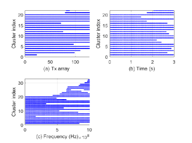
Figure 6: (a) Cluster evolution in space domain ($f_{c}$=5.3 GHz, $M_{T}$=128, $\delta_{T}$=$\lambda/2$, $D_{c}^{A}$=40 m) (b) Cluster evolution in time domain ($f_{c}$=5.3 GHz, $v_{R}$=15 m/s, $v_{T}$=0 m/s, $D_{c}^{S}$=40 m) (c) Cluster evolution in frequency domain ($f_{c}$=38 GHz, $v_{R}$=15 m/s, $v_{T}$=0 m/s).

IV-E The SVS

Fig. 7 illustrates the cumulative distribution functions (CDFs) of SVSs of simulation results and measurement in [19]. The channel measurement was performed in indoor scenario at 1.4725 GHz with a virtual 128-element ULA. The simulation results agree with the measurement data. When $M_{T}$ gradually increases to 128, the SVS gradually decreases to below 1 dB. The above phenomenon manifests that the channel becomes more and more stable, and the channel vectors among users become approximately orthogonal.

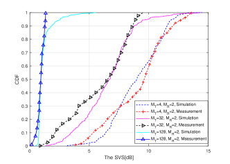
Figure 7: CDFs of SVSs with different numbers of antennas at Tx side ($f_{c}$=1.4725 GHz, $\beta_{A}^{T}$=$\pi$/3, $\beta_{A}^{R}$=$\pi$/4, $\alpha_{A}^{T}$=$\pi$/3, $\alpha_{A}^{R}$=$\pi$/3, $\delta_{T}$=$\lambda/2$, $\lambda_{G}$=20/m, $\lambda_{R}$=1/m, LOS).

IV-F Channel Capacity

The uplink sum-rates in the measured channels and the presented model are compared in Fig. 8 [20]. The simulation results are consistent with the measurement data. With the number of antennas increasing at BS side, the uplink sum-rates also increase within a certain SNR range.

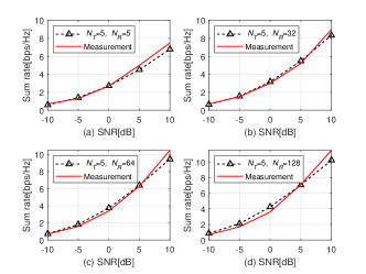
Figure 8: The uplink sum-rates with different numbers of antennas at Rx side ($f_{c}$=2.6 GHz, $\beta_{A}^{T}$=$\pi$/10, $\beta_{A}^{R}$=$\pi$/12, $\alpha_{A}^{T}$=$\pi$/10, $\alpha_{A}^{R}$=$\pi$/12, $\delta_{T}$=$\lambda/2$, $\lambda_{G}$=20/m, $\lambda_{R}$=1/m).

V Conclusions

The paper has proposed a general 3D massive MIMO GBSM for 6G communication systems. The presented model can support arbitrary velocities and trajectories at both Tx side and Rx side, which are equipped with URAs. Meanwhile, it has studied cluster evolution in STF domain to support STF non-stationary communication scenario. In addition, the spatial consistency of LSPs generation has been proved by using the method of parameter generation with spatial consistency. The simulations about temporal ACF, space CCF, FCF, SVS, and channel capacity are conducted. Analytical, simulation results, and measurements have also been compared to verify the validity of the channel model. The novel GBSM proposed in this paper will play a significant part in the development of 6G communication systems.

References

• [1] X.-H. You, C.-X. Wang, J. Huang, et al., β€œTowards 6G wireless communication networks: Vision, enabling technologies, and new paradigm shifts,” Sci. China Inf. Sci., vol. 64, no. 1, Jan. 2021, doi: 10.1007/s11432-020-2955-6.
• [2] C.-X. Wang, J. Huang, H. Wang, et al., ”6G Wireless Channel Measurements and Models: Trends and Challenges,” in IEEE Veh. Technol. Mag., vol. 15, no. 4, pp. 22-32, Dec. 2020.
• [3] H. Q. Ngo, E. G. Larsson, and T. L. Marzetta, β€œAspects of favorable propagation in massive MIMO,” in Proc. EUSIPCO, Lisbon, Sept. 2014, pp. 76–80.
• [4] J. Chen, β€œWhen does asymptotic orthogonality exist for very large arrays?” in Proc. IEEE GLOBECOM, Atlanta, GA, Dec. 2013, pp. 4146–4150.
• [5] Y. Lu, C. Tao, L. Liu, K. Liu, β€œSpatial characteristics of the massive MIMO channel based on indoor measurement at 1.4725 GHz,” IET Communications, vol. 12, no. 2, pp. 192–197, Nov. 2017.
• [6] J. Huang, C.-X. Wang, R. Feng, et al., β€œMulti-frequency mmWave massive MIMO channel measurements and characterization for 5G wireless communication systems,” IEEE J. Sel. Areas Commun., vol. 35, no. 7, pp. 1591–1605, July 2017.
• [7] J. Li and Y. Zhao, β€œChannel characterization and modeling for large-scale antenna systems,” in Proc. ISCIT, Incheon, Sept. 2014, pp. 559–563.
• [8] C. F. Lopez, C.-X. Wang, and R. Feng, β€œA novel 2D non-stationary wideband massive MIMO channel model,” in Proc. IEEE CAMAD, Toronto, ON, Oct. 2016, pp. 207–212.
• [9] C. F. LΓ³pez and C.-X. Wang, β€œNovel 3-D non-stationary wideband models for massive MIMO channels,” IEEE Trans. Wireless Commun., vol. 17, no. 5, pp. 2893–2905, May 2018.
• [10] S. Wu, C.-X. Wang, e. M. Aggoune, M. M. Alwakeel and Y. He, β€œA non-stationary 3-D wideband twin-cluster model for 5G massive MIMO channels,” IEEE J. Sel. Areas Commun., vol. 32, no. 6, pp. 1207–1218, June 2014.
• [11] S. Wu, C.-X. Wang, e. M. Aggoune, et al., β€œA general 3-D non-stationary 5G wireless channel model,” IEEE Trans. Commun., vol. 66, no. 7, pp. 3065–3078, July 2018.
• [12] J. Bian, C.-X. Wang, X. Gao, X.-H. You, and M. Zhang, β€œA general 3D non-stationary wireless channel model for 5G and beyond,” IEEE Trans. Wireless Commun., accepted for publication.
• [13] H. Wu, S. Jin, and X. Gao, β€œNon-stationary multi-ring channel model for massive MIMO systems,” in Proc. WCSP, Nanjing, Oct. 2015, pp. 1–6.
• [14] S. Wu, C.-X. Wang, H. Haas, et al., β€œA non-stationary wideband channel model for massive MIMO communication systems,” IEEE Trans. Wireless Commun., vol. 14, no. 3, pp. 1434–1446, Mar. 2015.
• [15] L. Wang, J. Chen, X. Yang, N. Ma and P. Zhang, β€œA 3D ellipsoid model for isotropic and non-isotropic scatterers co-existing massive MIMO channels,” in Proc. IEEE WCNCW, Marrakech, Morocco, Apr. 2019, pp. 1–6.
• [16] Y. Liu, C.-X. Wang, J. Huang, J. Sun and W. Zhang, β€œNovel 3-D nonstationary mmWave massive MIMO channel models for 5G high-speed train wireless communications,” IEEE Trans. Veh. Technol., vol. 68, no. 3, pp. 2077–2086, Mar. 2019.
• [17] A. Paulraj, R. Nabar, and D. Gore, Introduction to Space–Time Wireless Communications. Cambridge, U.K.: Cambridge Univ. Press, 2003.
• [18] S. Payami and F. Tufvesson, β€œChannel measurements and analysis for very large array systems at 2.6 GHz,” in Proc. EUCAP, Prague, Mar. 2012, pp. 433–437.
• [19] Q. Li, L. Liu, C. Tao, et al., β€œPerformance analysis of a massive MIMO system in indoor scenario,” in Proc. ISAPE, Hangzhou, China, Dec. 2018, pp. 1–4.
• [20] X. Gao, M. Zhu, F. Rusek, F. Tufvesson, and O. Edfors, β€œLarge antenna array and propagation environment interaction,” in Proc. ASILOMAR, Pacific Grove, CA, Nov. 2014, pp. 666–670.