Curvit:
An open-source Python package to generate light curves from UVIT data

Abstract

Curvit is an open-source Python package that facilitates the creation of light curves from the data collected by the Ultra-Violet Imaging Telescope (UVIT) onboard AstroSat, India’s first multi-wavelength astronomical satellite. The input to Curvit is the calibrated events list generated by the UVIT-Payload Operation Center (UVIT-POC) and made available to the principal investigators through the Indian Space Science Data Center. The features of Curvit include (i) automatically detecting sources and generating light curves for all the detected sources and (ii) custom generation of light curve for any particular source of interest. We present here the capabilities of Curvit and demonstrate its usability on the UVIT observations of the intermediate polar FO Aqr as an example. Curvit is publicly available on GitHub at https://github.com/prajwel/curvit.

prajwelpj@gmail.com

1 January 20151 January 2015

12.3456/s78910-011-012-3 #### 000 0000 1– 1

1 Introduction

The Ultra Violet Imaging Telescope (UVIT; Tandon $et~{}al$. 2017a, Tandon $et~{}al$. 2017c), consisting of two co-aligned telescopes of aperture 375 mm each, is one of the payloads onboard AstroSat. AstroSat is India’s first multi-wavelength astronomical observatory, launched by the Indian Space Research Organisation (ISRO) on 28, September 2015 (Agrawal 2006). In addition to UVIT, there are three co-aligned X-ray payloads on AstroSat enabling simultaneous observation of a celestial source over a wide range of wavelengths from hard X-rays to the Ultraviolet (UV) band. UVIT, with a field of view of 28 arcminute diameter, can perform imaging and low-resolution slit-less spectroscopy. UVIT has a large number of filters and with selectable filters or gratings, simultaneous observations in far-ultraviolet (FUV, 1300-1800 Å), near-ultraviolet (NUV, 2000-3000 Å), and visible (VIS, 3200-5500 Å) channels are possible. Of the three channels, VIS channel is used only for aspect correction, while the NUV and FUV channels are used for science observations. The detectors used in all the three channels are intensified CMOS imagers with 512$\times$512 pixels. The telescope pointing can drift up to $3^{\prime}$ over the night time of an orbit (duration can be up to a maximum of 1800 seconds) with a rate of $3^{\prime\prime}$/second. This drift of the satellite is estimated, as a function of time, using observations obtained with the VIS channel. In the normal mode of operations, observations are carried out in the full window mode (default mode, 512$\times$512 pixels) covering 28 diameter arcminute field resulting in a read rate of $\sim$28.7 frames/second. It is also possible to observe a partial field (that is selectable by the principal investigators (PIs) of the observing proposals) read at a higher rate. For example, the observation of a small window (100$\times$100 pixels) will provide 640 frames per second. The NUV and FUV images are generated by combining short exposure frames with shift and add algorithm. However, for bright fields, self drift correction of NUV data with NUV and FUV data with FUV is also possible. Two modes of operation exist in UVIT: (1) photon counting mode, achievable through high electron multiplication via high voltage to the microchannel plate of the intensified imager, in the case of NUV and FUV channels, where the intensified detectors record the X and Y positions of the photons on the detectors and their arrival times and (2) integration mode, achievable through a lower electron multiplication, for VIS channel where the readout consists of image frames with a time resolution of 1 second. In the final image obtained using photon counting mode, each detector pixel is mapped to 8$\times$8 sub-pixels by the centroiding of photon events with each sub-pixel having a plate scale of $0.416^{\prime\prime}$ (Hutchings $et~{}al$. 2007; Postma $et~{}al$. 2011). Due to the availability of time-tagged events in photon counting mode in FUV and NUV channels, it is possible to probe the time variability of observed sources in UV and generate light curves similar to other branches of high energy astronomy such as X-rays and $\gamma$-rays. UVIT has been performing as per specifications. More details and related calibration can be found in Tandon $et~{}al$. (2017b) and Tandon $et~{}al$. (2020).

The UVIT Payload Operation Center (POC) at the Indian Institute of Astrophysics (IIA) runs the UVIT Level-2 pipeline (UL2P; Ghosh et al. 2021, in preparation) on the Level-1 (L1) data, containing both spacecraft and observational data in FITS format, to produce science ready Level-2 (L2) data products. A description of UVIT data reduction is given in Postma & Leahy (2017) as well as Ghosh et al. (2021). The UVIT-POC processed L1 and L2 data are made available to the PIs of the observations through the ISRO Indian Space Science Data Center (ISSDC). The L2 data contains (i) orbit-wise calibrated events list after corrections for the drift of the spacecraft, flat field, and distortion (ii) orbit-wise science ready images in detector coordinate and world coordinate systems and (iii) combined images that belong to a single pointing, wherein observations in a particular filter carried out over many orbits in a particular pointing are combined. L2 data from ISSDC are science ready products, and the PIs can directly carry out their photometric, spectroscopic or imaging analysis. Alternatively, PIs willing to do a custom analysis of their observations can also do so, using UL2P, along with the CALDB (that contains the calibration data files) and the CATALOG (that contains the catalogues for astrometry) downloadable from ISSDC, UVIT-POC or the AstroSat Science Support cell.

Time variable phenomenon can be studied naturally using the ”photon counting mode” of operation for the UV bands of image acquisition by UVIT. In principle, in the full window mode observations with UVIT, one can study time-varying phenomenon with a time resolution as low as 66 msec in both the UV bands. Even higher time resolution is possible with smaller window observations (for example, $\sim$3 msec in 100$\times$100 pixels window). Studies of such high-resolution events will open up a new avenue of research in UV Astronomy, and for such studies, software tools are required to generate the light curves directly from the events list. The motivation is therefore to develop a software tool, that has the ability to create light curves from the events list. Here we present Curvit, an open-source Python package designed to create light curves from UVIT L2 events list. Curvit makes use of the functionalities available in other open-source Python packages such as Astropy (Astropy Collaboration $et~{}al$. 2013; Astropy Collaboration $et~{}al$. 2018), NumPy (Harris $et~{}al$. 2020), Matplotlib (Hunter 2007), Photutils (Bradley $et~{}al$. 2020, and Scipy (Virtanen $et~{}al$. 2020). The availability of this tool to the PIs of UVIT will also avert the cumbersome task of first creating images of small time-bins and then doing the photometry of the target to generate light curves. Section 2 contains a short summary of the L2 products at ISSDC. In Sections 3 and 4, we describe the functionalities and working of the tool. In the final section, we demonstrate the usefulness of the tool by generating the light curve of intermediate polar FO Aquarii (FO Aqr), observed under the guaranteed time and now open for public after the lock-in-period.

2 UVIT data products at ISSDC

The UVIT data is available at ISSDC AstroBrowse website. Both L1 and L2 data of UVIT are available as compressed files at the archive. L2 products are organised into two categories: individual datasets (single orbit for a filter and window; see Table 1), and combined datasets over all the orbits (for a single filter and window; see Table 2). The UVIT filters are given in Table 3.

Table 1: Details of the data products sent to ISSDC for each orbit of observation done in a particular window-size and filter.

Product	Description	RAS VIS∗		RAS NUV∗		Total
		NUV	FUV	NUV	FUV
Sky Image (Instrument coordinates)	4800$\times$4800 sub-pixel2 FITS image	1	1	1	1	4
Sky Image (Astronomical coordinates)	4800$\times$4800 sub-pixel2 FITS image	1	1	1	1	4
Exposure Map (Astronomical coordinates)	4800$\times$4800 sub-pixel2 FITS image	1	1	1	1	4
Error Map (Astronomical coordinates)	4800$\times$4800 sub-pixel2 FITS image	1	1	1	1	4
Photon Events List	FITS binary table	1	1	1	1	4
RAS file	FITS binary table	1		1		2

^∗The above file structure corresponds to the ideal case when VIS, NUV, and FUV are configured by the PI. In the event of VIS not being configured, the files generated using the relative aspect series (RAS) obtained from VIS data will be missing. Similar is the case for NUV.

Table 2: Details of the combined data products sent to ISSDC. The observations carried out over the entire pointing are combined filter wise.

Product	Description	RAS VIS		RAS NUV		Total
		NUV	FUV	NUV	FUV
Sky Image – A∗ (Astronomical coordinates)	4800$\times$4800 sub-pixel2 FITS image	1	1	1	1	4
Sky Image – B$ (Astronomical coordinates)	4800$\times$4800 sub-pixel2 FITS image	1	1	1	1	4
Exposure Map† (Astronomical coordinates)	4800$\times$4800 sub-pixel2 FITS image	1	1	1	1	4
Error Map† (Astronomical coordinates)	4800$\times$4800 sub-pixel2 FITS image	1	1	1	1	4

^∗Sky image – A: The astrometric accuracy of this image is limited to the accuracy of knowledge of the spacecraft aspect, which is typically around 2-3 arcmin.

^$Sky image – B: This is the final image generated after astrometry which may or may not be successful. When the astrometry is successful, the accuracy in aspect is typically 3 arcsec. When the astrometry is not successful, this image is a copy of Sky image – A. The information about astrometry being successful or unsuccessful is available in the header of the FITS images.

^†They correspond to the co-ordinate system of Sky image – B.

Table 3: The UVIT filters in VIS, NUV and FUV channels.

VIS			NUV			FUV
Filter ID	Old filter name	New filter name	Filter ID	Old filter name	New filter name	Filter ID	Old filter name	New filter name
F1	VIS3	V461W	F1	Silica - 1	N242W	F1	CaF2 - 1	F148W
F2	VIS2	V391M	F2	NUVB15	N219M	F2	BaF2	F154W
F3	VIS1	V347M	F3	NUVB13	N245M	F3	Sapphire	F169M
F4	ND1	V435ND	F4	Grating		F4	Grating - 1
F5	BK7	V420W	F5	NUVB4	N263M	F5	Silica	F172M
			F6	NUVN2	N279N	F6	Grating - 2
			F7	Silica - 2	N242Wa	F7	CaF2 - 2	F148Wa

3 Curvit Workflow

Curvit is an open-source Python package to produce light curves from UVIT data. The events list from the official UVIT L2 pipeline (version 6.3 onwards) is required as an input to the package. Curvit has two functions for light curve creation; makecurves and curve. Both the functions accept a single events list at a time which the user has to provide. We describe below each of these functions and its usage on the observation of the intermediate polar FO Aqr.

3.1 makecurves

The makecurves function of Curvit automatically detects sources from the events list and create light curves for all of them. The user will have a control on the number of sources detected automatically through the use of the detection threshold parameter. Two source detection methods are available; ’daofind’ and ’kdtree’. The user can select the preferred source detection method using the $detection\_method$ parameter (the default value is ’daofind’).

The ’daofind’ method detects sources in the following manner. It first creates a 4800$\times$4800 sub-pixel² image from the events list and a circular mask is applied to select the central $\sim$24 arcminute region. Sources are then detected using the daofind algorithm (Stetson 1987). Mean and standard deviation values of the background, required by daofind, are estimated by $Curvit$ itself and the user can control the number of sources detected using the $threshold$ parameter. Pixels in the image that have the events greater than the threshold times the standard deviation of the background will be detected.

The ’kdtree’ method works as follows. A source is characterised by a cloud of events around its centroid. Therefore, to detect sources, the events are projected onto a two-dimensional Cartesian grid (with one grid cell being of 1 sub-pixel² size), and the grid cells are sorted based on the number of events falling in each cell. Since a single source can occupy multiple grid cells, a nearest neighbour search using kdtree algorithm is performed to remove grid cells belonging to the same source (Maneewongvatana & Mount 1999). This method may not work properly on crowded fields. But in non-crowded fields, the method can detect all the sources present in the events list. However, the user may limit the number of sources to be detected using the parameter $how\_many$. Also, the aperture radius that is used to count the source events (through $radius$) and the size of the time bin to generate the light curves (using the parameter $bwidth$) can be controlled by the user.

The function makecurves generates light curves for each detected sources that depend on the threshold set by the user in terms of decreasing order of brightness. The operation of the function is summarised in Fig. 1.

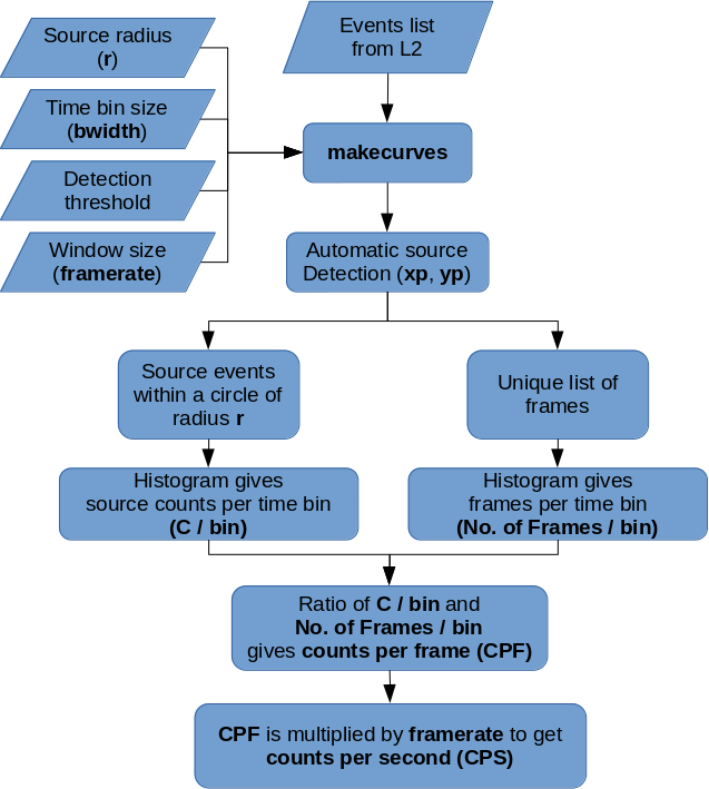
Figure 1: Flowchart for the function makecurves in Curvit.

3.2 curve

The function curve is similar to makecurves, with the exception that it generates light curve for a single user-defined source (through $xp$ and $yp$ parameters). Here also, the user can specify the source aperture radius and the binning time. Its operation is summarised in the Fig. 2.

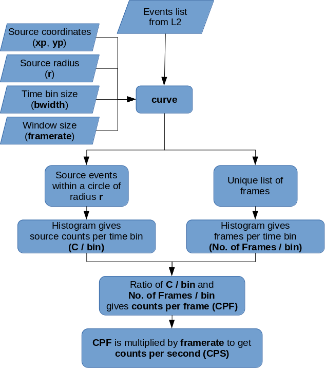
Figure 2: Flowchart for the function curve in Curvit.

4 Light curve Creation

From the events list FITS table, the columns ’Fx’, ’Fy’, ’MJD_L2’, and ’EFFECTIVE_NUM_PHOTONS’ (hereafter ENP) are used by Curvit (see Table 4). However, the events list FITS table has more columns than the ones given in Table 4. Each row of the table characterises a single event defined by X and Y Cartesian coordinate positions (’Fx’ and ’Fy’) with an associated time value (’MJD_L2’). For the L2 data available from ISSDC, ’MJD_L2’ provides only an approximate absolute time, good to $\sim$1 second. The time values in ’MJD_L2’ column increment as the frame number (as denoted in the ’FrameCounts’ column of events list) changes. Therefore, ’MJD_L2’ column can be considered as a proxy for ’FrameCounts’ column. ENP column stores the ’counts/second’ contribution from that specific event (row of the table) after including instrumental correction like flat-field across the detector (Ghosh et al. 2021, in preparation). In the methods mentioned below, each event is weighted as per the corresponding ENP value.

Table 4: Sample events list that show only the columns used by Curvit.

Frame
Counts	Fx	Fy	ENP	MJD_L2
…	…	…	…	…
3	2461.9	2918.0	28.5	213453019.048
3	3139.5	3651.2	25.6	213453019.048
4	875.9	2924.2	23.8	213453019.084
4	1444.0	3605.5	23.7	213453019.084
4	2166.7	3934.6	24.8	213453019.084
5	3355.4	1229.8	25.6	213453019.120
5	3216.9	1497.7	26.3	213453019.120
5	2798.5	3836.8	25.7	213453019.120
6	3113.4	2230.7	27.5	213453019.156
6	4367.8	2483.6	20.7	213453019.156
…	…	…	…	…

For a given source coordinate position, it is possible to define an aperture of some radius in the detector coordinate system (x,y) and select only those events (rows of the table) which fall inside the aperture. Thus, a subset table can be created from the original table. Here, the term original table is used to refer to the input events list table. The subset table will have only those events of the original table, that is assumed to be solely coming from the source. We will refer to the time values (equivalent to frame numbers) in the subset table as subset-time. Also, a separate array of unique time values is created from the original table. We will call this array as original-time.

Using the resultant two arrays of time (subset-time and original-time), two separate histograms are created. The number of bins (same for both histograms) to be used is determined from the user-provided bin width (see Appendix A). For subset-time, the histogram can be interpreted as the number of events per bin coming from the source. Whereas histogram of original-time should ideally give a constant value per bin. For example, if bin width is set to 1 second, one should always get $\sim$28.7 frames per second at all the bins for 512$\times$512 mode. However, if some frames are missing (for example, due to large telescope drift or missing data), this will be reflected as reduced values in the original-time histogram. Therefore correction for missing frames is carried out using the original-time histogram (see Appendix B for a detailed explanation).

By taking the ratio of two histograms, counts per frame (CPF) array is obtained. CPF array is then multiplied by frame-rate ($\sim$28.7 for 512$\times$512 mode; the user may specify the frame-rate using the $framecount\_per\_sec$ parameter) to obtain the counts per seconds (CPS) array. Finally, the CPS array is plotted against time as the light curve. The user is advised to look for variability in sources within the central 20 arcminute region to reduce telescope drift effects.

4.1 Background, aperture, and saturation corrections

Estimation of background CPS can be obtained by manually specifying a background region ($x\_bg$ and $y\_bg$) and aperture size ($sky\_radius$). It is also possible in Curvit to automatically determine background count-rate. To do this, a two-dimensional (2D) histogram of events with 16$\times$16 sub-pixel² bin size is created. A mask is applied on the 2D histogram to select only the central $\sim$24 arcminute region. As opposed to a source, a background region will not have the crowding of events around some centroid and have a comparatively low number of events in a 2D histogram bin containing it. Also, the values of histogram bins containing background regions are assumed to be normally distributed. Therefore, the bins with sources are removed using sigma clipping of the 2D histogram values and locations of background histogram bins are randomly selected to estimate the mean sigma clipped background count-rate using an aperture size of $sky\_radius$.

The end-user has also the option to apply aperture and saturation corrections using $aperture\_correction$ and $saturation\_correction$ parameters. Depending on the size of the radius used, the measured CPF will change. This difference is represented as a table of encircled energy at radii from 1.5 - 95 sub-pixels for both UV channels in Tandon $et~{}al$. (2020). Cubic interpolation was used to create a continuous function mapping radius to encircled energy in the stipulated range. From the encircled energy, aperture-corrected CPF can be represented as follows,

$$\mbox{Aperture-corrected CPF}=\frac{\mbox{Measured CPF}\times 100}{\mbox{Encircled energy (\%)}}$$ (1)

Thus, aperture correction is applied to CPF values in each bin.

If the average photon rate per frame is not $\ll$ 1, the effects of saturation will make the measured CPF different from the real CPF by a value of RCORR. As long as the measured CPF is $<$ 0.6, RCORR can be estimated as below (Tandon $et~{}al$., 2017b),

$$\mbox{ICPF5}=-\ln(1-\mbox{Measured CPF})$$ (2)

$$\mbox{ICORR}=\mbox{ICPF5}-\mbox{Measured CPF}$$ (3)

$$\mbox{RCORR}=\mbox{ICORR}\times(0.89-(0.30\times\mbox{ICORR}^{2}))$$ (4)

$$\mbox{Real CPF}=\mbox{Measured CPF}+\mbox{RCORR}$$ (5)

Following the method above, saturation correction is applied to CPF values in each bin.

4.2 Zero event frames and centroid parity errors

When the total count-rate for the observed region is small, then there will be many frames with no events; as the total count-rate go down, the fraction of zero event frames go up. This can be modelled using Poisson statistics Tandon $et~{}al$. (2017b).

$$F0_{total}=\exp{(-X_{total})}$$ (6)

where $X_{total}$ is the CPF for the whole field of view and $F0_{total}$ is the fraction of frames with no events (see Fig. 3). For $X_{total}$ values above 4.6, the $F0_{total}$ is less than 1% and $F0_{total}$ is less than 5% for $X_{total}$ values above 3. Since original-time histogram is used to account for the missing frames, CPF values for the source will be overestimated depending on $X_{total}$ value.

Additionally, a small fraction of the events (less than 0.01%) can be lost due to centroid parity errors. Since both zero event frames and centroid parity errors are randomly distributed, any light curves with periodicity and/or high count-rate can be taken to be having true variability.

Figure 3: Fraction of frames with no events as a function of total counts per frame.

5 Test on sample data

We took the publicly available L2 data (UL2P version 6.3) of FO Aqr (observation ID: G06_084T01_9000000710) from the ISSDC AstroBrowse website. As an example, the Curvit software was run on L2 events lists that correspond to observations with the FUV filter F148W to create light curves. Using makecurves function with the detection threshold value of 4, six sources were automatically detected and Curvit generated light curves for all of them (Fig. 5). they are labelled as (a) to (f) in Fig. 4. An aperture radius of 6 sub-pixels (2.5 arcseconds) and time bin of 50 seconds was used. The observed variance ($\Sigma^{2}$) of each of the light curves in Fig. 5 is due to contributions from intrinsic source variability and measurement uncertainty. In the event of the source being non-variable, the contribution of source variability to the observed variance is zero. Therefore variance becomes equal to the average value of squared errors ($\sigma^{2}$) of the light curve points. For each light curve, we calculated the variance and the mean of squared errors in the points and the ratio R = $\Sigma^{2}/\sigma^{2}$. For non-variable sources, this ratio R will be close to unity, and a source is considered variable if R is much larger than unity. The values of R calculated for the light curves of all the sources is given in Table 5.

We also calculated the normalised excess variance, $F_{var}$, for the light curves to test the significance of their variations following Rani $et~{}al$. (2019). For variable sources, $F_{var}$ will have a real and positive value (see Table 5). It is evident from Table 5 that only for the source (a), namely FO Aqr, (i) the ratio R is much larger than unity and (ii) $F_{var}$ is much larger than the error in $F_{var}$. These indicate that the larger variance of the source (a) is due to the intrinsic variability of the source. Though sources (c) and (d) have real and positive $F_{var}$ values, and R greater than unity, for (c) the error in $F_{var}$ is much larger than $F_{var}$ itself and for (d) $F_{var}$ is not that significant considering its error. Thus from the light curves of sources (a) to (f), statistical tests confirm that only source (a) is variable. We note that the light curves of the sources presented here pertain to one orbit of data and such an analysis of one orbit data can only pick out short-period variables and will miss out long-period variables. Therefore, for sources where the period of variability is much longer than the one orbit data presented here, it is advisable to generate light curves for the complete observation (that can spread over many orbits), which might amount to carrying out photometry on each orbit wise images and then check for the presence of variability.

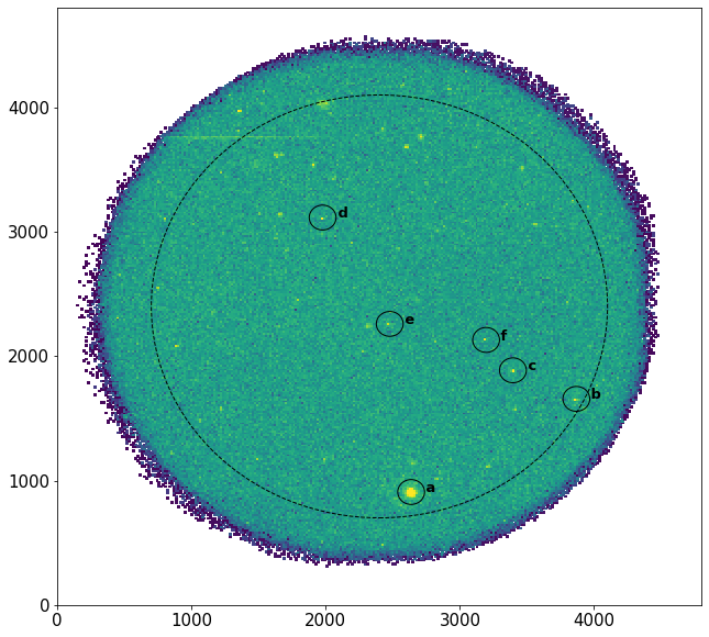
Figure 4: The sources that are detected within the central 24 arcminute region (dashed circle) by makecurves.

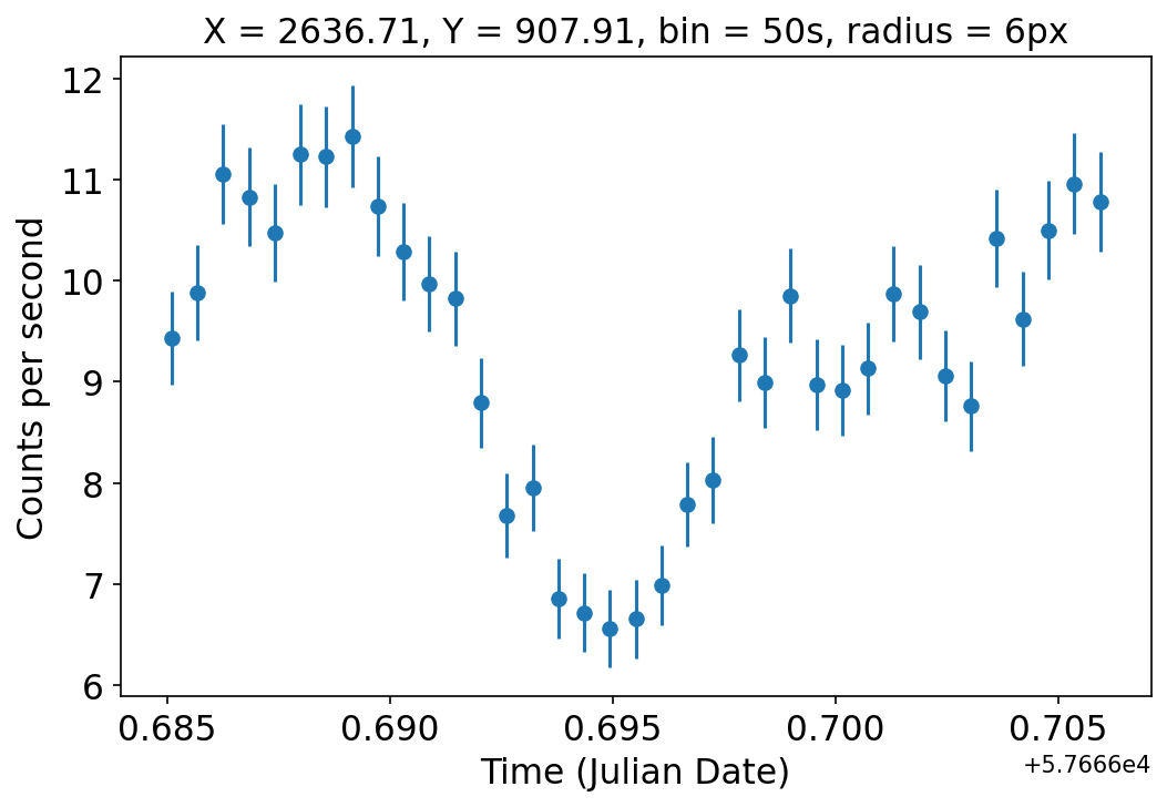
(a)

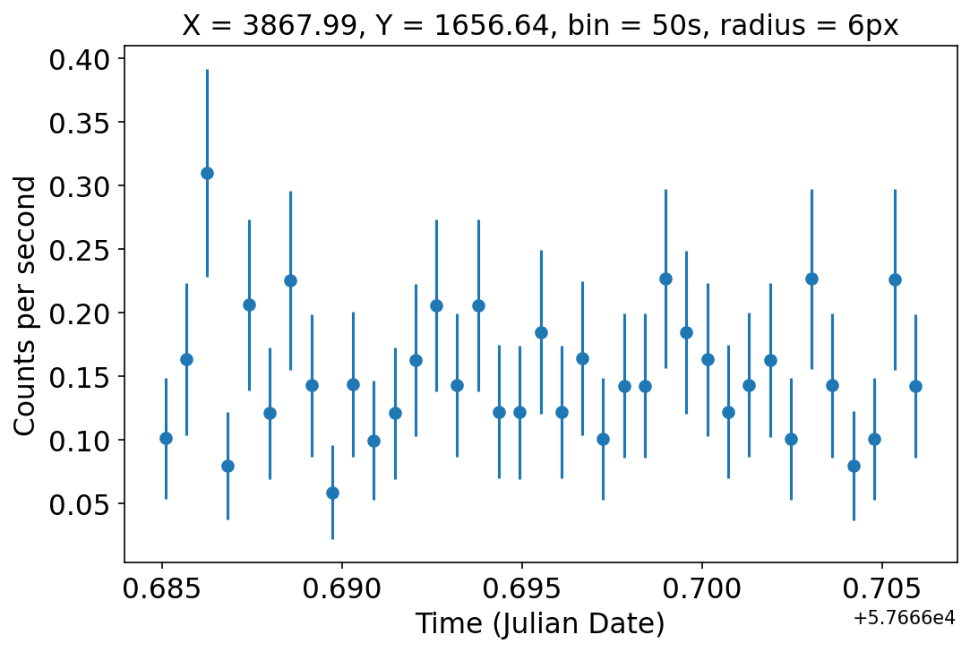
(b)

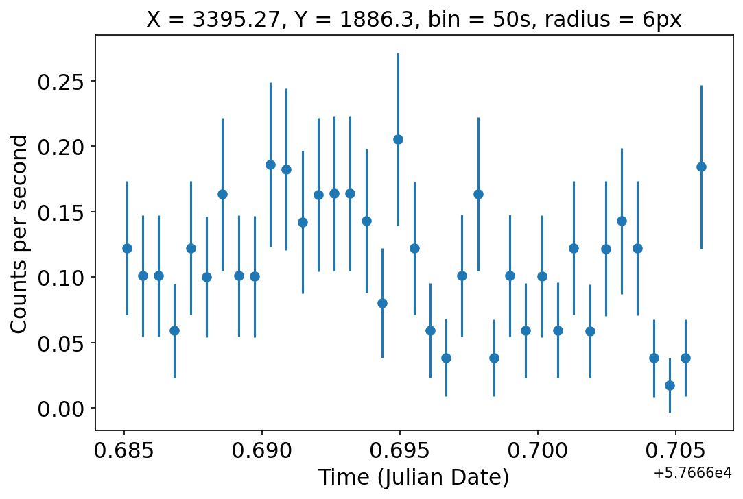
(c)

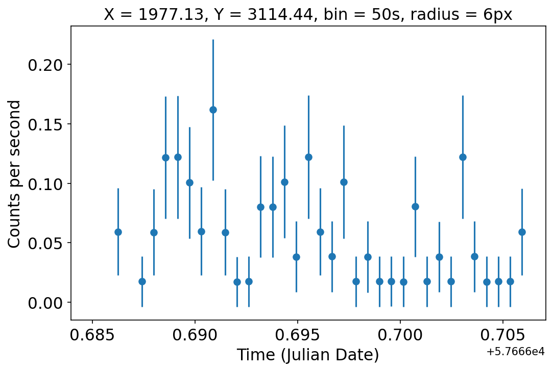
(d)

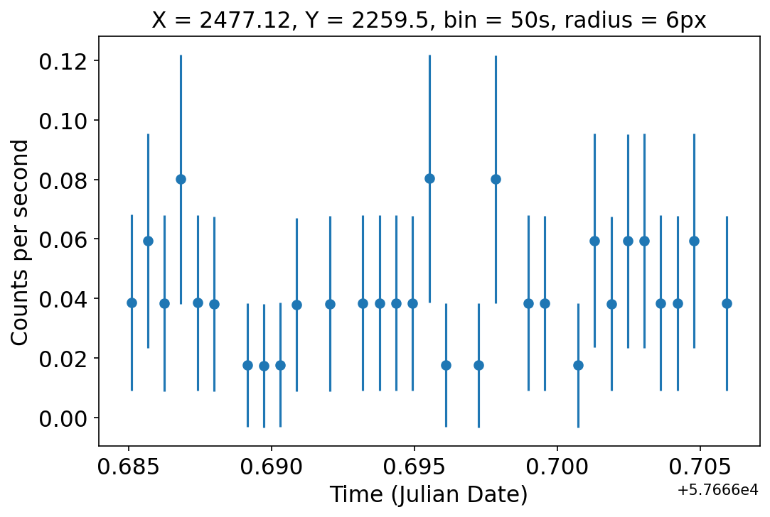
(e)

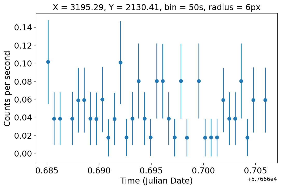
(f)

Figure 5: Light curves generated by the makecurves function in Curvit.

Table 5: Variability measure of detected sources.

Source	$\Sigma^{2}/\sigma^{2}$	$F_{var}$	$F_{var}$ error
a	11.87	0.14	0.02
b	0.88	-	-
c	1.01	0.04	0.58
d	1.39	0.38	0.16
e	0.35	-	-
f	0.61	-	-

6 Conclusion

The UVIT-POC at IIA processes the L1 data for UVIT received from ISSDC, generates science ready L2 products and transfers both the corrected L1 and L2 products to ISSDC for archival and dissemination to the PIs. Among the various files sent to ISSDC is the calibrated orbit-wise photon events list. The Curvit software tool presented here is a standalone package in Python that can generate light curves from the events list. This overcomes the cumbersome task of first creating images at any time resolution from the events list and then doing photometry on the images to generate the light curves of any desired object in the observed field. The Curvit package has the capability to (1) generate light curves for all the sources in the observed field detected above a threshold for any time binning given by the user and (2) generate light curve for any particular source at any time binning desired by the user. We have also shown an example light curve of a target FO Aqr observed by UVIT. Curvit is publicly available on GitHub at https://github.com/prajwel/curvit.

Appendix A To estimate the number of bins

To calculate the number of bins, the very first and last values of the original-time array is taken to estimate the width of the time array. Then, the time array width is divided by the bin width, and integer part of the resultant value is taken as the number of bins.

$$\mbox{Number of bins}=\frac{\mbox{original time\ width}}{\mbox{bin width}}$$ (7)

Appendix B Missing frame correction

Assume that an ideal non-variable source has a flux of 0.1 CPF (or $\sim$2.87 CPS for 512$\times$512 mode). If the bin width were set to 1 second, then the subset-time histogram would be as follows.

[2.87, 2.87, 2.87, 2.87, 2.87, 2.87,…]

However, if some of the frames vis-a-vis rows are missing from events list FITS table, we might get an array as given below.

[2.87, 2.53, 1.01, 2.84, 1.94, 2.87,…]

A false variability can be inferred from the above array. To overcome this, the original-time histogram is used. The missing frames will be reflected as a reduced number of events per bin in original-time histogram. For the case above, the original-time histogram would be as follows.

[28.7, 25.3, 10.1, 28.4, 19.4, 28.7,…]

By taking the ratio of two histograms, the real light curve in CPF is obtained as follows.

[0.1, 0.1, 0.1, 0.1, 0.1, 0.1,…]

CPF is then converted to CPS by multiplying with the frame-rate ($\sim$28.7 for 512$\times$512 mode).

References

- Agrawal (2006) Agrawal, P. 2006, Advances in Space Research, 38, 2989 , spectra and Timing of Compact X-ray Binaries
- Astropy Collaboration . (2013) Astropy Collaboration, Robitaille, T. P., Tollerud, E. J., . 2013, aap, 558, A33
- Astropy Collaboration . (2018) Astropy Collaboration, Price-Whelan, A. M., SipHocz, B. M., . 2018, aj, 156, 123
- Bradley . (2020) Bradley, L., Sipőcz, B., Robitaille, T., . 2020, astropy/photutils: 1.0.1, doi:10.5281/zenodo.4049061
- Harris . (2020) Harris, C. R., Millman, K. J., van der Walt, S. J., . 2020, Nature, 585, 357–362
- Hunter (2007) Hunter, J. D. 2007, Computing In Science & Engineering, 9, 90
- Hutchings . (2007) Hutchings, J. B., Postma, J., Asquin, D., & Leahy, D. 2007, Publications of the Astronomical Society of the Pacific, 119, 1152
- Maneewongvatana & Mount (1999) Maneewongvatana, S., & Mount, D. M. 1999, in Center for geometric computing 4th annual workshop on computational geometry, Vol. 2, 1–8
- Postma . (2011) Postma, J., Hutchings, J. B., & Leahy, D. 2011, Publications of the Astronomical Society of the Pacific, 123, 833
- Postma & Leahy (2017) Postma, J. E., & Leahy, D. 2017, Publications of the Astronomical Society of the Pacific, 129, 115002
- Rani . (2019) Rani, P., Stalin, C., & Goswami, K. D. 2019, Monthly Notices of the Royal Astronomical Society, 484, 5113
- Stetson (1987) Stetson, P. B. 1987, Publications of the Astronomical Society of the Pacific, 99, 191
- Tandon . (2017a) Tandon, S., Stalin, C., Subramaniam, A., Ghosh, S., & Hutchings, J. 2017a, Current Science (Bangalore), 113, 583
- Tandon . (2017b) Tandon, S. N., Subramaniam, A., Girish, V., . 2017b, The Astronomical Journal, 154, 128
- Tandon . (2017c) Tandon, S. N., Hutchings, J. B., Ghosh, S. K., . 2017c, Journal of Astrophysics and Astronomy, 38, 28
- Tandon . (2020) Tandon, S. N., Postma, J., Joseph, P., . 2020, The Astronomical Journal, 159, 158
- Virtanen . (2020) Virtanen, P., Gommers, R., Oliphant, T. E., . 2020, Nature Methods, 17, 261