Old but Gold: Reconsidering the value of
feedforward learners for software analytics

Abstract.

There has been an increased interest in the use of deep learning approaches for software analytics tasks. State-of-the-art techniques leverage modern deep learning techniques such as LSTMs, yielding competitive performance, albeit at the price of longer training times.

Recently, Galke and Scherp (2021) showed that at least for image recognition, a decades-old feedforward neural network can match the performance of modern deep learning techniques. This motivated us to try the same in the SE literature. Specifically, in this paper, we apply feedforward networks with some preprocessing to two analytics tasks: issue close time prediction, and vulnerability detection. We test the hypothesis laid by Galke and Scherp (2021), that feedforward networks suffice for many analytics tasks (which we call, the “Old but Gold” hypothesis) for these two tasks. For three out of five datasets from these tasks, we achieve new high-water mark results (that out-perform the prior state-of-the-art results) and for a fourth data set, Old but Gold performed as well as the recent state of the art. Furthermore, the old but gold results were obtained orders of magnitude faster than prior work. For example, for issue close time, old but gold found good predictors in 90 seconds (as opposed to the newer methods, which took 6 hours to run).

Our results supports the “Old but Gold” hypothesis and leads to the following recommendation: try simpler alternatives before more complex methods. At the very least, this will produce a baseline result against which researchers can compare some other, supposedly more sophisticated, approach. And in the best case, they will obtain useful results that are as good as anything else, in a small fraction of the effort.

To support open science, all our scripts and data are available on-line at https://github.com/fastidiouschipmunk/simple.

1. Introduction

As modern infrastructure allows for cheaper processing, it has inevitably led to the exploration of more complex modeling. For example, many software engineering researchers are now using deep learning methods (Gao et al, 2020; Hoang et al, 2019; Liu et al, 2019; Zhou et al, 2019, 2019; Chen and Zhou, 2018; Lee et al, 2020).

One problem with deep learning is that it can be very slow to run (Jiang and Agrawal, 2018; Le et al, 2011; Martens et al, 2010). For example, for the case study of this paper, we estimate that we would need 6 years of CPU time. Such long runtimes can complicate many aspects of the scientific process (e.g. initial investigations, subsequent attempts at reproduction).

Accordingly, this paper checks if anything simpler than deep learner can handle SE tasks. Outside of SE there is some suggestion that deep learning researchers have rushed on too far and have overlooked the benefits of simpler neural architectures. For example, Galke and Scherp (2021) offer an Old but Gold hypothesis; i.e. that in their rush to try new algorithms, researchers have overlooked the advantages of more traditional approaches. In their work, Galke and Scherp (2021) showed that for image classification, simple, decades-old feedforward networks (described in §3.2) can perform as well as modern deep learning techniques, at some small fraction of the computational cost.

Since deep learning is widely used in software engineering, it seems prudent to check for old but gold effects in SE applications. In this paper we explore two standard software analytics problems using older-style neural networks as well as the latest state-of-the-art deep learning algorithms.

The experiments of this paper show that simpler methods than prior work are better for some domains. Specifically, a simple extension to a 1980s-style feedforward neural network, which we call “SIMPLE”, runs much faster than prior work (90 seconds versus 6 hours for issue lifetime prediction). Since they run faster, feedforward networks are more amenable to automatic tuning methods. Such tuning requires multiple runs of a learner (Tantithamthavorn et al, 2016; Fu et al, 2016; Agrawal and Menzies, 2018; Agrawal et al, 2019) and so the faster the learner, the more we can tune it (which we do in this paper). Hence SIMPLE’s feedforward networks out-perform the prior work in issue lifetime prediction since the latter is fundamentally hard to customize to the task at hand.

The rest of this paper is structured as follows. §2 presents the necessary background and §2.2 discusses the SE task under consideration. §4 discusses our proposed approach. Then, in §5, we show our results. We discuss the threats to the validity of our study in §6. In §8 we conclude that before analysts try very sophisticated (but very slow) algorithms, they might achieve better results, much sooner, by applying hyper-parameter optimization to simple (but very fast) algorithms.

1.1. Preliminaries

Before beginning, just to say the obvious, we note the experiments of this paper are based on two case studies. Hence, they do not show that all deep learners can be replaced by faster and simpler methods.

That said, we would argue that this paper is at the very least arguing for a methodological change in how software analytics researchers report their deep learning results. Deep learners (or, indeed, any data mining results) should be compared to a simpler baseline method (in our case, feedforward networks) and also be adjusted via automatic tuning algorithms. The experience of this paper is that such a baseline + tuning analysis can lead to challenging and insightful results.

2. Case Studies

Before going into algorithmic details, this paper first presents the two domains that will be explored by those algorithms.

2.1. Vulnerability Detection

Cyber attacks often rely on software vulnerabilities, i.e., unintentional security flaws in software that can be taken advantage of to obtain unauthorized access, steal data, etc. As of writing this paper, the Common Vulnerabilities and Exposures (CVE) database contains over 165,000 records of vulnerabilities. This number only counts the registered vulnerabilities, and not unknown (or “zero-day”) vulnerabilities. For the security of software systems and the data associated with them (for example, in SQL databases), it is critical that these vulnerabilities be discovered and patched. However, manually searching for vulnerabilities is a time-consuming task.

There are several existing solutions that attempt to automate this task (Viega et al, 2000; Grieco et al, 2016; Kim et al, 2017). However, these rely on significant human effort. Specifically, they rely on the use of human-generated features, which can take time, and be expensive (since skilled human time is expensive). Moreover, these approaches tend to either have too many false negatives (i.e., missed vulnerabilities), or too many false positives (i.e., a “learner” that blindly marks non-vulnerable code as a vulnerability). These issues make these techniques less useful in practice.

2.1.1. Algorithms for Vulnerability Detection

To tackle these two problems, deep learning solutions have been recently proposed. Li et al (2018a) propose VulDeePecker, a bidirectional LSTM (Hochreiter and Schmidhuber, 1997) technique. From an external perspective, their approach takes in program segments, trains a deep learner, and then uses it to detect vulnerable code. Because this approach relies on training on the code to generate vector representations (which the network then uses to make predictions), it can be slow to run. Zhou et al (2019) propose Devign, which instead uses graph neural networks (Kipf and Welling, 2016) to detect vulnerabilities. A graph neural network takes in a graph input, and uses “graph convolutions” to extract hierarchical features. These features can then be used to make predictions in the later layers of the network. The authors of Devign experiment with several graph representations of source code, and recommend a composite version of their approach. Based on our literature review, we assert that this is the state-of-the-art approach for vulnerability detection.

However, deep learning approaches themselves can have issues. The major one is that deep learners can be slow to run (Jiang and Agrawal, 2018; Le et al, 2011; Martens et al, 2010). The primary reason for this is the use of more modern deep learning techniques such as the above mentioned bidirectional LSTMs. While these certainly have a lot of representational capacity, they suffer from having orders of magnitude more parameters than simpler, feedforward networks, and therefore take longer to optimize.

In this paper, we take a similar approach to VulDeePecker in that we use a deep learning technique to transform code into a vector representation, and then use our simple feedforward networks for prediction. However, unlike their approach, we use an off-the-shelf code-to-vector transformation tool, code2vec (Alon et al, 2019). Because there is no training involved in using this model off-the-shelf, our runtimes are significantly faster, since only the feedforward networks need to be trained.

2.2. Predicting Bugzilla Issue Close Time

When programmers work on repositories, predicting issue close time has multiple benefits for the developers, managers, and stakeholders since it helps:

• Developers prioritize work;

• Managers allocate resources and improve consistency of release cycles;

• Stakeholders understand changes in project timelines and budgets.

• It is also useful to predict issue close time when an issue is created; e.g. to send a notification if it is predicted that the current issue is an easy fix.

We explore issue close time, for two reasons. Firstly, it is a well studied problem (Lee et al, 2020; Rees-Jones et al, 2017; Vieira et al, 2019; Akbarinasaji et al, 2018; Guo et al, 2010; Giger et al, 2010; Marks et al, 2011; Kikas et al, 2016; Habayeb et al, 2017). Secondly, recent work has proposed a state-of-the-art deep learning approach to issue close time prediction (see the DeepTriage deep learning systems from COMAD’19, described later in this paper (Mani et al, 2019)).

2.2.1. Traditional Algorithms for Predicting Issue Close Time

Most large software systems have a system to track bugs, or issues, in the product. These issues typically go through the same lifecycle, in which they transition across various states, including UNCONFIRMED and CLOSED, while also being assigned final states such as WONTFIX (Weiss et al, 2007).

To find prior work on predicting issue close time, we searched for papers in the last ten years (since 2010) in Google Scholar using keywords “bug fix time”, “issue close time”, and “issue lifetime”. Then, we filtered them according to the criterion that they must be published in a top venue according to Google Scholar metrics Software Systems. Finally, using engineering judgement, we added in systems that were recommended by reviewers of a prior draft of this paper. That search found several noteworthy systems:

• Guo et al (2010) use logistic regression on a large closed-source project (Microsoft Windows), to predict whether or not a bug will be fixed. Using regression analysis, they identified the factors that led to bugs being fixed or not fixed.

• Giger et al (2010) use decision trees to predict the bug-fix time for Mozilla, Eclipse, and GNOME projects. They divided their target class into two labels: fast and slow, to get a binary classification problem, and used the area under the ROC curve (AUC) metric as their evaluation criteria.

• Marks et al (2011) also used decision trees, but instead, use an ensemble method, i.e., random forests, on Eclipse and Mozilla data. Their motivation for using random forests, apart from the better performance as compared to standard decision trees, is the ability to extract the relative importance of features in the input data. They report accuracy scores of 63.8% and 67.2% on the Mozilla and Eclipse repositories respectively.

• At MSR’16, Kikas, Dumas, and Pfahl (Kikas et al, 2016) built time-dependent models for issue close time prediction using Random Forests with a combination of static code features, and non-code features to predict issue close time with high performance

• More recently, Habayeb et al (2017) reported in IEEE TSE’17 a prediction system based on hidden Markov chains. Like Giger et al (2010), they divided their target labels into fast and slow fix-times and experimented with different values of the number of hidden states of the hidden Markov model.

Based on the above, we assert that the two prior state-of-the-art non-neural methods in area used random forests and logistic regression. Hence we will we use these two systems as part of the following study.

2.2.2. Deep Learning and Issue Close Time

As to deep learning and issue close time prediction, two contenders for “state-of-the-art” are DASENet (Lee et al, 2020) and DeepTriage(Mani et al, 2019). The DASENet paper asserts that their algorithm defeats DeepTriage but, after much effort, we could not reproduce that result. Hence, for this study, we use DeepTriage since:

• It is a state-of-the-art deep learner that performs for lifetime prediction.

• It has been very recently published (2019);

• Its reproduction package allowed us to run that code on our machines.

• It uses datasets commonly used in the literature (Technical aside: we were tempted to use the dataset provided by Vieira et al (2019) for our deep learning baseline. However, their lack of prior benchmarks meant we could not provide a comparison to demonstrate the efficacy of our approach.)

From a technical perspective, DeepTriage is Mani et al (2019)’s extension of bidirectional LSTMs with an “attention mechanism”. A Long Short-Term Memory (LSTM) (Hochreiter and Schmidhuber, 1997) is a form of recurrent neural network that has additional “gate” mechanisms to allow the network to model connections between long-distance tokens in the input. Bidirectional variants of recurrent models, such as LSTMs, consider the token stream in both forward and backward directions; this allows for the network to model both the previous and the following context for each input token. Attention mechanisms(Bahdanau et al, 2014) use learned weights to help the network “pay attention” to tokens that are more important than others in a context. Prior to running DeepTriage, its authors recommend using a standard set of preprocessing techniques: pattern matching to remove special characters and stack traces, tokenization, and and pruning the corpus to a fixed length. Beyond these steps, they rely on the deep learner to perform automated feature engineering.

3. Algorithms

Having discussed the domains we need to explore, this paper now turns to how we will explore them.

For the purposes of exposition, we label divide this discussion on these algorithms into three groups:

• Older style Feedforward Networks

• Newer-style Deep Learners

• Hyperparameter optimizers, which we use to tune the parameters of Feedforward Networks and Deep learners

Note that the system we are calling SIMPLE is a combination of Feedforward Networks and Hyperparameter Optimization.

3.1. Feedforward Networks

Feedforward neural networks (LeCun et al, 2015) apply a general “activation function” at each node after performing the matrix multiplication of the weights with the inputs. These networks grew in popularity following the invention of the ReLU (rectified linear unit) function (Nair and Hinton, 2010), $f(x)=\max(0,x)$, which significantly improved the results of neural networks. Specifically, for a layer $i$, if the weight matrix is represented in matrix form as $W^{[i]}$, the bias terms (the constants) are represented by $b^{[i]}$, and the values of the activation function are represented as $a^{[i]}$, then $a^{[0]}=X$ and $z^{[i]}=W^{[i]T}a^{[i-1]}+b^{[i]}$ and $a^{[i]}=f(z^{[i]})$ where $X$ is the input matrix.

There are several activation functions; for brevity, we only discuss the ones relevant in this study. Following the advice of LeCun et al (2015), for binary and multi-classification problems:

• For the last layer of the network, this study uses Sigmoid(x) $=\frac{1}{1+e^{-x}}$ and Softmax(x) $=\frac{\exp(x_{k})}{\sum_{j=1}^{|x|}\exp(x_{j})}$ respectively.

• For the other layers, we use ReLU(x) $=\max(0,x)$.

3.2. Deep Learning

For the rest of this paper, the following distinction will be important:

• The algorithms DeepTriage and VulDeePecker (used for issue close time and vulnerability defection, respectively) are based on new neural network technology comprising extensive layers of reasoning, where layer $i$ organizes the inputs offered to layer $i+1$.

• Our SIMPLE method is based on old feedforward neural networks which is a technology that dates back decades. At each node of these networks, the inputs are multiplied with weights that are learned, and then an activation function is applied. The weights are learned by the backpropagation algorithm (Rumelhart et al, 1985).

The difference between these approaches can be understood via Figure 1. The older methods use just a few layers while the “deep” learners use many layers. Also, the older methods use a threshold function at each node, while feedforward networks typically use the ReLU function $f(x)=\max(0,x)$.

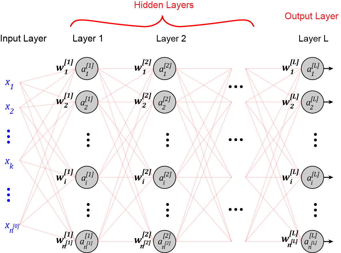
Figure 1. Illustration of a neural net model. Feedforward networks, such as those used in SIMPLE, have far fewer hidden layers than deep learners.

3.3. Hyperparameter Optimization

A common factor in all neural networks (feed-forward, deep learner, etc) is the architecture of the many layers of neural networks  (Goodfellow et al, 2016). In deep learning terminology, an “architecture” refers to the arrangement of nodes in the network and the connections between them, which dictates how the backpropagation algorithm updates the parameters of the model. Depending on the choice of the optimization algorithm (such as Adam  (Kingma and Ba, 2014)) and the architecture used, the model also has several hyper-parameters, such as the number of layers, the number of nodes in each layer, and hyper-parameters of the optimization algorithm itself (Brown et al, 2020).

The selection of appropriate hyper-parameters is something of a black art. Hence there exists a whole line of research called hyper-parameter optimization that explores automatic methods for finding these values.

For this study, we consider using two such optimizers: TPE (tree-structured Parzen estimators) from Bergstra et al. (Bergstra and Bengio, 2012; Bergstra et al, 2011) and DODGE from Agrawal et al. (Agrawal et al, 2019, 2021):

• TPE is a candidate hyper-parameter tuner since a December 2020 Google Scholar search for “Hyper-parameter optimization” reported that papers by Bergstra et al. (Bergstra and Bengio, 2012; Bergstra et al, 2011) on TPE optimization have more citations (2159 citations and 4982 citations) that any other paper in this arena.

• DODGE is another candidate hyper-parameter since, unlike TPE, it has been extensively tested on SE data sets. In 2019, Agrawal et al. (Agrawal et al, 2019) reported that for a range of SE problems (bad small detection, defect prediction, issue severity prediction) learners tuned by DODGE out-perform prior state-of-the art results (but a missing part of their analysis is that they did not study deep learning algorithms, hence, this paper).

How to choose between these algorithms? In 2021, Agrawal et al. (Agrawal et al, 2021) showed that DODGE is preferred over TPE for “intrinsically simple” data sets. Levina and Bickel (2004) argue that many datasets embedded in high-dimensional spaces can be compressed without significant information loss. They go on to say that a simple linear transformation like Principal Components Analysis (PCA) (Pearson, 1901) is insufficient, as the lower-dimensional embedding of the high-dimensional points are not merely projections. Instead, Levina and Bickel (2004) propose a method that computes the intrinsic dimensionality by counting the number of points within a distance $r$ while varying $r$. For notes on that computation, see Table 2

Table 1. Feedforward networks are controlled by these hyper-parameters.

Preprocessors: • StandardScaler : i.e. all input data set numerics are adjusted to $(x-\mu)/\sigma$. • MinMaxScaler (range = (0, 1)): i.e. scale each feature to $(0,1)$. • Normalizer (norm = randchoice([‘l1’, ‘l2’,‘max’])): i.e. normalize to a unit norm. • MaxAbsScaler (range = (0, 1)): scale each feature by its maximum absolute value • Binarizer (threshold = randuniform(0,100)), i.e., divide variables on some threshold

Hyper-parameters: • Number of layers • Number of units in each layer • Batch size (i.e., the number of samples processed at a time)

Intrinsic dimensionality (which we will denote as $D$) can be used to select an appropriate hyper-optimization strategy. Agrawal et al. (Agrawal et al, 2021). experiments show that DODGE beasts TPE for low dimensional data (when $D<8$) while TPE is the preferred algorithm for more complex data.

Table 2. Notes on intrinsic dimensionality.

Before presenting the mathematics of the Levina and Bickel (2004) measure, we offer a little story to explain the intuition behind this measure Consider a brother and sister who live in different parts of town. The sister lives alone, out-of-town, on a road running north-south with houses only on one side of the street. Note that if this sister tries to find company by walking: • Vertically up or down; • Or east or west then she will meet no one else. But if she walks north or south, then she might find company. That is, the humans in that part of town live in a one-dimensional space (north-south). Meanwhile, the brother lives downtown in the middle of a large a block of flats that is also oriented north-south. The brother is ill-advised to walk east-west since then they will fall off a balcony. On the other hand, if he : • Climbs up or down one storey • Or walks to the neighboring flats north or south then the brother might meet other people. That is to say, the humans in that block of flats effectively live in a two-dimensional space (north-south and up-down). To compute Levina’s intrinsic dimensionality, we create a 2-d plot where the x-axis shows $r$; i.e. how far we have walked away from any instance and the y-axis show $C(r)$ which counts how many more people we have meet after walking some distance $r$ way from any one of $n$ instances: $$y=C(r)=\frac{2}{n(n-1)}\sum\limits_{i=1}^{n}\sum\limits_{j=i+1}^{n}I\left[\lVert x_{i},x_{j}\rVert<r\right]$$ The maximum slope of $\ln C(r)$ vs. $\ln r$ is then reported as the intrinsic dimensionality. Note that $I[\cdot]$ is the indicator function (i.e., $I[x]=1$ if $x$ is true, otherwise it is 0); $x_{i}$ is the $i$th sample in the dataset. Note also that, as shown by Aggarwal et al (2001), at higher dimensions the distance calculations should use the $L_{1}$ norm, i.e., $\sum\lvert x_{i}\rvert$ rather than the $L_{2}$ norm, i.e., $\sqrt{\sum x_{i}^{2}}$.

Using the calculation methods of Agrawal et al. (Agrawal et al, 2021), we find that for our data:

$$\mathit{D(Firefox,\;Chromium,\;Eclipse)}=\{2.1,\;1.95,\;1.9\}$$

From this, we make two observations. Firstly, in a result that may not have surprised Levina et al., this data from Firefox, Chromium, Eclipse can be compressed w to just a few dimensions. Secondly, all our data can be found below the $D<8$ threshold proposed by Agrawal et al. (Agrawal et al, 2021). Hence, for this study, we use DODGE.

Compared to other hyper-parameter tuners, DODGE is a very simple algorithm that runs in two steps:

1. During an initial random step, DODGE selects hyper-parameters at random from Table 1. Each such tuning is used to configure a learner. The value of that configuration is then assessed by applying that learner to a data set. If ever a NEW result has performance scores near an OLD result, then a “tabu” zone is created around OLD and NEW configurations that subsequent random searches avoid that region of configurations.

2. In the next step, DODGE selects configurations via a binary chop of the tuning space. Each chop moves in the bounds for numeric choices by half the distance from most distant value to the value that produced the “best” performance. For notes on what “best” means, see §4.6.

Agrawal et al. recommend less than 50 evaluations for each of DODGE’s two stages. Note that this is far less than other hyper-parameter optimizations strategies. To see that, consider another hyper-parameter optimization approach based on genetic algorithms that mutate $P$ individuals over $G$ generations (and between each generation, individuals give “birth” to new individuals by crossing-over attributes from two parents). Holland (John, 1992) recommends P=G=100 as useful defaults for genetic algorithms. Those default settings implies that a standard genetic algorithm tuner would require $100*100=10,000$ evaluations.

Note that we also considered tuning DeepTriage, but that proved impractical:

• The DeepTriage learner used in this study can take up to six CPU hours to learn one model from the issue close time data. When repeated for 20 times (for statistically validity) over our (15) data sets, that means that using DODGE (using 42 evaluations) on DeepTriage would require over 8 years of CPU time.

• On the other hand, with 20 repeats over our datasets, DODGE with feedforward networks terminated in 26 hours; i.e. nearly 2,700 times faster than tuning DeepTriage.

4. Experimental Methods

4.1. Methods for Issue close time prediction

This section discusses how we comparatively evaluate different ways to do issue close time prediction. We explore three learners:

• DeepTriage: a state-of-the-art deep learner from COMAD’19 (Mani et al, 2019);

• Our SIMPLE neural network learner, described in §4.5;

• Non-neural approaches: random forest from  Marks et al (2011), and logistic regression from Guo et al (2010) (we present the better of the two results, where “better” is defined via the statistical methods of §4.7).

These learners will be studied twice:

• Once, with the default off-the-shelf settings for learners control parameters;

• Once again, using the settings found after some automatic tuning.

The original research plan was to present six sets of results:

planned = {L1,L2,L3} * {S0,S1}

However, as noted below, the tuning times from DeepTriage were so slow that we could only report five results:

actual = ({L1} * {S0}) + ({L2,L3} * {S0,S1})

4.2. Methods for Vulnerability Detection

For vulnerability detection, we use source code as the starting point for our approach. The first step is to convert the source code into a vector representation. For this, we use the code2vec method of Alon et al (2019). Specifically, inspired by the Attention mechanism (Bahdanau et al, 2014; Vaswani et al, 2017), they propose a “Path-Attention” framework based on paths in the abstract syntax tree (AST) of the code. However, the two systems that we study (ffmpeg and qemu) are written in C++, while code2vec was initially built for Java code. To our benefit, code2vec uses an intermediate AST representation as its input, which we convert using the astminer toolkit. Having done that, we then use code2vec to create vector representations of our two software systems. Next, we reduce the dimensionality of these vectors using an autoencoder, an encoder-decoder architecture (Badrinarayanan et al, 2017) that performs non-linear dimensionality reduction. Finally, we perform random oversampling to handle class imbalance.

We emphasize here that this step is preprocessing, not training. Any software analytics solution that can be applied effectively in the real world must use source code as input; however, machine learning models expect vector inputs. Therefore, a preprocessing step is necessary to bridge this representation gap between the raw source code and the input to the machine learning system. For example, Li et al (2018b) use a bidirectional LSTM model to extract vectors, and append a Dense layer to this deep learner to make predictions. Training end-to-end in this manner has the advantage of simplicity, but comes at a computational cost since each training step also trains the preprocessor. By decoupling these two parts, we allow for training the preprocessor once (per software system) and then using the actual learner (in our case, the feedforward network) to make predictions.

We train our feedforward networks in a straightforward manner. We train for 200 epochs using the Adam optimizer with default settings. We perform hyper-parameter optimization using DODGE, for 30 iterations as recommended by its authors.

4.3. Data for Issue close time prediction

To obtain a fair comparison with the prior state-of-the-art, we use the same data as used in the prior study (DASENet) (Lee et al, 2020). One reason to select this baseline is that we were able to obtain the data used in the original study (see our reproduction package) and, therefore, were able to obtain results comparable to prior work. For a summary of that data, see Table 3.

For the comparison with the Mani et al (2019) study, the data was collected from Bugzilla for the three projects: Firefox, Chromium, and Eclipse:

• To collect that data, Mani et al (2019) applied standard text mining preprocessing (pattern matching to remove special characters and stack traces, tokenization, and and pruning the corpus to a fixed length).

• Next, the activities of each day were collected into “bins”, which contain metadata (such as whether the person was the reporter, days from opening, etc.), system records (such as labels added or removed, new people added to CC, etc.), and user activity such as comments.

• The metadata can directly be represented in numerical form, while the user and system records are transformed from text to numerical form using the word2vec (Mikolov et al, 2013a, b) system. These features, along with the metadata, form the input to the DeepTriage (Mani et al, 2019) system and our feedforward learners for comparison.

In the same manner as prior work using the Bugzilla datasets, we discretize the target class into 2, 3, 5, 7, and 9 bins (so that each bin has roughly the same number of samples). This yields datasets that are near-perfectly balanced (for example, in the Firefox 2-class dataset, we observed a 48%-52% class ratio).

Table 3. Issue close time prediction data. From Lee et al (2020) study. Note that because of the manner of data collection, i.e., using bin-sequences for each day for each report, there are many more data samples generated from the number of reports mined.

Project	Observation Period	# Reports	# Train	# Test
Eclipse	Jan 2010–Mar 2016	16,575	44,545	25,459
Chromium	Mar 2014–Aug 2015	15,170	44,801	25,200
Firefox	Apr 2014–May 2016	13,619	44,800	25,201

Table 4. Vulnerability Detection datasets, from the Devign (Zhou et al, 2019) paper. VFCs = Vulnerability-Fixing Commits.

Project	Total commits	VFCs	Non-VFCs
qemu	11,910	4,932	6,978
ffmpeg	13,962	5,962	8,000

4.4. Data for Vulnerability Detection

For vulnerability detection, we use the datasets provided by Zhou et al (2019). However, although the authors test their approach on four projects, only two are released: ffmpeg and qemu. These are two large, widely used C/C++ applications: ffmpeg is a library that handles audio and video tasks such as encoding; qemu is a hypervisor. To collect this data, the authors collected vulnerability-fixing commits (VFCs) and non-vulnerability-fixing commits (non-VFCs) using (a) keyword-based filtering of commits based on the commit messages (b) manual labeling. Then, vulnerable and non-vulnerable functions are extracted from these commits. The authors use Joern (Yamaguchi et al, 2014) to extract abstract syntax trees, control flow graphs, and data flow graphs from these functions.

In total, for qemu, the authors collected 11,910 commits, of which 4,932 were VFCs and 6,978 were non-VFCs. For ffmpeg, the authors collected 13,962 commits, of which 5,962 were VFCs and 8,000 were non-VFCs. This data is summarized in Table 4.

4.5. Tuning the SIMPLE Algorithm

Our SIMPLE algorithm is shown in Algorithm 1.

Table 1 shows the parameters that control the feedforward network used by SIMPLE.

One issue with any software analytics paper is how researchers decide on the “magic numbers” that control their learners (e.g. Table 1).

In order to make this paper about simpler neural feedforward networks versus deep learning (and not about complex methods for hyper-parameter optimization), we selected the controlling hyper-parameters for the feedforward networks using hyper-parameter optimization.

1 Set random number seed;

2 for 20 times do

3       Shuffle data;

4       Set train, test = 70%,30% splits of the data;

       /* Learning */

5       Apply a feedforward neural network.; On the training data, tune the hyper-parameters of Table 1 using DODGE (see §3.3).;

6       Take the best model found from the training data, apply it to the test data;

7       Report performance scores on the test data. ;

8 end for

Algorithm 1 SIMPLE

4.6. Performance Metrics

Since we wish to compare our approach to prior work, we take the methodological step of adopting the same performance scores as that seen in prior work.Lee et al (2020) use the following two metrics in their study:

• Accuracy is the percentage of correctly classified samples. If TP, TN, FP, FN are the true positives, true negatives, false positives, and false negatives (respectively), then accuracy is $\mathit{(TP+TN)/(TP+TN+FP+FN)}$.

• Top-2 Accuracy, for multi-class classification, is defined as the percentage of samples whose class label is among the two classes predicted by the classifier as most likely. Specifically, we predict the probabilities of a sample being in each class, and sort them in descending order. If the true label of the sample is among the top 2 classes ranked by the classifier, it is marked as “correct”.

Additionally, for vulnerability detection, Zhou et al (2019) use F1-score as their metric, which is defined as follows. Let recall be defined as the fraction of true positive samples that the classifier correctly identified, and precision be the fraction of samples classified as positive, that were actually positive. That is,

$$\mathrm{Recall} =\frac{TP}{TP+FN}$$

$$\mathrm{Precision} =\frac{TP}{TP+FP}$$

Then F1-score is the harmonic mean of recall and precision, i.e.,

$$\mathrm{F1}=\frac{2\cdot\mathrm{precision}\cdot\mathrm{recall}}{\mathrm{precision}+\mathrm{recall}}$$

Table 5. Results on BugZilla data used in prior deep learning state of the art. The target label is discretized into a different number of classes (columns) as in the prior work. Dark cells indicate statistically better performance.
Key: DT = DeepTriage (Mani et al, 2019); NDL-T = best result of untuned non-neural methods; i.e. best of logistic regression (Guo et al, 2010) and random forests (Marks et al, 2011); NDL+T = best of DODGE-tuned non-neural methods; i.e. NDL-T plus tuning; FF = untuned feedforward network; i.e Algorithm 1, without tuning; SIMPLE = SIMPLE i.e. FF plus tuning; $T_{k}$ = Top-k accuracy;

Project	Model	2-class	3-class		5-class		7-class		9-class
		$T_{1}$	$T_{1}$	$T_{2}$	$T_{1}$	$T_{2}$	$T_{1}$	$T_{2}$	$T_{1}$	$T_{2}$
Firefox	DT	67	44	78	31	58	21	39	19	35
	NDL-T	70	43	64	30	42	18	30	18	30
	NDL+T	68	47	79	34	61	25	45	21	39
	FF	71	49	82	37	63	26	47	23	41
	SIMPLE	70	53	86	39	67	37	61	25	45
Chromium	DT	63	43	75	27	52	22	38	18	33
	NDL-T	64	35	56	23	36	15	27	15	28
	NDL+T	64	49	79	30	56	26	42	23	40
	FF	65	53	82	35	60	27	45	26	42
	SIMPLE	68	55	83	36	61	29	48	28	45
Eclipse	DT	61	44	73	27	51	20	37	19	34
	NDL-T	66	33	54	23	38	16	29	16	29
	NDL+T	65	52	81	30	56	27	44	27	42
	FF	66	54	81	32	59	30	47	30	46
	SIMPLE	69	56	84	35	62	31	48	33	49

Table 6. Vulnerability detection results.

Project	Model	F1-score
qemu	NDL-T	59
	NDL+T	45
	FF	51
	SIMPLE	73
	Devign	73
ffmpeg	NDL-T	52
	NDL+T	52
	FF	57
	SIMPLE	67
	Devign	74

4.7. Statistics

Since some of our deep learners are so slow to execute, one challenge in these results is to compare the results of a very slow system versus a very fast one (SIMPLE) where the latter can be run multiple times while it is impractical to repeatedly run the former. Hence, for our definition of “best”, we will compare one result of size $|N_{1}|=1$ from the slower learner (DeepTriage) to a sample of $|N_{2}|=20$ results from the other.

Statistically, our evaluation of these results requires a check if one results is less than a “small effect” different to the central tendency of the other population. For that statistical task,  Rosenthal et al (1994) says there are two “families” of methods: the $r$ group that is based on the Pearson correlation coefficient; or the $d$ family that is based on absolute differences normalized by (e.g.) the size of the standard deviation. Rosenthal et al (1994) comment that “none is intrinsically better than the other”. Hence, the most direct method is utilized in our paper. Using a $d$ family method, it can be concluded that one distribution is the same as another if their mean value differs by less than Cohen’s delta ($d$*standard deviation).

(1) $$d=\mathit{small\;effect}=0.3*\sqrt{\frac{\sum_{i}^{x}(x_{i}-({\sum}x_{i}/n))^{2}}{n-1}}$$

i.e., 30% of the standard deviation of the $N_{2}$ population.

5. Results

In this section, we discuss our results by answering two research questions:

RQ1. Does “Old but Gold” hold for issue lifetime prediction?

RQ2. Does “Old but Gold” hold for vulnerability detection?

5.1. RQ1: Issue lifetime prediction

In this section, we discuss the answer to RQ1, which was, “Does the Old but Gold hypothesis hold for issue lifetime prediction?”

In Table 5, best results are indicated by the gray cells. The columns of that table describe how detailed are our time predictions. A column labeled $k$-class means that the data was discretized into $k$ distinct labels, as done in prior work (see Lee et al (2020) for details).

Recall that cells are in gray if the are statistically significantly better. In all cases, SIMPLE’s results were (at least) as good as anything else. Further, once we start exploring more detailed time divisions (in the 3-class, 5-class, etc problems) then SIMPLE is the stand-out best algorithm.

Another thing we can say about these results is that SIMPLE is much faster than other approaches. The above results took $\approx$ 90 hours to generate, of which 9 hours was required for SIMPLE (for 20 runs, over all 15 datasets) and 80 hours were required for the deep learner (for 1 run, over all 15 datasets). Recall that if we had also attempted to tune the deep learner, then that runtime would have exploded to six years of CPU.

From this discussion, we conclude RQ1 as follows:

5.2. RQ2: Vulnerability detection

In this section, we discuss the answer to RQ2, which was, “Does the effect hold for vulnerability detection”?

Table 6 shows our results for vulnerability detection. While our data is limited (in that we could only use the two datasets released by the authors of (Zhou et al, 2019)), the data we do have suggests that SIMPLE can perform as well as Devign. In the case where SIMPLE lost, the difference was small (7%). Therefore, we recommend the more complex deep learner when that 7% is justified by domain constraints (e.g., a highly safety-critical system); however, a pragmatic engineering case could be made that the difference is marginal and negligible. We postulate that the slightly better performance of Devign is due to the superior preprocessing done by the multiple deep learning layers used by their approach, which allows for rich feature extraction and superior performance. That said, we argue that our approach runs faster than their sophisticated technique. While we could not reproduce their results (since their code is not open source), our approach takes 205 seconds on average, while their approach runs overnight.

Our conclusion is that:

These results mean that we cannot unequivocally advocate simple methods for vulnerability detection. But then neither can these advocate for the use of deep learning for vulnerability prediction. In our view, these results strongly motivate the need for further study in this area (since, if simpler methods do indeed prevail fro vulnerability detection, then this would simplify research into pressing current issues of software security).

6. Threats to Validity

Sampling bias: As with any other data mining paper, it is important to discuss sampling bias. We claim that this is mitigated by testing on 3 large SE projects over multiple discretizations, and demonstrating our results across all of them. Further, these datasets have been used in prior work that have achieved state-of-the-art performance recently. Nevertheless, in future work, it would be useful to explore more data.

Learner bias: Our learner bias here corresponds to the choice of architectures we used in our deep learners. As discussed above, we chose the architectures based on our reading of “standard DL” from the literature. While newer architectures may lead to better results, the crux of this paper was on how simple networks suffice. Therefore, we maintain that the intentional usage of the simple, feedforward architecture was necessary to prove our hypothesis.

Evaluation bias: We compared our methods using top-1 and top-2 accuracy scores, consistent with prior work. These metrics are valid since the method the classes were discretized (as discussed in prior work) lends to equal-frequency classes. We further reduce the evaluation bias by running our experiments 20 times for each setup, and using distribution statistics, i.e., the Scott-Knott test, to check if one setup is significantly better than another.

Order bias: This refers to bias in the order in which data elements appear in the training and testing sets. We minimize this by running the experiment 20 times, each with a different random train-test split.

External validity: We tune the hyper-parameters of the neural network using DODGE, removing external biases from the approach. Our baseline results are based on the results of Montufar et al.  (Montufar et al, 2014), which has been evaluated by the deep learning community. We also compare our work to non-deep learning methods, both with and without tuning by DODGE, to provide a complete picture of the performance of our suggested approach in relation to prior work and other learners.

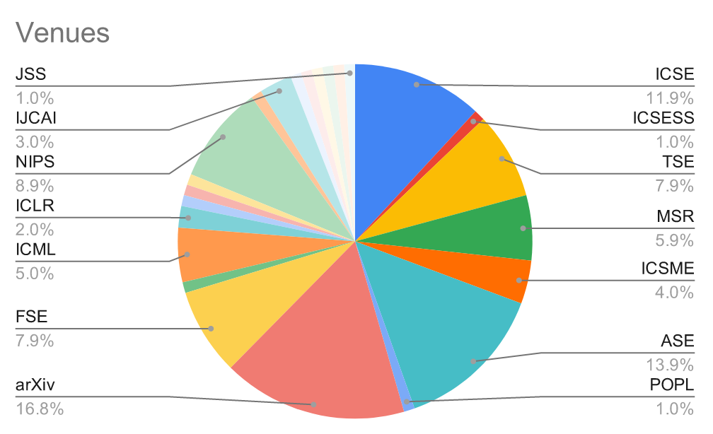
Figure 2. The distribution of papers across venues

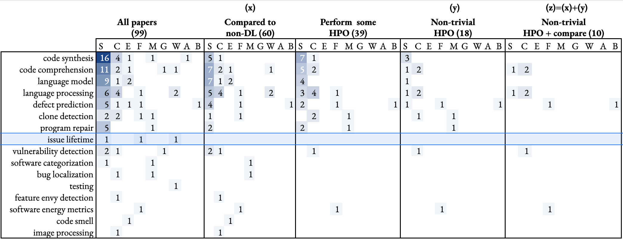
Figure 3. A summary of our literature review of deep learning methods in SE. The blue row denotes the DeepTriage system used in this paper. Legend: A = attention mechanism, B = deep belief network, C = convolutional networks, E = embedding, F = feedforward networks (which includes traditional perceptrons (Rosenblatt, 1961) (McCulloch and Pitts, 1943)) G = graph networks, M = misc (i.e. some particular architecture invented by the author, used in one paper), S = sequence, W = word2vec. For a list of the papers shown in the right-hand-side column, see Table 7.

7. Literature Review: deep learning in SE

Using a literature review, this section argues that the issue raised in this paper (that researchers seen rush to use the latest methods from deep learning literature, without baselining them against simpler) is widespread in the software analytics literature.

To understand how deep learning are used in SE, we performed the following steps.

• Seed: Our approach started with collecting relevant papers. As a seed, we collected papers from the recent literature review conducted by Watson  (Watson, 2020).

• Search: To this list, we added papers added by our own searches on Google Scholar. Our search keywords included “deep learning AND software”, “deep learning AND defect prediction”, and “deep learning AND bug fix” (this last criteria was added since we found that some recent papers, such as Lee et al (2020), used the term “bug fix time” rather than “issue close time”).

• Filter: Next, we filtered papers using the following criteria: (a) published in top venues as listed in Google Scholar metrics for Software Systems, Artificial Intelligence, and Computational Linguistics; or, released on arXiv in the last 3 years or widely cited ($>$ 100 cites) (b) has at least 10 cites per year, unless it was published in or after 2017 (the last three years). The distribution of papers across different venues is shown in Figure 2.

• Backward Snowballing: As recommended by Wohlin (2014), we performed “snowballing” on our paper (i.e. we added papers cited by the papers in our list that also satisfy the criteria above). Our snowballing stopped when either (a) the list of papers cited by the current generation is a subset of the papers already in the list, or (b) there were no further papers found.

This led to a list of 99 papers, which we summarize in Figure 3. Some engineering judgement was used in assigning papers to the categories of that figure. For example, a paper on learning a latent embedding of an API  (Nguyen et al, 2017) for various purposes, such as discovering analogous APIs among third-parties  (Chen et al, 2019), was categorized as “code comprehension”. Similarly, most papers performing some variant of code translation, including API translation as in  (Gu et al, 2017), were categorized into “language processing”–a bin that contains programming language processing and natural language processing. Tasks that we could not justifiably merge into an existing bin (e.g. on image processing  (Ott et al, 2018; Sun et al, 2018) were given their own special category.

Note the numbers on top of the columns of Figure 3:

• Sightly more than half (60.1%) of those papers compare their results to non-DL methods. We suggest that number should be higher–it is important to benchmark new methods against prior state-of-the-art.

• Only a minority of papers (39.4%) performed any sort of hyper-parameter optimization (HPO), i.e., used methods that tune the various “hyper-parameters”, such as the number of layers of the deep learner, to eke out the best performance of deep learning (39.4%).

• Even fewer papers (18.2%) applied hyper-parameter optimization in a non-trivial manner; i.e., not using deprecated grid search (Bergstra and Bengio, 2012) and using a hold-out set to assess the tuning before going to a separate test set).

• Finally, few papers (10.1%) used both non-trivial hyper-parameter optimization and compared to results to prior non-deep learning work. These “best of breed” papers are listed in Table 7.

Table 7. Papers in Column (z) of Figure 3.

Paper	Reference
Suggesting Accurate Method and Class Names	(Allamanis et al, 2015)
Automated Vulnerability Detection in Source Code Using Deep Representation Learning	(Russell et al, 2018)
A convolutional attention network for extreme summarization of source code	(Allamanis et al, 2016)
Automating intention mining	(Huang et al, 2018)
Sentiment analysis for software engineering: How far can we go?	(Lin et al, 2018)
500+ times faster than deep learning: A case study exploring faster methods for text mining stackoverflow	(Menzies et al, 2018)
Automatically learning semantic features for defect prediction	(Wang et al, 2016)
Deep green: Modelling time-series of software energy consumption	(Romansky et al, 2017)
On the Value of Oversampling for Deep Learning in Software Defect Prediction	(Yedida and Menzies, 2021)

In summary, we find that the general pattern in the literature is that while there is much new work on deep learning, there is not so much work on comparing these new methods to older, simpler approaches. This is a concern since, as shown in this paper, those older simpler methods, being faster, are more amenable to hyper-parameter optimization, and can yield better results when tuned. As we stated above, 40% of papers do not compare against simpler, non-deep learning methods, and only 18% of papers apply hyper-parameter optimization to their approach, possibly due to the computational infeasible nature of doing so with more complex methods.

8. Discussion and Conclusion

In this paper, we explored the state of literature applying deep learning techniques to software engineering tasks. We discussed and explored a systemic tendency to choose fundamentally more complex models than needed. We used this, and the study by Galke and Scherp (2021) as motivation to apply simpler deep learning models to two software engineering tasks, predicting issue close time, and vulnerability detection. Our model is much simpler than prior state-of-the-art deep learning models and takes significantly less time to run. We argue that these “old but gold” models are sorely lacking in modern deep learning applied in SE, with researchers preferring to use more sophisticated methods.

As to why it performs so well, we hypothesize that the power of SIMPLE came from tuning the hyper-parameters. To test this, we also ran a feedforward architecture without tuning (see FF in Table 5). We note a stark difference between the performance of the untuned and tuned versions of this architecture.

From our results, we say that deep learning is a promising method, but should be considered in the context of other techniques. We suggest to the community that before analysts jump to more complex approaches, they try a simpler approach; at the very least, this will form a baseline that can endorse the value of the more complex learner. There is much literature on baselines in SE: for example, in his textbook on empirical methods for AI, Cohen (1995) strongly advocates comparing against simpler baselines. In the machine learning community, Holte (1993) uses the “OneR” baseline to judge the complexity of upcoming tasks. In the SE community, Whigham et al (2015) recently proposed baseline methods for effort estimation (for other baseline methods, see Mittas and Angelis (2012)). Shepperd and MacDonell (2012) argue convincingly that measurements are best viewed as ratios compared to measurements taken from some minimal baseline system. Work on cross versus within-company cost estimation has also recommended the use of some very simple baseline (they recommend regression as their default model (Kitchenham et al, 2006)).

Our results present a cautionary tale about the pitfalls of using deep learners. While it is certainly tempting to use the state-of-the-art results from deep learning literature (which, as prior work has shown, certainly yields good results), we advise the reader to instead attempt the use of simpler models and apply hyper-parameter tuning to achieve better performance, faster.

It is left as future work to explore whether this same principle of using SIMPLE models for other software engineering tasks works equally well. By relying on simple architectures of deep learners, we obtain faster, simpler, and more space-efficient models. This exploration naturally lends itself to the application of modern deep learning theory to further simplify these SIMPLE models. In particular, Han et al (2015) explored model compression techniques based on reduced-precision weights, an idea that is gaining increasing attention in the deep learning community (we refer the reader to  Gupta et al (2015) and  Wang et al (2018) for details, and  Tung and Mori (2018) for a parallel implementation of these techniques). Further, knowledge distillation  (Hinton et al, 2015), a method of training student learners (such as decision trees) from a parent deep learning model, has shown great promise, with the student learners outperforming the deep learners they were derived from. This would make it possible to have the accuracy of deep learning with the speed of decision tree learning.

To repeat some comments from the introduction, the experiments of this paper are based on two case studies. Hence, they do not show that all deep learners can be replaced by faster and simpler methods. That said, we would say that there is enough evidence here to give the software analytics reasons to pause, and reflect, on the merits of rushing headlong into new things without a careful consideration of all that has gone before.

Declarations

• Funding: None.

• Conflicts of interest/Competing interests: None.

• Availability of data and material: All data used in this manuscript is publicly available at https://github.com/mkris0714/Bug-Related-Activity-Logs.

• Code availability: All source code used is available at https://github.com/fastidiouschipmunk/simple.

References

- Aggarwal et al (2001) Aggarwal CC, Hinneburg A, Keim DA (2001) On the surprising behavior of distance metrics in high dimensional space. In: International conference on database theory, Springer, pp 420–434
- Agrawal and Menzies (2018) Agrawal A, Menzies T (2018) Is” better data” better than” better data miners”? In: 2018 IEEE/ACM 40th International Conference on Software Engineering (ICSE), IEEE, pp 1050–1061
- Agrawal et al (2019) Agrawal A, Fu W, Chen D, Shen X, Menzies T (2019) How to” dodge” complex software analytics. IEEE Transactions on Software Engineering
- Agrawal et al (2021) Agrawal A, Yang X, Agrawal R, Shen X, Menzies T (2021) Simpler hyperparameter optimization for software analytics: Why, how, when? arXiv preprint arXiv:200807334
- Akbarinasaji et al (2018) Akbarinasaji S, Caglayan B, Bener A (2018) Predicting bug-fixing time: A replication study using an open source software project. journal of Systems and Software 136:173–186
- Allamanis et al (2015) Allamanis M, Barr ET, Bird C, Sutton C (2015) Suggesting accurate method and class names. In: Proceedings of the 2015 10th Joint Meeting on Foundations of Software Engineering, pp 38–49
- Allamanis et al (2016) Allamanis M, Peng H, Sutton C (2016) A convolutional attention network for extreme summarization of source code. In: International conference on machine learning, pp 2091–2100
- Alon et al (2019) Alon U, Zilberstein M, Levy O, Yahav E (2019) code2vec: Learning distributed representations of code. Proceedings of the ACM on Programming Languages 3(POPL):1–29
- Badrinarayanan et al (2017) Badrinarayanan V, Kendall A, Cipolla R (2017) Segnet: A deep convolutional encoder-decoder architecture for image segmentation. IEEE transactions on pattern analysis and machine intelligence 39(12):2481–2495
- Bahdanau et al (2014) Bahdanau D, Cho K, Bengio Y (2014) Neural machine translation by jointly learning to align and translate. arXiv preprint arXiv:14090473
- Bergstra and Bengio (2012) Bergstra J, Bengio Y (2012) Random search for hyper-parameter optimization. The Journal of Machine Learning Research 13(1):281–305
- Bergstra et al (2011) Bergstra J, Bardenet R, Bengio Y, Kégl B (2011) Algorithms for hyper-parameter optimization. Advances in neural information processing systems 24:2546–2554
- Brown et al (2020) Brown TB, Mann B, Ryder N, Subbiah M, Kaplan J, Dhariwal P, Neelakantan A, Shyam P, Sastry G, Askell A, et al (2020) Language models are few-shot learners. arXiv preprint arXiv:200514165
- Chen et al (2019) Chen C, Xing Z, Liu Y, Ong KLX (2019) Mining likely analogical apis across third-party libraries via large-scale unsupervised api semantics embedding. IEEE Transactions on Software Engineering
- Chen and Zhou (2018) Chen Q, Zhou M (2018) A neural framework for retrieval and summarization of source code. In: Proceedings of the 33rd ACM/IEEE International Conference on Automated Software Engineering, Association for Computing Machinery, New York, NY, USA, ASE 2018, p 826–831, DOI 10.1145/3238147.3240471, URL https://doi.org/10.1145/3238147.3240471
- Cohen (1995) Cohen PR (1995) Empirical methods for artificial intelligence, vol 139. MIT press Cambridge, MA
- Fu et al (2016) Fu W, Menzies T, Shen X (2016) Tuning for software analytics: Is it really necessary? Information and Software Technology 76:135–146
- Galke and Scherp (2021) Galke L, Scherp A (2021) Forget me not: A gentle reminder to mind the simple multi-layer perceptron baseline for text classification. arXiv preprint arXiv:210903777
- Gao et al (2020) Gao Z, Jiang L, Xia X, Lo D, Grundy J (2020) Checking smart contracts with structural code embedding. IEEE Transactions on Software Engineering
- Giger et al (2010) Giger E, Pinzger M, Gall H (2010) Predicting the fix time of bugs. In: Proceedings of the 2nd International Workshop on Recommendation Systems for Software Engineering, pp 52–56
- Goodfellow et al (2016) Goodfellow I, Bengio Y, Courville A, Bengio Y (2016) Deep learning, vol 1. MIT press Cambridge
- Grieco et al (2016) Grieco G, Grinblat GL, Uzal L, Rawat S, Feist J, Mounier L (2016) Toward large-scale vulnerability discovery using machine learning. In: Proceedings of the Sixth ACM Conference on Data and Application Security and Privacy, pp 85–96
- Gu et al (2017) Gu X, Zhang H, Zhang D, Kim S (2017) Deepam: Migrate apis with multi-modal sequence to sequence learning. arXiv preprint arXiv:170407734
- Guo et al (2010) Guo PJ, Zimmermann T, Nagappan N, Murphy B (2010) Characterizing and predicting which bugs get fixed: an empirical study of microsoft windows. In: Proceedings of the 32Nd ACM/IEEE International Conference on Software Engineering-Volume 1, pp 495–504
- Gupta et al (2015) Gupta S, Agrawal A, Gopalakrishnan K, Narayanan P (2015) Deep learning with limited numerical precision. In: International Conference on Machine Learning, pp 1737–1746
- Habayeb et al (2017) Habayeb M, Murtaza SS, Miranskyy A, Bener AB (2017) On the use of hidden markov model to predict the time to fix bugs. IEEE Transactions on Software Engineering 44(12):1224–1244
- Han et al (2015) Han S, Mao H, Dally WJ (2015) Deep compression: Compressing deep neural networks with pruning, trained quantization and huffman coding. arXiv preprint arXiv:151000149
- Hinton et al (2015) Hinton G, Vinyals O, Dean J (2015) Distilling the knowledge in a neural network. arXiv preprint arXiv:150302531
- Hoang et al (2019) Hoang T, Dam HK, Kamei Y, Lo D, Ubayashi N (2019) Deepjit: an end-to-end deep learning framework for just-in-time defect prediction. In: 2019 IEEE/ACM 16th International Conference on Mining Software Repositories (MSR), IEEE, pp 34–45
- Hochreiter and Schmidhuber (1997) Hochreiter S, Schmidhuber J (1997) Long short-term memory. Neural computation 9(8):1735–1780
- Holte (1993) Holte RC (1993) Very simple classification rules perform well on most commonly used datasets. Machine learning 11(1):63–90
- Huang et al (2018) Huang Q, Xia X, Lo D, Murphy GC (2018) Automating intention mining. IEEE Transactions on Software Engineering
- Jiang and Agrawal (2018) Jiang P, Agrawal G (2018) A linear speedup analysis of distributed deep learning with sparse and quantized communication. In: Proceedings of the 32nd International Conference on Neural Information Processing Systems, pp 2530–2541
- John (1992) John H (1992) Genetic algorithms. Scientific american 267(1):44–50
- Kikas et al (2016) Kikas R, Dumas M, Pfahl D (2016) Using dynamic and contextual features to predict issue lifetime in github projects. In: Proceedings of the 13th International Conference on Mining Software Repositories, Association for Computing Machinery, New York, NY, USA, MSR ’16, p 291–302, DOI 10.1145/2901739.2901751, URL https://doi.org/10.1145/2901739.2901751
- Kim et al (2017) Kim S, Woo S, Lee H, Oh H (2017) Vuddy: A scalable approach for vulnerable code clone discovery. In: 2017 IEEE Symposium on Security and Privacy (SP), IEEE, pp 595–614
- Kingma and Ba (2014) Kingma DP, Ba J (2014) Adam: A method for stochastic optimization. arXiv preprint arXiv:14126980
- Kipf and Welling (2016) Kipf TN, Welling M (2016) Semi-supervised classification with graph convolutional networks. arXiv preprint arXiv:160902907
- Kitchenham et al (2006) Kitchenham B, Mendes E, Travassos GH (2006) A systematic review of cross-vs. within-company cost estimation studies. In: 10th International Conference on Evaluation and Assessment in Software Engineering (EASE) 10, pp 1–10
- Le et al (2011) Le QV, Ngiam J, Coates A, Lahiri A, Prochnow B, Ng AY (2011) On optimization methods for deep learning. In: ICML
- LeCun et al (2015) LeCun Y, Bengio Y, Hinton G (2015) Deep learning. nature 521(7553):436–444
- Lee et al (2020) Lee Y, Lee S, Lee C, Yeom I, Woo H (2020) Continual prediction of bug-fix time using deep learning-based activity stream embedding. IEEE Access 8:10503–10515
- Lee et al (2020) Lee Y, Lee S, Lee CG, Yeom I, Woo H (2020) Continual prediction of bug-fix time using deep learning-based activity stream embedding. IEEE Access 8:10503–10515
- Levina and Bickel (2004) Levina E, Bickel P (2004) Maximum likelihood estimation of intrinsic dimension. Advances in neural information processing systems 17:777–784
- Li et al (2018a) Li H, Xu Z, Taylor G, Studer C, Goldstein T (2018a) Visualizing the loss landscape of neural nets. In: Advances in Neural Information Processing Systems, pp 6389–6399
- Li et al (2018b) Li Z, Zou D, Xu S, Ou X, Jin H, Wang S, Deng Z, Zhong Y (2018b) Vuldeepecker: A deep learning-based system for vulnerability detection. arXiv preprint arXiv:180101681
- Lin et al (2018) Lin B, Zampetti F, Bavota G, Di Penta M, Lanza M, Oliveto R (2018) Sentiment analysis for software engineering: How far can we go? In: Proceedings of the 40th International Conference on Software Engineering, pp 94–104
- Liu et al (2019) Liu H, Jin J, Xu Z, Bu Y, Zou Y, Zhang L (2019) Deep learning based code smell detection. IEEE Transactions on Software Engineering
- Mani et al (2019) Mani S, Sankaran A, Aralikatte R (2019) Deeptriage: Exploring the effectiveness of deep learning for bug triaging. In: COMAD’19: ACM India Joint International Conference on Data Science and Management of Data, pp 171–179
- Marks et al (2011) Marks L, Zou Y, Hassan AE (2011) Studying the fix-time for bugs in large open source projects. In: Proceedings of the 7th International Conference on Predictive Models in Software Engineering, pp 1–8
- Martens et al (2010) Martens J, et al (2010) Deep learning via hessian-free optimization. In: ICML, vol 27, pp 735–742
- McCulloch and Pitts (1943) McCulloch WS, Pitts W (1943) A logical calculus of the ideas immanent in nervous activity. The bulletin of mathematical biophysics 5(4):115–133
- Menzies et al (2018) Menzies T, Majumder S, Balaji N, Brey K, Fu W (2018) 500+ times faster than deep learning:(a case study exploring faster methods for text mining stackoverflow). In: 2018 IEEE/ACM 15th International Conference on Mining Software Repositories (MSR), IEEE, pp 554–563
- Mikolov et al (2013a) Mikolov T, Chen K, Corrado G, Dean J (2013a) Efficient estimation of word representations in vector space. arXiv preprint arXiv:13013781
- Mikolov et al (2013b) Mikolov T, Sutskever I, Chen K, Corrado GS, Dean J (2013b) Distributed representations of words and phrases and their compositionality. In: Advances in neural information processing systems, pp 3111–3119
- Mittas and Angelis (2012) Mittas N, Angelis L (2012) Ranking and clustering software cost estimation models through a multiple comparisons algorithm. IEEE Transactions on software engineering 39(4):537–551
- Montufar et al (2014) Montufar GF, Pascanu R, Cho K, Bengio Y (2014) On the number of linear regions of deep neural networks. In: Advances in neural information processing systems, pp 2924–2932
- Nair and Hinton (2010) Nair V, Hinton GE (2010) Rectified linear units improve restricted boltzmann machines. In: ICML
- Nguyen et al (2017) Nguyen TD, Nguyen AT, Phan HD, Nguyen TN (2017) Exploring api embedding for api usages and applications. In: 2017 IEEE/ACM 39th International Conference on Software Engineering (ICSE), IEEE, pp 438–449
- Ott et al (2018) Ott J, Atchison A, Harnack P, Bergh A, Linstead E (2018) A deep learning approach to identifying source code in images and video. In: 2018 IEEE/ACM 15th International Conference on Mining Software Repositories (MSR), IEEE, pp 376–386
- Pearson (1901) Pearson K (1901) Liii. on lines and planes of closest fit to systems of points in space. The London, Edinburgh, and Dublin Philosophical Magazine and Journal of Science 2(11):559–572
- Rees-Jones et al (2017) Rees-Jones M, Martin M, Menzies T (2017) Better predictors for issue lifetime. arXiv preprint arXiv:170207735
- Romansky et al (2017) Romansky S, Borle NC, Chowdhury S, Hindle A, Greiner R (2017) Deep green: Modelling time-series of software energy consumption. In: 2017 IEEE International Conference on Software Maintenance and Evolution (ICSME), IEEE, pp 273–283
- Rosenblatt (1961) Rosenblatt F (1961) Principles of neurodynamics. perceptrons and the theory of brain mechanisms. Tech. rep., Cornell Aeronautical Lab Inc Buffalo NY
- Rosenthal et al (1994) Rosenthal R, Cooper H, Hedges L (1994) Parametric measures of effect size. The handbook of research synthesis 621(2)
- Rumelhart et al (1985) Rumelhart DE, Hinton GE, Williams RJ (1985) Learning internal representations by error propagation. Tech. rep., California Univ San Diego La Jolla Inst for Cognitive Science
- Russell et al (2018) Russell R, Kim L, Hamilton L, Lazovich T, Harer J, Ozdemir O, Ellingwood P, McConley M (2018) Automated vulnerability detection in source code using deep representation learning. In: 2018 17th IEEE international conference on machine learning and applications (ICMLA), IEEE, pp 757–762
- Shepperd and MacDonell (2012) Shepperd M, MacDonell S (2012) Evaluating prediction systems in software project estimation. Information and Software Technology 54(8):820–827
- Sun et al (2018) Sun SH, Noh H, Somasundaram S, Lim J (2018) Neural program synthesis from diverse demonstration videos. In: International Conference on Machine Learning, pp 4790–4799
- Tantithamthavorn et al (2016) Tantithamthavorn C, McIntosh S, Hassan AE, Matsumoto K (2016) Automated parameter optimization of classification techniques for defect prediction models. In: Proceedings of the 38th International Conference on Software Engineering, Association for Computing Machinery, New York, NY, USA, ICSE ’16, p 321–332, DOI 10.1145/2884781.2884857, URL https://doi.org/10.1145/2884781.2884857
- Thornton et al (2013) Thornton C, Hutter F, Hoos HH, Leyton-Brown K (2013) Auto-weka: Combined selection and hyperparameter optimization of classification algorithms. In: Proceedings of the 19th ACM SIGKDD international conference on Knowledge discovery and data mining, pp 847–855
- Tung and Mori (2018) Tung F, Mori G (2018) Clip-q: Deep network compression learning by in-parallel pruning-quantization. In: Proceedings of the IEEE Conference on Computer Vision and Pattern Recognition, pp 7873–7882
- Vaswani et al (2017) Vaswani A, Shazeer N, Parmar N, Uszkoreit J, Jones L, Gomez AN, Kaiser Ł, Polosukhin I (2017) Attention is all you need. In: Advances in neural information processing systems, pp 5998–6008
- Viega et al (2000) Viega J, Bloch JT, Kohno Y, McGraw G (2000) Its4: A static vulnerability scanner for c and c++ code. In: Proceedings 16th Annual Computer Security Applications Conference (ACSAC’00), IEEE, pp 257–267
- Vieira et al (2019) Vieira R, da Silva A, Rocha L, Gomes JP (2019) From reports to bug-fix commits: A 10 years dataset of bug-fixing activity from 55 apache’s open source projects. In: Proceedings of the Fifteenth International Conference on Predictive Models and Data Analytics in Software Engineering, pp 80–89
- Wang et al (2018) Wang N, Choi J, Brand D, Chen CY, Gopalakrishnan K (2018) Training deep neural networks with 8-bit floating point numbers. In: Advances in neural information processing systems, pp 7675–7684
- Wang et al (2016) Wang S, Liu T, Tan L (2016) Automatically learning semantic features for defect prediction. In: 2016 IEEE/ACM 38th International Conference on Software Engineering (ICSE), IEEE, pp 297–308
- Watson (2020) Watson CA (2020) Deep learning in software engineering. PhD thesis, College of William & Mary
- Weiss et al (2007) Weiss C, Premraj R, Zimmermann T, Zeller A (2007) How long will it take to fix this bug? In: Fourth International Workshop on Mining Software Repositories (MSR’07: ICSE Workshops 2007), IEEE, pp 1–1
- Whigham et al (2015) Whigham PA, Owen CA, Macdonell SG (2015) A baseline model for software effort estimation. ACM Transactions on Software Engineering and Methodology (TOSEM) 24(3):1–11
- Wohlin (2014) Wohlin C (2014) Guidelines for snowballing in systematic literature studies and a replication in software engineering. In: Proceedings of the 18th international conference on evaluation and assessment in software engineering, pp 1–10
- Yamaguchi et al (2014) Yamaguchi F, Golde N, Arp D, Rieck K (2014) Modeling and discovering vulnerabilities with code property graphs. In: 2014 IEEE Symposium on Security and Privacy, IEEE, pp 590–604
- Yedida and Menzies (2021) Yedida R, Menzies T (2021) On the value of oversampling for deep learning in software defect prediction. IEEE Transactions on Software Engineering
- Zhou et al (2019) Zhou Y, Liu S, Siow J, Du X, Liu Y (2019) Devign: Effective vulnerability identification by learning comprehensive program semantics via graph neural networks. In: Advances in Neural Information Processing Systems, pp 10197–10207