Automated Diagnosis of Intestinal Parasites: A new hybrid approach and its benefits

Abstract

Intestinal parasites are responsible for several diseases in human beings. In order to eliminate the error-prone visual analysis of optical microscopy slides, we have investigated automated, fast, and low-cost systems for the diagnosis of human intestinal parasites. In this work, we present a hybrid approach that combines the opinion of two decision-making systems with complementary properties: ($DS_{1}$) a simpler system based on very fast handcrafted image feature extraction and support vector machine classification and ($DS_{2}$) a more complex system based on a deep neural network, Vgg-16, for image feature extraction and classification. $DS_{1}$ is much faster than $DS_{2}$, but it is less accurate than $DS_{2}$. Fortunately, the errors of $DS_{1}$ are not the same of $DS_{2}$. During training, we use a validation set to learn the probabilities of misclassification by $DS_{1}$ on each class based on its confidence values. When $DS_{1}$ quickly classifies all images from a microscopy slide, the method selects a number of images with higher chances of misclassification for characterization and reclassification by $DS_{2}$. Our hybrid system can improve the overall effectiveness without compromising efficiency, being suitable for the clinical routine — a strategy that might be suitable for other real applications. As demonstrated on large datasets, the proposed system can achieve, on average, 94.9%, 87.8%, and 92.5% of Cohen’s Kappa on helminth eggs, helminth larvae, and protozoa cysts, respectively.

Keywords— Image classification,Microscopy image analysis, Automated diagnosis of intestinal parasites, Support vector machines, Deep neural networks

1 Introduction

A recent report by the World Health Organization indicates that approximately 1.5 billion people are infected with intestinal parasites [1]. These parasitic diseases are most common in tropical countries due to climate, precarious health services, poor sanitary conditions, among several other factors. The problem can cause mental and physical disorders (e.g., the difficulty of concentration, diarrhea, abdominal pain) or, in the extreme case, death, especially in infants and immunodeficient individuals.

The diagnostic procedure of the causative agent for parasitic infections still relies on the visual analysis of optical microscopy slides — an error-prone procedure that usually results in low to moderate diagnostic sensitivity [2]. In order to circumvent the problem, we have developed the first automated system for the diagnosis (the DAPI system) of the 15 most common species of human intestinal parasites in Brazil [3, 4]. Examples are presented in Figures 1 and 2.

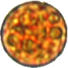
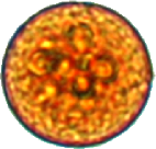
(a)	(b)	(c)	(d)	(e)	(f)

Figure 1: Examples of protozoan. (a) Entamoeba histolytica/E. dispar; (b) Giardia duodenalis; (c) Entamoeba coli; (d) Endolimax nana; (e) Iodamoeba bütschlii; (f) Blastocystis hominis.

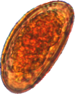
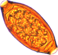
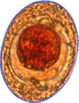
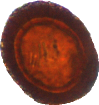
(a)	(b)	(c)	(d)
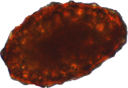
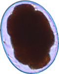
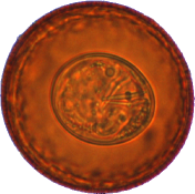
(e) (f) (g)
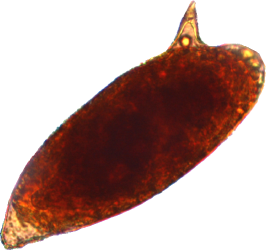
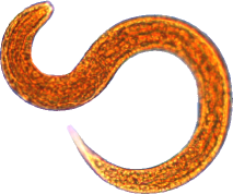
(h) (i)

Figure 2: Examples of helminths: (a) Enterobius vermicularis; (b) Trichuris trichiura; (c) Hymenolepis nana; (d) Taenia spp.; (e) Ascaris lumbricoides; (f) Ancylostomatidae; (g) Hymenolepis diminuta; (h) Schistosoma mansoni; (i) Strongyloides stercoralis larvae.

The DAPI system can produce about 2,000 images per microscopy slide, with 4M pixels each and 12 bits per color channel. These images are acquired on a compromise focus plane  and processed in less than 4 minutes on a modern PC (Core i7 CPU with 16 threads) — a time acceptable for the clinical routine. Our system can successfully segment objects (parasites and similar impurities), separate them into three groups, and align them for feature extraction and classification. These groups are: (a) helminth eggs, (b) protozoa cysts and vacuolar form of protozoa (Blastocystis hominis), and (c) helminth larvae, all of them with similar fecal impurities which are not eliminated during object segmentation.

The main question we seek to answer here is: can we benefit from the higher effectiveness of deep neural networks without compromising the efficiency and cost of the DAPI system? Although machines have become faster, digital cameras can also generate higher resolution images, and the DAPI system can also improve and produce more images from multiple microscopy slides and with different focus depth. Therefore, we believe that it will be always desirable to improve effectiveness without compromising the efficiency and cost of image analysis systems. Such a constraint is crucial to make the DAPI system viable for the public health system.

In this work, we present a hybrid approach that combines the opinion of two decision-making systems with complementary properties and validate it for the diagnosis of those 15 most common species of human intestinal parasites in Brazil. The first system ($DS_{1}$) is based on very fast handcrafted image feature extraction [4] and support vector machine (the probabilistic $p$-SVM [5]) classification. The time to extract those handcrafted features is negligible and the $p$-SVM classifier takes time equivalent to a decision layer of a deep neural network since both can benefit from parallel matrix multiplication. As we demonstrate in our experiments, among several SVM and deep neural network models, we found $p$-SVM and Vgg-16 [6] the best options for $DS_{1}$ and $DS_{2}$, respectively. Vgg-16 uses 15 extra neuronal layers with a total number of neurons much higher than its decision layer, which makes $DS_{1}$ about 30 times faster than $DS_{2}$ when using a same GPU board (GeForce GTX 1060 6GB/PCIe/SSE2). On the other hand, $DS_{2}$ can be considerably more accurate than $DS_{1}$. Fortunately, the errors of $DS_{1}$ and $DS_{2}$ are not the same, given that they are statistically independent.

We then propose a hybrid approach that relies on a validation set to learn the probabilities of misclassification by $DS_{1}$ on each class based on its confidence values. Note that, as we will show, the confidence values of $p$-SVM are not inversely proportional to its chances of error. When $DS_{1}$ quickly classifies all images from a microscopy slide, the method selects the images with higher chances to have been misclassified by $DS_{1}$ and allows those images to be characterized and reclassified by $DS_{2}$. By that, our method can improve the overall effectiveness of the DAPI system without compromising its efficiency and cost — a strategy that can be used in other real applications involving image analysis. Our experiments demonstrate this result for large datasets by first comparing $DS_{1}$, $DS_{2}$, and our hybrid approach. We then show a comparison among several deep neural networks, that justifies our choice for Vgg-16, and comparison among SVM models and the previous Optimum-Path Forest classifier used in [4], that justifies our choice for $p$-SVM.

The remaining sections are organized as follows. Section 2 presents the related works on image classification of intestinal parasites and our previous version of the automated system for the diagnosis of intestinal parasites. Sections 3 and 4 present the materials and the proposed hybrid approach based on $DS_{1}$ and $DS_{2}$. The experimental results with discussion and the conclusions are presented in Sections 5 and 6, respectively.

2 Related works

In Computer Vision, several works have presented methods to process and classify images of parasites from different means (e.g., blood, intestine, water, and skin). Most works rely on classical image processing and machine learning techniques [7, 8, 9, 10, 11, 3, 12]. Recent efforts have also been made towards the automated diagnosis of human intestinal parasites [13, 14, 15, 16]. However, it is difficult to compare them with our work. They do not usually mention the parasitological protocol adopted to create the microscopy slides, which is crucial to make the automated image analysis feasible — e.g., a considerable reduction in fecal impurities may facilitate the image analysis, but at the cost of losing some species of parasites in the microscopy slide. The DAPI system is a complete solution, from the collection, storage, transportation, and processing of fecal samples to create microscopy slides for automated image acquisition and analysis using a compromise focus plane. In those works, fecal impurities are not usually present and the images are acquired with manual focus. We then compare the methods in this paper with 13 deep neural networks and previous works [3, 4, 17], all based on the DAPI system.

The DAPI system [3] is composed of one optical microscope with a motorized stage, focus driver, and digital camera, all controlled by a computer. In [4], one can find improvements and details about the image processing and machine learning techniques adopted to find a common focus plane for image acquisition, to segment objects (parasites and similar impurities) from the images, to align the objects based on principal component analysis, to characterize each object based on handcrafted (texture, color, and shape) features, and to classify them into one out of 16 classes (15 species of parasites and fecal impurity). In this work, we will use the same preprocessing operations that separate the segmented objects into three groups: (i) helminth eggs, (ii) protozoa cysts and vacuolar form of protozoa, and (iii) helminth larvae, each with their similar fecal impurities, for subsequent characterization and classification. Figure 3 illustrates how similar can be these impurity objects to the real parasites and Figure 4 shows that even examples of the same class might be different among them, due to different living stages of the parasite.

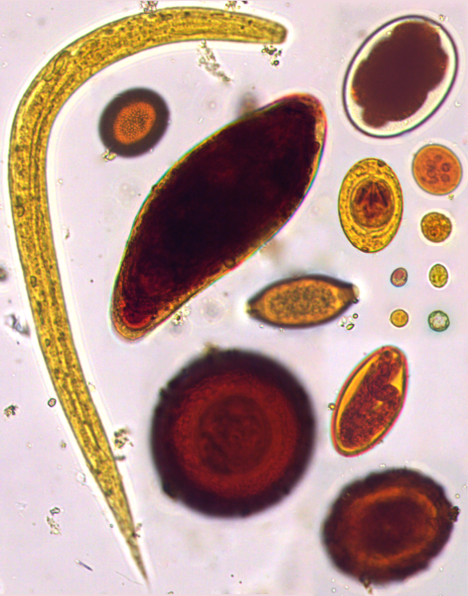
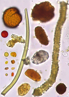
(a)	(b)

Figure 3: (a) The 15 most common species of human intestinal parasites in Brazil and (b) similar impurity objects  [17].

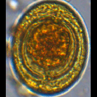
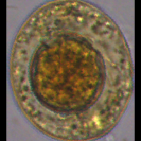
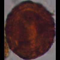
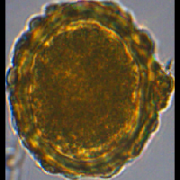
(a)	(b)	(c)	(d)
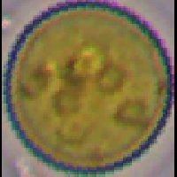
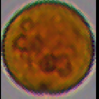
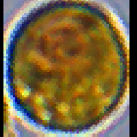
(e)	(f)	(g)	(h)

Figure 4: Intra-class differences. (a-b) Hymenolepis nana, (c-d) Ascaris lumbricoides, (e-f) Entamoeba coli, and (g-h) Iodamoeba bütschlii.

Our preliminary works used a dataset with less than 8,000 images while the present work uses a dataset with almost 52,000 images. A higher number of images called our attention to the importance of using more effective characterization and classification techniques — a pair of operations that we call a decision system. In [3], for instance, the experiments showed that the Optimum-Path Forest (OPF) classifier [18] was the best choice for classification. In this work, we show that $p$-SVM is a better choice than OPF for our first decision system, $DS_{1}$.

In the meantime, we have investigated parasitological techniques to create microscopy slides richer in parasites and with less impurities [2] (see Figure 5), and we have also observed on a dataset with 16,437 images that convolutional neural networks can considerably improve characterization and classification of human intestinal parasites [17]. Given that, we decided to further investigate deep neural networks and came to the current proposal of combining $DS_{1}$ with a decision system $DS_{2}$ based on Vgg-16.

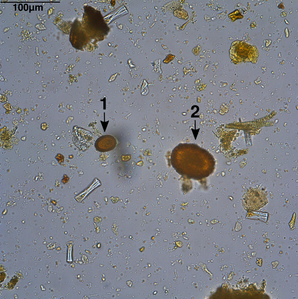
Figure 5: The input for object segmentation: field image from a microscopy slide showing a Taenia spp. egg (Arrow 1) and an A. lumbricoides fertile egg (Arrow 2).

3 Materials

In this section, we describe the datasets used for the experiments, which contain a total of 51,919 images with the 15 most common species of human intestinal parasites in Brazil and similar fecal impurities. Stool samples have been obtained from the regions of Campinas and Araçatuba, São Paulo, Brazil, and processed in our lab (Laboratory of Image Data Science/LIDS) in Campinas, São Paulo, Brazil by using a parasitological technique called TF-Test Modified [2] — a technique based on the centrifugation-sedimentation principle to concentrate parasites and reduce the amount of fecal impurities in optical microscopy slides. After parasitological processing, microscopy slides were prepared and used in our system for automated image acquisition. The objects in those images were automatically segmented, aligned, and separated into three groups [4], being the class of each one identified by experts in Parasitology (or confirmed by the experts after their automated recognition in our system). These groups and classes are as follows.

1. Helminth eggs: H. nana, H. diminuta, Ancylostomatidae , E. vermicularis, A. lumbricoides, T. trichiura, S. mansoni, Taenia spp. and impurities of similar size and shape, named EGG-9;

2. Cysts and vacuolar form of protozoa: E. coli, E. histolytica / E. dispar, E. nana, Giardia, I. bütschlii, B. hominis and impurities of similar size and shape, named PRO-7;

3. Helminth larvae: S. stercoralis and impurities with similar size and shape, named LAR-2;

Table 1 presents the number of images in our database per group and class in each group. One can notice that each group represents one seriously unbalanced dataset with considerably more fecal impurities than parasites. Indeed, this reflects what is likely found in regular exams. Given that unbalanced datasets can critically affect the performance of classification systems and the impurities are numerous with similar examples to any other category, this can be considered a challenging problem.

Parasites Database
Database Groups	Number	Category	Class ID
LAR-2	501	Strongyloides stercoralis	1
	1351	Impurities	2
	1852	Total
EGG-9	501	Hymenolepis nana	1
	83	Hymenolepis diminuta	2
	286	Ancylostomatidae	3
	103	Enterobius vermicularis	4
	835	Ascaris lumbricoides	5
	435	Trichuris trichiura	6
	254	Schistosoma mansoni	7
	379	Taenia spp.	8
	9815	Impurities	9
	12691	Total
PRO-7	869	Entamoeba coli	1
	659	Entamoeba histolytica / E. dispar	2
	1783	Endolimax nana	3
	1931	Giardia duodenalis	4
	3297	Iodamoeba bütschlii	5
	309	Blastocystis hominis	6
	28528	Impurities	7
	37376	Total

Table 1: Most common species of human intestinal parasites in Brazil: number of images per group and category in each group.

The experiments use a PC with the following specifications: Intel (R) Core (TM) i7-7700 - 3.60 GHz (8 CPU), RAM - 64 GiB, LINUX operating system (Ubuntu - 16:04 LTS - 64 bit) and GeForce GTX 1060 6GB/PCIe/SSE2.

As we will see next, our methodology requires a validation set. Therefore, each group, EGG-9, PRO-7, and LAR-2, is divided into training, validation, and testing sets for the experiments (as described in Section 5) and this process is also repeated 10 times to obtain reliable statistical results.

4 Methods

Figure 6 shows a flow chart of the DAPI system. Fecal samples are collected, stored, transported by using the TF-Test kit and processed in our laboratory by using the TF-Test Modified protocol [2], creating an optical microscopy slide for automated image acquisition by following a single compromise plane of focus [3, 4]. Each slide generates about 2,000 images (e.g., Figure 5), which might be out of focus for some objects. Image segmentation involves a sequence of IFT-based image processing operations [19] suitable to separate parasites and impurities, in some situations that they appear connected, as illustrated in Figure 7. The segmentation mask is used for image alignment by principal component analysis — i.e., to align an image of a region of interest (ROI) around each object (Figure 4), which is used as input to the proposed hybrid decision system.

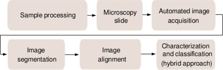
Figure 6: Data flow of the DAPI system.

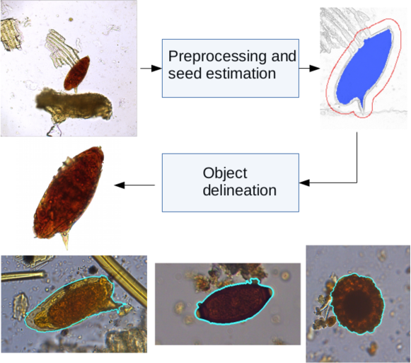
Figure 7: At the top, each slide field image is preprocessed by enhancing, automatic thresholding, IFT-based connected operators, and an area filter in order to estimate internal (blue) and external (red) seed pixels, as shown on a gradient image. Object delineation uses the IFT-watershed operator — seeds compete among themselves and the object is defined by the pixels conquered by minimum-cost paths from the internal seeds, where the cost of a path is the maximum gradient value along it. At the bottom, it shows three other examples of segmentation (cyan) in the presence of impurities: S. mansoni (left), T. trichiura (center), and A. lumbricoides (right).

For any group, EGG-9, PRO-7, or LAR-2, let $Z_{1}$, $Z_{2}$, and $Z_{3}$ be its corresponding training, validation, and testing sets, $Z_{1}\cap Z_{2}\cap Z_{3}=\emptyset$. Each image (after image segmentation and alignment) $s\in Z_{1}\cup Z_{2}\cup Z_{3}$ may come from one of $m$ classes $w_{j}$, $j=1,2,\ldots,m$. The proposed hybrid system relies on two decision-making systems with complementary properties:

• $DS_{1}$ is based on very fast handcrafted feature extraction [4] and $p$-SVM classification [5].

• $DS_{2}$ is based on Vgg-16 [6] for feature extraction and classification.

For characterization in $DS_{1}$, the method uses the aligned segmentation mask and combines the BIC color descriptor from [20] with the object area, perimeter, symmetry, major and minor axes of the best fit ellipse within the object, the difference between the ellipse and the object, energy, entropy, variance, and homogeneity of a co-occurrence matrix. These features are used with different weights in a single feature vector. The Multi-Scale Parameter Search algorithm (MSPS) [21] is applied to find the weight of each feature that maximizes classification accuracy in the training set. The final weights modify the Euclidean distance between the feature vectors of two objects during classification. In $DS_{2}$, characterization is obtained at the output of the last convolutional layer of Vgg-16 (similarly to any other CNN, before the layers of a MLP classifier) and its parameters are learned by backpropagation. Note that, $DS_{1}$ depends on the success of segmentation more than $DS_{2}$. For $DS_{2}$, segmentation only affects the alignment of the input ROI image.

While $DS_{1}$ is about 30 times faster than $DS_{2}$, the latter is considerably more accurate than the former. The main idea is that $DS_{1}$ should assign a class $w_{j}$, $j\in[1,m]$, to an image $s$, with a confidence value that $s$ comes from $w_{j}$. The hybrid method uses that confidence value to select the most likely misclassified images by $DS_{1}$ to be processed by $DS_{2}$. However, in order to improve effectiveness without compromising efficiency and cost, a limited number of images must be selected from the 2,000 images of a microscopy slide.

Let $c$ be a random variable that represents the confidence values assigned to images by $DS_{1}$. The probability of error $P_{error}(c\backslash w_{j})$, when $DS_{1}$ assigns an image $s$ to a class $w_{j}$ with confidence value $c$, should be inversely proportional to $c$, but we have observed that this is not usually the case with $p$-SVM. In order to circumvent the problem, we use a validation set to estimate probability distributions $P_{error}(c_{i}\backslash w_{j})$, $j=1,2,\ldots,m$, as normalized histograms with $n$ intervals (bins) $c_{i}$, $i=1,2,\ldots,n$. When $DS_{1}$ classifies the objects extracted from images of a microscopy slide, the object images with confidence values that fall in bins with higher probability of error $P_{error}(c_{i}\backslash w_{j})$ have higher priority to be selected for characterization and reclassification by $DS_{2}$.

The proposed training and testing phases of $DS_{1}$ and $DS_{2}$ for the hybrid method are described next.

4.1 Training our hybrid decision system

Figure 8a illustrates the training processes of $DS_{1}$ and $DS_{2}$ using images from $Z_{1}$. While Vgg-16 is trained by backpropagation from pre-aligned ROI images [6], $p$-SVM [5] is trained from the handcrafted features extracted from pre-segmented and aligned objects, as proposed in [4]. The implementation details about both training processes are given in Section 5.1.

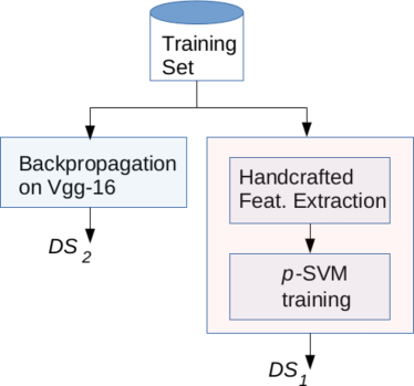
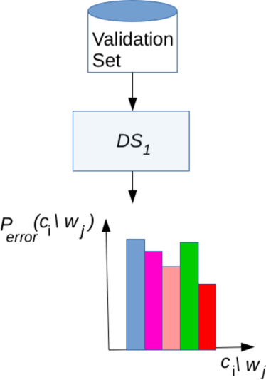
(a)	(b)

Figure 8: (a) Training of the decision systems $DS_{1}$ and $DS_{2}$. (b) After training, $DS_{1}$ is used on a validation set to estimate $P_{error}(c_{i}\backslash w_{j})$ for each class $w_{j}$, $j=1,2,\ldots,m$, and interval (bin) $c_{i}$, $i=1,2,\ldots,n$.

In Figure 8b, we estimate $P_{error}(c_{i}\backslash w_{j})$ by dividing the confidence values of $DS_{1}$ into $n>1$ intervals $c_{i}$ (bins), $i=1,2,\ldots,n$, and computing for each bin the percentage of images from a validation set $Z_{2}$ that are misclassified by $DS_{1}$ as belonging to each class $w_{j}$, $j=1,2,\ldots,m$. This results into $m$ histograms $P_{error}(c_{i}\backslash w_{j})$, as illustrated in Figure 9 for three classes and $n=20$ bins. Note that they are not inversely proportional to the confidence values for any class.

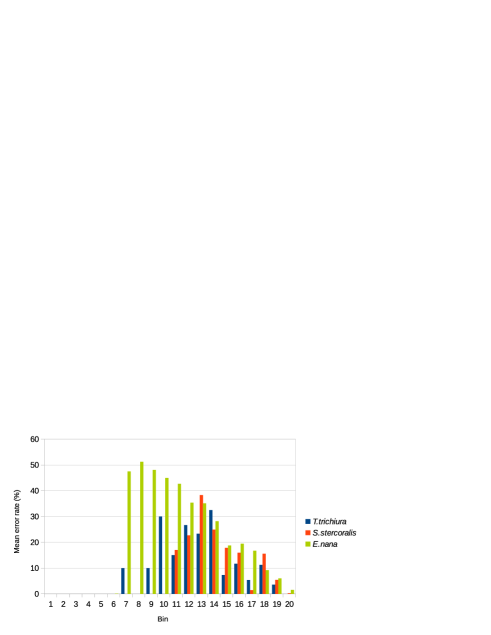
Figure 9: The histograms $P_{error}(c_{i}\backslash w_{j})$ for three classes of helminth eggs and $n=20$ bins.

4.2 Testing our hybrid decision system

A test set $Z_{3}$ contains objects that are segmented for image alignment and feature extraction. $DS_{1}$ is used to classify those objects in one of the classes $w_{j}$, $j\in[1,m]$, with a confidence value $c$ that falls in one of the bins $c_{i}$, $i\in[1,n]$. A selector sorts the images of those objects by their decreasing order of $P_{error}(c_{i}\backslash w_{j})$. For a given number $M$ of selected images for characterization and reclassification by $DS_{2}$, the selector randomly picks $M_{j}=M\times P_{error}(c_{i}\backslash w_{j})$ images per class $w_{j}$, $j=1,2,\ldots,m$, and bin $c_{i}$, $i=1,2,\ldots,n$, by following their decreasing order of $P_{error}(c_{i}\backslash w_{j})$, until the total number of selected images is $M$. The selected images might be reassigned to a class $w_{k}\neq w_{j}$, $k\in[1,m]$, by $DS_{2}$, otherwise $w_{j}$ is the assigned class (Figure 10).

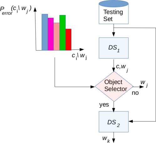
Figure 10: For each object in $Z_{3}$, $DS_{1}$ assigns a class $w_{j}$, $j\in[1,m]$, with confidence value $c$ that falls in a bin $c_{i}$, $i\in[1,n]$. Based on $P_{error}(c_{i}\backslash w_{j})$, the selector decides which object images will be processed by $DS_{2}$. It randomly picks images in their decreasing order of $P_{error}(c_{i}\backslash w_{j})$, until the total number of selected images is $M$. The selected images might be reassigned to a class $w_{k}\neq w_{j}$, $k\in[1,m]$, by $DS_{2}$, otherwise $w_{j}$ is the assigned class.

5 Experimental results and discussion

For the experiments, each dataset, EGG-9, PRO-7, and LAR-2, is divided into 40% for training ($Z_{1}$), 30% for validation ($Z_{2}$), and 30% for testing ($Z_{3}$) by using stratified random sampling. This process is also repeated 10 times to obtain reliable statistical results.

First, we evaluate the dependence of our approach with respect to the number $n$ of bins and select the best values for each group: $n=20$ bins for EGG-9 and $n=10$ bins for LAR-2 and PRO-7 (Section 5.1). We then show in the same section that our approach can be considerably more accurate than $DS_{1}$ and almost so accurate as $DS_{2}$ in most cases, being considerably faster than $DS_{2}$ and almost so fast as $DS_{1}$ . We also show that a random choice of object images for reclassification by $DS_{2}$ rather than a choice based on $P_{error}(c_{i}\backslash w_{j})$ is not a good option, which reinforces the importance of our approach. Second, we justify our choice for $p$-SVM in $DS_{1}$ by comparing different $SVM$ models and the OPF classifier in Section 5.2. Finally, we justify our choice for Vgg-16 in $DS_{2}$ by comparing it with several other deep neural networks in Section 5.3.

5.1 Hybrid approach versus $DS_{1}$ and $DS_{2}$

In $DS_{1}$, we optimize the parameters of $p$-SVM by using $Z1$ for training and $Z_{2}$ for evaluation, with parameter optimization based on grid search [22]. In $DS_{2}$, we started from Vgg-16 pre-trained on the Imagenet dataset and fine tuned it with the training set $Z_{1}$. For fine tuning, we fixed the learning rate at $1e^{-5}$, momentum at $0.9$, minibatch size at $16$, and the number of epochs at $150$. As recommended for neural networks pre-trained with the ImageNet dataset, the images were subtracted from the mean values of each band and interpolated to $224\times 224$ pixels and $3$ bands.

Given that the hybrid approach depends on the number $n$ of bins for $P_{error}(c_{i}\backslash w_{j})$, we first show its performance on $Z_{3}$ using Vgg-16 in $DS_{2}$ and $p$-SVM in $DS_{1}$ with $n$ equal to 10, 20, and 30 bins (Table 2). One can see that the best number of bins varies with the group: 10 bins for LAR-2 and PRO-7, and 20 bins for EGG-9. Therefore, these values are fixed for those groups in the next experiment.

Dataset	Technique	10 bins	20 bins	30 bins
EGG-9	proposed hybrid	0.947 $\pm$ 0.005	0.949 $\pm$ 0.007	0.948 $\pm$ 0.005
LAR-2	proposed hybrid	0.894 $\pm$ 0.020	0.878 $\pm$ 0.031	0.869 $\pm$ 0.020
PRO-7	proposed hybrid	0.926 $\pm$ 0.004	0.925 $\pm$ 0.004	0.925 $\pm$ 0.005

Table 2: Mean Cohen’s Kappa and the respective standard deviation over each group of parasites using $n$ equal to 10, 20 and 30 bins to build $P_{error}(c_{i}\backslash w_{j})$, $i\in[1,n]$ and $w_{j}\in[1,m]$.

Tables 3, 4, and 5 show the accuracy of each decision system on $Z_{3}$ in each group, EGG-9, LAR-2, and PRO-7, respectively. We have also added a variant of the hybrid system with random selection (RS) of object images for characterization and reclassification by $DS_{2}$. The hybrid approaches selected $M$ equal to 10% of the images in $Z_{3}$ for $DS_{2}$. This number was chosen to make the hybrid approaches acceptable for clinical routine (e.g., 4 minutes per microscopy slide in the current computer configuration).

Class	Technique
	$DS_{1}$	$DS_{2}$	Hybrid with RS	Prop. hybrid
H.nana	0.901 $\pm$ 0.020	0.995 $\pm$ 0.005	0.913 $\pm$ 0.016	0.987 $\pm$ 0.011
H.diminuta	0.736 $\pm$ 0.080	0.960 $\pm$ 0.018	0.780 $\pm$ 0.063	0.952 $\pm$ 0.025
Ancylostomatidae	0.915 $\pm$ 0.030	0.986 $\pm$ 0.012	0.921 $\pm$ 0.030	0.984 $\pm$ 0.014
E.vermicularis	0.742 $\pm$ 0.106	0.984 $\pm$ 0.022	0.758 $\pm$ 0.093	0.981 $\pm$ 0.022
A.lumbricoides	0.739 $\pm$ 0.043	0.970 $\pm$ 0.018	0.753 $\pm$ 0.036	0.960 $\pm$ 0.014
T.trichiura	0.902 $\pm$ 0.024	0.993 $\pm$ 0.007	0.909 $\pm$ 0.020	0.979 $\pm$ 0.007
S.mansoni	0.649 $\pm$ 0.047	0.962 $\pm$ 0.022	0.670 $\pm$ 0.054	0.960 $\pm$ 0.021
Taenia spp.	0.803 $\pm$ 0.021	0.978 $\pm$ 0.014	0.821 $\pm$ 0.026	0.961 $\pm$ 0.018
Impurities	0.978 $\pm$ 0.003	0.994 $\pm$ 0.001	0.981 $\pm$ 0.002	0.982 $\pm$ 0.002

Table 3: Mean accuracy per class and the respective standard deviation over EGG-9 dataset, using $n=20$ bins in the proposed hybrid approach.

Class	Technique
	$DS_{1}$	$DS_{2}$	Hybrid with RS	Prop. hybrid
S.stercoralis	0.771 $\pm$ 0.055	0.895 $\pm$ 0.040	0.776 $\pm$ 0.044	0.909 $\pm$ 0.035
Impurities	0.979 $\pm$ 0.007	0.989 $\pm$ 0.005	0.979 $\pm$ 0.007	0.984 $\pm$ 0.005

Table 4: Mean accuracy per class and the respective standard deviation over LAR-2 dataset, using $n=10$ bins in the proposed hybrid approach.

Class	Technique
	$DS_{1}$	$DS_{2}$	Hybrid with RS	Prop. hybrid
E.coli	0.897 $\pm$ 0.013	0.970 $\pm$ 0.010	0.907 $\pm$ 0.012	0.967 $\pm$ 0.013
E.histolytica / E. dispar	0.721 $\pm$ 0.030	0.878 $\pm$ 0.026	0.728 $\pm$ 0.032	0.871 $\pm$ 0.018
E.nana	0.847 $\pm$ 0.014	0.956 $\pm$ 0.018	0.857 $\pm$ 0.016	0.952 $\pm$ 0.016
Giardia	0.858 $\pm$ 0.017	0.965 $\pm$ 0.012	0.871 $\pm$ 0.012	0.963 $\pm$ 0.011
I.bütschlii	0.810 $\pm$ 0.018	0.957 $\pm$ 0.016	0.829 $\pm$ 0.014	0.921 $\pm$ 0.006
B.hominis	0.462 $\pm$ 0.040	0.723 $\pm$ 0.079	0.472 $\pm$ 0.049	0.715 $\pm$ 0.049
Impurities	0.977 $\pm$ 0.001	0.991 $\pm$ 0.002	0.980 $\pm$ 0.001	0.982 $\pm$ 0.001

Table 5: Mean accuracy per class and the respective standard deviation over PRO-7 dataset, using $n=10$ bins in the proposed hybrid approach.

One can see that the proposed hybrid approach can achieve competitive performance with $DS_{2}$ in most cases (small differences of 1% or less, the exception is I.bütschlii with about 3% of difference in accuracy). The comparison with the variant of the hybrid approach with random object image selection also reveals that our method is indeed able to select the images with higher chances of error by $DS_{1}$ for characterization and reclassification by $DS_{2}$.

Table 6 also shows the mean execution time in milliseconds to characterize and classify a single image. From these tables, one can see that the proposed hybrid approach can considerably improve effectiveness with respect to $DS_{1}$ without compromising efficiency and cost.

Dataset	$DS_{1}$	$DS_{2}$	Prop. hybrid
EGG-9	1.09 $\pm$ 0.009	16.77 $\pm$ 0.047	2.52 $\pm$ 0.011
LAR-2	0.22 $\pm$ 0.019	35.45 $\pm$ 0.307	3.43 $\pm$ 0.029
PRO-7	2.04 $\pm$ 0.018	14.55 $\pm$ 0.079	3.18 $\pm$ 0.017

Table 6: Mean execution time in milliseconds and its standard deviation to characterize and classify one object image.

5.2 Why have we chosen $p$-SVM for $DS_{1}$?

In principle, classifiers such as the Optimum-Path Forest (OPF) classifier [18], previously proposed for the diagnosis of parasites in [3], and the SVM models [5], $p$-SVM, SVM-OVA (one-versus-all), and SVM-OVO (one-versus-one), can be modified to output a confidence measure $c$. Therefore, any of them could have been used in $DS_{1}$. However, $p$-SVM is the only one that directly outputs a confidence measure $c$. OPF does not have parameters and the parameters of the SVM models were optimized by grid search, as described for $p$-SVM in Section 5.1. All classifiers were trained on $Z_{1}$ and tested on $Z_{3}$.

Table 7 presents the mean Cohen’s Kappa among SVM-OVA, SVM-OVO, $p$-SVM, and OPF on each group, EGG-9, LAR-2, and PRO-7. As one can see, the SVM models are significantly more effective than OPF on the current large datasets and, among the SVM models, $p$-SVM is the most reasonable choice for $DS_{1}$ given its effectiveness and direct confidence measure $c$.

Dataset	SVM-based			OPF
	OVA	OVO	Probability
EGG-9	0.841 $\pm$ 0.012	0.840 $\pm$ 0.014	0.840 $\pm$ 0.013	0.699 $\pm$ 0.013
LAR-2	0.772 $\pm$ 0.038	0.772 $\pm$ 0.038	0.786 $\pm$ 0.041	0.580 $\pm$ 0.033
PRO-7	0.858 $\pm$ 0.006	0.847 $\pm$ 0.006	0.847 $\pm$ 0.005	0.635 $\pm$ 0.009

Table 7: Mean Cohen’s Kappa obtained over each group using the SVM-based and OPF approaches.

5.3 Why have we chosen Vgg-16 for $DS_{2}$?

We have compared $13$ deep neural networks (DNNs) pre-trained on the Imagenet dataset and fine tuned with the pre-aligned training object images in $Z_{1}$ in order to choose Vgg-16 for $DS_{2}$. These networks have been trained as described in Section 5.1 for Vgg-16. However, the training process of these networks takes over one month. In order to save time for the comparison among them, we have adopted a different dataset partitioning here. We partitioned each dataset such that 20% of the images are used for the training set $Z_{1}$ and 80% of them are used for the testing set $Z_{3}$ ($Z_{2}=\emptyset$), by stratified random sampling. We also repeated this partitioning 10 times to obtain reliable statistical results.

Additionally, we have evaluated two options of training sets, with and without a balanced number of images per class. In the balanced case, we removed images such that the largest classes were represented by a number of training samples equal to the size of the smallest class in each group. This created almost balanced training sets to evaluate their negative impact in classification. The test sets, however, remained unbalanced in both cases.

Tables 8- 10 present the average results of accuracy and Cohen’s Kappa on the testing sets $Z_{3}$ of EGG-9, LAR-2, and PRO-7, respectively, using balanced and unbalanced training sets. Clearly, the removal of training samples to force balanced classes impairs the performances of the DNNs. One may conclude that networks trained on balanced sets are not competitive with those trained on unbalanced sets and this should be expected, due to the fact that the test sets are unbalanced by nature. One may also conclude that Vgg-16 is among the best models in all groups, which justifies its choice for $DS_{2}$. Even in PRO-7 with unbalanced training sets, where Densenet-161 performed slightly better than Vgg-16, their difference of 0.001 in kappa, with a standard deviation 0.003, is not statistically significant. For the sake of efficiency and cost, it is also important to select the simplest model with the best overall effectiveness.

Model	balanced		unbalanced
	acc	kappa	acc	kappa
AlexNet	$\mathbf{0.514}$ $\pm 0.043$	$\mathbf{0.308}$ $\pm 0.029$	$\mathbf{0.936}$ $\pm 0.004$	$\mathbf{0.824}$ $\pm 0.012$
Caffenet	$\mathbf{0.536}$ $\pm 0.055$	$\mathbf{0.346}$ $\pm 0.039$	$\mathbf{0.973}$ $\pm 0.002$	$\mathbf{0.931}$ $\pm 0.006$
Densenet-121	$\mathbf{0.484}$ $\pm 0.047$	$\mathbf{0.293}$ $\pm 0.34$	$\mathbf{0.980}$ $\pm 0.003$	$\mathbf{0.951}$ $\pm 0.004$
Densenet-161	$\mathbf{0.528}$ $\pm 0.045$	$\mathbf{0.338}$ $\pm 0.035$	$\mathbf{0.987}$ $\pm 0.001$	$\mathbf{0.966}$ $\pm 0.003$
Densenet-169	$\mathbf{0.493}$ $\pm 0.039$	$\mathbf{0.307}$ $\pm 0.027$	$\mathbf{0.984}$ $\pm 0.002$	$\mathbf{0.958}$ $\pm 0.004$
GoogLenet	$\mathbf{0.613}$ $\pm 0.052$	$\mathbf{0.560}$ $\pm 0.055$	$\mathbf{0.982}$ $\pm 0.001$	$\mathbf{0.960}$ $\pm 0.004$
Inception-V3	$\mathbf{0.316}$ $\pm 0.121$	$\mathbf{0.083}$ $\pm 0.027$	$\mathbf{0.804}$ $\pm 0.013$	$\mathbf{0.432}$ $\pm 0.044$
Resnet-50	$\mathbf{0.431}$ $\pm 0.060$	$\mathbf{0.265}$ $\pm 0.041$	$\mathbf{0.976}$ $\pm 0.010$	$\mathbf{0.946}$ $\pm 0.004$
Resnet101	$\mathbf{0.432}$ $\pm 0.041$	$\mathbf{0.254}$ $\pm 0.022$	$\mathbf{0.977}$ $\pm 0.001$	$\mathbf{0.942}$ $\pm 0.002$
Resnet-152	$\mathbf{0.503}$ $\pm 0.037$	$\mathbf{0.306}$ $\pm 0.028$	$\mathbf{0.983}$ $\pm 0.002$	$\mathbf{0.955}$ $\pm 0.005$
Squeezenet	$\mathbf{0.547}$ $\pm 0.083$	$\mathbf{0.341}$ $\pm 0.064$	$\mathbf{0.968}$ $\pm 0.004$	$\mathbf{0.908}$ $\pm 0.032$
Vgg-16	$\mathbf{0.791}$ $\pm 0.032$	$\mathbf{0.610}$ $\pm 0.042$	$\mathbf{0.989}$ $\pm 0.001$	$\mathbf{0.972}$ $\pm 0.003$
Vgg-19	$\mathbf{0.765}$ $\pm 0.039$	$\mathbf{0.577}$ $\pm 0.048$	$\mathbf{0.988}$ $\pm 0.001$	$\mathbf{0.969}$ $\pm 0.004$

Table 8: Comparison among DNNs over EGG-9 using balanced and unbalanced (stratified) training sets.

Model	balanced		unbalanced
	acc	kappa	acc	kappa
AlexNet	$\mathbf{0.874}$ $\pm 0.025$	$\mathbf{0.618}$ $\pm 0.055$	$\mathbf{0.941}$ $\pm 0.005$	$\mathbf{0.759}$ $\pm 0.026$
Caffenet	$\mathbf{0.844}$ $\pm 0.029$	$\mathbf{0.549}$ $\pm 0.049$	$\mathbf{0.925}$ $\pm 0.006$	$\mathbf{0.708}$ $\pm 0.020$
Densenet-121	$\mathbf{0.837}$ $\pm 0.036$	$\mathbf{0.526}$ $\pm 0.076$	$\mathbf{0.944}$ $\pm 0.010$	$\mathbf{0.759}$ $\pm 0.045$
Densenet-161	$\mathbf{0.869}$ $\pm 0.039$	$\mathbf{0.605}$ $\pm 0.076$	$\mathbf{0.951}$ $\pm 0.008$	$\mathbf{0.792}$ $\pm 0.039$
Densenet-169	$\mathbf{0.831}$ $\pm 0.046$	$\mathbf{0.521}$ $\pm 0.085$	$\mathbf{0.945}$ $\pm 0.006$	$\mathbf{0.766}$ $\pm 0.029$
Googlenet	$\mathbf{0.875}$ $\pm 0.028$	$\mathbf{0.702}$ $\pm 0.049$	$\mathbf{0.948}$ $\pm 0.004$	$\mathbf{0.827}$ $\pm 0.024$
Inception-V3	$\mathbf{0.771}$ $\pm 0.041$	$\mathbf{0.153}$ $\pm 0.104$	$\mathbf{0.498}$ $\pm 0.166$	$\mathbf{0.136}$ $\pm 0.063$
Resnet-50	$\mathbf{0.800}$ $\pm 0.031$	$\mathbf{0.457}$ $\pm 0.053$	$\mathbf{0.944}$ $\pm 0.008$	$\mathbf{0.763}$ $\pm 0.039$
Resnet101	$\mathbf{0.806}$ $\pm 0.052$	$\mathbf{0.444}$ $\pm 0.072$	$\mathbf{0.931}$ $\pm 0.006$	$\mathbf{0.702}$ $\pm 0.031$
Resnet-152	$\mathbf{0.831}$ $\pm 0.047$	$\mathbf{0.509}$ $\pm 0.071$	$\mathbf{0.940}$ $\pm 0.005$	$\mathbf{0.746}$ $\pm 0.023$
Squeezenet	$\mathbf{0.869}$ $\pm 0.031$	$\mathbf{0.595}$ $\pm 0.063$	$\mathbf{0.937}$ $\pm 0.008$	$\mathbf{0.745}$ $\pm 0.032$
Vgg-16	$\mathbf{0.898}$ $\pm 0.029$	$\mathbf{0.683}$ $\pm 0.065$	$\mathbf{0.962}$ $\pm 0.005$	$\mathbf{0.848}$ $\pm 0.020$
Vgg-19	$\mathbf{0.896}$ $\pm 0.018$	$\mathbf{0.671}$ $\pm 0.038$	$\mathbf{0.956}$ $\pm 0.006$	$\mathbf{0.830}$ $\pm 0.022$

Table 9: Comparison among DNNs over LAR-2 using balanced and unbalanced training sets.

Model	balanced		unbalanced
	acc	kappa	acc	kappa
AlexNet	$\mathbf{0.584}$ $\pm 0.023$	$\mathbf{0.356}$ $\pm 0.018$	$\mathbf{0.942}$ $\pm 0.002$	$\mathbf{0.852}$ $\pm 0.007$
Caffenet	$\mathbf{0.636}$ $\pm 0.018$	$\mathbf{0.421}$ $\pm 0.016$	$\mathbf{0.966}$ $\pm 0.002$	$\mathbf{0.916}$ $\pm 0.005$
Densenet-121	$\mathbf{0.479}$ $\pm 0.027$	$\mathbf{0.271}$ $\pm 0.017$	$\mathbf{0.961}$ $\pm 0.001$	$\mathbf{0.903}$ $\pm 0.004$
Densenet-161	$\mathbf{0.542}$ $\pm 0.035$	$\mathbf{0.327}$ $\pm 0.029$	$\mathbf{0.971}$ $\pm 0.001$	$\mathbf{0.927}$ $\pm 0.003$
Densenet-169	$\mathbf{0.515}$ $\pm 0.045$	$\mathbf{0.304}$ $\pm 0.032$	$\mathbf{0.966}$ $\pm 0.001$	$\mathbf{0.916}$ $\pm 0.002$
Googlenet	$\mathbf{0.561}$ $\pm 0.025$	$\mathbf{0.393}$ $\pm 0.019$	$\mathbf{0.965}$ $\pm 0.001$	$\mathbf{0.918}$ $\pm 0.004$
Inception-V3	$\mathbf{0.248}$ $\pm 0.031$	$\mathbf{0.102}$ $\pm 0.014$	$\mathbf{0.901}$ $\pm 0.009$	$\mathbf{0.748}$ $\pm 0.022$
Resnet-50	$\mathbf{0.500}$ $\pm 0.037$	$\mathbf{0.288}$ $\pm 0.026$	$\mathbf{0.958}$ $\pm 0.017$	$\mathbf{0.909}$ $\pm 0.002$
Resnet101	$\mathbf{0.480}$ $\pm 0.034$	$\mathbf{0.273}$ $\pm 0.024$	$\mathbf{0.960}$ $\pm 0.001$	$\mathbf{0.899}$ $\pm 0.003$
Resnet-152	$\mathbf{0.576}$ $\pm 0.039$	$\mathbf{0.351}$ $\pm 0.034$	$\mathbf{0.970}$ $\pm 0.002$	$\mathbf{0.924}$ $\pm 0.005$
Squeezenet	$\mathbf{0.520}$ $\pm 0.032$	$\mathbf{0.302}$ $\pm 0.025$	$\mathbf{0.947}$ $\pm 0.003$	$\mathbf{0.868}$ $\pm 0.008$
Vgg-16	$\mathbf{0.666}$ $\pm 0.035$	$\mathbf{0.451}$ $\pm 0.033$	$\mathbf{0.970}$ $\pm 0.001$	$\mathbf{0.926}$ $\pm 0.003$
Vgg-19	$\mathbf{0.698}$ $\pm 0.029$	$\mathbf{0.485}$ $\pm 0.030$	$\mathbf{0.970}$ $\pm 0.002$	$\mathbf{0.925}$ $\pm 0.005$

Table 10: Comparison among DNNs over PRO-7 using balanced and unbalanced training sets.

In summary, the justification for our hybrid approach is related to two cases, when images are selected for reclassification by $DS_{2}$:

1. For images that have been correctly classified by $DS_{1}$, the percentage of misclassifications by $DS_{2}$ should be low.

2. For images that have been misclassified by $DS_{1}$, the percentage of correct classifications by $DS_{2}$ should be high.

Indeed, we have observed that, for the images that fall in case 1, the percentage of misclassifications by $DS_{2}$ is only $0.43$% in EGG-9, $3.4$% in PRO-7, and $3.22\%$ in LAR-2. For the images that fall in case 2, the percentage of correct classifications by $DS_{2}$ is $98.65$% in EGG-9, $95.06$% in PRO-7, and $77.77\%$ in LAR-2. Examples of both cases are presented in Figure 11.

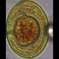
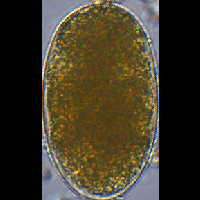
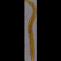
(a) H. Nana	(b) Ancylostomatidae	(c)S. stercoralis
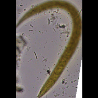
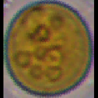
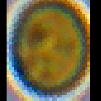
(d) S. stercoralis	(e) E. coli	(f) E. nana
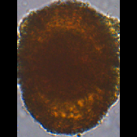
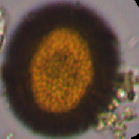
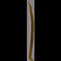
(g) A. lumbricoides	(h) Taenia spp.	(i) S. stercoralis
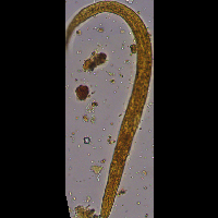
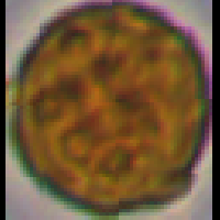
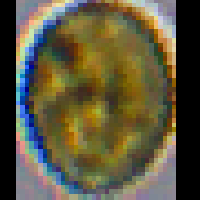
(j) S. stercoralis	(k)E. coli	(l) G. duodenalis

Figure 11: Examples of images (a-f) misclassified by $DS_{1}$, selected, and correctly classified by $DS_{2}$, (g-l) correctly classified by $DS_{1}$, selected, and misclassified by $DS_{2}$.

6 Conclusion

We presented a hybrid approach to combine two decision-making systems with complementary properties — a faster and less accurate decision system $DS_{1}$ with a slower and more accurate decision system $DS_{2}$ — in order to improve overall effectiveness without compromising efficiency and cost in image analysis. We have successfully demonstrated this approach for the diagnosis of the 15 most common species of human intestinal parasites in Brazil. In this application, after exhaustive experiments, the best choices of classifiers for $DS_{1}$ and $DS_{2}$ were $p$-SVM and Vgg-16. The resulting hybrid system also represents a low-cost solution viable for the clinical routine, which makes our contribution relevant for the Public Health system in Brazil.

Our main technical contribution is a method that learns the probability distributions of error per class, given the confidence values of $DS_{1}$ on a validation set during training, to select test samples with higher chances of error for a final characterization and reclassification by $DS_{2}$. We believe this hybrid approach can be useful in several other real applications.

As future work, we intend to investigate methods that can simplify a deep neural network without losing effectiveness, or design a lightweight deep neural network with higher effectiveness. By that, we aim at increasing the number of samples selected for $DS_{2}$, further improving the capability of our hybrid system to process more images per time.

7 Acknowledgments

The authors thank FAPESP (Proc. 2017/12974-0 and 2014/12236-1), Immunocamp Ciência e Tecnologia LTDA, and CNPq (Proc. 303808/2018-7).

References

- [1] WHO Fact Sheets. Soil-transmitted helminth infections. http://www.who.int/news-room/fact-sheets/detail/soil-transmitted-helminth-infections, 2018. [Online; accessed October 24, 2018].
- [2] J. B. de Carvalho, B. M. Dos Santos, J. F. Gomes, C. T. N. Suzuki, S. H. Shimizu, A. X. Falcão, J. C. Pierucci, L. V. S. de Matos, and K. D. S. Bresciani. Tf-test modified: New diagnostic tool for human enteroparasitosis. Journal of clinical laboratory analysis, 30 4:293–300, 2016.
- [3] C. T. N. Suzuki, J. F. Gomes, A. X. Falcão, J. P. Papa, and S. Hoshino-Shimizu. Automatic segmentation and classification of human intestinal parasites from microscopy images. IEEE Transactions on Biomedical Engineering, 60(3):803–812, March 2013.
- [4] C. T. N. Suzuki, J. F. Gomes, A. X. Falcão, S. H. Shimizu, and J. P. Papa. Automated diagnosis of human intestinal parasites using optical microscopy images. In IEEE International Symposium on Biomedical Imaging, pages 460–463, 2013b.
- [5] Ting-Fan Wu, Chih-Jen Lin, and R. C Weng. Probability estimates for multi-class classification by pairwise coupling. Journal of Machine Learning Research, 5(Aug):975–1005, 2004.
- [6] K. Simonyan and A. Zisserman. Very deep convolutional networks for large-scale image recognition. CoRR, abs/1409.1556, 2014.
- [7] Y. Seok Yang, D. K. Park, H. C. Kim, M.-H. Choi, and J.-Y. Chai. Automatic identification of human helminth eggs on microscopic fecal specimens using digital image processing and an artificial neural network. Biomedical Engineering, IEEE Transactions on, 48(6):718–730, 2001.
- [8] Y. P. Ginoris, A. L. Amaral, A. Nicolau, M. A. Z. Coelho, and Ferreira E. C. Development of an image analysis procedure for identifying protozoa and metazoa typical of activated sludge system. Water Research, 41:2581–2589, 2007.
- [9] C. A. B. Castañón, J. S. Fraga, S. Fernandez, A. Gruber, and L. F. Costa. Biological shape characterization for automatic image recognition and diagnosis of protozoan parasites of the genus eimeria. Pattern Recognition, 40:1899–1910, 2007.
- [10] E. Dogantekin, M. Yilmaz, A. Dogantekin, E. Avci, and A. Sengur. A robust technique based on invariant moments - anfis for recognition of human parasite eggs in microscopic images. Expert Systems with Applications, 35(3):728–738, 2008.
- [11] D. Avci and A. Varol. An expert diagnosis system for classification of human parasite eggs based on multi-class svm. Expert Systems with Applications, 36(1):43–48, 2009.
- [12] Gökhan Sengül. Classification of parasite egg cells using gray level cooccurence matrix and knn., 2016.
- [13] Alicia Alva, Carla Cangalaya, Miguel Quiliano, Casey Krebs, Robert H. Gilman, Patricia Sheen, and Mirko Zimic. Mathematical algorithm for the automatic recognition of intestinal parasites. PloS one, 12(4):e0175646, 2017.
- [14] O. T. Nkamgang, D Tchiotsop, H. B. Fotsin, and P. K. Talla. An expert system for assistance in human intestinal parasitosis diagnosis. Biosens Bioelectron Open Acc: BBOA-128., 10:2577–2260, 2018.
- [15] Beaudelaire Saha Tchinda, Michel Noubom, Daniel Tchiotsop, Valerie Louis-Dorr, and Didier Wolf. Towards an automated medical diagnosis system for intestinal parasitosis. Informatics in Medicine Unlocked, 13:101–111, 2018.
- [16] Oscar Takam Nkamgang, Daniel Tchiotsop, Beaudelaire Saha Tchinda, and Hilaire Bertrand Fotsin. A neuro-fuzzy system for automated detection and classification of human intestinal parasites. Informatics in Medicine Unlocked, 13:81 – 91, 2018.
- [17] A. Z. Peixinho, S. B. Martins, J. E. Vargas, A. X. Falcão, J. F. Gomes, and C. T. N. Suzuki. Diagnosis of human intestinal parasites by deep learning. In Computational Vision and Medical Image Processing V: Proceedings of the 5th Eccomas Thematic Conference on Computational Vision and Medical Image Processing (VipIMAGE 2015, Tenerife, Spain, October 19-21, 2015), page 107. CRC Press, 2015.
- [18] J. P. Papa, A. X. Falcão, and C. T. N. Suzuki. Supervised pattern classification based on optimum-path forest. International Journal of Imaging Systems and Technology, 19(2):120–131, 2009.
- [19] A. X. Falcão, J. Stolfi, and R. de Alencar Lotufo. The image foresting transform: theory, algorithms, and applications. IEEE Transactions on Pattern Analysis and Machine Intelligence, 26(1):19–29, Jan 2004.
- [20] R. O. Stehling, M. A. Nascimento, and A. X. Falcão. A compact and efficient image retrieval approach based on border/interior pixel classification. In Proc. of the 11th Intl. Conf. on Information and Knowledge Management (CIKM), pages 102–109, McLean, VA, 2002.
- [21] G. C. S. Ruppert, G. Chiachia, F. P. G. Bergo, F. O. Favretto, C. L. Yasuda, A. Rocha, and A. X. Falc ao. Medical image registration based on watershed transform from greyscale marker and multi-scale parameter search. Computer Methods in Biomechanics and Biomedical Engineering: Imaging & Visualization, 5(2):138–156, 2017.
- [22] Chih wei Hsu, Chih chung Chang, and Chih jen Lin. A practical guide to support vector classification, 2010.