New Approximation Algorithms for Forest Closeness Centrality – for Individual Vertices and Vertex Groups

Abstract

The emergence of massive graph data sets requires fast mining algorithms. Centrality measures to identify important vertices belong to the most popular analysis methods in graph mining. A measure that is gaining attention is forest closeness centrality; it is closely related to electrical measures using current flow but can also handle disconnected graphs. Recently, [Jin et al., ICDM’19] proposed an algorithm to approximate this measure probabilistically. Their algorithm processes small inputs quickly, but does not scale well beyond hundreds of thousands of vertices.

In this paper, we first propose a different approximation algorithm; it is up to two orders of magnitude faster and more accurate in practice. Our method exploits the strong connection between uniform spanning trees and forest distances by adapting and extending recent approximation algorithms for related single-vertex problems. This results in a nearly-linear time algorithm with an absolute probabilistic error guarantee. In addition, we are the first to consider the problem of finding an optimal group of vertices w. r. t. forest closeness. We prove that this latter problem is NP-hard; to approximate it, we adapt a greedy algorithm by [Li et al., WWW’19], which is based on (partial) matrix inversion. Moreover, our experiments show that on disconnected graphs, group forest closeness outperforms existing centrality measures in the context of semi-supervised vertex classification.

Keywords: Forest closeness centrality, group centrality, forest distance, uniform spanning tree, approximation algorithm

1 Introduction

Massive graph data sets with millions of edges (or more) have become abundant. Today, applications come from many different scientific and commercial fields [24, 4]. Network analysis algorithms shall uncover non-trivial relationships between vertices or groups of vertices in these data. One popular concept used in network analysis is centrality. Centrality measures assign to each vertex (or edge) a score based on its structural importance; this allows to rank the vertices and to identify the important ones [7, 33]. Measures that capture not only local graph properties are often more meaningful, yet relatively expensive to compute [32]. Also, different applications may require different centrality measures, none is universal.

Algebraic measures such as random-walk betweenness, electrical closeness (see Refs. in [1, 32]), and forest closeness centrality [18] are gaining increasing attention. Forest closeness is based on forest distance, which was introduced by Chebotarev and Shamis [13] to account not only for shortest paths. Moreover, it applies to disconnected graphs as well. In sociology, forest distances are shown to better capture more than one sensitive relationship index, such as social proximity and group cohesion [12]. Consequently, forest closeness centrality has two main advantages over many other centrality measures [18]: (i) by taking not only shortest paths into account, it has a high discriminative power and (ii) unlike related algebraic measures such as the above, it can handle disconnected graphs out of the box.

Recently, Jin et al. [18] provided an approximation algorithm for forest closeness centrality with nearly-linear time complexity. Their algorithm uses the Johnson-Lindenstrauss transform (JLT) and fast linear solvers; it can handle much larger inputs than what was doable before, but is still time-consuming. For example, graphs with $\approx$1M vertices and $\approx$2-3M edges require more than $2.3$ or $4.7$ hours for a reasonably accurate ranking in their study [18]. Obviously, this hardly scales to massive graphs with $>50$M edges; corresponding applications would benefit significantly from faster approximation methods.

To this end, we devise new approximation algorithms for two problems: first, for the individual forest closeness centrality value of each node – by adapting uniform spanning tree techniques from recent related work on electrical closeness centrality [1, 5]. In a next step, we consider group forest closeness centrality, where one seeks a set of vertices that is central jointly. To the best of our knowledge, we are the first to address the group case for this centrality measure. We prove that group forest closeness is $\mathcal{NP}$-hard and adapt the greedy algorithm by Li et al. [22] to this problem. Our experiments on common benchmark graphs show that our algorithm for ranking individual vertices is always substantially faster than Jin et al.’s [18] – for sufficiently large networks by one (better accuracy) to two (similar accuracy) orders of magnitude in a sequential setting. Our new algorithm can now rank all vertices in networks of up to $334$M edges with reasonable accuracy in less than 20 minutes if executed in an MPI-parallel setting. Also, experiments on semi-supervised vertex classification demonstrate that our new group forest closeness measure improves upon existing measures in the case of disconnected graphs.

2 Definitions and Notation

As input we consider finite and simple undirected graphs $G=(V,E,\mathbf{w})$ with $n$ vertices, $m$ edges, and edge weights $\mathbf{w}\in\mathbb{R}_{\geq 0}^{m}$. By $\mathbf{L}$ we denote the Laplacian matrix of $G$, defined as $\mathbf{L}=\mathbf{diag}(\deg_{G}(1),\ldots,\deg_{G}(n))-\mathbf{A}_{G}$, where $\mathbf{A}_{G}$ denotes the (weighted) adjacency matrix of $G$ and $\deg_{G}(v)$ the (weighted) degree of vertex $v$.

Closeness centrality.

Let $d(u,v)$ denote the graph distance in $G$. The farness of a vertex $u$ is defined as $f^{d}(u):=\sum_{v\neq u}d(u,v)$, i. e., up to a scaling factor of $\frac{1}{n}$, the farness of $u$ quantifies the average distance of $u$ to all other vertices. Given this definition, the closeness centrality of $u$ is defined as $C^{d}(u):=\frac{n}{f^{d}(u)}$. Closeness is a widely used centrality measure; the higher the numerical value of $C^{d}(u)$ is, the more central is $u$ within the graph. It is often criticized for mapping the vertex scores into a rather narrow interval [24].

Forest Distance / Closeness.

Forest distance generalizes the common graph distance and takes not only shortest paths into account [13]. It is expressed in terms of the (parametric) forest matrix of a graph $G$ defined as $\mathbf{\Omega}:=\mathbf{\Omega}_{\alpha}:=(\alpha\mathbf{L}+\mathbf{I})^{-1}$, where $\mathbf{I}$ is the identity matrix and $\alpha>0$ controls the importance of short vs long paths between vertices (some papers prefer the expression $(\mathbf{L}+\alpha\mathbf{I})^{-1}$, which is equivalent to $\mathbf{\Omega}_{\alpha}$ up to scaling; non-parametric variants of forest closeness fix $\alpha$ to $1$ [11]):

Definition 1 (Forest distance [13])

The forest distance $\mathbf{\rho}(u,v)$ for a vertex pair $(u,v)$ is defined as:

(2.1) $$\begin{split}\mathbf{\rho}(u,v)&:=\mathbf{\rho}_{\alpha}(u,v):=(\mathbf{e}_{u}-\mathbf{e}_{v})^{T}\mathbf{\Omega}_{\alpha}(\mathbf{e}_{u}-\mathbf{e}_{v})\\ &=\mathbf{\mathbf{\Omega}_{\alpha}}[u,u]+\mathbf{\mathbf{\Omega}_{\alpha}}[v,v]-2\mathbf{\mathbf{\Omega}_{\alpha}}[u,v].\end{split}$$

Chebotarev and Shamis [13] show that forest distance is a metric and list other desirable properties. The name forest distance stems from the fact that an entry $\mathbf{\mathbf{\Omega}}[u,v]$ equals the fraction of spanning rooted forests in $G$ in which $u$ and $v$ belong to the same tree, see [18]. Forest distance closeness centrality, or forest closeness for short, then uses forest distances instead of the usual graph distance in the sum over all other vertices:

Definition 2 (Forest closeness [13])

The forest farness $\mathbf{\rho}(u)$ of a vertex $u$ is defined as $\mathbf{\rho}(u):=\sum_{v\in V\setminus\{u\}}\mathbf{\rho}(u,v)$. Likewise, the forest distance closeness centrality of $u$ is defined as: $\mathbf{f_{\alpha}}(u):=\frac{n}{\mathbf{\rho}(u)}$.

To simplify notation and when clear from the context, we often omit $\alpha$ in the following.

Effective Resistance and Electrical Closeness.

As already realized by Chebotarev and Shamis [13], there is a close connection between forest distance and effective resistance, a. k. a. resistance distance (more details on this connection in Section 4.1). Effective resistance is a pairwise metric on the vertex set of a graph and also plays a central role in several centrality measures [30, 9]. The notion of effective resistance comes from viewing $G$ as an electrical circuit in which each edge $e$ is a resistor with resistance $1/\mathbf{w}(e)$. Following fundamental electrical laws, the effective resistance $\mathbf{r}(u,v)$ between two vertices $u$ and $v$ (that may or may not share an edge) is the potential difference between $u$ and $v$ when a unit of current is injected into $G$ at $u$ and extracted at $v$. Effective resistance is also proportional to hitting times of random walks [8] and thus has connections to Markov chains. Computing the effective resistance $\mathbf{r}(u,v)$ of a vertex pair $(u,v)\in V\times V$ can be done by means of the Laplacian pseudoinverse $\mathbf{L_{G}}^{\dagger}$ as

(2.2) $$\mathbf{r}(u,v)=\mathbf{\mathbf{L_{G}}^{\dagger}}[u,u]+\mathbf{\mathbf{L_{G}}^{\dagger}}[v,v]-2\mathbf{\mathbf{L_{G}}^{\dagger}}[u,v]$$

(or by solving a Laplacian linear system). Given the definition of $\mathbf{r}(u,v)$, one obtains the well-known definition of electrical closeness by replacing $\mathbf{\rho}(u)$ by $\mathbf{r}(u,v)$ in Definition 2. Electrical closeness (aka current-flow closeness or information centrality) has been widely studied (see e. g., [9, 22, 6, 32]), but only in the context of connected graphs.

3 Related Work

The most relevant algorithmic work regarding forest closeness was proposed by Jin et al. [18], who presented an $\varepsilon$-approximation algorithm for forest distance and forest closeness for all graph nodes. The authors exploit the Johnson-Lindenstrauss lemma [19], thus use random projections and rely on fast Laplacian solvers [14] to avoid matrix inversions. The algorithm has a running time of $\mathcal{O}(m\varepsilon^{-2}\log^{2.5}{n}\log(1/\varepsilon)\operatorname{poly}(\log\log n))$ and provides a $(1\pm\varepsilon)$-approximation guarantee with high probability (assuming an exact Laplacian solver). In practice, as mentioned above, their approach takes $>2$ hours on graphs with $\approx$1M vertices and $\approx$2-3M edges for a reasonably accurate ranking. Our aim is a better algorithmic solution for forest centrality by leveraging our recent results on the approximation of the diagonal entries of $\mathbf{L_{G}}^{\dagger}$ [1]. The latter exploits the connection to effective resistances and electrical closeness and is stated here for completeness:

Proposition 3.1 ([1])

Let $G=(V,E)$ be an undirected and weighted graph with diameter $\operatorname{diam}(G)$ and volume $\operatorname{vol}(G)$. There is an algorithm that computes with probability $1-\delta$ an approximation of $\operatorname{diag}(\mathbf{L_{G}}^{\dagger})$ with absolute error $\pm\varepsilon$ in expected time $\mathcal{O}(\operatorname{vol}(G)\cdot\operatorname{ecc}^{3}(u)\cdot\varepsilon^{-2}\cdot\log(\operatorname{vol}(G)/\delta))$ , where $\operatorname{ecc}(u)$ is the eccentricity of a selected node $u$.

That algorithm exploits three major insights: (i) to compute the electrical closeness of a node $u$, one only needs $\mathbf{\mathbf{L_{G}}^{\dagger}}[u,u]$ and the trace of $\mathbf{L_{G}}^{\dagger}$; (ii) after obtaining the $u$-th column of $\mathbf{L_{G}}^{\dagger}$ (by solving one Laplacian linear system) and all effective resistances $\mathbf{r}(u,v)$ between $u$ and all $v$, the remaining elements of $\operatorname{diag}(\mathbf{L_{G}}^{\dagger})$ can be calculated via Eq. (2.2), (iii) effective resistances can be approximated by sampling uniform spanning trees (USTs), e. g., with Wilson’s algorithm [34], by exploiting Kirchhoff’s theorem. For our purposes, we can state it as the effective resistance of an edge $\{u,v\}\in E$ being the probability that $\{u,v\}$ is in a spanning tree drawn uniformly at random from all spanning trees of $G$ (comp. [8]).

The algorithm proposed in this paper for approximating individual centrality scores is based on the above insights, transfers them to a different graph and provides a new analysis with an improved running time for the case at hand.

Barthelmé et al. [5] proposed an algorithm that uses techniques similar to the ones in Ref. [1] to estimate inverse traces that arise in regularized optimization problems. Their algorithm is based on uniform spanning forests, also sampled with Wilson’s algorithm. Finally, for the group centrality case, the most relevant algorithm is Li et al.’s [22]; it employs JLT and fast Laplacian solvers to approximate group electrical closeness centrality in nearly-linear time.

4 Forest Closeness of Individual Vertices

By definition, forest closeness for a vertex $u$ can be computed from all forest distances $\mathbf{\rho}(u,v)$, $v\in V\setminus\{u\}$, e. g., by matrix inversion. Yet, inversion takes cubic time in practice and is thus impractical for large graphs. Hence, we exploit a relation between forest distance and effective resistance to approximate the forest farness more efficiently than existing approximation algorithms. By adapting our algorithm for electrical closeness [1], we obtain an algorithm with a (probabilistic) additive approximation guarantee of $\pm\varepsilon$; it runs in nearly-linear (in $m$) expected time.

4.1 From Forest Farness to Electrical Farness (And Back Again).

As mentioned, we exploit a result that relates forest distances to effective resistances. This requires the creation of an augmented graph $G_{\star}:=G_{\star,\alpha}:=(V^{\prime},E^{\prime})$ from the original graph $G=(V,E)$. To this end, a new universal vertex $u^{\star}$ is added to $G$, such that $V^{\prime}=V\cup\{u^{\star}\}$ and $E^{\prime}=E\cup\{u^{\star},v\},~{}\forall v\in V$. In particular, $u^{\star}$ is connected to all other vertices of $G_{\star}$ with edges of weight one. Furthermore, the weights of all edges in $E^{\prime}$ that belong to $E$ are multiplied by $\alpha$.

Proposition 4.1 (comp. Ref. [13])

For a weighted graph $G=(V,E)$ and any vertex pair $(v_{1},v_{2})\in V\times V$, the forest distance $\mathbf{\rho}(v_{1},v_{2})$ in $G$ equals the effective resistance $\mathbf{r}(v_{1},v_{2})$ in the augmented graph $G_{\star}$.

The full proof of Proposition 4.1 can be found in Ref. [13]. Nevertheless, we provide here an explanation of why the above proposition holds. Recall that the effective resistance between any two vertices of $G$ is computed by means of $\mathbf{L_{G}}^{\dagger}$, while the forest distances of the same pair are computed by means of the forest matrix of $G$, $\mathbf{\mathbf{\Omega}}=(\alpha\mathbf{L}+\mathbf{I})^{-1}$. When calculating the effective resistance in $G_{\star}$, we use its Laplacian matrix $\mathbf{L}_{\star}$, which consists of a block matrix corresponding to $(\alpha\mathbf{L}+\mathbf{I})$ and an additional row and column that corresponds to the universal vertex $u^{\star}$. It turns out that the Moore-Penrose pseudoinverse of $\mathbf{L}_{\star}$ is the block matrix that consists of $\mathbf{\Omega}$ with an additional row and column corresponding to $u^{\star}$ [13]. Thus, $\mathbf{\mathbf{\Omega}}[u^{\star},u^{\star}]+\mathbf{\mathbf{\Omega}}[v,v]-2\mathbf{\mathbf{\Omega}}[u^{\star},v]$ equals $\mathbf{\mathbf{L}_{\star}^{\dagger}}[u^{\star},u^{\star}]+\mathbf{\mathbf{L}_{\star}^{\dagger}}[v,v]-2\mathbf{\mathbf{L}_{\star}^{\dagger}}[u^{\star},v]$, which corresponds to the pairwise effective resistance $\mathbf{r}(u^{\star},v)$ in $G_{\star}$.

Corollary 4.1

Forest closeness in graph $G$ equals electrical closeness in the augmented graph $G_{\star}$.

4.2 Forest Farness Approximation Algorithm.

As mentioned, our new algorithm for forest closeness exploits previous algorithmic results for approximating $\operatorname{diag}(\mathbf{L_{G}}^{\dagger})$ and electrical closeness. To do so, we rewrite forest farness $\mathbf{\rho}(v)$ following Ref. [23]:

(4.3) $$\begin{split}\mathbf{\rho}(v)&=n\cdot\mathbf{\mathbf{\Omega}}[v,v]+\operatorname{tr}(\mathbf{\Omega})-2\sum_{w\in V}\mathbf{\mathbf{\Omega}}[v,w]\\ &=n\cdot\mathbf{\mathbf{\Omega}}[v,v]+\operatorname{tr}(\mathbf{\Omega})-2,\end{split}$$

where the last equation holds since $\mathbf{\Omega}$ is doubly stochastic ($\mathbf{\mathbf{\Omega}}[v,v]=1-\sum_{w\neq v}\mathbf{\mathbf{\Omega}}[v,w]$) [23]. From Eq. (4.3) it is clear that we only require the diagonal elements of $\mathbf{\Omega}$ to compute $\mathbf{\rho}(v)$ for any $v\in V$. We approximate the diagonal elements of $\mathbf{\Omega}$ with Algorithm 1, whose main idea is to sample uniform spanning trees (USTs) to approximate $\operatorname{diag}(\mathbf{L}_{\star}^{\dagger})$:

1. We build the augmented graph $G_{\star}$ (Line 4) and let the universal vertex $u^{\star}$ of $G_{\star}=(V^{\prime},E^{\prime})$ be the so-called pivot vertex (Line 5) – due to its optimal eccentricity of $1$. Later, we compute the column of $\mathbf{\Omega}$ that corresponds to $u^{\star}$, $\mathbf{\mathbf{\Omega}}[:,u^{\star}]$, by solving the Laplacian linear system $\mathbf{L}_{\star}\mathbf{x}=\mathbf{e}_{u^{\star}}-\frac{1}{n+1}\cdot\mathbf{1}$ (Line 11). The solver’s accuracy is controlled by $\eta$, which is set in Line 7 ($\kappa$ is used to trade the accuracy of the solver with the accuracy of the following sampling step).

2. We sample $\tau$ USTs in $G_{\star}$ with Wilson’s algorithm [34] (also see Algorithm 3 in Section B), where the sample size $\tau$ is yet to be determined. With this sample we approximate the effective resistance $\mathbf{r}_{G_{\star}}(u^{\star},v)$ for all $v\in V$ (Lines 9-10). More precisely, if an edge $\{u^{\star},v\}$ appears in the sampled tree, we increase $R[v]$ by $1$ (unweighted case) or by the weight of the current tree (weighted case) – and later “return” $R[v]/\tau$ (unweighted case) or the relative total weight of all sampled trees (weighted case) that contain edge $\{u^{\star},v\}$ in Line 13.

3. We compute the remaining $\mathbf{\mathbf{\Omega}}[v,v]$ for $v\in V$ in Lines 12 and 13 following Eqs. (2.1) and (2.2):

   $$\mathbf{\mathbf{\Omega}}[v,v] =\mathbf{\rho}(u^{\star},v)-\mathbf{\mathbf{\Omega}}[u^{\star},u^{\star}]+2\mathbf{\mathbf{\Omega}}[v,u^{\star}]$$

   $$=\mathbf{r}_{G_{\star}}(u^{\star},v)-\mathbf{\mathbf{\Omega}}[u^{\star},u^{\star}]+2\mathbf{\mathbf{\Omega}}[v,u^{\star}],$$

   where $\mathbf{r}_{G_{\star}}(u^{\star},v)$ is then approximated by $R[v]/\tau$ (the weighted case is handled as described above).

1:function ApproxDiagForestMatrix($G$, $\alpha$, $\varepsilon$, $\delta$)

2:    Input: Undir. graph $G=(V,E)$, control parameter $\alpha$, error bound $0<\varepsilon<1$, probability $0<\delta<1$

3:    Output: $\operatorname{diag}(\widetilde{\mathbf{\Omega}})$, i. e., an $(\varepsilon,\delta)$-approximation of $\operatorname{diag}(\mathbf{\Omega})$

4:    Create augmented graph $G_{\star}=(V^{\prime},E^{\prime})$ as described in Proposition 4.1; compute $\operatorname{vol(G)}$ and $c$ $\triangleright$ $\mathcal{O}(m+n)$

5:    $u^{\star}\leftarrow$ universal vertex of $G_{\star}$

6:    Pick constant $\kappa\in(0,1)$ arbitrarily

7:    $\eta\leftarrow\frac{\kappa\varepsilon}{6\sqrt{\alpha(c+2)\operatorname{vol}(G)}}$

8:    $\tau\leftarrow\lceil\log(2m/\delta)/2(1-\kappa)^{2}\varepsilon^{2}\rceil$

9:    for $i\leftarrow 1$ to $\tau$ do $\triangleright$ $\tau$ times

10:         $R\leftarrow$ SamplingUST($G_{\star}$, $u$) $\triangleright$ $\mathcal{O}(\alpha\operatorname{vol}(G)+n)$     

11:    Solve $\mathbf{L}_{\star}\mathbf{x}=\mathbf{e}_{u^{\star}}-\frac{1}{n+1}\cdot\mathbf{1}$ for $\mathbf{x}$ $\triangleright$ accuracy: $\eta$, $\tilde{\mathcal{O}}(m\log^{1/2}n\log(1/\eta))$

12:    for $v\in V$ do $\triangleright$ All iterations: $\mathcal{O}(n)$

13:          $\mathbf{\widetilde{\mathbf{\Omega}}}[v,v]\leftarrow R[v]/\tau-\mathbf{x}(u^{\star})+2\mathbf{x}(v)$ $\triangleright$ unweighted case, for weighted see text     

14:    return $\operatorname{diag}(\widetilde{\mathbf{\Omega}})$

Algorithm 1 Approximation algorithm for $\operatorname{diag}(\mathbf{\Omega})$

By using $G_{\star}$ and thus a universal vertex $u^{\star}$ as pivot, there are several noteworthy changes compared to the algorithm in Ref. [1]. First, the graph $G_{\star}$ has constant diameter and the vertex $u^{\star}$ constant eccentricity $1$. This will be important for our refined running time analysis. Second, the approximation of the effective resistances can be simplified: while Ref. [1] requires an aggregation along shortest paths, we notice that here $u^{\star}$ and all other vertices are connected by paths of one edge only; thus, the relative frequency of an edge $\{u^{\star},v\}$ in the UST sample for $G_{\star}$ is sufficient here for our approximation:

Proposition 4.2

Let $u^{\star}$ be the universal vertex in $G_{\star}$. Then, for any edge $\{u^{\star},v\}\in E^{\prime}$ holds: its relative frequency (or weight) in the UST sample is an unbiased estimator for $\mathbf{r}_{G_{\star}}(u^{\star},v)$.

The proof of Proposition 4.2 relies on Kirchhoff’s theorem (see [8, Ch. II]) and can be found in Section A.

As we will see in our main algorithmic result (Theorem 4.1), Algorithm 1 is not only an unbiased estimator, but even provides a probabilistic approximation guarantee. To bound its running time, we analyze Wilson’s algorithm for generating a UST first.

Proposition 4.3

For an undirected graph $G$ with constant diameter, each call to Wilson’s algorithm on $G_{\star}$ (in Line 10) takes $\mathcal{O}(\alpha\operatorname{vol}(G)+n)$ expected time, where $\operatorname{vol}(G)=\sum_{v\in V}\deg(v)$ is the (possibly weighted) volume of $G$.

The proof of Proposition 4.3 can be found in Section A. Note that in the case of unweighted graphs with $\alpha=1$ and $m=\Omega(n)$ (which is not uncommon in our context, see for example Ref. [18]), we obtain a time complexity of $\mathcal{O}(m)$ (the volume is $2m$ by the handshake lemma). Taking all the above into account, we arrive at our main algorithmic result on running time and approximation bounds of Algorithm 1. The result and its proof are adaptations of Theorem 3 in Ref. [1]. When considering forest (as opposed to electrical) closeness centrality, we exploit the constant diameter of $G_{\star}$ and improve the time by a factor of $(\operatorname{ecc}(u))^{3}$, where $u$ is a selected pivot node. This expression is $\mathcal{O}(\log^{3}n)$ for the small-world graphs in the focus of Ref. [1] (but can be larger for general graphs). In the following, $\tilde{\mathcal{O}}(\cdot)$ hides polyloglog factors from the linear solver [14].

Theorem 4.1

Let $\frac{n}{\alpha\cdot\operatorname{vol}(G)}$ be bounded from above by a constant and let $0<\varepsilon,\delta<1$. Then, with probability $1-\delta$, Algorithm 1 computes an approximation of $\operatorname{diag}(\mathbf{\Omega})$ with absolute error $\pm\varepsilon$ in (expected) time $\tilde{\mathcal{O}}((m\log^{1/2}n\log(\sqrt{\alpha\operatorname{vol}(G)}/\varepsilon)))+\mathcal{O}(\log(n/\delta)/\varepsilon^{2}\cdot\alpha\operatorname{vol}(G))$.

Theorem 4.1 is proved in Section A. Let us simplify the result for a common case:

Corollary 4.2

If $G$ is unweighted, $\alpha$ a constant and $\delta:=1/n$ to get high probability, the (expected) running time of Algorithm 1 becomes $\tilde{\mathcal{O}}(m(\log^{1/2}n\log(n/\varepsilon)+\varepsilon^{-2}\log n))$. Assuming $\varepsilon$ is small enough so that $\log n\leq 1/\varepsilon$, we can further simplify this to $\tilde{\mathcal{O}}(m\varepsilon^{-2}\log^{3/2}n)$.

This is nearly-linear in $m$, which is also true for the JLT-based approximation (with high probability) of Jin et al. [18]. They state a running time of $\tilde{\mathcal{O}}(m\varepsilon^{-2}\log^{5/2}n\log(1/\varepsilon))$ for unweighted $G$ and fixed $\alpha=1$. While we save at least a factor of $\log n$, they achieve a relative approximation guarantee, which is difficult to compare to ours.

5 Group Forest Closeness Centrality

Since their introduction by Everett and Borgatti [15], group centrality measures have been used in various applications (see [32]). These measures indicate the importance of whole vertex sets – together as a group. They usually favor sets that “cover” the graph well. Intuitively, a group variant of forest closeness should reward vertex sets that are “forest-close” to the remainder of the graph. More formally, to extend the concept of forest closeness to groups of vertices, it is enough to define the forest farness $\mathbf{\rho}(S)$ of a set $S$ of vertices; the forest closeness of $S$ is then given by $\mathbf{f_{\alpha}}(S):=\frac{1}{\mathbf{\rho}(S)}$. Recall (from Proposition 4.1) that the forest farness of a single vertex $v$ of $G$ is identical to the electrical farness of $v$ in the augmented graph $G_{\star}$. We use this fact to generalize the forest farness of a set $S$ of vertices of $G$. In particular, we define $\mathbf{\rho}(S):=\operatorname{tr}((\left(\mathbf{L}_{\star}\right)_{-S})^{-1})$, where $\mathbf{L}_{\star}$ is the Laplacian matrix of the augmented graph $G_{\star}$ and by $\left(\mathbf{L}_{\star}\right)_{-S}$ we denote the matrix that is obtained from $\mathbf{L}_{\star}$ by removing all rows and columns with indices in $S$. This definition is based on a corresponding definition of electrical farness by Li et al. [22]. For $|S|=1$, it coincides with the definition of electrical closeness from Section 2  [17]; thus, our definition of group forest closeness is compatible with the definition of the forest closeness of individual vertices (i. e., Definition 2).

Given our definition, it is natural to ask for a set $S$ of $k$ vertices that maximizes $\mathbf{f_{\alpha}}(S)$ over all possible size-$k$ sets $S$; indeed, this optimization problem has also been considered for many other group centrality measures [32]. The following theorem settles the complexity of the problem:

Theorem 5.1

Maximizing GroupForestCloseness subject to a cardinality constraint is $NP$-hard.

As Li et al.’s [22] hardness proof for group electrical closeness, our reduction is from the vertex cover problem on 3-regular graphs. Let $G=(V,E)$ be a 3-regular graph with $n$ vertices. Our proof shows that there is a vertex cover of size $k$ in $G$ if and only if the maximum group forest closeness over all sets of size $k$ in $G$ exceeds a certain threshold. We make use of the following property that is adapted from a similar result by Li et al.:

Lemma 5.1

Let $G$ be a connected and unweighted 3-regular graph and let $S\subset V$, $|S|=k\geq 1$. Then $\operatorname{tr}((\left(\mathbf{L}\right)_{-S}+\mathbf{I})^{-1})\geq(n-k)/4$ and equality holds if and only if $S$ is a vertex cover of $G$.

Our proof of Theorem 5.1 exploits the fact that we can decompose $\left(\mathbf{L}_{\star}\right)_{-S}$ into a block that corresponds to the universal vertex of $G_{\star}$ and into a block that equals $\left(\mathbf{L}\right)_{-S}+\mathbf{I}$. This allows us to apply the block-wise inversion and the Sherman-Morrison formula to partially invert $\left(\mathbf{L}_{\star}\right)_{-S}$. In turn, we can apply Lemma 5.1 to bound $\operatorname{tr}((\left(\mathbf{L}_{\star}\right)_{-S})^{-1})$. The proof of Lemma 5.1 and the full proof of Theorem 5.1 can be found in Section A.

Since an efficient algorithm for maximizing group forest closeness is unlikely to exist (due to Theorem 5.1), it is desirable to construct an inexact algorithm for this problem. The next two results enable the construction of such an algorithm; they follow immediately from respective results on group electrical closeness on $G_{\star}$ (see Ref. [22, Theorem 5.4 and Theorem 6.1]).

Lemma 5.2

$\mathbf{\rho}(.)$ is a non-increasing and supermodular set function.

For the following corollary, we consider a greedy algorithm that constructs a set $S$ of size $k$. This set is initially empty; while $|S|$ is smaller than $k$, the algorithm adds the vertex $v$ to $S$ that maximizes the marginal gain: $v=\operatorname{argmax}_{x\in V\setminus S}\mathbf{\rho}(S)-\mathbf{\rho}(S\cup\{v\})$.

Corollary 5.1

The greedy algorithm computes a set $S$ such that:

$$\mathbf{\rho}(\{v_{0}\})-\mathbf{\rho}(S)\geq\left(1-\frac{k}{e(k-1)}\right)\left(\mathbf{\rho}(v_{0})-\mathbf{\rho}(\widetilde{S})\right),$$

where $v_{0}$ is the vertex with highest (individual) forest closeness and $\widetilde{S}$ is the set of size $k$ that maximizes group forest closeness.

1:Input: Undir. graph $G=(V,E)$, group size $k$

2:Output: Group $S\subseteq V$ of $k$ vertices

3:$\mathbf{P}\leftarrow\textsc{pseudoInverse}(\mathbf{L}_{\star})$

4:$v\leftarrow\operatorname{argmin}_{v\in V}n(\mathbf{L}_{\star}^{\dagger}[v,v])+\operatorname{tr}(\mathbf{P})$

5:$\mathbf{M}\leftarrow\textsc{inverse}(\left(\mathbf{L}_{\star}\right)_{-\{v\}})$ $\triangleright$ Invariant: $\mathbf{M}\leftarrow\left(\mathbf{L}_{\star}\right)_{-S}^{-1}$ throughout the algorithm

6:$S\leftarrow\{v\}$

7:while $|S|\leq k$ do

8:     $v\leftarrow\operatorname{argmax}_{v\in V\setminus S}\frac{(\mathbf{M}e_{v})^{T}(\mathbf{M}e_{v})}{e_{v}^{T}\mathbf{M}e_{v}}$

9:     $\mathbf{M}\leftarrow\left(\mathbf{M}-\frac{\mathbf{M}e_{v}e_{v}^{T}\mathbf{M}}{e_{v}^{T}\mathbf{M}e_{v}}\right)_{-\{v\}}$

10:     $S\leftarrow S\cup\{v\}$

Algorithm 2 Greedy algorithm for group forest closeness maximization adapted from Li et al.

Note that a naïve implementation of the greedy algorithm would invert $\left(\mathbf{L}_{\star}\right)_{-(S\cup\{v\})}$ for each $v$, i. e., it would require $k\cdot n$ matrix inversions in total. By using the ideas of Li et al. for group electrical closeness [22] (depicted in Algorithm 2 for the case of group forest closeness), these inversions can be avoided, such that only a single matrix inversion is required in total. This makes use of the fact that whenever a vertex $u$ is added to the set $S$, we can decompose $\left(\mathbf{L}_{\star}\right)_{-S}$ into a block that consists of $\left(\mathbf{L}_{\star}\right)_{-(S\cup\{u\})}$ and a single row/column that corresponds to $u$. It is now possible to apply block-wise matrix inversion to this decomposition to avoid the need to recompute $(\left(\mathbf{L}_{\star}\right)_{-(S\cup\{u\})})^{-1}$ from scratch (in line 9 of the pseudocode). We remark that the greedy algorithm can be further accelerated by utilizing the Johnson-Lindenstrauss lemma [22]; however, since this necessarily results in lower accuracy, we do not consider this extension in our experiments.

Furthermore, we note that by applying a standard reduction by Gremban [16], it would also be possible to apply our UST-based algorithm (i. e., Algorithm 1) to the case of group forest closeness. However, if the aforementioned block-wise matrix inversion is not applied, this would require us to sample USTs for each of the $k\cdot n$ vertex evaluations. On the other hand, in order to apply block-wise inversion, the entire inverse of $\left(\mathbf{L}_{\star}\right)_{-S}$ must be available (and not only the diagonal). Computing this inverse via UST sampling is prohibitively expensive so far. Hence, in our experiments, we prefer the algorithmic approach by Li et al. (adapted for group forest closeness).

6 Experiments

We study the empirical performance of our algorithms on real-world graphs and their impact on graph mining tasks.

Settings.

Unless stated otherwise, all algorithms are implemented in C++, using the NetworKit [29] graph APIs. All experiments are conducted on Intel Xeon Gold 6126 machines with $2\times 12$ cores and 192 GiB of RAM each. Unless stated otherwise, all experiments run on a single core. To ensure reproducibility, all experiments are managed by the SimExPal [2] software. For the evaluation, we use a large collection of undirected graphs of different sizes, coming from a diverse set of domains. All graphs have been downloaded from the public repositories KONECT [20], OpenStreetMap and NetworkRepository [26]. We denote our proposed algorithm for forest closeness by UST and set $\alpha=1$ (as done in Ref. [18]) in all experiments.

Competitors.

For the forest closeness of individual vertices, the main competitor is the JLT-based algorithm by Jin et al. [18], which uses the Laplacian solver from Ref. [21]. We compare against two implementations of this algorithm; one provided by the authors written in Julia v1.0.2 and our own implementation based on Eigen’s CG algorithm. We denote them by JLT-Julia and JLT-CPP, respectively. Like in Ref. [18], we compute the number of linear sytems for JLT-Julia and JLT-CPP as $\left\lceil\frac{\log n}{\varepsilon^{2}}\right\rceil$ (which gives an $\varepsilon\cdot c$ approximation for a fixed constant $c>1$).

6.1 Performance of UST.

We measure now the performance of UST compared to the state-of-the art competitors. Each method is executed with multiple settings of its respective quality parameter.

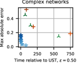
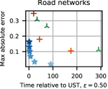
Figure 1: $\max_{u}|\mathbf{\Omega}[v,v]-\widetilde{\mathbf{\Omega}}[v,v]|$ over the instances in Table 1.

Accuracy and Running Time.

We report the maximum absolute error of the estimated diagonal values (i. e., $\max_{v}|\mathbf{\Omega}[v,v]-\widetilde{\mathbf{\Omega}}[v,v]|$) over all vertices and instances from Table 1. As ground truth, we take $\mathbf{\Omega}[v,v]$ values that are computed using Eigen’s CG solver with a tolerance of $10^{-9}$; exact inversion of $(\mathbf{L}+\mathbf{I})$ would be infeasible for many of the input graphs. A preliminary comparison against the values of $\mathbf{\Omega}[v,v]$ computed with the NumPy pinv function demonstrated that CG provides a sufficiently accurate ground truth.

Figure 1 shows that UST achieves the best results in terms of quality and running time for both complex and road networks. More precisely, for complex networks and $\varepsilon=0.4$, UST yields a maximum absolute error of $\numprint{0.14}$, which is less than the most accurate result of both competitors ($\numprint{0.15}$ achieved by JLT-Julia with $\varepsilon=0.1$), while being $\numprint{397.5}\times$ faster. Also, the running time of UST does not increase substantially for lower values of $\varepsilon$, and its quality does not deteriorate quickly for higher values of $\varepsilon$. A similar pattern is observed for road networks as well.

Complex networks

Graph	$|V|$	$|E|$	Time (s)		KT
			UST	JLT	UST	JLT
loc-brightkite_edges	58K	214K	46.4	186.4	0.98	0.95
douban	154K	327K	80.8	370.9	0.71	0.61
soc-Epinions1	75K	405K	55.5	339.6	0.95	0.90
slashdot-zoo	79K	467K	59.9	412.3	0.95	0.92
petster-cat-household	105K	494K	61.8	372.1	0.98	0.92
wikipedia_link_fy	65K	921K	58.2	602.9	0.98	0.96
loc-gowalla_edges	196K	950K	230.9	1,215.5	0.99	0.97
wikipedia_link_an	56K	1.1M	50.7	562.6	0.96	0.93
wikipedia_link_ga	55K	1.2M	44.8	578.6	0.98	0.97
petster-dog-household	260K	2.1M	359.6	2,472.1	0.98	0.96
livemocha	104K	2.2M	107.4	1,429.3	0.98	0.97

Road networks

Graph	$|V|$	$|E|$	Time (s)		KT
			UST	JLT	UST	JLT
mauritania	102K	150K	98.1	217.6	0.88	0.77
turkmenistan	125K	165K	118.5	273.6	0.92	0.85
cyprus	151K	189K	149.4	315.8	0.89	0.80
canary-islands	169K	208K	185.5	382.0	0.92	0.84
albania	196K	223K	192.6	430.2	0.90	0.82
benin	177K	234K	188.1	406.8	0.92	0.83
georgia	262K	319K	322.1	605.3	0.91	0.83
latvia	275K	323K	355.2	665.4	0.91	0.83
somalia	291K	409K	420.1	747.5	0.92	0.84
ethiopia	443K	607K	825.9	1,209.7	0.91	0.83
tunisia	568K	766K	1,200.1	1,629.0	0.89	0.79

Table 1: Running time and KT ranking scores of UST and JLT-based algorithms. In the JLT column we report, for each instance, the competitor with highest KT score. For equal KT scores (up to the second decimal place) we choose the fastest competitor.

Vertex Ranking.

Moreover, we measure the accuracy in terms of vertex rankings, which is often more relevant than individual scores [24, 25]. In Table 1 we report the Kendall’s rank correlation coefficient (KT) of the vertex ranking w. r. t.  the ground truth along with running times for complex and road networks. For each instance, we pick the best run, i. e., the UST and JLT columns display the run with highest respective KT value. If the values are the same up to the second decimal place, we pick the fastest one. UST has consistently the best vertex ranking scores; at the same time, it is faster than the competitors. In particular, UST is on average $\numprint{7.6}\times$ faster than the JLT-based approaches on complex networks and $\numprint{1.9}\times$ faster on road networks.

Parallel Scalability.

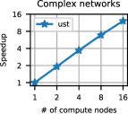
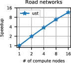
Figure 3: Geometric mean of the speedup of UST with $\varepsilon=\numprint{0.1}$ on multiple compute nodes over a single compute node ($1\times 24$ cores). Data points are aggregated over the instances in Table 2.

UST is well-suited for parallel implementations since each UST can be sampled independently in parallel. Hence, we provide parallel implementations of UST based on OpenMP (for multi-core parallelism) and MPI (to scale to multiple compute nodes). The OpenMP implementation on 24 cores exhibits a speedup of $\numprint{8.7}\times$ on complex networks and $\numprint{9.2}\times$ on road networks – more detailed results can be found in Figure 5, Section C. The results for MPI are depicted in Figure 3, Section C. In this setting, UST obtains a speedup of $\numprint{12.2}\times$ on complex and $\numprint{11.5}\times$ on road networks on up to 16 compute nodes – for this experiment we set $\varepsilon=0.1$ and we use the instances in Table 2, Section C. More sophisticated load balancing techniques are likely to increase the speedups in the MPI setting; they are left for future work. Still, the MPI-based algorithm can rank complex networks with up to $334$M edges in less than $20$ minutes. Road networks with $31$M edges take less than $25$ minutes.

6.2 Semi-Supervised Vertex Classification.

To demonstrate the relevance of group forest closeness in graph mining applications, we apply them to semi-supervised vertex classification [31]. Given a graph $G$ with labelled vertices, the goal is to predict the labels of all vertices of $G$ by training a classifier using a small set of labelled vertices as training set. The choice of the vertices for the training set can influence the accuracy of the classifier, especially when the number of labelled vertices is small compared to $|V|$ [28, 3].

A key aspect in semi-supervised learning problems is the so-called cluster assumption i. e., vertices that are close or that belong to the same cluster typically have the same label [35, 10]. Several models label vertices by propagating information through the graph via diffusion [31]. We expect group forest closeness to cover the graph more thoroughly than individual forest closeness. Hence, we conjecture that choosing vertices with high group centrality improves diffusion and thus the accuracy of propagation-based models. We test this hypothesis by comparing the classification accuracy of the label propagation model [31, 35] where the training set is chosen using different strategies. The main idea of label propagation is to start from a small number of labelled vertices and each vertex iteratively propagates its label to its neighbors until convergence.

In our experiments, we use the Normalized Laplacian variant of label propagation [35]. We set the return probability hyper-parameter to $0.85$, and we evaluate its accuracy on two well-known disconnected graph datasets: Cora ($|V|=\numprint{2708},|E|=\numprint{5278}$) and Citeseer($|V|=\numprint{3264},|E|=\numprint{4536}$) [27]. Since this variant of label propagation cannot handle graphs with isolated vertices (i. e., zero-degree vertices), we remove all isolated vertices from these datasets. For a fixed size $k$ of the training set, we select its vertices as the group of vertices computed by our greedy algorithm for group forest maximization and as the top-$k$ vertices with highest estimated forest closeness. We include several well-known (individual) vertex selection strategies for comparison: average over 10 random trials, the top-$k$ vertices with highest degree, the top-$k$ vertices with highest betweenness centrality and the top-$k$ vertices with highest Personalized PageRank.

Figure 2 shows that on graphs with disconnected components and for a moderate number of labelled vertices, selecting the training set by group forest closeness maximization yields consistently superior accuracy than strategies based on existing centrality measures (including top-$k$ forest closeness). As expected, the accuracy of existing measures improves if one considers connected graphs (Figure 6, Section C); yet, group forest closeness is nearly as accurate as the best competitors on these graphs.

The running time of our greedy algorithm for group forest maximization is reported in Table 3, Section C.

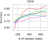
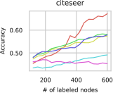
Figure 2: Accuracy in semi-supervised vertex classification when using different strategies to create the training set.

7 Conclusions

In this paper, we proposed a new algorithm to approximate forest closeness faster and more accurately than previously possible. We also generalized the definition of forest closeness to group forest closeness and demonstrated that for semi-supervised vertex classification in disconnected graphs, group forest closeness outperforms existing approaches. In future work, we want to consider extensions of our approaches to directed graphs. Another challenging extension would involve generalizing an approach based on USTs to group forest closeness to improve upon the performance of our greedy algorithm.

A Technical Proofs

• (Proposition 4.2) Since $\{u^{\star},v\}\in E^{\prime}$, we have in the unweighted case that $\mathbf{r}_{G_{\star}}(u^{\star},v)$ is the number of spanning trees of $G_{\star}$ that contain $\{u^{\star},v\}$ divided by the number of all spanning trees of $G_{\star}$ (follows from Kirchhoff’s theorem, see [8, Ch. II]). In the weighted case, replace “number” by “total weight”, respectively (where the weight of a UST is the product of all edge weights). We focus on the unweighted case in the following for ease of exposition; the proof for the weighted case works in the same way.

  Clearly, $R[v]/\tau$, as used by Algorithm 1, is an estimator for $\mathbf{r}_{G_{\star}}(u^{\star},v)$. It remains to show that it is unbiased, i. e., ${\mathbb{E}}[R[v]/\tau]=\mathbf{r}_{G_{\star}}(u^{\star},v)$. To this end, let $T_{i}$ be the UST sampled in iteration $i$ and $X_{i,v}$ the random indicator variable with $X_{i,v}=1$ if $\{u^{\star},v\}\in T_{i}$ and $0$ otherwise. Then:

  $${\mathbb{E}}[R[v]/\tau] =\frac{1}{\tau}{\mathbb{E}}[R[v]]=\frac{1}{\tau}\sum_{i=1}^{\tau}\mathbb{P}[\{u^{\star},v\}\in T_{i}]\cdot X_{i,v}$$

  $$=\frac{1}{\tau}\sum_{i=1}^{\tau}\mathbf{r}_{G_{\star}}(u^{\star},v)\cdot 1=\mathbf{r}_{G_{\star}}(u^{\star},v),$$

  which follows from the definition of expectation and the above correspondence between (the relative frequency of an edge in) USTs and effective resistances.         

• (Proposition 4.3) By plugging the augmented graph $G_{\star}$ (with constant diameter) into the proof of Lemma 10 of Ref. [1], we obtain for the running time $W(n)$ on a graph with $n$ vertices: $W(n)=\mathcal{O}(\operatorname{vol}(G_{\star}))=\mathcal{O}(\alpha\operatorname{vol}(G)+n)$ expected time per call in Line 10.         

• (Theorem 4.1) For the linear system in Line 11, we employ the SDD solver by Cohen et al. [14]; it takes $\tilde{\mathcal{O}}(m\log^{1/2}n\log(1/\eta))$ time to achieve a relative error bound of $\|\mathbf{\tilde{x}}-\mathbf{x}\|_{\mathbf{L^{\prime}}}$, where $\mathbf{L^{\prime}}:=\alpha\mathbf{L}+\mathbf{I}$. We can express the equivalence of this matrix-based norm with the maximum norm by adapting Lemma 12 of Ref. [1] with the norm for $\mathbf{L^{\prime}}$ (instead of $\mathbf{L}$): $\sqrt{\mu_{1}}\cdot\|\mathbf{x}\|_{\infty}\leq\|\mathbf{x}\|_{\mathbf{L^{\prime}}}\leq\sqrt{\alpha(c+2)\operatorname{vol}(G)}\|\mathbf{x}\|_{\infty}$, where $\mu_{1}$ is the smallest eigenvalue of $\mathbf{L^{\prime}}$. In fact, $\mu_{1}=\alpha\lambda_{1}+1=1$, where $\lambda_{1}=0$ is the smallest eigenvalue of $\mathbf{L}$, so that we can simplify:

  (A.1) $$\|\mathbf{x}\|_{\infty}\leq\|\mathbf{x}\|_{\mathbf{L^{\prime}}}\leq\sqrt{\alpha(c+2)\operatorname{vol}(G)}\|\mathbf{x}\|_{\infty}.$$

  Let us set $c:=\frac{n}{\alpha\cdot\operatorname{vol}(G)}$; by our assumption in the theorem, $c$ is a constant. Hence, if we set $\eta:=\kappa\varepsilon/6\sqrt{\alpha(c+2)\operatorname{vol}(G)}$, the SDD solver’s accuracy can be bounded by:

  $$\|\mathbf{\tilde{x}}-\mathbf{x}\|_{\infty} \leq\|\mathbf{\tilde{x}}-\mathbf{x}\|_{\mathbf{L^{\prime}}}\leq\eta\cdot\|\mathbf{x}\|_{\mathbf{L^{\prime}}}$$

  $$\leq\eta\sqrt{\alpha(c+2)\operatorname{vol}(G)}\|\mathbf{x}\|_{\infty}$$

  $$=\frac{\kappa\varepsilon}{6}\|\mathbf{x}\|_{\infty}\leq\frac{\kappa\varepsilon}{3}.$$

  The last inequality follows from the fact that the values in $\mathbf{x}$ are bounded by the effective resistance, which in turn is bounded by the graph distance and thus $2$ (via the edges to/from $u$). If each entry has accuracy of $\kappa\varepsilon/3$ (or better), then Eq. (2.1) is solved with accuracy $\kappa\varepsilon$ (or better). The resulting running time for the SDD solver is thus $\tilde{\mathcal{O}}(m\log^{1/2}n\log(1/\eta))=\tilde{\mathcal{O}}(m\log^{1/2}n\log(\sqrt{\alpha\operatorname{vol}(G)}/\varepsilon))$.

  According to Proposition 4.3 and with $n\leq c\cdot\alpha\cdot\operatorname{vol}(G)$, sampling one UST takes $\mathcal{O}(\alpha\operatorname{vol}(G))$ expected time. It remains to identify a suitable sample size $\tau$ for the approximation to hold. To this end, let $\varepsilon^{\prime}:=(1-\kappa)\varepsilon$ denote the tolerable absolute error for the UST-based approximation part. Plugging $\tau:=\lceil\log(2m/\delta)/2(\varepsilon^{\prime})^{2}\rceil$ into the proof of Theorem 3 of Ref. [1] (and thus essentially Hoeffding’s bound) with the fact that the eccentricity of $u$ is $1$, we obtain the desired result.         

• (Lemma 5.1) The proof in Li et al. [22, Lemma 4.1] exploits (among others) that the diagonal is constant. If we replace $3$ by $4$, this argument and all others (such as positive definiteness) still hold and the result becomes $(n-k)/4$ instead of $(n-k)/3$.         

• (Theorem 5.1) Let $G$ be 3-regular and let $S\subset V$, $|S|=k$. We prove that $f(S)\geq\frac{4}{3n+k}+(\frac{1}{4}+\frac{1}{4(3n+k)})(n-k)=:t(n,k)$, where equality holds if and only if $S$ is a vertex cover of $G$. Let $\mathbf{A}$ be the $(n-k)\times(n-k)$ submatrix of $\left(\mathbf{L}_{\star}\right)_{-S}$ that corresponds to all vertices except the universal vertex, i. e., $\mathbf{A}:=\left(\mathbf{L}\right)_{-S}+\mathbf{I}$. Note that $\mathbf{A}$ is symmetric. Since $G$ is 3-regular, all diagonal entries of $\mathbf{A}$ are 4. All non-diagonal entries have value $-1$ and there can be at most three such entries per row / column of $\mathbf{A}$. In particular, the row and column sums of $\mathbf{A}$ are all $\geq 1$. An elementary calculation (i. e., expanding the $ij$-th element of the matrix multiplication $A$ times $A^{-1}$, and summing over $j$) shows:

  (A.2) $$\left(\sum_{\ell}\mathbf{A}_{i\ell}\right)\left(\sum_{\ell}\mathbf{A}^{-1}_{\ell i}\right)=1,$$

  hence the row sums and column sums of $\mathbf{A}^{-1}$ are all $\leq 1$. Let us now decompose $\left(\mathbf{L}_{\star}\right)_{-S}$ into blocks as follows:

  $$\left(\mathbf{L}_{\star}\right)_{-S}=\left(\begin{array}[]{c|cccc}n&-1&\ldots&-1\\ \hline\cr-1&&&\\ \ldots&&\mathbf{A}&\\ -1&&&\\ \end{array}\right).$$

  By blockwise inversion we obtain:

  $$(\left(\mathbf{L}_{\star}\right)_{-S})^{-1}=\left(\begin{array}[]{c|cccc}\frac{1}{n-\mathbf{1}^{T}\mathbf{A}^{-1}\mathbf{1}}&&\ldots&\\ \hline\cr&&&\\ \ldots&&(\mathbf{A}-\frac{1}{n}\mathbf{J})^{-1}&\\ &&&\\ \end{array}\right),$$

  where $\mathbf{J}$ is the $(n-k)\times(n-k)$ matrix of all ones. To compute $(\mathbf{A}-\frac{1}{n}\mathbf{J})^{-1}$, we notice that $-\frac{1}{n}\mathbf{J}$ can be written as $\mathbf{1}^{T}\cdot(-1\frac{1}{n})\mathbf{1}$ and apply the Sherman-Morrison formula. This yields

  (A.3) $$(\mathbf{A}-\frac{1}{n}\mathbf{J})^{-1}=\mathbf{A}^{-1}+\frac{1}{n-\mathbf{1}^{T}\mathbf{A}^{-1}\mathbf{1}}\mathbf{A}^{-1}\mathbf{J}\mathbf{A}^{-1}.$$

  We note that $\mathbf{1}^{T}\mathbf{A}^{-1}\mathbf{1}$ is equal to the sum of all entries of $\mathbf{A}^{-1}$ and this is bounded by the sum of all column sums of $\mathbf{A}^{-1}$, i. e., $\mathbf{1}^{T}\mathbf{A}^{-1}\mathbf{1}\leq n-k<n$ and the denominator of Eq. (A.3) is well-defined. Also, we have $\operatorname{tr}(\mathbf{A}^{-1}\mathbf{J}\mathbf{A}^{-1})=\sum_{v\in V\setminus S}(\sum_{j}\mathbf{A}^{-1}_{vj})(\sum_{i}\mathbf{A}^{-1}_{iv})$ and thus $\operatorname{tr}((\mathbf{A}^{-1}-\frac{1}{n}\mathbf{J})^{-1})$ only depends on $\operatorname{tr}(\mathbf{A}^{-1})$ and row/column sums of $\mathbf{A}^{-1}$.

  Now consider the case that $S$ is a vertex cover. In this case, $\mathbf{A}$ has no off-diagonal entries (and all row (or column) sums of $\mathbf{A}$ are 4). For the entry $(\left(\mathbf{L}_{\star}\right)_{-S})^{-1}[1][1]$, we then obtain using Lemma 5.1: $1/(n-(n-k)/4)=4/(3n+k)$. The inverse $(\mathbf{A}-\frac{1}{n}\mathbf{J})^{-1}$, in turn, resolves to $\frac{1}{4}(\mathbf{I}+\frac{1}{3n+k}\mathbf{J})$, so that we obtain $\operatorname{tr}((\left(\mathbf{L}_{\star}\right)_{-S})^{-1})=t(n,k)$.

  On the other hand, assume that $S$ is not a vertex cover. In this case, $\mathbf{A}$ is entry-wise smaller than or equal to the vertex cover case. Furthermore, at least one element is now strictly smaller, i. e., there exists rows/columns of $\mathbf{A}$ whose sum is smaller than 4. Due to Eq. (A.2), this implies that some row/column sums of $\mathbf{A}^{-1}$ are strictly larger than in the vertex cover case (namely, the rows/columns of $\mathbf{A}$ that sum to less than 4) and all others are equal to the vertex cover case (i. e., the rows/columns of $\mathbf{A}$ that still sum to 4). Furthermore, by applying Lemma 5.1, we notice that $\operatorname{tr}(\mathbf{A}^{-1})$ is now larger compared to the vertex cover case. Since $\operatorname{tr}((\mathbf{A}-\frac{1}{n}\mathbf{J})^{-1})$ only depends on $\operatorname{tr}(\mathbf{A}^{-1})$ and the row/column sums of $\mathbf{A}^{-1}$, the final trace can only be strictly larger than in the vertex cover case.

       

B Algorithmic Details

1:function SamplingUST($G$, $u^{\star}$)

2:    Input: graph $G=(V,E)$, universal vertex $u^{\star}\in V$

3:    Output: $R:=$ estimated effective resistance values

4:    $R[v]\leftarrow 0~{}\forall v\in V$

5:    $T\leftarrow\{u^{\star}\}$

6:    Let $v_{1},\ldots,v_{n}$ be a reordering of $V$ according to ascending degree

7:    for $i\leftarrow 1$ to $n$ do

8:         $P\leftarrow$ random walk on $G$ from $v_{i}$ to $T$

9:         $LE(P)\leftarrow$ loop erasure of $P$ in order of appearance

10:         $T\leftarrow T\cup LE(P)$

11:         if  last vertex of $LE(P)=u^{\star}$ then

12:             $w\leftarrow$ last visited vertex before $u^{\star}$

13:             $R[w]\leftarrow R[w]+1$              

14:    return $R$

Algorithm 3 Sampling algorithm for USTs (based on Wilson’s algorithm)

C Additional Experimental Results

Average Accuracy.

To confirm that UST performs well on average and not only when considering the maximal error over many instances, we additionally report the average (over all instances from Table 1) of the absolute error in Figure 4.

Parallel Scalability.

In Figure 5 we report the parallel scalability of UST on multiple cores. We hypothesize that the moderate speedup is mainly due to memory latencies: while sampling a UST, our algorithm performs several random accesses to the graph data structure (i. e., an adjacency array), which are prone to cache misses.

Furthermore, Table 2 reports detailed statistics about the instances used for experiments in distributed memory along with running times of UST on $16\times 24$ cores with $\varepsilon=0.1$ and $\varepsilon=0.3$.

Vertex Classification.

Figure 6 shows the accuracy in semi-supervised vertex classification in connected graphs when using different strategies to create the training set. Compared to disconnected graphs, the competitors perform better in this setting. However, as described in Section 6.2, choosing the training set by group forest closeness maximization yields nearly the same accuracy as the best competitors in our datasets.

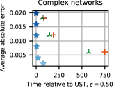
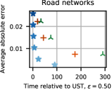
Figure 4: Arithmetic mean of the absolute errors $|\max_{v}\mathbf{\Omega}[v,v]-\widetilde{\mathbf{\Omega}}[v,v]|$ over the instances in Table 1.

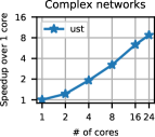
Figure 5: Geometric mean of the speedup of UST with $\varepsilon=\numprint{0.05}$ on multiple cores over a sequential run (shared memory). Data points are aggregated over the instances in Table 1.

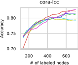
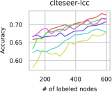
Figure 6: Accuracy in semi-supervised vertex classification on the largest connected component of the datasets when using different strategies to create the training set. Cora-lcc: $|V|=\numprint{2485},|E|=\numprint{5069}$, Citeseer-lcc: $|V|=\numprint{2110},|E|=\numprint{3668}$.

Complex networks

Graph	$|V|$	$|E|$	Time (s)
			$\varepsilon=0.1$	$\varepsilon=0.3$
soc-LiveJournal1	4,846,609	42,851,237	348.9	118.5
wikipedia_link_fr	3,333,397	100,461,905	205.4	90.7
orkut-links	3,072,441	117,184,899	293.5	92.2
dimacs10-uk-2002	18,483,186	261,787,258	1,101.3	365.8
wikipedia_link_en	13,593,032	334,591,525	919.3	295.4

Road networks

Graph	$|V|$	$|E|$	Time (s)
			$\varepsilon=0.1$	$\varepsilon=0.3$
slovakia	543,733	638,114	28.1	9.9
netherlands	1,437,177	1,737,377	82.9	31.1
greece	1,466,727	1,873,857	74.5	29.8
spain	4,557,386	5,905,365	273.0	86.2
great-britain	7,108,301	8,358,289	419.0	136.6
dach	20,207,259	25,398,909	1,430.1	473.7
africa	23,975,266	31,044,959	1,493.4	499.3

Table 2: Large networks used for scalability experiments in distributed memory and running time of UST on $16\times 24$ cores.

Graph	Group size	Time (s)
cora	200	1,559.3
	400	2,210.6
	600	2,663.4
citeseer	200	2,518.6
	400	3,666.5
	600	4,642.4

Table 3: Running time of our greedy algorithm for group forest maximization.

Complex networks

Graph	Time (s)
$\hfill\varepsilon$	$0.05$	$0.1$	$0.2$	$0.3$	$0.4$	$0.5$
loc-brightkite_edges	46.4	11.6	3.0	1.4	0.8	0.5
douban	80.8	20.5	5.2	2.4	1.5	0.9
soc-Epinions1	55.5	14.0	3.5	1.6	1.0	0.7
slashdot-zoo	59.9	15.6	3.8	1.8	1.1	0.7
petster-cat-household	61.8	15.7	4.0	1.8	1.1	0.8
wikipedia_link_fy	58.2	15.0	3.9	1.9	1.1	0.8
loc-gowalla_edges	230.9	63.0	15.7	7.1	4.4	2.8
wikipedia_link_an	50.7	12.1	3.1	1.5	0.9	0.7
wikipedia_link_ga	44.8	11.3	3.1	1.6	1.1	0.8
petster-dog-household	359.6	87.7	22.5	10.3	6.0	4.1
livemocha	107.4	28.6	7.3	3.5	2.1	1.5

Road networks

Graph	Time (s)
$\hfill\varepsilon$	$0.05$	$0.1$	$0.2$	$0.3$	$0.4$	$0.5$
mauritania	98.1	24.4	6.9	2.8	1.6	1.0
turkmenistan	118.5	30.2	7.7	3.4	2.1	1.3
cyprus	149.4	37.7	9.8	4.4	2.6	1.7
canary-islands	185.5	46.7	11.4	5.2	3.0	2.0
albania	192.6	52.6	13.1	6.0	3.4	2.2
benin	188.1	47.9	12.2	5.5	3.2	2.1
georgia	322.1	83.6	22.5	9.8	5.6	3.6
latvia	355.2	92.0	23.3	10.6	5.9	4.0
somalia	420.1	108.7	27.6	12.6	7.1	4.6
ethiopia	825.9	215.7	53.9	24.4	13.9	9.0
tunisia	1,200.1	303.1	77.7	34.6	19.7	12.9

Table 4: Running time in seconds of UST on the networks in Table 1.

References

- [1] E. Angriman, M. Predari, A. van der Grinten, and H. Meyerhenke. Approximation of the diagonal of a laplacian’s pseudoinverse for complex network analysis. In ESA, volume 173 of LIPIcs, pages 6:1–6:24. Schloss Dagstuhl - Leibniz-Zentrum für Informatik, 2020.
- [2] E. Angriman, A. van der Grinten, M. von Looz, H. Meyerhenke, M. Nöllenburg, M. Predari, and C. Tzovas. Guidelines for experimental algorithmics: A case study in network analysis. Algorithms, 12(7):127, 2019.
- [3] K. Avrachenkov, P. Gonçalves, and M. Sokol. On the choice of kernel and labelled data in semi-supervised learning methods. In WAW, volume 8305 of LNCS, pages 56–67. Springer, 2013.
- [4] A.-L. Barabási and Others. Network science. Cambridge university press, 2016.
- [5] S. Barthelmé, N. Tremblay, A. Gaudillière, L. Avena, and P.-O. Amblard. Estimating the inverse trace using random forests on graphs, 2019.
- [6] E. Bergamini, M. Wegner, D. Lukarski, and H. Meyerhenke. Estimating current-flow closeness centrality with a multigrid laplacian solver. In CSC, pages 1–12. SIAM, 2016.
- [7] P. Boldi and S. Vigna. Axioms for centrality. Internet Mathematics, 10(3-4):222–262, 2014.
- [8] B. Bollobás. Modern Graph Theory, volume 184 of Graduate Texts in Mathematics. Springer, 2002.
- [9] U. Brandes and D. Fleischer. Centrality measures based on current flow. In STACS, volume 3404 of LNCS, pages 533–544. Springer, 2005.
- [10] O. Chapelle, J. Weston, and B. Schölkopf. Cluster kernels for semi-supervised learning. In NIPS, pages 585–592. MIT Press, 2002.
- [11] P. Chebotarev and E. Shamis. On proximity measures for graph vertices. Automation and Remote Control, 59(10):1443–1459, 1998.
- [12] P. Chebotarev and E. Shamis. The matrix-forest theorem and measuring relations in small social groups, 2006.
- [13] P. Y. Chebotarev and E. Shamis. The forest metrics of a graph and their properties. AUTOMATION AND REMOTE CONTROL C/C OF AVTOMATIKA I TELEMEKHANIKA, 61(8; ISSU 2):1364–1373, 2000.
- [14] M. B. Cohen, R. Kyng, G. L. Miller, J. W. Pachocki, R. Peng, A. B. Rao, and S. C. Xu. Solving SDD linear systems in nearly mlogn time. In STOC, pages 343–352. ACM, 2014.
- [15] M. G. Everett and S. P. Borgatti. The centrality of groups and classes. The Journal of Mathematical Sociology, 23(3):181–201, 1999.
- [16] K. D. Gremban. Combinatorial Preconditioners for Sparse, Symmetric, Diagonally Dominant Linear Systems. PhD thesis, Carnegie Mellon University, October 1996. CMU CS Tech Report CMU-CS-96-123.
- [17] N. S. Izmailian, R. Kenna, and F. Y. Wu. The two-point resistance of a resistor network: a new formulation and application to the cobweb network. Journal of Physics A: Mathematical and Theoretical, 47(3):035003, 2013.
- [18] Y. Jin, Q. Bao, and Z. Zhang. Forest distance closeness centrality in disconnected graphs. In ICDM, pages 339–348. IEEE, 2019.
- [19] W. B. Johnson and J. Lindenstrauss. Extensions of lipschitz mappings into a hilbert space. Contemporary mathematics, 26(189-206):1, 1984.
- [20] J. Kunegis. KONECT: the koblenz network collection. In WWW (Companion Volume), pages 1343–1350. Intl. World Wide Web Conf. Steering Committee / ACM, 2013.
- [21] R. Kyng and S. Sachdeva. Approximate gaussian elimination for laplacians - fast, sparse, and simple. In FOCS, pages 573–582. IEEE Computer Society, 2016.
- [22] H. Li, R. Peng, L. Shan, Y. Yi, and Z. Zhang. Current flow group closeness centrality for complex networks? In WWW, pages 961–971. ACM, 2019.
- [23] R. Merris. Doubly stochastic graph matrices, ii. Linear and Multilinear Algebra, 45(2-3):275–285, 1998.
- [24] M. Newman. Networks. Oxford university press, 2018.
- [25] K. Okamoto, W. Chen, and X. Li. Ranking of closeness centrality for large-scale social networks. In FAW, volume 5059 of LNCS, pages 186–195. Springer, 2008.
- [26] R. A. Rossi and N. K. Ahmed. The network data repository with interactive graph analytics and visualization. In AAAI, 2015.
- [27] P. Sen, G. Namata, M. Bilgic, L. Getoor, B. Gallagher, and T. Eliassi-Rad. Collective classification in network data. AI Mag., 29(3):93–106, 2008.
- [28] O. Shchur, M. Mumme, A. Bojchevski, and S. Günnemann. Pitfalls of graph neural network evaluation. CoRR, abs/1811.05868, 2018.
- [29] C. L. Staudt, A. Sazonovs, and H. Meyerhenke. Networkit: A tool suite for large-scale complex network analysis. Network Science, 4(4):508–530, 2016.
- [30] A. S. Teixeira, P. T. Monteiro, J. A. Carriço, M. Ramirez, and A. P. Francisco. Spanning edge betweenness. In MLG, volume 24, pages 27–31, 2013.
- [31] P. Thomas. Semi-supervised learning by olivier chapelle, bernhard schölkopf, and alexander zien (review). IEEE Trans. Neural Networks, 20(3):542, 2009.
- [32] A. van der Grinten, E. Angriman, and H. Meyerhenke. Scaling up network centrality computations – a brief overview. it - Information Technology, 62:189 – 204, 2020.
- [33] S. White and P. Smyth. Algorithms for estimating relative importance in networks. In KDD, pages 266–275. ACM, 2003.
- [34] D. B. Wilson. Generating random spanning trees more quickly than the cover time. In STOC, pages 296–303. ACM, 1996.
- [35] D. Zhou, O. Bousquet, T. N. Lal, J. Weston, and B. Schölkopf. Learning with local and global consistency. In NIPS, pages 321–328. MIT Press, 2003.