Probabilistic Inference for Learning from Untrusted Sources

Abstract

Federated learning brings potential benefits of faster learning, better solutions, and a greater propensity to transfer when heterogeneous data from different parties increases diversity. However, because federated learning tasks tend to be large and complex, and training times non-negligible, it is important for the aggregation algorithm to be robust to non-IID data and corrupted parties. This robustness relies on the ability to identify, and appropriately weight, incompatible parties. Recent work assumes that a reference dataset is available through which to perform the identification. We consider settings where no such reference dataset is available; rather, the quality and suitability of the parties needs to be inferred. We do so by bringing ideas from crowdsourced predictions and collaborative filtering, where one must infer an unknown ground truth given proposals from participants with unknown quality. We propose novel federated learning aggregation algorithms based on Bayesian inference that adapt to the quality of the parties. Empirically, we show that the algorithms outperform standard and robust aggregation in federated learning on both synthetic and real data.

Introduction

For deep neural networks to address more complex tasks in the future it is likely that the participation of multiple users, and hence multiple sources of data, will need become more widespread. This practice has been widely used in object recognition Li and Deng (2019); Sohn et al. (2011); Li et al. (2016); Rahimpour et al. (2016); Paris et al. (2015), but less so in domains such as finance, medicine, prediction markets, internet of things, etc. Federated learning, as defined by McMahan et al. (2017b) is an answer to the problem of training complex, heterogeneous tasks. It involves distributing model training across a number of parties in a centralized manner while taking into account communication requirements, over potentially remote or mobile devices, privacy concerns requiring that data remains at the remote location, and the lack of balanced or IID data across parties.

One challenge in federated learning, as noted by Kairouz et al. (2019), is the quality and data distribution of the sources being used for the training tasks. A related challenge is the potential for random failures or adversarial parties to disrupt the federated training. For these reasons, robust federated learning has seen a flurry of activity Sattler et al. (2019); Bhagoji et al. (2019); Mohri, Sivek, and Suresh (2019); Ghosh et al. (2019); Pillutla, Kakade, and Harchaoui (2019b). Some, like Alistarh, Allen-Zhu, and Li (2018); Bhagoji et al. (2019); Xie, Koyejo, and Gupta (2018) focus on the adversarial setting, and others, like Konstantinov and Lampert (2019); Pillutla, Kakade, and Harchaoui (2019b), focus on the general setting of distributed learning under different source distributions. In both cases, this requires identifying the weight with which to include each party in the aggregation.

Konstantinov and Lampert (2019) proposed to give the aggregator a reference dataset with which to measure the quality of each party update. Like Konstantinov and Lampert (2019), we explore the question of efficient federated learning with unequal and possibly untrusted parties. However, the assumption of access to a reference dataset is, for many real-world problems, problematic. Consider a federation of medical diagnosis facilities, each with its own patient population. Not only would it violate privacy concerns to generate a reference dataset but it would not in fact be feasible. The same problem arises in virtually any real-world domain for which federated learning offers an appealing solution.

We propose instead to adapt inference methods from collaborative filtering Cai et al. (2020) to the problem of heterogeneous federated learning aggregation. Using a Gaussian model, we model each party’s estimate as a noisy observation of an unknown ground truth and define new probabilistic inference algorithms to iteratively estimate the ground truth. We show that the estimated ground truth is robust to faulty and poor quality data. Specifically, the contributions of this work are as follows:

• We provide a maximum likelihood estimator of the uncertainty level of each party in a federated learning training task. The estimator gives rise to an appropriate weighting for each party in each aggregation. When each party’s data sample is independent, the estimator reduces to the standard averaging scheme of McMahan et al. (2017a); in the more general case of overlapping samples, it offers a new maximum likelihood estimator.

• We define two new algorithms for federated learning that make use of the MLE: an inverse variance weighting and an inverse covariance weighting scheme.

• As the maximum likelihood estimator can overfit when the available data is scarce and tends to be computationally expensive for the inverse covariance scheme, we define a new Variational Bayesian (VB) approach to approximate the posterior distributions of the ground truth under both independent and latent noise models.

Both the MLE and VB methods are tested on synthetic and real datasets; the tests show the superiority of aggregation with probabilistic inference over standard baselines including the mean and the more robust median-based approaches: geometric median and coordinate-wise median.

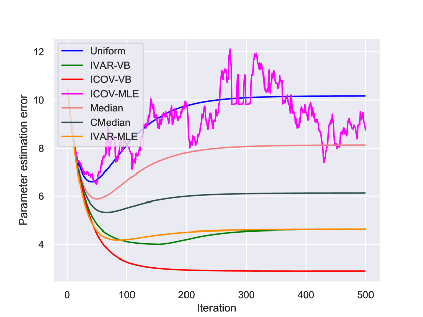
(a) Full participation. Full batch (300 samples)

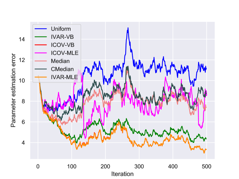
(b) Full participation. Mini batch (32 samples)

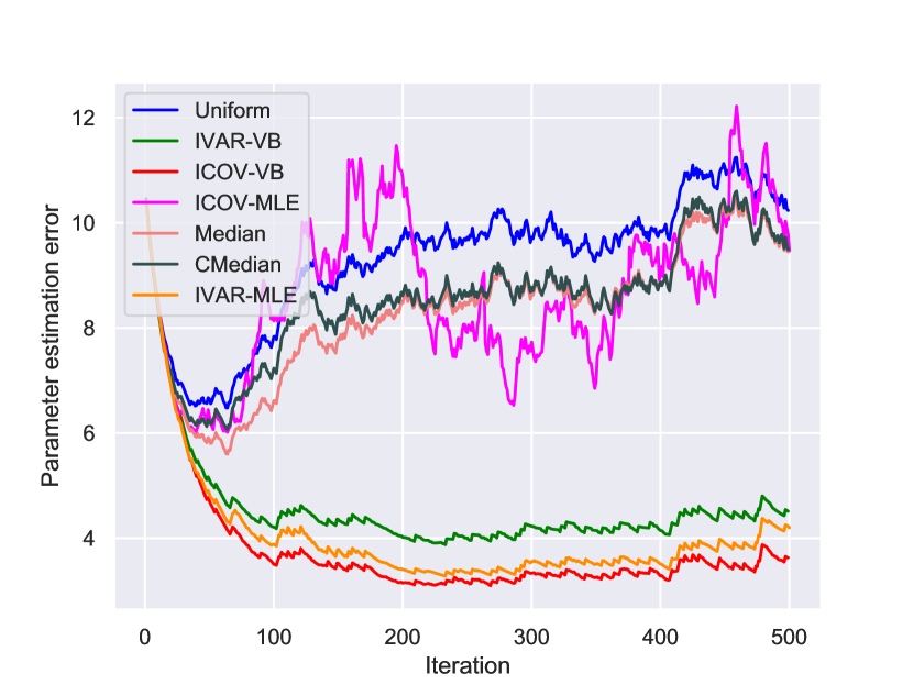
(c) Partial: 3 random parties per round. Full batch (300 samples)

Figure 1: Linear regression. ICOV and IVAR outperform other methods when there are adversaries.

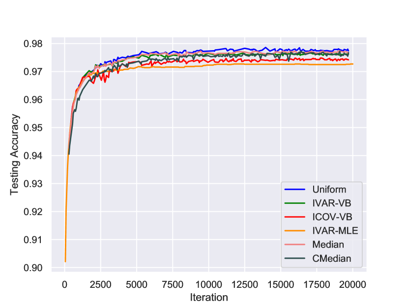
(a) 5 genuine parties, 0 adversaries

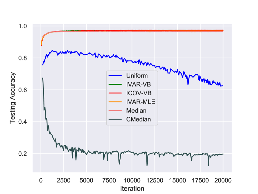
(b) 5 genuine parties, 5 adversaries

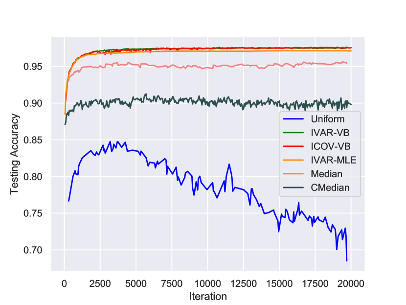
(c) 5 genuine parties, 10 adversar.

Figure 2: Adversarial MNIST testing performance. ICOV and IVAR outperform other methods with adversaries.

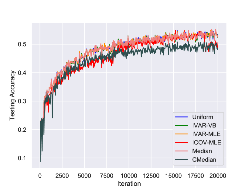
(a) 5 genuine parties, 0 adversaries

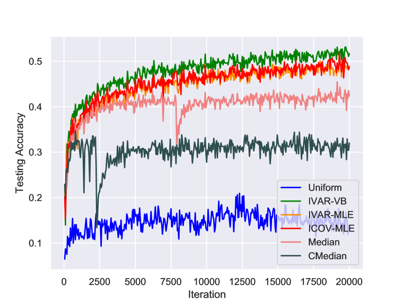
(b) 5 genuine parties, 5 adversaries

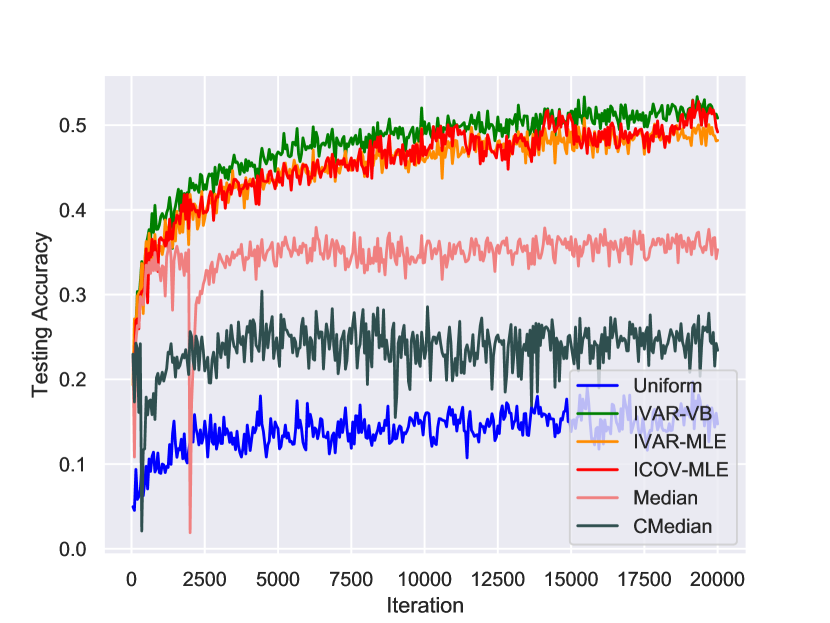
(c) 5 genuine parties, 10 adversar.

Figure 3: Adversarial Shakespeare testing performance. ICOV and IVAR outperform other methods with adversaries.

Related work

Robust Federated Learning

Konstantinov and Lampert (2019) propose a method for federated classification and regression using a reference dataset with which to weight the parties in the federation, in a manner similar to that of Song et al. (2018) for single-party, i.e. non-federated, training. They aggregate the parties using either the geometric median or the component-wise version thereof. Some methods such as Xie, Koyejo, and Gupta (2018) score the contribution of each party and then accept only those up to a threshold. Pillutla, Kakade, and Harchaoui (2019b) propose a stable variant of the geometric median algorithm for model parameter aggregation. The authors argue that parameter aggregation, as opposed to gradient aggregation, allows for more computation to occur on the devices and that assumptions on the distributions of parameters are easier to interpret. In our work we provide a mechanism to estimate the ground truth values for each party in a manner that applies to both gradients and model parameters.

A number of works such as Alistarh, Allen-Zhu, and Li (2018); Blanchard et al. (2017); Yin et al. (2018a); Bhagoji et al. (2019); Chen et al. (2018) study the byzantine setting with assumptions on the maximum number of adversarial parties, but do not in general consider the case of unbalanced data. Blanchard et al. (2017) propose a novel aggregation mechanism based on the distance of a party’s gradients to other gradients. Li et al. (2019) address the byzantine setting with non-iid data by penalizing the difference between local and global parameters, but do not consider unbalanced data. Chen et al. (2018) offer strong guarantees but under rather strong assumptions on the collusion of the parties, running contrary to most privacy requirements, and requiring significant redundancy with each party computing multiple gradients. Portnoy and Hendler (2020) are concerned with unbalanced data in a byzantine setting where parties erroneously report the sample size, and so propose to truncate weights reported by the parties to bound the impact of byzantine parties.

Collaborative Filtering

One of the earliest efforts in collaborative filtering was that of Dawid and Skene (1979) who proposed a Bayesian inference algorithm to aggregate individual worker labels and infer the ground truth in categorical labelling. Their approach defined the two main components of a collaborative filtering algorithm: estimating the reliability of each worker, and inferring the true label of each instance. They applied expectation maximization and estimated the ground truth in the E-step. Then, using the estimated ground truth, they compute the maximum likelihood estimates of the confusion matrix in the M-step. In continuous value labelling, Raykar et al. (2010) modeled each worker prediction as an independent noisy observation of the ground truth. Based on this independent noise assumption, Raykar et al. (2010) developed a counterpart to the Dawid-Skene framework for the continuous domain to infer both the unknown individual variance and the ground truth. In their M-step, the variance, which corresponds to the confusion matrix in categorical labelling, is computed to minimize the mean square error with respect to the estimated ground truth. Their E-step involves re-estimating the ground truth with a weighted sum of the individual predictions, where the weights are set as the inverses of individual variances. Liu, Peng, and Ihler (2012) point to the risk of convergence to a poor-quality local optimum of the above-mentioned EM approaches and propose a variational approach for the problem. Welinder et al. (2010) model each worker as a multi-dimensional quantity including bias and other factors, and group them as a function of those quantities. In federated learning, a party may also be considered to have a multidimensional set of attributes. In collaborative filtering, workers seldom participate in all of the tasks. This sparsity motivates the application of matrix factorization techniques. Federated learning also may exhibit this characteristic: if a party does not participate in all training rounds for reasons of latency, or suffers a failure, the result would be similar to the sparsity found in collaborative filtering. In continuous applications parties may exhibit correlations in their estimates. Li, Rubinstein, and Cohn (2019), in the context of crowdsourced classification, showed that the incorporation of cross-worker correlations significantly improves accuracy. That work relies on an extension of the (independent) Bayesian Classifier Combination model of Kim and Ghahramani (2012) in which worker correlation is modeled by representing true classes by mixtures of subtypes and motivates our inverse covariance scheme.

Problem Setup and Inference Models

Consider a global loss function

$$F(\mathbf{w})=\mathbb{E}_{\mathbf{z}}f(\mathbf{z};\mathbf{w})$$

where $\mathbf{w}$ is the parameter of interest and $\mathbb{E}$ denotes the expectation with respect to $\mathbf{z}\sim\mathcal{P}$ for some unknown distribution $\mathcal{P}$. In a federated learning setting, each worker party has access to samples from $\mathcal{P}$ and wish to jointly minimize $F(\mathbf{w})$ without revealing the local samples. Beginning with some initial $\mathbf{w}=\mathbf{w}_{0}$, learning happens over single or multiple rounds where each worker party submits a local update to a central aggregator. The local update can be in the form of model parameter $\mathbf{w}$ or gradient $\nabla_{\mathbf{w}}F(\mathbf{w})$.

Each round of such updates is considered a task; we use $i=1,\ldots,I$ to index such tasks. Workers are indexed by $j=1,\ldots,J$. We do not assume full participation in every update round, and use $J_{i}\subset\{1\ldots J\}$ to denote the set of participating workers for task $i$. Similarly, let $I_{j}\subset\{1\ldots I\}$ denote the set of tasks in which worker $j$ participates. Note that the term worker and party are synonymous, as both are used in the federated learning setting. In task $i$, each worker $j\in J_{i}$ sends an update $\mathbf{x}_{ij}$ to the aggregator. We make the following assumption regarding $\mathbf{x}_{ij}$:

Assumption 1.

The local update $\mathbf{x}_{ij}$ follows a Gaussian distribution $\mathbf{x}_{ij}\sim\mathcal{N}(\mathbf{y}_{i},\Sigma_{j})$.

We argue that the assumption is well-founded through the following examples.

Example 1.

Consider a learning scheme where each update to $\mathbf{w}$ computes an estimate of the global gradient $\nabla_{\mathbf{w}}F=\mathbb{E}_{\mathbf{z}}\nabla_{\mathbf{w}}f(\mathbf{z};\mathbf{w})$. Suppose that each worker $j$ has access to a sample $\mathcal{D}_{j}$ of independent examples from $\mathcal{P}$ and computes $\mathbf{x}_{ij}=\frac{1}{|\mathcal{D}_{j}|}\sum_{\mathbf{z}\in\mathcal{D}_{j}}\nabla_{\mathbf{w}}f(\mathbf{z};\mathbf{w})$. Let $\mathbf{y}_{i}=\mathbb{E}[\nabla_{\mathbf{w}}f(\mathbf{z};\mathbf{w})]$ and $\Sigma=\mathrm{Cov}[\nabla_{\mathbf{w}}f(\mathbf{z};\mathbf{w})]$. By the central limit theorem, as $|\mathcal{D}_{j}|\to\infty$, $\mathbf{x}_{ij}$ approches $\mathcal{N}(\mathbf{y}_{i},\Sigma_{j})$ in distribution, with $\Sigma_{j}=\frac{\Sigma}{|\mathcal{D}_{j}|}$.

Example 2.

Suppose that each local update is obtained by finding the maximum likelihood estimator for a linear model $\mathbf{z}_{j}=H_{j}\mathbf{y}_{i}+\mathbf{\epsilon}_{j}$ where $(H_{j},\mathbf{z}_{j})$ contains the observed local data. Assuming that $H_{j}$ is fixed while $\mathbf{\epsilon}_{j}$ follows a Gaussian distribution $\mathcal{N}(0,\sigma^{2}\mathbf{I})$, then the least-squares solution, given by $\mathbf{x}_{ij}=(H_{j}^{\top}H_{j})^{-1}H_{j}^{\top}\mathbf{z}_{j}$ also follows a Gaussian $\mathcal{N}(\mathbf{y}_{i},\Sigma_{j})$ where $\Sigma_{j}=\sigma^{2}(H_{j}^{\top}H_{j})^{-1}$.

Under Assumption 1, further suppose that each local sample is independent, the maximum likelihood estimator (MLE) for $\mathbf{y}_{i}$ is given by

$$\widehat{\mathbf{y}}_{i} =\arg\max_{\mathbf{y}}\sum_{j}-(\mathbf{x}_{ij}-\mathbf{y})^{\top}\Sigma_{j}^{-1}(\mathbf{x}_{ij}-\mathbf{y})$$

$$=\big{(}\sum_{j}\Sigma_{j}^{-1}\big{)}^{-1}\sum_{j}\Sigma_{j}^{-1}\mathbf{x}_{ij}.$$ (1)

In the case of Example 1, where $\Sigma_{j}=\frac{\Sigma}{|\mathcal{D}_{j}|}$, equation (Problem Setup and Inference Models) reduces to

$$\widehat{\mathbf{y}}_{i}=\frac{\sum_{j}|\mathcal{D}_{j}|\mathbf{x}_{ij}}{\sum_{j}|\mathcal{D}_{j}|}.$$ (2)

This justifies the standard averaging scheme in federated learning (McMahan et al., 2017a). Note that even under the Gaussian assumption, the standard averaging scheme is the MLE only when each worker has independent samples.

In general, if $\mathbf{x}_{ij}$ and $\mathbf{x}_{ij^{\prime}}$ are not independent, the MLE for $\mathbf{y}_{i}$ will be more complicated. Consider the simpler case where each component in $\mathbf{x}_{ij}$, denoted $x_{ij}^{k}$ for $k=1\ldots K$, is independent across $k$, fixing $i,j$. On the other hand, they may be correlated among the workers, i.e. across $j$ fixing $i,k$. Assumption 1 specializes to:

Assumption 2.

The local update $\mathbf{x}_{ij}$ follows a Gaussian distribution $\mathbf{x}_{ij}\sim\mathcal{N}(\mathbf{y}_{i},\sigma_{j}^{2}\mathbf{I})$. Furthermore, let $\Phi$ be a $J\times J$ covariance matrix where $\Phi_{j,j}=\sigma_{j}^{2}$ and $\Phi_{j,j^{\prime}}=\mathrm{Cov}(x_{ij}^{k},x_{ij^{\prime}}^{k})$ for all $k$ and $j\neq j^{\prime}$. The vector $\mathbf{x}_{i,:}^{k}=[x_{i1}^{k}\ldots x_{iJ}^{k}]^{\top}$ follows a Gaussian distribution $\mathbf{x}_{i,:}^{k}\sim\mathcal{N}(y_{i}^{k}\mathbf{1},\Phi)$.

The MLE for $\mathbf{y}_{i}$ and $\Phi$ under this setting is given by:

Proposition 1.

Under Assumption 2, let $X_{i,\mathbf{j}_{i}}$ be the matrix whose columns are $\mathbf{x}_{ij}$ for participating workers $j\in J_{i}$ and $\Phi_{\mathbf{j}_{i}}$ the corresponding submatrix of $\Phi$. The MLE for $\mathbf{y}_{i}$ (fixing $\Phi_{\mathbf{j}_{i}}$) and $\Phi_{\mathbf{j}_{i}}$ (fixing $\mathbf{y}_{i}$) are given, respectively, by

$$\widehat{\mathbf{y}}_{i}=\frac{X_{i,\mathbf{j}_{i}}\Phi_{\mathbf{j}_{i}}^{-1}\mathbf{1}}{\mathbf{1}^{\top}\Phi_{\mathbf{j}_{i}}^{-1}\mathbf{1}}$$ (3)

and

$$\widehat{\Phi}_{\mathbf{j}_{i}}=\frac{1}{K}(X_{i,\mathbf{j}_{i}}-\mathbf{y}_{i}\mathbf{1}^{\top})^{\top}(X_{i,\mathbf{j}_{i}}-\mathbf{y}_{i}\mathbf{1}^{\top}).$$ (4)

Proof.

Let $\mathbf{x}_{i,\mathbf{j}_{i}}^{k}$ be the (column) vector corresponds to the $k$-th row of $X_{i,\mathbf{j}_{i}}$. Under Assumption 2, we have that $\mathbf{x}_{i,\mathbf{j}_{i}}^{k}\sim\mathcal{N}(y_{i}^{k}\mathbf{1},\Phi_{\mathbf{j}_{i}})$. The log-likelihood for $\mathbf{x}_{i,\mathbf{j}_{i}}^{k}$ is given by

$$\log p(\mathbf{x}_{i,\mathbf{j}_{i}}^{k}|y_{i}^{k},\Phi_{\mathbf{j}_{i}})$$

$$= \frac{1}{2}\log|\Phi_{\mathbf{j}_{i}}^{-1}|-\frac{1}{2}(\mathbf{x}_{i,\mathbf{j}_{i}}^{k}-y_{i}^{k}\mathbf{1})^{\top}\Phi_{\mathbf{j}_{i}}^{-1}(\mathbf{x}_{i,\mathbf{j}_{i}}^{k}-y_{i}^{k}\mathbf{1})+c$$

for $c$ constant. The MLE can be obtained by computing $\frac{\partial}{\partial y_{i}^{k}}\log p(\mathbf{x}_{i,\mathbf{j}_{i}}^{k}|y_{i}^{k},\Phi_{\mathbf{j}_{i}})$ and $\frac{\partial}{\partial(\Phi_{\mathbf{j}_{i}}^{-1})}\log p(\mathbf{x}_{i,\mathbf{j}_{i}}^{k}|y_{i}^{k},\Phi_{\mathbf{j}_{i}})$ respectively and finding the stationary points. ∎

Remark 1.

Note that under Assumption 2, $\Phi$ is shared by all tasks $i=1\ldots I$. Equation (4) can therefore be extended to use the data across multiple tasks, resulting in the following update for all $j,j^{\prime}$:

$$\widehat{\Phi}_{j,j^{\prime}}=\frac{1}{K|I_{j}\cap I_{j^{\prime}}|}\sum_{i\in I_{j}\cap I_{j^{\prime}}}(\mathbf{x}_{ij}-\mathbf{y}_{i})^{\top}(\mathbf{x}_{ij^{\prime}}-\mathbf{y}_{i}).$$

Let us go back to Example 1 where each local update $\mathbf{x}_{ij}$ is the average of independent examples from $\mathcal{D}_{j}$ but for any two workers $j\neq j^{\prime}$, $\mathcal{D}_{j}$ and $\mathcal{D}_{j^{\prime}}$ can overlap. We have:

Proposition 2.

Under Assumption 2, let $\mathbf{x}_{ij}=\frac{1}{|\mathcal{D}_{j}|}\sum_{\mathbf{g}\in\mathcal{D}_{j}}\mathbf{g}$ where $\mathbf{g}\sim\mathcal{N}(\mathbf{y}_{i},\sigma^{2}\mathbf{I})$. Assume that for each $j$, all $\mathbf{g}\in\mathcal{D}_{j}$ are independent, but $\mathcal{D}_{j}\cap\mathcal{D}_{j^{\prime}}$ may be non-empty for any $j\neq j^{\prime}$. Then

$$\Phi_{j,j^{\prime}}=\frac{|\mathcal{D}_{j}\cap\mathcal{D}_{j^{\prime}}|}{|\mathcal{D}_{j}||\mathcal{D}_{j^{\prime}}|}\sigma^{2}.$$ (5)

Proof.

Fix a component $k$ of $\mathbf{g}$, we have that $g^{k}\sim\mathcal{N}(y_{i}^{k},\sigma^{2})$. Let $|\mathcal{D}_{j}|=n_{1}+m$, $|\mathcal{D}_{j^{\prime}}|=n_{2}+m$ and $n=n_{1}+n_{2}+m$. Draw $n$ independent examples $g^{k}_{1}\ldots g^{k}_{n}$ from $\mathcal{N}(y_{i}^{k},\sigma^{2})$ such that $\mathcal{D}_{j}^{k}=\{g^{k}_{1}\ldots g^{k}_{n_{1}},g^{k}_{n_{1}+n_{2}+1}\ldots g^{k}_{n_{1}+n_{2}+m}\}$ and $\mathcal{D}_{j^{\prime}}^{k}=\{g^{k}_{n_{1}+1}\ldots g^{k}_{n_{1}+n_{2}},g^{k}_{n_{1}+n_{2}+1}\ldots g^{k}_{n_{1}+n_{2}+m}\}$. Note that $m$ is the number of overlapping examples.

Let $\mathbf{x}=[g^{k}_{1}\ldots g^{k}_{n}]^{\top}$ and choose $A$ such that $A\mathbf{x}=[x_{ij}^{k},x_{ij^{\prime}}^{k}]^{\top}$. We use the fact that for a constant matrix $A$ and random vector $\mathbf{x}$, $\mathrm{Cov}(A\mathbf{x})=A\mathrm{Cov}(\mathbf{x})A^{\top}$. Note that $\mathrm{Cov}(\mathbf{x})=\sigma^{2}\mathbf{I}$. The result then follows by inspecting the entries in $A\mathrm{Cov}(\mathbf{x})A^{\top}$. ∎

With overlapping local samples, one can solve the MLE of $\mathbf{y}_{i}$ using Equation (3) with $\Phi$ from Equation (5). If there is no overlap, then we again obtain (2). In practice, however, it is unlikely that the aggregator has access to the sample size as well as the sample overlap between any workers. Our proposed approach is therefore to jointly estimate both $\mathbf{y}_{i}$ and the unknown $\Phi$ under Assumption 2. We present in what follows two new methods for doing so. In the first we suppose that $\Phi$ is diagonal; this results in an Inverse Variance Weighting method, called IVAR. In the second we estimate the full covariance matrix, $\Phi$, in what we term Inverse Covariance Weighting, or ICOV.

Inverse Variance Weighting

Inverse variance weighting has been used in collaborative filtering for aggregation without a ground truth. Inverse variance weighting has an appealing interpretation as the maximum-likelihood estimation under a bias-variance model, based on the assumption that parties have independent additive prediction noise  Liu, Ihler, and Steyvers (2013); Raykar et al. (2010); Kara et al. (2015). As such, the Gaussian model of Assumption 2 is a good approximation.

We adapt this idea to federated learning as follows. Let the ground truth be $\mathbf{y}_{i}$ for each $i$. Learning the full covariance matrix $\Phi$ can be expensive if the number of parties $J$ is large. This justifies developing a method that uses a diagonal matrix with $\Phi_{j,j^{\prime}}=0$ for $j\neq j^{\prime}$. Then, the maximum likelihood aggregation can be computed as follows:

Proposition 3.

Under Assumption 2, let $\Phi$ be diagonal. The MLE for $\mathbf{y}_{i}$ (fixing $\Phi$) is given by

$$\widehat{\mathbf{y}}_{i}=\frac{\sum_{j\in J_{i}}(1/\sigma^{2}_{j})\mathbf{x}_{ij}}{\sum_{j\in J_{i}}1/\sigma^{2}_{j}}.$$ (6)

For each $j$, the MLE for $\sigma_{j}^{2}$ (fixing $\mathbf{y}_{i}$) is given by

$$\widehat{\sigma}_{j}^{2}=\frac{1}{K}\|\mathbf{x}_{ij}-\mathbf{y}_{i}\|^{2}$$ (7)

where $\|\cdot\|$ is the Euclidean norm.

Proof.

The results follow from Proposition 1. ∎

The MLE for $\mathbf{y}_{i}$ and $\sigma_{j}^{2}$ can be jointly optimized by iterating on Equations (6) and (7). In particular, beginning with $\widehat{\mathbf{y}}_{i}^{(0)}$, each update is given by:

$$\widehat{\mathbf{y}}_{i}^{(t+1)}=\frac{\sum_{j\in J_{i}}\big{(}1/\|\mathbf{x}_{ij}-\widehat{\mathbf{y}}_{i}^{(t)}\|^{2}\big{)}\mathbf{x}_{ij}}{\sum_{j\in J_{i}}\big{(}1/\|\mathbf{x}_{ij}-\widehat{\mathbf{y}}_{i}^{(t)}\|^{2}\big{)}}.$$

This bears a resemblance to Weiszfeld’s algorithm to estimate the geometric median Pillutla, Kakade, and Harchaoui (2019a), where each update is given by:

$$\widehat{\mathbf{y}}_{i}^{(t+1)}=\frac{\sum_{j\in J_{i}}\big{(}1/\|\mathbf{x}_{ij}-\widehat{\mathbf{y}}_{i}^{(t)}\|\big{)}\mathbf{x}_{ij}}{\sum_{j\in J_{i}}\big{(}1/\|\mathbf{x}_{ij}-\widehat{\mathbf{y}}_{i}^{(t)}\|\big{)}}.$$

Input: $\langle\sigma_{j},\mathbf{x}_{ij}\rangle_{i\in\tilde{I},j\in\mathbf{J}_{i}}$

1 for $t\rightarrow 1:T$ do

2       $\mathbf{y}^{(t)}_{i}\leftarrow\frac{\sum_{j\in\mathbf{j}_{i}}1/\sigma^{2}_{j}\mathbf{x}_{ij}}{\sum_{j\in\mathbf{j}_{i}}1/\sigma^{2}_{j}},\forall i\in\tilde{I}$

3       $\sigma^{2}_{j}\leftarrow\max\{\epsilon,(1/(K|\tilde{I}_{j})|)\sum_{i\in\tilde{I}_{j}}\|\mathbf{y}^{(t)}_{i}-\mathbf{x}_{ij}\|^{2}_{2}\}$, $\forall j$

4      

Output: $\mathbf{y}^{(T)}_{i},\langle\sigma_{j}\rangle_{j\in\mathbf{j}_{i}}$

Algorithm 1 Inverse-Variance Weighting Aggregator

The algorithm for inverse variance weight aggregation, IVAR, provided in Algorithm 1, works as follows: upon receiving the local update for tasks $\tilde{I}$, the aggregator iteratively computes the “consensus” $\mathbf{y}^{(t)}_{i}$ for each task $i$ using the variance $\sigma_{j}$ of each worker $j$. Note that, as $\sigma_{j}$ is assumed invariant over tasks, it can be computed as the average variance.

Inverse Covariance Weighting

The independence assumption in the bias-variance model can be violated in federated learning scenarios when parties use similar information and methods. This gives rise to a collective bias within groups of parties. Ideally one would like then to estimate the full covariance matrix $\Phi$, such as using iterative updates from Proposition 1. The number of parameters grows with $J^{2}$ however and may give poor estimations if groups do not jointly participate in many of the tasks. This motivates the use of a latent feature model that allows for noise correlation across parties while addressing the challenge of sparse observations. In particular, consider the following probabilistic model for each local update. Without loss of generality, let $K=1$ and omit index $k$:

$$x_{ij}\sim\mathcal{N}\left(y_{i}+\mathbf{u}_{i}^{\top}\mathbf{v}_{j},\sigma^{2}\right),$$ (8)

where $\mathbf{u}_{i}\in R^{D}$ and $\mathbf{v}_{j}\in R^{D}$ are latent feature vectors associated with task $i$ and worker $j$, respectively. As such, all observations are correlated by the unknown latent feature vectors. Let $X$ be the local updates over multiple tasks with entries $X_{ij}=x_{ij}$. Consider maximizing the log-likelihood:

$$\log p\left(\mathbf{X}\left|\mathbf{y},\mathbf{U},\mathbf{V},\sigma^{2}\right.\right)$$

$$= \sum_{(i,j):i\in I_{j}}\log p\left(x_{ij}\left|y_{i},\mathbf{u}_{i},\mathbf{v}_{j},\sigma^{2}\right.\right),$$

where matrices $\mathbf{U}\coloneqq\left[\mathbf{u}_{1},\dots,\mathbf{u}_{I}\right]^{\top}\in R^{I\times D}$ and $\mathbf{V}\coloneqq\left[\mathbf{v}_{1},\dots,\mathbf{v}_{J}\right]^{\top}\in R^{J\times D}$. In particular, we extend inverse covariance weighting by a nonlinear matrix factorization technique based on Gaussian processes Lawrence and Urtasun (2009) to jointly infer the ground truth and the latent feature vectors. From (8), observe that, by placing independent zero mean Gaussian priors $\mathcal{N}(\mathbf{0},\sigma_{u}^{2}\mathbf{I})$ on $\mathbf{u}_{i}$, we recover the probabilistic model of Assumption 2 where $\mathbf{x}_{i,:}\sim\mathcal{N}(y_{i}\mathbf{1},\Phi)$ with the covariance matrix:

$$\Phi=\sigma_{u}^{2}\mathbf{V}\mathbf{V}^{\top}+\sigma^{2}\mathbf{I}.$$

Thus, the problem of covariance estimation has been transformed into the problem of estimating $\mathbf{V}$, $\sigma_{u}^{2}$, $\sigma^{2}$. The degrees of freedom are now determined by the size of $\mathbf{V}$ which contains $J\times D$ values. Since we expect $D\ll J$ in practical applications, this problem has significantly fewer degrees of freedom than the original problem of estimating the $J^{2}$ values of the entire covariance matrix.

Maximizing the log-likelihood involves alternating between the optimization of $\mathbf{y}$ and $(\mathbf{V},\sigma^{2},\sigma_{u}^{2})$. Specifically, update $\mathbf{y}$ using equation (3) and perform stochastic gradient descent on the model parameters as there is no closed-form solution for the latter. The log-likelihood for round $i$ is:

$$E_{i}(\mathbf{V},\sigma^{2},\sigma_{u}^{2})=-\log\left|\Phi_{\mathbf{j}_{i}}\right|-\boldsymbol{\delta}_{i,\mathbf{j}_{i}}^{\top}\Phi_{\mathbf{j}_{i}}^{-1}\boldsymbol{\delta}_{i,\mathbf{j}_{i}}+\text{const.}$$

and the gradients with respect to the parameters are:

$$\nabla_{\mathbf{V}_{\mathbf{j}_{i},:}}E_{i}(\mathbf{V},\sigma^{2},\sigma_{u}^{2}) =2\sigma_{u}^{2}\mathbf{G}_{i}\mathbf{V}_{\mathbf{j}_{i},:},$$ (9a)

$$\nabla_{\sigma^{2}}E_{i}(\mathbf{V},\sigma^{2},\sigma_{u}^{2}) =\mathrm{Tr}\left(\mathbf{G}_{i}\right),$$ (9b)

$$\nabla_{\sigma_{u}^{2}}E_{i}(\mathbf{V},\sigma^{2},\sigma_{u}^{2}) =\mathrm{Tr}\left(\mathbf{G}_{i}\mathbf{V}_{\mathbf{j}_{i},:}\mathbf{V}_{\mathbf{j}_{i},:}^{\top}\right).$$ (9c)

where $\boldsymbol{\delta}_{i,\mathbf{j}_{i}}=(\mathbf{x}_{i,\mathbf{j}_{i}}-y_{i}\mathbf{1})$, $\mathbf{G}_{i}\coloneqq\Phi_{\mathbf{j}_{i}}^{-1}\boldsymbol{\delta}_{i,\mathbf{j}_{i}}\boldsymbol{\delta}_{i,\mathbf{j}_{i}}^{\top}\Phi_{\mathbf{j}_{i}}^{-1}-\Phi_{\mathbf{j}_{i}}^{-1}$ and $\mathbf{V}_{\mathbf{j}_{i},:}\in R^{|J_{i}|\times D}$ is the submatrix of $\mathbf{V}$ containing the rows corresponding to the indices in $J_{i}$. After inferring the covariance matrix, computing the ground truth for new instances can be done with Eq. (3). One can also model the covariance matrix with non-linear kernel functions by replacing the inner products $\mathbf{v}_{j}^{\top}\mathbf{v}_{j^{\prime}}$ in the covariance expression by a Mercer kernel function $k(\mathbf{v}_{j},\mathbf{v}_{j^{\prime}})$. The parameters in the kernel representation can be optimized by gradient descent on the log-likelihood function. We focus, however, on the linear kernel $k(\mathbf{v}_{j},\mathbf{v}_{j^{\prime}})=\mathbf{v}_{j}^{\top}\mathbf{v}_{j^{\prime}}$.

Variational Bayesian (VB) Inference

The maximum-likelihood estimator can lead to overfitting when the available data is scarce, and gradient updates  (9a)-(9c) for inverse covariance weighting are computationally expensive. For improved robustness and computational efficiency, we propose a Variational Bayesian approach to approximate the posterior distributions of the ground truth under both independent and latent noise models.

Independent Noise Model

Under Assumption 2, we place a prior over the ground truth $y_{i}$ for each $i$. Again, assume $K=1$ without loss of generality. Consider the simplest prior: a zero-mean Gaussian $y_{i}\sim\mathcal{N}(0,\tau^{2})$ where $\tau^{2}$ is a hyperparameter, though this can be extended to non-zero-mean priors. From the observed data $\mathbf{X}$, estimate the full posterior $p(\mathbf{y}|\mathbf{X})$ instead of a point estimate $\widehat{\mathbf{y}}$. The variational approximate inference procedure approximates the posterior $p(\mathbf{y}|\mathbf{X})$ by finding the distribution $q_{y}$ that maximizes the (negative of the) variational free energy:

$$F\left(q_{y}\right)=\mathbb{E}_{q_{y}}\left[\log\frac{p\left(\mathbf{X},\mathbf{y}\right)}{q_{y}(\mathbf{y})}\right],$$

where the joint probability is given by:

$$p\left(\mathbf{X},\mathbf{y}\right)=\prod_{(i,j):i\in I_{j}}p\left(x_{ij}\left|y_{i}\right.\right)\prod_{i}p\left(y_{i}\right).$$

Setting the derivative of $F$ w.r.t $q_{y}$ to zero implies that the stationary distributions are independent Gaussians:

$$q_{y}\left(\mathbf{y}\right)=\prod_{i}\mathcal{N}\left(y_{i}\left|\bar{y}_{i},\lambda_{i}\right.\right).$$

where means and covariances satisfy the following:

$$\lambda_{i} =\left(\frac{1}{\tau^{2}}+\sum_{j\in J_{i}}\frac{1}{\sigma_{j}^{2}}\right)^{-1},$$ (10)

$$\bar{y}_{i} =\lambda_{i}\sum_{j\in J_{i}}\frac{x_{ij}}{\sigma_{j}^{2}}.$$ (11)

In this case, Eq. (10) and (11) provide the exact posterior for the ground truth $\mathbf{y}$ given $\mathbf{X}$. Updating the hyperparameters by minimizing the variational free energy results in:

$$\tau^{2} =\frac{1}{I}\sum_{i}\lambda_{i}+\bar{y}_{i}^{2},$$ (12)

$$\sigma_{j}^{2} =\frac{1}{|I_{j}|}\sum_{i\in I_{j}}\left(\lambda_{i}+\left(x_{ij}-\bar{y}_{i}\right)^{2}\right).$$ (13)

In summary, the proposed approach performs block coordinate descent by applying repeatedly eq. (10) to (13) and aggregates using the posterior mean $\bar{y}_{i}$.

Latent Noise Model

One of the key steps in the MLE approach to Inverse Covariance Weighting is the marginalization of $\mathbf{U}$ conditioned on $(\mathbf{V},\sigma^{2},\sigma_{u}^{2})$. This can be interpreted as Bayesian averaging over $\mathbf{U}$. However, full Bayesian averaging over both $\mathbf{U}$ and $\mathbf{V}$ is challenging, motivating the Variational Bayes approach. First, place zero mean Gaussian priors on the latent variables:

$$p\left(y_{i},\sigma_{y}^{2}\right)=\mathcal{N}\left(y_{i}\left|0,\sigma_{y}^{2}\right.\right),$$

$$p\left(\mathbf{u}_{i},\sigma_{u}^{2}\right)=\mathcal{N}\left(\mathbf{u}_{i}\left|\mathbf{0},\sigma_{u}^{2}\mathbf{I}\right.\right),$$

$$p\left(\mathbf{v}_{j},\sigma_{v}^{2}\right)=\mathcal{N}\left(\mathbf{v}_{j}\left|\mathbf{0},\sigma_{v}^{2}\mathbf{I}\right.\right),$$

where $\sigma_{y}^{2}$, $\sigma_{u}^{2}$, $\sigma_{v}^{2}$ are hyperparameters. For notational brevity, we omit the dependence of the distributions on the hyperparameters $\sigma^{2}$, $\sigma_{y}^{2}$, $\sigma_{u}^{2}$, $\sigma_{v}^{2}$. The variational inference procedure finds distributions that maximize the (negative of the) variational free energy of the model from (8), assuming a factored distribution $q(\mathbf{y},\mathbf{U},\mathbf{V})=q_{y}(\mathbf{y})q_{u}(\mathbf{U})q_{v}(\mathbf{V})$:

$$F\left(q_{y},q_{u},q_{v}\right)=\mathbb{E}_{q_{y},q_{u},q_{v}}\left[\log\frac{p\left(\mathbf{X},\mathbf{y},\mathbf{U},\mathbf{V}\right)}{q_{y}(\mathbf{y})q_{u}(\mathbf{U})q_{v}(\mathbf{V})}\right],$$

where the joint probability is:

$$p\left(\mathbf{X},\mathbf{y},\mathbf{U},\mathbf{V}\right) =\prod_{(i,j):i\in I_{j}}p\left(x_{ij}\left|y_{i},\mathbf{u}_{i},\mathbf{v}_{j}\right.\right)$$

$$\qquad\;\times\prod_{i}p\left(y_{i}\right)\prod_{i}p\left(\mathbf{u}_{i}\right)\prod_{j}p\left(\mathbf{v}_{j}\right).$$

Then, solve for $q_{y}$, $q_{u}$ and $q_{v}$ by performing block coordinate descent on $F$. The resulting posterior distributions are Gaussians where $q_{y}(\mathbf{y})=\prod_{i}\mathcal{N}(y_{i}|\bar{y}_{i},\lambda_{i})$, $q_{u}(\mathbf{U})=\prod_{i}\mathcal{N}(\mathbf{u}_{i}|\bar{\mathbf{u}}_{i},\Phi_{i})$, and $q_{v}(\mathbf{V})=\prod_{j}\mathcal{N}(\mathbf{v}_{j}|\bar{\mathbf{v}}_{j},\Psi_{j})$. The means and covariances are given by:

$$\lambda_{i} =\left(\frac{1}{\sigma_{y}^{2}}+\sum_{j\in J_{i}}\frac{1}{\sigma^{2}}\right)^{-1},$$ (14)

$$\bar{y}_{i} =\lambda_{i}\sum_{j\in J_{i}}\frac{1}{\sigma^{2}}\left(x_{ij}-\bar{\mathbf{u}}_{i}^{\top}\bar{\mathbf{v}}_{j}\right),$$ (15)

$$\boldsymbol{\Phi}_{i} =\left(\frac{1}{\sigma_{u}^{2}}\mathbf{I}+\sum_{j\in J_{i}}\frac{1}{\sigma^{2}}\left(\boldsymbol{\Psi}_{j}+\bar{\mathbf{v}}_{j}\bar{\mathbf{v}}_{j}^{\top}\right)\right)^{-1},$$ (16)

$$\bar{\mathbf{u}}_{i} =\boldsymbol{\Phi}_{i}\sum_{j\in J_{i}}\frac{1}{\sigma^{2}}\left(x_{ij}-\bar{y}_{i}\right)\bar{\mathbf{v}}_{j},$$ (17)

$$\boldsymbol{\Psi}_{j} =\left(\frac{1}{\sigma_{v}^{2}}\mathbf{I}+\sum_{i\in I_{j}}\frac{1}{\sigma^{2}}\left(\boldsymbol{\Phi}_{i}+\bar{\mathbf{u}}_{i}\bar{\mathbf{u}}_{i}^{\top}\right)\right)^{-1},$$ (18)

$$\bar{\mathbf{v}}_{j} =\boldsymbol{\Psi}_{j}\sum_{i\in I_{j}}\frac{1}{\sigma^{2}}\left(x_{ij}-\bar{y}_{i}\right)\bar{\mathbf{u}}_{i}.$$ (19)

The hyperparameter updates are given by:

$$\sigma_{y}^{2} =\frac{1}{I}\left(\sum_{i}\left(\lambda_{i}+\bar{y}_{i}^{2}\right)\right),$$ (20)

$$\sigma_{u}^{2} =\frac{1}{DI}\left(\sum_{i}\mathrm{Tr}\left(\boldsymbol{\Phi}_{i}+\bar{\mathbf{u}}_{i}\bar{\mathbf{u}}_{i}^{\top}\right)\right),$$ (21)

$$\sigma_{v}^{2} =\frac{1}{DJ}\left(\sum_{j}\mathrm{Tr}\left(\boldsymbol{\Psi}_{j}+\bar{\mathbf{v}}_{j}\bar{\mathbf{v}}_{j}^{\top}\right)\right),$$ (22)

$$\sigma^{2} =\frac{1}{\sum_{j}|I_{j}|}\sum_{(i,j):i\in I_{j}}\left[\lambda_{i}+\left(x_{ij}-\bar{y}_{i}\right)^{2}-2\left(x_{ij}-\bar{y}_{i}\right)\bar{\mathbf{u}}_{i}^{\top}\bar{\mathbf{v}}_{j}\right.$$

$$\qquad\qquad\quad\;+\mathrm{Tr}\left(\left(\boldsymbol{\Psi}_{i}+\bar{\mathbf{u}}_{i}\bar{\mathbf{u}}_{i}^{\top}\right)\left(\boldsymbol{\Phi}_{j}+\bar{\mathbf{v}}_{j}\bar{\mathbf{v}}_{j}^{\top}\right)\right)\Big{]}.$$ (23)

In summary, the algorithm applies equations (14) to (23) repeatedly until convergence.

Input: $\langle\mathbf{v}_{j},\sigma_{j},\mathbf{x}_{ij}\rangle_{j\in\mathbf{j}_{i}}$

1 for $t\rightarrow 1:T$ do

2       $\boldsymbol{\Sigma}_{\mathbf{j}_{i}}=\sigma_{u}^{2}\mathbf{V}_{\mathbf{j}_{i}}\mathbf{V}_{\mathbf{j}_{i}}^{\top}+\textbf{diag}(\sigma^{2}_{\mathbf{j}_{i}})$

3       $y^{(t)}_{i}=\frac{\mathbf{1}^{\top}{\boldsymbol{\Sigma}}_{\mathbf{j}_{i}}^{-1}x_{i,\mathbf{j}_{i}}}{\mathbf{1}^{\top}{\boldsymbol{\Sigma}}_{\mathbf{j}_{i}}^{-1}\mathbf{1}}$

4       Update using  (14)-(23).

Output: $\mathbf{y}^{(T)}_{i},\langle\mathbf{v}_{j},\sigma_{j},\mathbf{x}_{ij}\rangle_{j\in\mathbf{j}_{i}}$

Algorithm 2 Inverse Covariance Weighting Aggregator

	Synthetic	MNIST	Shakespeare
Uniform avg.	10.17	0.4926	0.16
Geom. media	8.13	0.5233	0.41
Coord. median	6.131	0.7987	0.29
IVAR-VB	4.62	0.8943	0.56
IVAR-MLE	4.66	0.9043	0.50
ICOV-VB	2.89	0.8932	0.52
ICOV-MLE	8.75	0.5253	N.A

Table 1: Performance of the federated learning aggregation algorithms, uniform averaging, geometric median, and coordinate-wise median, against proposed IVAR and ICOV, MLE and VB versions. In the Synthetic linear regression example, with full participation of 5 genuine parties and full batch, prediction error is shown, hence lower is better. On the one-round MNIST task and 5 genuine parties and 5 adversaries, prediction accuracy is shown, so higher is better. In the multi-round stochastic gradient aggregation task using the Shakespeare dataset, with 5 genuine parties and 5 adversaries accuracy is provided so again higher is better.

Experiments

We present experimental results with a synthetic dataset and two real datasets: MNIST and Shakespeare McMahan et al. (2017a). We compare (1) Uniform averaging (2) Geometric median which uses the smoothed Weiszfeld algorithm of Pillutla, Kakade, and Harchaoui (2019a) (3) Coordinate-wise median which uses the coordinate-wise median as in Yin et al. (2018b) (4) our proposed IVAR, using the MLE formulation and using the VB (5) our proposed ICOV, again using the MLE formulation and using VB, which computes a low-rank estimation of the covariance matrix.

Synthetic dataset experiment

We design a synthetic linear regression experiment to create an environment where each party in the federation has a different noise level, and the local data of each party is overlapping. The experimental setup is provided in the Supplementary Materials. Figure 1 shows the algorithm performance for various levels of participation and batch size. ICOV performs better than IVAR, and both ICOV and IVAR outperform the other baselines.

MNIST

In this adversarial MNIST classification task, a Gaussian adversary submits a random vector with components generated from a standard normal, $\mathcal{N}(0,1)$. We first study one-round parameter estimation using using logistic regression, as in Yin et al. (2018b) with 5 genuine parties and $R\in[0,10]$ adversaries. Bayesian inference aggregation IVAR and ICOV outperform the other algorithms including robust estimators coordinate-wise median and geometric median when the number of adversaries increases. Results show the training convergence of IVAR, ICOV and the geometric median. IVAR and geometric median convergence are fast with less than 5 iterations. ICOV convergence is slower, but with a large number of adversaries, ICOV converges to a better solution than IVAR. The geometric median is less robust than the component-wise median in one-round estimation. Details and results for this setting can be found in the Supplementary Materials.

Next, we solve adversarial MNIST using distributed stochastic gradient descent (SGD) with the architecture of Baruch, Baruch, and Goldberg (2019). Figure 2 shows that when there is no adversary, uniform aggregation is ideal. However, with adversaries, both uniform averaging and coordinate-wise median perform poorly. When adversaries account for more than half of the parties, the Bayesian methods IVAR and ICOV are superior.

Shakespeare

Lastly, we consider an NLP task using the Shakespeare dataset. Results, shown in Figure 3, illustrate the case where an adversary submits a random vector generated from a normal distribution in place of its true parameter vector. The different setting where the adversary performs a random local update can be found in the Supplementary Materials. Across the board IVAR-VB is shown to be superior to the other methods.

The results are summarized in Table 1, and further details are provided in the Supplementary Materials. Note that the synthetic dataset is measured in terms of error, so that a lower number is better, while the MNIST and Shakespeare tasks report classification accuracy, so higher is better. Across the board, the proposed methods are far superior to both standard averaging and robust aggregation algorithms. It can be noted that the choice of which variant of the proposed methods is superior depends upon the task. Overall, the MLE version of ICOV tends to be computationally challenging, but the VB version of ICOV is very competitive. The IVAR method using both MLE and VB is an ideal choice when overlap is not extensive, as is the case in the MNIST and Shakespeare tasks.

Discussion

We proposed new methods for federated learning aggregation on heterogeneous data. Given that data heterogeneity in federated learning is similar to estimating the ground truth in collaborative filtering, we adapt techniques to estimate the uncertainty of the party updates so as to appropriately weight their contribution to the federation. The techniques involve both MLE and Variational Bayes estimators and in the simplest setting reduce to the standard average aggregation step. In more general cases, including data overlap, they provide new techniques, which enjoy superiority in the synthetic and real world datasets examined. We expect that these methods will help make federated learning applicable to a wider variety of real world problems.

References

- Alistarh, Allen-Zhu, and Li (2018) Alistarh, D.; Allen-Zhu, Z.; and Li, J. 2018. Optimal Byzantine-Resilient Stochastic Gradient Descent. In NIPS 2018.
- Baruch, Baruch, and Goldberg (2019) Baruch, G.; Baruch, M.; and Goldberg, Y. 2019. A little is enough: Circumventing defenses for distributed learning. In Advances in Neural Information Processing Systems, 8632–8642.
- Bhagoji et al. (2019) Bhagoji, A. N.; Chakraborty, S.; Mittal, P.; and Calo, S. B. 2019. Analyzing Federated Learning through an Adversarial Lens. In ICML.
- Blanchard et al. (2017) Blanchard, P.; Mhamdi, E. M. E.; Guerraoui, R.; and Stainer, J. 2017. Machine Learning with Adversaries: Byzantine Tolerant Gradient Descent. In NIPS.
- Cai et al. (2020) Cai, D.; Nguyen, D. T.; Lim, S. H.; and Wynter, L. 2020. Variational Bayesian Inference for Crowdsourcing Predictions. arXiv preprint .
- Chen et al. (2018) Chen, L.; Wang, H.; Charles, Z. B.; and Papailiopoulos, D. S. 2018. DRACO: Byzantine-resilient Distributed Training via Redundant Gradients. In Dy, J. G.; and Krause, A., eds., Proceedings of the 35th International Conference on Machine Learning, ICML 2018, Stockholmsmässan, Stockholm, Sweden, July 10-15, 2018, volume 80 of Proceedings of Machine Learning Research, 902–911. PMLR. URL http://proceedings.mlr.press/v80/chen18l.html.
- Dawid and Skene (1979) Dawid, A. P.; and Skene, A. M. 1979. Maximum likelihood estimation of observer error-rates using the EM algorithm. Applied statistics 20–28.
- Ghosh et al. (2019) Ghosh, A.; Hong, J.; Yin, D.; and Ramchandran, K. 2019. Robust Federated Learning in a Heterogeneous Environment. ArXiv abs/1906.06629.
- Kairouz et al. (2019) Kairouz, P.; McMahan, H. B.; Avent, B.; Bellet, A.; Bennis, M.; Bhagoji, A. N.; Bonawitz, K.; Charles, Z.; Cormode, G.; Cummings, R.; D’Oliveira, R. G. L.; Rouayheb, S. E.; Evans, D.; Gardner, J.; Garrett, Z. A.; Gascón, A.; Ghazi, B.; Gibbons, P. B.; Gruteser, M.; Harchaoui, Z.; He, C.; He, L.; Huo, Z.; Hutchinson, B.; Hsu, J.; Jaggi, M.; Javidi, T.; Joshi, G.; Khodak, M.; Konecný, J.; Korolova, A.; Koushanfar, F.; Koyejo, O.; Lepoint, T.; Liu, Y.; Mittal, P.; Mohri, M.; Nock, R.; Özgür, A.; Pagh, R.; Raykova, M.; Qi, H.; Ramage, D.; Raskar, R.; Song, D. X.; Song, W.; Stich, S. U.; Sun, Z.; Suresh, A. T.; Tramèr, F.; Vepakomma, P.; Wang, J.; Xiong, L.; Xu, Z.; Yang, Q.; Yu, F. X.; Yu, H.; and Zhao, S. 2019. Advances and Open Problems in Federated Learning. ArXiv abs/1912.04977.
- Kara et al. (2015) Kara, Y. E.; Genc, G.; Aran, O.; and Akarun, L. 2015. Modeling annotator behaviors for crowd labeling. Neurocomputing 160: 141–156.
- Kim and Ghahramani (2012) Kim, H.-C.; and Ghahramani, Z. 2012. Bayesian Classifier Combination. In Lawrence, N. D.; and Girolami, M., eds., Proceedings of the Fifteenth International Conference on Artificial Intelligence and Statistics, volume 22 of Proceedings of Machine Learning Research, 619–627. La Palma, Canary Islands: PMLR. URL http://proceedings.mlr.press/v22/kim12.html.