Theoretical and numerical comparison of first order algorithms for cocoercive equations and smooth convex optimization

Abstract

This paper provides a theoretical and numerical comparison of classical first-order splitting methods for solving smooth convex optimization problems and cocoercive equations. From a theoretical point of view, we compare convergence rates of gradient descent, forward-backward, Peaceman-Rachford, and Douglas-Rachford algorithms for minimizing the sum of two smooth convex functions when one of them is strongly convex. A similar comparison is given in the more general cocoercive setting under the presence of strong monotonicity and we observe that the convergence rates in optimization are strictly better than the corresponding rates for cocoercive equations for some algorithms. We obtain improved rates with respect to the literature in several instances by exploiting the structure of our problems. Moreover, we indicate which algorithm has the lowest convergence rate depending on strong convexity and cocoercive parameters. From a numerical point of view, we verify our theoretical results by implementing and comparing previous algorithms in well established signal and image inverse problems involving sparsity. We replace the widely used $\ell_{1}$ norm with the Huber loss and we observe that fully proximal-based strategies have numerical and theoretical advantages with respect to methods using gradient steps.

Keywords: Proximal algorithms, convergence rates, cocoercive equations, smooth convex optimization, Huber loss, sparse inverse problems.

1 Introduction

The resolution of many signal processing problems relies on the minimization of a sum of data-fidelity term and penalization. This formulation can be encountered either in standard variational strategies [44], mainly used in the past 60 years, or into more recent deep-learning framework [26].

Formally, the associated optimization problem writes

$$\underset{x\in\mathcal{H}}{\textrm{minimize}}\,f(x)+g(x),$$ (1)

where $\mathcal{H}$ denotes a real Hilbert space, and $f\colon\mathcal{H}\to]-\infty,+\infty]$ and $g\colon\mathcal{H}\to]-\infty,+\infty]$ are very often considered as proper lower semicontinuous convex functions.

For almost twenty years, a large panel of efficient first-order algorithms has been derived in order to solve (1) under different assumptions on functions $f$ and $g$ (see [3, 14, 40] for an exhaustive list). From stronger to weaker assumptions, the gradient method [11, 21] is implementable if $f$ and $g$ are smooth, forward-backward splitting (FBS) [17, 38] can be applied when either $f$ or $g$ is smooth, while Peaceman-Rachford splitting (PRS) [35] and Douglas-Rachford splitting (DRS) [35, 25, 16] are applicable without any smoothness assumption. When a function is not smooth, FBS, PRS, DRS use proximal (implicit) steps for the function, which amounts to solve a non-linear equation. Since solving a non-linear equation at each iteration can be computationally costly, a common practice is to choose gradient steps when the function is smooth. However, nowadays there exists a wide class of functions whose proximal steps are explicit or easy to compute and activating $f$ and $g$ via proximal steps can be advantageous numerically [15]. In this context, it becomes important to provide a theoretical comparison of algorithmic schemes involving gradient and/or proximal steps for solving (1) and to identify which algorithm is the most efficient depending on the properties of $f$ and $g$. We focus our analysis on first-order methods when $f$ and $g$ are smooth and proximal steps of both functions are easy to compute. The theoretical analysis of several first-order methods in this context provides interesting insights of the structural properties of first-order algorithms to be considered in more general frameworks.

From the signal processing user’s point of view, the choice of the most efficient algorithm for a specific data processing problem with the form of (1) is a complicated task. In order to tackle this problem, the convergence rate is a useful tool in order to provide a theoretical comparison among algorithms. However, the theoretical behavior of an algorithmic scheme may differ considerably from its numerical efficiency, which enlightens the importance of obtaining sharp convergence rates exploiting the properties of $f$ and $g$. In this context, sharp linear convergence rates can be obtained for several splitting algorithms under strong convexity of $f$ and/or $g$ [49, 29, 22, 46, 47], which can be extended when the strong convexity is satisfied on particular manifolds in the case of partly smooth functions [33, 34]. Moreover, sub-linear convergence rates of some first-order methods depending on the Kurdyka-Lojasiewicz (KL)-exponent are obtained in [1] when $f+g$ is a KL-function (see [4]). Since KL-exponents are usually difficult to compute [5], we focus on global strong convexity assumptions when we aim at finding linear convergence rates.

The previous discussion devoted to linear convergence rate for optimization problems also holds in the context of monotone operators, which appear naturally from primal-dual first-order optimality conditions of optimization problems involving linear operators (see, e.g., [7, 30, 20, 51]). We generalize our study of splitting algorithms involving implicit and/or explicit steps in the context of cocoercive equations. In the presence of strong monotonicity, we compare linear convergence rates of the methods in this context.

Contributions – In the case when $f$ is strongly convex, we compare the Lipschitz-continuous constants of the operators governing the gradient method, FBS, PRS, and DRS, which leads to a comparison of their linear convergence rates. This gives a theoretical support to the results obtained in [15] for the strongly convex case. In the context of strongly monotone cocoercive equations, we provide the linear convergence rates of the four algorithms under study, which are larger than the rates in the optimization context. We also provide an improved convergence rate for DRS inspired by [28, 29], which exploits the fully smooth context, which is replicated in the cocoercive setting. In addition, we obtain a lower convergence rate for the gradient method in the strongly monotone and cocoercive setting inspired by [28].

Based on the obtained convergence rates, a second contribution provides efficiency regions of strong convexity and Lipschitz parameters of $f$ and $g$ identifying the most efficient algorithm.

A third contribution is to provide several experiments comparing the theoretical rates and the numerical behavior of the four methods under study in the presence of high and low strong convexity parameters. We obtain that proximal-based schemes PRS and DRS are more efficient than EA and FBS in the context of piecewise constant denoising and image restoration.

Outline – In Section 2 we provide the results and concepts needed throughout the paper and the state-of-the-art on convergence properties of the algorithms under study. In Section 3, we provide and compare the Lipschitz continuous constants of the operators governing the methods under study in the cocoercive-strongly monotone setting and our results are refined in Section 4 for the particular smooth strongly convex optimization context. We also provide efficiency regions depending on the parameters of the problem identifying the most efficient algorithm. We finish with numerical experiments in Section 5.

2 Preliminaries, problem, and state-of-the-art

In this section, we provide our notation, concepts, and results needed on this paper split in fixed point theory, monotone operator theory, convex analysis, and convergence of several algorithms. Throughout this paper, $\mathcal{H}$ is a real Hilbert space endowed with the inner product ${\left\langle{{\cdot}\mid{\cdot}}\right\rangle}$. A sequence $(x_{k})_{k\in\mathbb{N}}$ in $\mathcal{H}$ converges weakly to $x\in\mathcal{H}$ if, for every $y\in\mathcal{H}$, $\lim_{k\to+\infty}\langle y\,|\,x_{k}-{x}\rangle=0$, it converges strongly if $\lim_{k\to+\infty}\|x_{k}-{x}\|=0$, and it converges linearly at rate $\omega\in\left[0,1\right[$ if, for every $k\in\mathbb{N}$, $\|x_{k}-{x}\|\leq\omega^{k}\|x_{0}-{x}\|$.

2.1 Fixed point theory

An operator $\Phi\colon\mathcal{H}\to\mathcal{H}$ is $\omega$-Lipschitz continuous for some $\omega\in\left[0,+\infty\right[$ if

$$(\forall x\in\mathcal{H})(\forall y\in\mathcal{H})\quad\|\Phi x-\Phi y\|\leq\omega\|x-y\|,$$ (2)

and $\Phi$ is nonexpansive if it is $1$-Lipschitz continuous. The following convergence result, derived from [3, Theorem 1.50], is known as the Banach-Picard theorem and asserts the strong and linear convergence of iterations generated by repeatedly applying a $\omega$-Lipschitz continuous operator when $\omega\in\left[0,1\right[$ to a fixed point of $\Phi$, where the set of fixed points is $\text{\rm Fix}\,\Phi=\{x\in\mathcal{H}\,|\,x=\Phi x\}$.

Proposition 1.

Let $\omega\in\left[0,1\right[$, let $\Phi\colon\mathcal{H}\to\mathcal{H}$ be a $\omega$-Lipschitz continuous operator, and let $x_{0}\in\mathcal{H}$. Set

$$(\forall k\in\mathbb{N})\quad x_{k+1}=\Phi x_{k}.$$ (3)

Then, $\text{\rm Fix}\,\Phi=\{\widehat{x}\}$ for some $\widehat{x}\in\mathcal{H}$ and we have

$$(\forall k\in\mathbb{N})\quad\|x_{k}-\widehat{x}\|\leq\omega^{k}\|x_{0}-\widehat{x}\|.$$ (4)

Moreover, $(x_{k})_{k\in\mathbb{N}}$ converges strongly to $\widehat{x}$ with linear convergence rate $\omega$.

2.2 Monotone operator theory

For every set-valued operator $\mathcal{M}\colon\mathcal{H}\to 2^{\mathcal{H}}$, ${\rm gra}(\mathcal{M})=\big{\{}{(x,u)\in\mathcal{H}\times\mathcal{H}}~{}\big{|}~{}{u\in\mathcal{M}x}\big{\}}$ is the graph of $\mathcal{M}$, $\mathcal{M}^{-1}\colon u\mapsto\big{\{}{x\in\mathcal{H}}~{}\big{|}~{}{u\in\mathcal{M}x}\big{\}}$ is the inverse of $\mathcal{M}$, $\mathcal{M}$ is monotone if and only if it satisfies, for every $(x,u)$ and $(y,v)$ in ${\rm gra}(\mathcal{M})$, ${\left\langle{{u-v}\mid{x-y}}\right\rangle}\geq 0$, and it is maximally monotone if it is monotone and, for every monotone operator ${\mathcal{T}}\colon\mathcal{H}\to 2^{\mathcal{H}}$, ${\rm gra}(\mathcal{M})$ is not properly contained in ${\rm gra}({\mathcal{T}})$. $\operatorname{Id}\colon\mathcal{H}\to\mathcal{H}$ stands for the identity operator. For every monotone operator $\mathcal{M}\colon\mathcal{H}\to 2^{\mathcal{H}}$, $J_{\mathcal{M}}=(\operatorname{Id}+\mathcal{M})^{-1}$ is the resolvent of $\mathcal{M}$, which is single-valued. In addition, if $\mathcal{M}$ is maximally monotone, then $J_{\mathcal{M}}$ is everywhere defined and nonexpansive [3, Proposition 23.8].

For every $\eta\in\left[0,+\infty\right[$, we define the class $\mathcal{C}_{\eta}$ of $\eta$-cocoercive operators $\mathcal{M}\colon\mathcal{H}\to\mathcal{H}$ satisfying, for every $x$ and $y$ in $\mathcal{H}$,

$${\left\langle{{\mathcal{M}x-\mathcal{M}y}\mid{x-y}}\right\rangle}\geq\eta\|\mathcal{M}x-\mathcal{M}y\|^{2}.$$ (5)

In particular, $\mathcal{C}_{0}$ is the class of single-valued monotone operators. Note that, if $\mathcal{M}\in\mathcal{C}_{\eta}$ for some $\eta>0$, then $\mathcal{M}$ is maximally monotone in view of [3, Corollary 20.28].

An operator $\mathcal{M}\colon\mathcal{H}\to\mathcal{H}$ is $\rho$-strongly monotone for some $\rho\in\left]0,+\infty\right[$ if, for every $x$ and $y$ in $\mathcal{H}$, ${\left\langle{{\mathcal{M}x-\mathcal{M}y}\mid{x-y}}\right\rangle}\geq\rho\|x-y\|^{2}$.

2.3 Convex analysis

We denote by $\Gamma_{0}(\mathcal{H})$ the class of functions $h\colon\mathcal{H}\to\left]-\infty,+\infty\right]$ which are proper, lower semicontinuous, and convex. For every $h\in\Gamma_{0}(\mathcal{H})$, the maximally monotone operator

$$\partial h\colon x\mapsto\big{\{}{u\in\mathcal{H}}~{}\big{|}~{}{(\forall y\in\mathcal{H})\>h(x)+{\left\langle{{y-x}\mid{u}}\right\rangle}\leq h(y)}\big{\}}$$ (6)

is the subdifferential of $h$ and $\textrm{Argmin}_{x\in\mathcal{H}}h(x)$ is the set of solutions to the problem of minimizing $h$ over $\mathcal{H}$. For every $h\in\Gamma_{0}(\mathcal{H})$, it follows from [3, Proposition 17.4] that $\widehat{x}\in\textrm{Argmin}_{x\in\mathcal{H}}h(x)$ if and only if $0\in\partial h(\widehat{x})$ and the proximity operator of $h$ is defined by

$${\rm prox}_{h}\colon x\mapsto\arg\min_{y\in\mathcal{H}}\left(\!h(y)+\frac{1}{2}\|y-x\|^{2}\!\right),$$ (7)

which is well defined and single-valued because the objective function in (7) is strongly convex. We have ${\rm prox}_{h}=J_{\partial h}$ and it reduces to $P_{C}$, the projection operator onto a closed convex set $C$, when $h=\iota_{C}$ is the indicator function of $C$, which takes the value $0$ in $C$ and $+\infty$ outside.

For every $L\geq 0$, we consider the class $\mathscr{C}^{1,1}_{L}(\mathcal{H})$ of functions $h\colon\mathcal{H}\to\mathbb{R}$ satisfying:

• $h$ is Gâteaux differentiable in $\mathcal{H}$, i.e., for every $x\in\mathcal{H}$ there exists a linear bounded operator $Dh(x)\colon\mathcal{H}\to\mathbb{R}$ such that, for every $d\in\mathcal{H}$,

  $$Dh(x)d=\lim_{t\downarrow 0}\frac{h(x+td)-h(x)}{t}={\left\langle{{\nabla h(x)}\mid{d}}\right\rangle},$$ (8)

  where we denote by $\nabla h(x)\in\mathcal{H}$ the Riesz-Fréchet representant, and

• $\nabla h\colon\mathcal{H}\to\mathcal{H}$ is $L$-Lipschitz continuous.

Observe that, in view of [3, Corollary 17.42], every function in $\mathscr{C}^{1,1}_{L}(\mathcal{H})$ is Fréchet differentiable. The following proposition is a direct consequence of [3, Proposition 18.15] and asserts that every convex function $h\in\mathscr{C}^{1,1}_{L}(\mathcal{H})$ satisfies that $\nabla h$ is $1/L$-cocoercive and vice versa. This result provides a subclass of $\mathcal{C}_{1/L}$ composed with gradients of convex functions in $\mathscr{C}^{1,1}_{L}(\mathcal{H})$.

Proposition 2.

Let $L\geq 0$ and let $h\colon\mathcal{H}\to\mathbb{R}$ be a convex function. Then the following are equivalent:

1. $h\in\mathscr{C}^{1,1}_{L}(\mathcal{H})$.

2. $h$ is Fréchet differentiable and, for every $(x,y)\in\mathcal{H}^{2}$, ${\left\langle{{x-y}\mid{\nabla h(x)-\nabla h(y)}}\right\rangle}\leq L\|x-y\|^{2}$.

3. $h$ is Fréchet differentiable and $\nabla h\in\mathcal{C}_{1/L}$.

A function $h\in\mathscr{C}_{L}^{1,1}(\mathcal{H})$ is $\rho$-strongly convex, for some $\rho\in\left]0,+\infty\right[$, if $h-\frac{\rho}{2}\|\cdot\|_{2}^{2}$ is convex or, equivalently, if $\nabla h$ is $\rho$-strongly monotone.

In Table 1, we summarize the connections between convex analysis and operator theory. For further details and properties of monotone operators and convex functions in Hilbert spaces, we refer the reader to [3].

Convex analysis	Operator Theory
$h$ convex, differentiable, and $\nabla h$ is $L$-Lipschitz	$\nabla h$ is $1/L$-cocoercive
$h$ is $\rho$-strongly convex	$\partial h$ is $\rho$-strongly monotone
$h\in\Gamma_{0}(\mathcal{H})$	$\partial h$ maximally monotone
${\rm prox}_{h}$	$J_{\partial f}=(\operatorname{Id}+\partial h)^{-1}$

Table 1: Connection between convex analysis and operator theory.

2.4 Problem and algorithms

In this paper, we study several splitting algorithms in the context of the monotone inclusion:

$$\text{find}\quad x\in\mathcal{H}\quad\text{such that }\quad 0\in\mathcal{A}x+\mathcal{B}x,$$ (9)

where $\mathcal{A}\colon\mathcal{H}\to 2^{\mathcal{H}}$ and $\mathcal{B}\colon\mathcal{H}\to 2^{\mathcal{H}}$ are maximally monotone operators. The problem in (9) models several problems in game theory [8], and optimization problems as considered in signal and image processing [14, 9, 10, 44, 26], among other areas. In the particular case when $\mathcal{A}=\partial f$ and $\mathcal{B}=\partial g$ for some functions $f$ and $g$ in $\Gamma_{0}(\mathcal{H})$, the convex optimization problem (under standard qualification conditions)

$$\underset{\begin{subarray}{c}{x\in\mathcal{H}}\end{subarray}}{\text{\rm minimize}}\;\;f(x)+g(x),$$ (10)

is an important particular instance of the problem in (9) in view of [3, Proposition 17.4].

In order to solve the problem in (9), the algorithms we consider generate recursive sequences via Banach-Picard iterations of the form

$$(\forall k\in\mathbb{N})\quad x_{k+1}=\Phi x_{k},$$ (11)

where $x_{0}\in\mathcal{H}$ and $\Phi\colon\mathcal{H}\to\mathcal{H}$ is a suitable nonexpansive operator which incorporates resolvents and/or explicit computations of $\mathcal{A}$ and $\mathcal{B}$ and such that we can recover a solution in $(\mathcal{A}+\mathcal{B})^{-1}(\{0\})$ from its fixed points. More precisely, in this paper we study the following algorithms for solving the problem in (9).

Explicit algorithm (EA) – It corresponds to apply (11) with the explicit operator

$$\Phi=G_{\tau(\mathcal{A}+\mathcal{B})}:=\operatorname{Id}-\tau(\mathcal{A}+\mathcal{B}),$$ (12)

for some $\tau>0$, leading to the following iterations with $x_{0}\in\mathcal{H}$ and

$$(\forall k\in\mathbb{N})\quad x_{k+1}=x_{k}-\tau(\mathcal{A}x_{k}+\mathcal{B}x_{k}).$$ (13)

EA can be seen as an explicit Euler discretization of the dynamical system governed by $\mathcal{A}+\mathcal{B}$ in the single-valued case [43, Section 2.4]. In the particular case when $\mathcal{A}=\nabla f$ and $\mathcal{B}=\nabla g$ for smooth convex functions $f$ and $g$, EA corresponds to gradient descent [11, 21]. It is clear that, for every $\tau>0$, $(\mathcal{A}+\mathcal{B})^{-1}(0)=\text{\rm Fix}\,G_{\tau(\mathcal{A}+\mathcal{B})}$.

Proximal Point Algorithm (PPA) – It is proposed in [36] for a variational inequality problem and by [45] in the maximally monotone context. This algorithm corresponds to the iteration in (11) governed by the resolvent

$$\Phi=J_{\tau(\mathcal{A}+\mathcal{B})}=(\operatorname{Id}+\tau(\mathcal{A}+\mathcal{B}))^{-1}.$$ (14)

for some $\tau>0$, leading to the following iterations with $x_{0}\in\mathcal{H}$ and

$$(\forall k\in\mathbb{N})\quad x_{k+1}=J_{\tau(\mathcal{A}+\mathcal{B})}x_{k}.$$ (15)

PPA can be seen as an implicit discretization of the dynamical system governed by $\mathcal{A}+\mathcal{B}$ [43, Section 2.3]. In the particular case when $\mathcal{A}=\partial g$ and $\mathcal{B}=\partial f$ for some convex functions $f$ and $g$ satisfying standard qualification conditions, $J_{\tau(\mathcal{A}+\mathcal{B})}={\rm prox}_{\tau(f+g)}$ is the proximity operator defined in (7) and motivates the name to the algorithm. Each (implicit) step of PPA includes the resolution of a non-linear equation, but, in a large class of operators, this equation has an explicit solution or it is easy to solve. It is clear that, for every $\tau>0$, $(\mathcal{A}+\mathcal{B})^{-1}(0)=\text{\rm Fix}\,J_{\tau(\mathcal{A}+\mathcal{B})}$.

Forward-Backward splitting (FBS) – It follows from (11) with the Forward-Backward operator

$$\Phi=T_{\tau\mathcal{B},\tau\mathcal{A}}=J_{\tau\mathcal{B}}\circ G_{\tau\mathcal{A}}=(\operatorname{Id}+\tau\mathcal{B})^{-1}(\operatorname{Id}-\tau\mathcal{A}),$$ (16)

for some $\tau>0$, leading to the following iterations with $x_{0}\in\mathcal{H}$ and

$$(\forall k\in\mathbb{N})\quad x_{k+1}=J_{\tau\mathcal{B}}(x_{k}-\tau\mathcal{A}x_{k}).$$ (17)

which alternates between explicit and implicit steps. In the case when $\mathcal{A}=\nabla f$ and $\mathcal{B}=\partial g$, for some $f$ and $g$ in $\Gamma_{0}(\mathcal{H})$, $J_{\tau\mathcal{B}}={\rm prox}_{\tau g}$ for every $\tau>0$ and FBS is the proximal gradient algorithm (see, e.g., [18]). This method finds its roots in the projected gradient method [32] (case $g=\iota_{C}$ for some closed convex set $C$). In the context of variational inequalities appearing in some PDE’s, a generalization of the projected gradient method is proposed in [6, 37, 48]. It follows from [3, Proposition 26.1(iv)(a)] that, for every $\tau>0$, $(\mathcal{A}+\mathcal{B})^{-1}(0)=\text{\rm Fix}\,T_{\tau\mathcal{B},\tau\mathcal{A}}$.

Peaceman-Rachford splitting (PRS) – This scheme follows from (11) with the Peaceman-Rachford operator

$$\Phi=R_{\tau\mathcal{B},\tau\mathcal{A}}=(2J_{\tau\mathcal{B}}-\operatorname{Id})\circ(2J_{\tau\mathcal{A}}-\operatorname{Id}),$$ (18)

for some $\tau>0$, leading to the following iterations with $x_{0}\in\mathcal{H}$ and

$$(\forall k\in\mathbb{N})\quad\begin{cases}x_{k+1/2}=J_{\tau\mathcal{A}}x_{k},\\ x_{k+1}=2J_{\tau\mathcal{B}}(2x_{k+1/2}-x_{k})-2x_{k+1/2}+x_{k}.\end{cases}$$ (19)

PRS is first proposed in [42] for solving some linear systems derived from discretizations of PDE’s and it is studied in the non-linear monotone case in [35]. It follows from [3, Proposition 26.1(iii)(b)] that, for every $\tau>0$, $(\mathcal{A}+\mathcal{B})^{-1}(0)=J_{\tau\mathcal{A}}(\text{\rm Fix}\,R_{\tau\mathcal{B},\tau\mathcal{A}})$. As before, we recover PRS in the optimization context by using the identity $J_{\partial h}={\rm prox}_{h}$ for $h\in\Gamma_{0}(\mathcal{H})$.

Douglas-Rachford splitting (DRS) – This scheme follows from (11) with Douglas-Rachford operator

$$\Phi=S_{\tau\mathcal{B},\tau\mathcal{A}}=\frac{\operatorname{Id}+R_{\tau\mathcal{B},\tau\mathcal{A}}}{2}\\ =J_{\tau\mathcal{B}}(2J_{\tau\mathcal{A}}-\operatorname{Id})+\operatorname{Id}-J_{\tau\mathcal{A}},$$ (20)

for some $\tau>0$, which is the average between $\operatorname{Id}$ and $R_{\tau\mathcal{B},\tau\mathcal{A}}$, leading to the following iterations with $x_{0}\in\mathcal{H}$ and

$$(\forall k\in\mathbb{N})\quad\begin{cases}x_{k+1/2}=J_{\tau\mathcal{A}}x_{k},\\ x_{k+1}=J_{\tau\mathcal{B}}(2x_{k+1/2}-x_{k})-x_{k+1/2}+x_{k}.\end{cases}$$ (21)

The algorithm is first proposed for solving some linear systems derived from discretizations of PDE’s [24] and it is studied in the non-linear monotone case in [35]. It follows from [3, Proposition 26.1(iii)(b)] that, for every $\tau>0$, $(\mathcal{A}+\mathcal{B})^{-1}(0)=J_{\tau\mathcal{A}}(\text{\rm Fix}\,S_{\tau\mathcal{B},\tau\mathcal{A}})$. As before, we recover DRS in the optimization context by using the identity $J_{\partial h}={\rm prox}_{h}$ for $h\in\Gamma_{0}(\mathcal{H})$.

2.5 State-of-the-art on convergence of algorithms

If $\mathcal{M}=\mathcal{A}+\mathcal{B}$ is strongly monotone, $\eta$-cocoercive, and $\tau\in\left]0,2\eta\right[$, $G_{\tau\mathcal{M}}$ is Lipschitz continuous with constant in $\left]0,1\right[$ [46, Fact 7] and EA achieves linear convergence in view of Proposition 1. In addition, $J_{\tau\mathcal{M}}$ is Lipschitz continuous with constant in $\left]0,1\right[$ and PPA converges linearly [3, Proposition 23.13]. However, when $\mathcal{M}=\mathcal{A}+\mathcal{B}$, the computation of $J_{\tau\mathcal{M}}$ can be difficult, and other splitting methods as EA, FBS, PRS, and DRS can be considered in order to reduce the computational time by iteration.

If we assume the strong monotonicity of $\mathcal{A}$ or $\mathcal{B}$, the linear convergence of FBS is guaranteed [3, Theorem 26.16], which follows from the Lipschitz continuity of $T_{\tau\mathcal{B},\tau\mathcal{A}}$ with Lipschitz constant in $\left]0,1\right[$. In [13] the authors provide a detailed analysis of the convergence rates of FBS in the strongly monotone context. If $\mathcal{A}$ is not cocoercive the convergence of FBS is not guaranteed and, if it is not single-valued, it is not applicable. In these contexts PRS and DRS can be used if $J_{\mathcal{A}}$ is not difficult to compute. In the case when $\mathcal{A}$ and $\mathcal{B}$ are merely maximally monotone, reflections $2J_{\mathcal{A}}-\operatorname{Id}$ and $2J_{\mathcal{B}}-\operatorname{Id}$ are merely nonexpansive, and the convergence of PRS is not guaranteed. This motivates the average with $\operatorname{Id}$ in (20), which allows to obtain the weak convergence of DRS to a solution. Under the cocoercivity assumption on $\mathcal{A}$, the weak convergence of PRS is guaranteed in [35, Corollary 1& Remark 2(2)]. If in addition we suppose the strong monotonicity of $\mathcal{A}$, the reflection $2J_{\mathcal{A}}-\operatorname{Id}$ is Lipschitz continuous with constant in $\left]0,1\right[$ [28] and, therefore, PRS converges linearly to a solution. This property also holds for DRS, but with a larger convergence rate. Of course, previous properties are inherited by the algorithms in the particular optimization context, sometimes with better convergence rates by exploiting the variational formulation [46, 22, 49, 29].

In summary, without any cocoercivity on the problem (9) the only available convergent method is DRS, if resolvents are easy to compute. However, in the fully cocoercive setting all the methods under study are convergent and can be implemented, and there is no theoretical/numerical comparison of these methods in the literature in this context. In this paper, as stated in Section 1, we focus on cocoercive equations involving the sum of two operators, in which one of them is strongly monotone. Even if restrictive, this setting allows us to provide and compare the optimal linear convergence rates of the four algorithms described above. This analysis is further refined for minimization problems involving the sum of two smooth convex functions with Lipschitzian gradients, in which one of them is strongly convex. We also indicate which algorithm is more efficient depending on strong convexity and Lipschitz parameters. We start by studying cocoercive equations.

3 Cocoercive equations

In this section we study properties of different numerical schemes for solving the following cocoercive equation.

Problem 1.

Let $(\alpha,\beta)\in\left]0,+\infty\right[^{2}$, let $\rho\in\left]0,\alpha^{-1}\right]$, let $\mathcal{A}\in\mathcal{C}_{\alpha}$ be $\rho$-strongly monotone, and let $\mathcal{B}\in\mathcal{C}_{\beta}$. The problem is to

$$\text{find}\quad x\in\mathcal{H}\quad\text{such that }\quad\mathcal{A}x+\mathcal{B}x=0,$$ (22)

under the assumption that solutions exist.

Note that, any $\rho$-strongly convex and $\alpha$-cocoercive operator $\mathcal{A}$ should satisfy $\rho\leq 1/\alpha$, since, for every $x$ and $y$ in $\mathcal{H}$, we have

$$\rho\|x-y\|\leq{\left\langle{{x-y}\mid{\mathcal{A}x-\mathcal{A}y}}\right\rangle}\leq\|x-y\|\|\mathcal{A}x-\mathcal{A}y\|\leq\alpha^{-1}\|x-y\|^{2}.$$ (23)

Therefore, the assumption $\rho\in\left]0,\alpha^{-1}\right]$ is not restrictive. In order to motivate the cocoercive equation in Problem 1, we consider the following example.

Example 1.

Set $\mathcal{H}=\mathbb{R}^{N}$, let $A$ and $D$ be $M\times N$ and $K\times N$ real matrices, respectively. Let $z\in\mathbb{R}^{M}$, let $h\in\mathscr{C}_{L}^{1,1}(\mathbb{R}^{K})$, and consider the problem

$$\min_{x\in\mathbb{R}^{n}}\frac{1}{2}\|Ax-z\|^{2}+h(Dx).$$ (24)

This minimization problem is typically encountered in image processing when the matrix $D$ represents the discrete gradient and $h$ is a smooth version of the $\ell_{1,2}$-norm leading to hyperbolic total-variation [12, 23].

Note that, if $A$ is a full rank matrix and by setting $\mu$ to be the smallest eigenvalue of $A^{\top}A$, we have $\mu>0$ and the function $f\colon x\mapsto\|Ax-z\|^{2}/2$ is in $\mathscr{C}^{1,1}_{\|A\|^{2}}(\mathbb{R}^{n})$ and it is $\mu$-strongly convex. Moreover, the optimality conditions of a solution $\widehat{x}$ to (24) read

$$0=\nabla f(\widehat{x})+D^{\top}\nabla h(D\widehat{x}).$$ (25)

By defining $\widehat{u}=\nabla h(D\widehat{x})$, it follows from [3, Proposition 16.10] that $D\widehat{x}\in\partial h^{*}(\widehat{u})$ and (25) is equivalent to

$$\begin{cases}0=\nabla f(\widehat{x})+D^{\top}\widehat{u}\\ 0\in\partial h^{*}(\widehat{u})-D\widehat{x}.\end{cases}$$ (26)

Therefore, by defining

$$\begin{cases}\mathcal{A}\colon(x,u)\mapsto\{\nabla f({x})-\eta x\}\times(\partial h^{*}({u})-\eta u)\\ \mathcal{B}\colon(x,u)\mapsto(\eta x+D^{\top}u,\eta u-Dx),\end{cases}$$ (27)

where $\eta\in\left]0,\min\{\mu,\frac{1}{L}\}\right[$, (26) is equivalent to find $(\widehat{x},\widehat{u})\in\mathbb{R}^{n}\times\mathbb{R}^{p}$ such that

$$(0,0)\in\mathcal{A}(\widehat{x},\widehat{u})+\mathcal{B}(\widehat{x},\widehat{u}),$$ (28)

where $\mathcal{A}$ is $(\min\{\mu,\frac{1}{L}\}-\eta)$-strongly monotone, and $\mathcal{B}$ is $\eta/\|\mathcal{B}\|$-cocoercive. Hence (28) is a special instance of (9). If we include the assumption that $h$ is a $\rho$-strongly convex function, $\mathcal{A}$ is $(\min\{\rho,\|A\|^{-2}\}/(1+\eta\max\{(1/\mu,L\})^{2})$-cocoercive, and (26) becomes a particular instance of Problem 1. The proof of the properties on $\mathcal{A}$ and $\mathcal{B}$ above are detailed in the appendix (see Section 6).

It turns out that, because of the strong monotonicity assumption, there exists a unique solution $\widehat{x}\in(\mathcal{A+B})^{-1}(0)$ and the operators $G_{\tau(\mathcal{A}+\mathcal{B})}$, $T_{\tau\mathcal{B},\tau\mathcal{A}}$, $R_{\tau\mathcal{B},\tau\mathcal{A}}$, and $S_{\tau\mathcal{B},\tau\mathcal{A}}$ defined in (12)–(20) are $\omega(\tau)$-Lipschitz continuous for some $\omega(\tau)\in\left]0,1\right[$, under suitable conditions on $\tau$. The Lipschitz continuous constant of each algorithm corresponds to its linear convergence rate in view of Proposition 1, which allows the user to compare not only numerically but also theoretically the convergence behavior of each method. In the next proposition, we summarize the convergence rates for the schemes governed by the operators defined in (12)–(20) aiming to solve Problem 1.

Proposition 3.

Let $\tau>0$. In the context of Problem 1, the following hold:

1. Suppose that $\tau\in\left]0,2\beta\alpha/(\beta+\alpha)\right[$. Then $G_{\tau(\mathcal{A}+\mathcal{B})}$ is $\omega_{G}(\tau)$-Lipschitz continuous, where

   $$\omega_{G}(\tau):=\sqrt{1-\frac{2\tau\rho}{\alpha(2\beta-\tau)}\big{(}2\beta\alpha-\tau(\beta+\alpha)\big{)}}\in\left]0,1\right[.$$ (29)

   In particular, the minimum in (29) is achieved at

   $$\tau^{*}=\frac{2\beta\alpha}{\sqrt{\beta+\alpha}(\sqrt{\beta+\alpha}+\sqrt{\beta})}\quad\text{and}\quad\omega_{G}(\tau^{*})=\sqrt{1-\frac{4\rho\beta\alpha}{(\sqrt{\beta+\alpha}+\sqrt{\beta})^{2}}}.$$ (30)

2. Suppose that $\tau\in\left]0,2\alpha\right[$. Then $T_{\tau\mathcal{B},\tau\mathcal{A}}$ is $\omega_{T_{1}}(\tau)$-Lipschitz continuous, where

   $$\omega_{T_{1}}(\tau):=\sqrt{1-\frac{\tau\rho}{\alpha}(2\alpha-\tau)}\in\left]0,1\right[.$$ (31)

   In particular, the minimum in (31) is achieved at

   $$\tau^{*}=\alpha\quad\text{ and }\quad\omega_{T_{1}}(\tau^{*})=\sqrt{1-\alpha\rho}.$$ (32)

3. Suppose that $\tau\in\left]0,2\beta\right]$. Then $T_{\tau\mathcal{A},\tau\mathcal{B}}$ is $\omega_{T_{2}}(\tau)$-Lipschitz continuous, where

   $$\omega_{T_{2}}(\tau):=\dfrac{1}{1+\tau\rho}\in\left]0,1\right[.$$ (33)

   In particular, the minimum in (33) is achieved at

   $$\tau^{*}=2\beta\quad\text{ and }\quad\omega_{T_{2}}(\tau^{*})=\frac{1}{1+2\beta\rho}.$$ (34)

4. $R_{\tau\mathcal{B},\tau\mathcal{A}}$ and $R_{\tau\mathcal{A},\tau\mathcal{B}}$ are $\omega_{R}(\tau)$-Lipschitz continuous, where

   $$\omega_{R}(\tau)=\sqrt{\dfrac{\alpha-2\tau\rho\alpha+\tau^{2}\rho}{\alpha+2\tau\rho\alpha+\tau^{2}\rho}}\in\left]0,1\right[.$$ (35)

   In particular, the minimum in (35) is achieved at

   $$\tau^{*}=\sqrt{\frac{\alpha}{\rho}}\quad\text{ and }\quad\omega_{R}(\tau^{*})=\sqrt{\dfrac{1-\sqrt{\alpha\rho}}{1+\sqrt{\alpha\rho}}}.$$ (36)

5. $S_{\tau\mathcal{B},\tau\mathcal{A}}$ and $S_{\tau\mathcal{A},\tau\mathcal{B}}$ are $\omega_{S}(\tau)$-Lipschitz continuous, where

   $$\omega_{S}(\tau)=\min\left\{\frac{1+\omega_{R}(\tau)}{2},\frac{\beta+\tau^{2}\rho}{\beta+\tau\beta\rho+\tau^{2}\rho}\right\}\in\left]0,1\right[.$$ (37)

   In particular, the minimum in (37) is achieved at

   $$\tau^{*}=\begin{cases}\sqrt{\frac{\alpha}{\rho}},\quad&\text{if}\>\>\beta\leq\frac{4\alpha}{(1+\sqrt{1-\alpha\rho})^{2}};\\ \sqrt{\frac{\beta}{\rho}},\quad&\text{otherwise},\end{cases}\quad\text{and}\quad\omega_{S}(\tau^{*})=\begin{cases}\frac{1+\sqrt{1-{\alpha\rho}}}{1+\sqrt{1-{\alpha\rho}}+\sqrt{\alpha\rho}},\quad&\text{if}\>\>\beta\leq\frac{4\alpha}{(1+\sqrt{1-\alpha\rho})^{2}};\\ \frac{2}{2+\sqrt{\beta\rho}},\quad&\text{otherwise}.\end{cases}$$ (38)

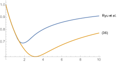
The proof is provided in Appendix 8. Observe that Proposition 3(1) is a new result, in which the Lipschitz constant of the explicit operator is improved with respect to considering a single operator when splitting is possible (see Remark 1). Proposition 3(2) provides a smaller Lipschitz-constant for operator $T_{\tau\mathcal{B},\tau\mathcal{A}}$ than in [38, Remarque 3.1(2)], [13, Theorem 2.4], [50, Proposition 1(d)], and [3, Proposition 26.16(ii)], by exploiting the cocoercivity of $\mathcal{A}$. On the other hand, in Proposition 3(3) we obtain a better Lipschitz constant for $T_{\tau\mathcal{A},\tau\mathcal{B}}$ than in [50, Proposition 1(d)] and [13, Theorem 2.4], and we recover the Lipschitz constant in [3, Proposition 26.16(i)], but we obtain a smaller Lipschitz constant by allowing $\tau=2\beta$. The Lipschitz constant of $R_{\tau\mathcal{A},\tau\mathcal{B}}$ and $R_{\tau\mathcal{B},\tau\mathcal{A}}$ in (35) is obtained in [28, Theorem 7.4], and it is smaller than Lipschitz constants in [28, Theorem 6.5 & Theorem 5.6] which are also valid in our context. The constant in (37) is provided in [28, Theorem 7.4] and it is tighter than the constant obtained in [35, Proposition 4], which does not take advantage of the full cocoercivity of the problem. The Lipschitz constant of $S_{\tau\mathcal{A},\tau\mathcal{B}}$ and $S_{\tau\mathcal{B},\tau\mathcal{A}}$ in (37) is obtained from [28, Theorem 5.6 & Theorem 7.4] by exploiting the cocoercivity of $\mathcal{A}$ and $\mathcal{B}$. When $\alpha$ is large with respect to $\beta$, our constant is sharper than the constant in [47, Corollary 4.2] (see Figure 1), which is obtained via computer-assisted analysis. This is because the cocoercivity of $\mathcal{A}$ is not considered in [47].

Rate vs step-size $\tau$

Figure 1: Comparison between the Lipschitz constants in [47] and (37) for DRS when $\beta=1$, $\rho=0.3$, and $\alpha=3$.

In the case when $\mathcal{B}=0$, by taking $\beta\to+\infty$ in parts 1 (or 2) and 3 of Proposition 3 we obtain as a direct consequence the following result for EA and PPA in the strongly monotone case. The Lipschitz continuous constant of EA obtained in [46, Fact 7] with a geometric proof is complemented with analytic arguments in the proof of Proposition 3. The constant of PPA is proved in [3, Proposition 23.13].

Proposition 4.

Suppose that $\mathcal{A}\in\mathcal{C}_{\alpha}$ is $\rho$-strongly monotone, for some $\alpha\in\left]0,+\infty\right[$ and $\rho\in\left]0,\alpha^{-1}\right]$. Then the following hold.

1. For every $\tau\in\left]0,2\alpha\right[$, $G_{\tau\mathcal{A}}$ is $\omega_{G_{0}}(\tau)$-Lipschitz continuous, where

   $$\omega_{G_{0}}:=\sqrt{1-\frac{\tau\rho}{\alpha}(2\alpha-\tau)}\in\left]0,1\right[.$$ (39)

2. For every $\tau>0$, $J_{\tau\mathcal{A}}$ is $\omega_{J}(\tau)$-Lipschitz continuous, where

   $$\omega_{J}(\tau):=\dfrac{1}{1+\tau\rho}\in\left]0,1\right[.$$ (40)

Remark 1.

Observe that $\mathcal{A}+\mathcal{B}$ is $\beta\alpha/(\beta+\alpha)$-cocoercive [3, Proposition 4.12] and $\rho$-strongly monotone. Moreover, for every $\tau\in\left]0,2\beta\alpha/(\beta+\alpha)\right[$ we have

$$\dfrac{\tau\rho}{\beta\alpha}\big{(}2\beta\alpha-\tau(\beta+\alpha)\big{)}<\frac{2\tau\rho}{\alpha(2\beta-\tau)}\big{(}2\beta\alpha-\tau(\beta+\alpha)\big{)}.$$ (41)

Therefore $\omega_{G}$ defined in (29) is strictly lower than $\omega_{G_{0}}$ in (39). Moreover, in the case when $\mathcal{B}=0$ ($\beta\to\infty$), both functions coincide. This new result implies that the gradient operator takes advantage of the splitting when a part of the monotone inclusion is strongly monotone.

Remark 2.

In the absence of strong monotonicity ($\rho=0$), EA, FBS, PRS, and DRS generate weakly convergent sequences. Indeed, even if the associated fixed point operators are no longer strict contractions, Proposition 8 in the appendix asserts that they are averaged nonexpansive operators, i.e., there exists $\mu\in\left]0,1\right[$ such that

$$(\forall x\in\mathcal{H})(\forall y\in\mathcal{H})\quad\|\Phi x-\Phi y\|^{2}\leq\|x-y\|^{2}-\left(\dfrac{1-\mu}{\mu}\right)\|(\operatorname{Id}-\Phi)x-(\operatorname{Id}-\Phi)y\|^{2}.$$ (42)

The weak convergence hence follows from [3, Proposition 5.16]. Note that, in the cocoercive context, the averaged nonexpansive property for the fixed point operator associated with PRS is a new result.

(a) Rate vs step-size $\tau$	(b) Rate vs step-size $\tau$

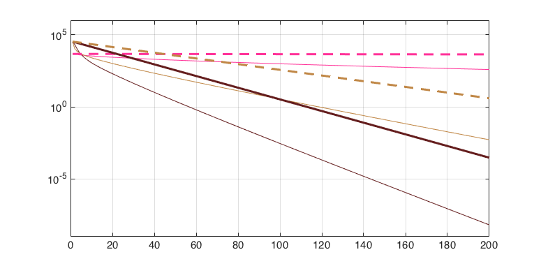
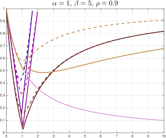
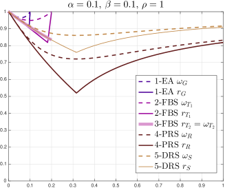
Figure 2: Comparison of the convergence rates of EA, FBS, PRS, DRS obtained in Proposition 5 (continuous lines) and Proposition 3 (dashed lines) for two choices of $\alpha$, $\beta$, and $\rho$. Note that optimization rates are better than cocoercive rates in general.

4 Smooth convex optimization

In this section we restrict our attention to the following particular instance of Problem 1.

Problem 2.

Let $(\alpha,\beta)\in\left]0,+\infty\right[^{2}$, let $\rho\in\left]0,\alpha^{-1}\right]$, let $f\in\mathscr{C}_{1/\alpha}^{1,1}(\mathcal{H})$ be $\rho$-strongly convex, and let $g\in\mathscr{C}_{1/\beta}^{1,1}(\mathcal{H})$. The problem is to

$$\underset{\begin{subarray}{c}{x\in\mathcal{H}}\end{subarray}}{\text{\rm minimize}}\;\;f(x)+g(x),$$ (43)

under the assumption that solutions exist.

In the context of Problem 2, there exists a unique solution to Problem 2, which is denoted by $\widehat{x}$. Since $\mathcal{A}=\nabla f$ is cocoercive and strongly monotone, Proposition 3 provides Lipschitz constants of the operators governing the numerical schemes under study. However, in the optimization setting the Lipschitz constants can be improved, as Proposition 5 below asserts. Next, we compare the convergence rates and we provide regions depending on the parameters $\alpha$, $\beta$, and $\rho$ defining the most efficient algorithm in the worst-case scenario.

4.1 Linear convergence rates

The following result is a refinement of Proposition 3, in which the Lipschitz constants are improved by using the convex optimization structure of the problem. All the linear convergence rates, optimal step-sizes, and associated optimal rates are summarized in Table 2.

Proposition 5.

Let $\tau>0$. In the context of Problem 2, the following hold:

1. Suppose that $\tau\in\left]0,2\beta\alpha/(\beta+\alpha)\right[$. Then, $G_{\tau(\nabla g+\nabla f)}$ is ${r}_{G}(\tau)$-Lipschitz continuous, where

   $${r}_{G}(\tau):=\max\big{\{}|1-\tau\rho|,|1-\tau(\beta^{-1}+\alpha^{-1})|\big{\}}\in\left]0,1\right[.$$ (44)

   In particular, the minimum in (44) is achieved at

   $$\tau^{*}=\dfrac{2}{\rho+\alpha^{-1}+\beta^{-1}}\quad\text{and}\quad{r}_{G}(\tau^{*})=\dfrac{\alpha^{-1}+\beta^{-1}-\rho}{\alpha^{-1}+\beta^{-1}+\rho}.$$ (45)

2. Suppose that $\tau\in\left]0,2\alpha\right[$. Then $T_{\tau\nabla g,\tau\nabla f}$ is $r_{T_{1}}(\tau)$-Lipschitz continuous, where

   $$r_{T_{1}}(\tau):=\max\big{\{}|1-\tau\rho|,|1-\tau\alpha^{-1}|\big{\}}\in\left]0,1\right[.$$ (46)

   In particular, the minimum in (46) is achieved at

   $$\tau^{*}=\dfrac{2}{\rho+\alpha^{-1}}\quad\text{ and }\quad{r}_{T_{1}}(\tau^{*})=\dfrac{\alpha^{-1}-\rho}{\alpha^{-1}+\rho}.$$ (47)

3. Suppose that $\tau\in\left]0,2\beta\right]$. Then $T_{\tau\nabla f,\tau\nabla g}$ is ${r}_{T_{2}}(\tau)$-Lipschitz continuous, where

   $${r}_{T_{2}}(\tau):=\dfrac{1}{1+\tau\rho}\in\left]0,1\right[.$$ (48)

   In particular, the minimum in (48) is achieved at

   $$\tau^{*}=2\beta\quad\text{ and }\quad{r}_{T_{2}}(\tau^{*})=\dfrac{1}{1+2\beta\rho}.$$ (49)

4. $R_{\tau\nabla g,\tau\nabla f}$ and $R_{\tau\nabla f,\tau\nabla g}$ are $r_{R}(\tau)$-Lipschitz continuous, where

   $$r_{R}(\tau)=\max\left\{\dfrac{1-\tau\rho}{1+\tau\rho},\dfrac{\tau\alpha^{-1}-1}{\tau\alpha^{-1}+1}\right\}\in\left]0,1\right[.$$ (50)

   In particular, the minimum in (50) is achieved at

   $$\tau^{*}=\sqrt{\frac{\alpha}{\rho}}\quad\text{ and }\quad{r}_{R}(\tau^{*})={\dfrac{1-\sqrt{\alpha\rho}}{1+\sqrt{\alpha\rho}}}.$$ (51)

5. $S_{\tau\nabla g,\tau\nabla f}$ and $S_{\tau\nabla f,\tau\nabla g}$ are $r_{S}(\tau)$-Lipschitz continuous, where

   $$r_{S}(\tau)=\min\left\{\frac{1+r_{R}(\tau)}{2},\dfrac{\beta+\tau^{2}\rho}{\beta+\tau\beta\rho+\tau^{2}\rho}\right\}\in\left]0,1\right[$$ (52)

   and $r_{R}$ is defined in (50). In particular, the optimal step-size and the minimum in (52) are

   $$(\tau^{*},r_{S}(\tau^{*}))=\begin{cases}\left(\sqrt{\frac{\alpha}{\rho}},\frac{1}{1+\sqrt{\alpha\rho}}\right),\quad&\text{if}\>\>\beta\leq{4\alpha};\\ \left(\sqrt{\frac{\beta}{\rho}},\frac{2}{2+\sqrt{\beta\rho}}\right),\quad&\text{otherwise}.\end{cases}$$ (53)

Algorithm	Linear convergence rate	Optimal step-size	Optimal linear
	as a function of $\tau$		convergence rate
EA with	$\max\big{\{}|1-\tau\rho|,|1-\tau(\beta^{-1}+\alpha^{-1})|\big{\}}$	$\dfrac{2}{\rho+\alpha^{-1}+\beta^{-1}}$	$\dfrac{\alpha^{-1}+\beta^{-1}-\rho}{\alpha^{-1}+\beta^{-1}+\rho}$
$\tau\in\left]0,2/(\alpha^{-1}+\beta^{-1})\right[$
FBS with ${\rm prox}_{g}$ and $\nabla f$	$\max\big{\{}|1-\tau\rho|,|1-\tau\alpha^{-1}|\big{\}}$	$\dfrac{2}{\rho+\alpha^{-1}}$	$\dfrac{\alpha^{-1}-\rho}{\alpha^{-1}+\rho}$
and $\tau\in\left]0,2\alpha\right[$
FBS with ${\rm prox}_{f}$ and $\nabla g$	$\dfrac{1}{1+\tau\rho}$	$2\beta$	$\dfrac{1}{1+2\beta\rho}$
and $\tau\in\left]0,2\beta\right]$
PRS with $\tau>0$	$\max\left\{\dfrac{1-\tau\rho}{1+\tau\rho},\dfrac{\tau\alpha^{-1}-1}{\tau\alpha^{-1}+1}\right\}$	$\dfrac{1}{1+2\beta\rho}$	${\dfrac{1-\sqrt{\alpha\rho}}{1+\sqrt{\alpha\rho}}}$
DRS with $\tau>0^{*}$	$\min\left\{\frac{1+r_{R}(\tau)}{2},\dfrac{\beta+\tau^{2}\rho}{\beta+\tau\beta\rho+\tau^{2}\rho}\right\}$	$\begin{cases}\sqrt{\frac{\alpha}{\rho}},\quad&\text{if}\>\>\beta\leq{4\alpha};\\ \sqrt{\frac{\beta}{\rho}},\quad&\text{otherwise}.\end{cases}$	$\begin{cases}\frac{1}{1+\sqrt{\alpha\rho}},\quad&\text{if}\>\>\beta\leq{4\alpha};\\ \frac{2}{2+\sqrt{\beta\rho}},\quad&\text{otherwise}.\end{cases}$

Table 2: Convergence rates and optimal step-sizes for several first-order schemes when considering the minimization problem $\min_{x\in\mathcal{H}}f(x)+g(x)$, where $f$ (resp. $g$) is convex differentiable with $\alpha^{-1}$ (resp. $\beta^{-1}$)-Lipschitz gradient and $f$ is $\rho$-strongly convex. ^∗ The results on DRS are new.

The Lipschitz constants of the operators $G_{\nabla g+\nabla f}$ and $T_{\nabla g,\nabla f}$ are a consequence of [49, Theorem 3.1] (see also [46, Fact 3] for a geometric interpretation). We provide an alternative shorter and more direct proof of Proposition 5(1)-(2) in Appendix 9, in which we use some techniques from [39, Section 2.1.3]. The Lipschitz constant of $T_{\nabla f,\nabla g}$ is a direct consequence of Proposition 3(3) and (50) is obtained in [29, Theorem 2], which improves several constants in the literature. The Lipschitz constant in (52) is obtained by combining [29, Theorem 2] and [28, Theorem 5.6].

Remark 3.

1. When $\rho\approx 0$, (47) justifies the classical choice $\tau^{*}\approx 2\alpha$. This case arises naturally in several inverse problems and, in particular, in sparse image restoration which is studied in detail in Section 5.2.

2. Note that the Lipschitz continuous constants obtained in Proposition 5(1) and 5(2) are strictly lower than the constants obtained in Proposition 3(1) and 3(2) in the cocoercive case, as it can be verified in Figure 2.

3. From Figure 2, we observe the benefit of the refinement of convergence rates in the optimization framework (dashed line) with respect to the cocoercive case (solid line) in all methods at exception of $T_{\tau\nabla f,\tau\nabla g}$, whose rate is the same. We also observe that in general Peaceman-Rachford iterations $R_{\tau\nabla g,\tau\nabla f}$ has the better convergence rate for several configurations of $(\alpha,\beta,\rho)$.
   

In the case when $g=0\in\mathscr{C}_{0}^{1,1}(\mathcal{H})$, Problem 2 reduces to minimize $f$ over $\mathcal{H}$ and $G_{\nabla g+\nabla f}=T_{\nabla g,\nabla f}=G_{\nabla f}$ and $T_{\nabla f,\nabla g}=S_{\nabla f,\nabla g}=S_{\nabla g,\nabla f}={\rm prox}_{f}$. Therefore, by taking $\beta\to+\infty$ in Proposition 5, we recover the following known results (see also [28, Proposition 5.2] and [3, Proposition 4.39]).

Proposition 6.

Let $\tau\in\left]0,+\infty\right[$, $\alpha\in\left]0,+\infty\right[$, $\rho\in\left]0,\alpha^{-1}\right]$, and suppose that $f\in\mathscr{C}^{1,1}_{1/\alpha}(\mathcal{H})$ and that $f$ is $\rho$-strongly convex. Then, the following hold.

1. Suppose that $\tau\in\left]0,2\alpha\right[$. Then $G_{\tau\nabla f}$ is $r_{G_{0}}(\tau)$-Lipschitz continuous, where

   $$r_{G_{0}}(\tau):=\max\big{\{}|1-\tau\rho|,|1-\tau\alpha^{-1}|\big{\}}\in\left]0,1\right[.$$ (54)

2. ${\rm prox}_{\tau f}$ is ${r}_{J}(\tau)$-Lipschitz continuous, where

   $${r}_{J}(\tau):=\dfrac{1}{1+\tau\rho}\in\left]0,1\right[.$$ (55)

4.2 Comparison of algorithms

Since Problem 2 is equivalent to minimize $\alpha f+\alpha g$ over $\mathcal{H}$, we can assume $\alpha=1$. Set $\Omega=\left]0,+\infty\right[\times\left]0,1\right[$ and denote

$$\begin{cases}r_{G}^{*}(\beta,\rho)=\frac{1+\beta^{-1}-\rho}{1+\beta^{-1}-\rho}\\ r_{T_{1}}^{*}(\rho)=\frac{1-\rho}{1+\rho}\\ r_{T_{2}}^{*}(\beta,\rho)=\frac{1}{1+2\beta\rho}\\ r_{R}^{*}(\rho)=\frac{1-\sqrt{\rho}}{1+\sqrt{\rho}}\\ r_{S}^{*}(\beta,\rho)=\begin{cases}\frac{1}{1+\sqrt{\rho}},&\text{if}\>\>\beta\leq 4;\\ \frac{2}{2+\sqrt{\beta\rho}},&\text{if}\>\>\beta>4.\end{cases}\end{cases}$$ (56)

Observe that $r_{G}^{*}(\beta,\rho)=r_{G}(\tau^{*})$, $r_{T_{1}}^{*}(\rho)=r_{T_{1}}(\tau^{*})$, $r_{T_{2}}^{*}(\beta,\rho)=r_{T_{2}}(\tau^{*})$, $r_{R}^{*}(\rho)=r_{R}(\tau^{*})$, and $r_{S}^{*}(\beta,\rho)=r_{S}(\tau^{*})$ are the optimal rates obtained in Proposition 5 when $\alpha=1$. We have the following comparisons.

Lemma 1.

Let $(\beta,\rho)\in\Omega$. Then $r_{G}^{*}(\beta,\rho)>r_{T_{1}}^{*}(\rho)>r_{R}^{*}(\rho)$.

Proof.

Set

$$\phi\colon(t,\rho)\mapsto\frac{t-\rho}{t+\rho}=1-\frac{2}{1+t/\rho}$$ (57)

and note that, for every $(t,\rho)\in\left]0,+\infty\right[\times\left]0,1\right[$, $\phi(\cdot,\rho)$ is strictly increasing on $\left]0,+\infty\right[$ and $\phi(t,\cdot)$ is strictly decreasing on $\left]0,1\right[$. Noting that $\sqrt{\rho}>\rho$, the result follows from $r_{G}^{*}(\beta,\rho)=\phi(1+\beta^{-1},\rho)>\phi(1,\rho)=r_{T_{1}}^{*}(\rho)$ and $r_{T_{1}}^{*}(\rho)=\phi(1,\rho)>\phi(1,\sqrt{\rho})=r_{R}^{*}(\rho)$. ∎

We conclude from Lemma 1 that PRS is always more efficient than the algorithms governed by operators $T_{\tau^{*}\nabla g,\tau^{*}\nabla f}$ and $G_{\tau^{*}(\nabla g+\nabla f)}$ for solving Problem 2. Therefore, it is enough to compare $r_{R}^{*}(\rho)$, $r_{T_{2}}^{*}(\beta,\rho)$, and $r_{S}^{*}(\beta,\rho)$.

Lemma 2.

Let $(\beta,\rho)\in\Omega$. The following hold:

1. $r_{T_{2}}^{*}(\beta,\rho)<r_{R}^{*}(\rho)\>\Leftrightarrow\>\beta>4\>\>\text{and}\>\>\beta\rho\in\left]\eta(\beta),\eta(\beta)^{-1}\right[$, where

   $$\eta(\beta)=\frac{1-\sqrt{1-4\beta^{-1}}}{1+\sqrt{1-4\beta^{-1}}}\in\left]0,1\right[.$$ (58)

2. $r_{S}^{*}(\beta,\rho)<r_{R}^{*}(\rho)\>\>\Leftrightarrow\>\>\beta>16\>\>\>\text{and}\>\>\>\rho<1-8(\frac{\sqrt{\beta}-2}{\beta}).$

3. Suppose that $\beta>4$. Then $r_{S}^{*}(\beta,\rho)<r_{T_{2}}^{*}(\beta,\rho)\>\>\Leftrightarrow\>\>\rho<\frac{1}{16\beta}.$

Proof.

1: Note that

$$r_{T_{2}}^{*}(\beta,\rho)-r_{R}^{*}(\rho)=\frac{1}{1+2\beta\rho}-\frac{1-\sqrt{\rho}}{1+\sqrt{\rho}}=\frac{1+\sqrt{\rho}-(1-\sqrt{\rho})(1+2\beta\rho)}{(1+2\beta\rho)(1+\sqrt{\rho})}=\frac{2\sqrt{\rho}\beta(\rho-\sqrt{\rho}+\beta^{-1})}{(1+2\beta\rho)(1+\sqrt{\rho})}.$$ (59)

Hence, $r_{T_{2}}^{*}(\beta,\rho)<r_{R}^{*}(\rho)$ is equivalent to $1-4\beta^{-1}>0$ and $\sqrt{\rho}\in\left]\eta_{1},\eta_{2}\right[$, where $\eta_{1}=(1-\sqrt{1-4\beta^{-1}})/2$ and $\eta_{2}=(1+\sqrt{1-4\beta^{-1}})/2$, which yields the result after simple computations.

2: It is clear from (56) that, when $\beta\leq 4$, $r_{S}^{*}(\beta,\rho)\geq r_{R}^{*}(\rho)$. Hence, by assuming that $\beta>4$, we have

$$r_{S}^{*}(\beta,\rho)-r_{R}^{*}(\rho) =\frac{2}{2+\sqrt{\beta\rho}}-\frac{1-\sqrt{\rho}}{1+\sqrt{\rho}}=\frac{4\sqrt{\rho}-\sqrt{\beta\rho}(1-\sqrt{\rho})}{(2+\sqrt{\beta\rho})(1+\sqrt{\rho})}=\frac{\sqrt{\rho}(4-\sqrt{\beta}+\sqrt{\beta\rho})}{(2+\sqrt{\beta\rho})(1+\sqrt{\rho})}.$$ (60)

We observe that, for every $\beta\leq 16$, we have $r_{S}^{*}(\beta,\rho)\geq r_{R}^{*}(\rho)$ and, if $\beta>16$, $r_{S}^{*}(\beta,\rho)<r_{R}^{*}(\rho)$ if and only if $\sqrt{\rho}<1-4/\sqrt{\beta}$, from which the result follows.

3: Since

$$r_{S}^{*}(\beta,\rho)-r_{T_{2}}^{*}(\beta,\rho)=\frac{2}{2+\sqrt{\beta\rho}}-\frac{1}{1+2\beta\rho}=\frac{\sqrt{\beta\rho}(4\sqrt{\beta\rho}-1)}{(2+\sqrt{\beta\rho})(1+2\beta\rho)},$$ (61)

the proof is complete. ∎

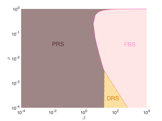
Now, by using Lemma 2, we can conclude which algorithm has the lower convergence rate depending on the parameters $(\beta,\rho)\in\Omega$. In Figure 3 we illustrate the efficiency regions thus derived and Table 3 summarizes the result of Lemma 2.

Proposition 7.

Let $(\beta,\rho)\in\Omega$ and let $\eta$ be the function defined in (58). Then, the following hold:

1. Suppose that $\beta>4$ and that $\rho\in I(\beta)$, where

   $$I(\beta)=\left[\frac{\max\{1/16,\eta(\beta)\}}{\beta},\frac{1}{\beta\eta(\beta)}\right].$$

   Then $r_{T_{2}}^{*}(\beta,\rho)\leq\min\{r_{S}^{*}(\beta,\rho),r_{R}^{*}(\rho)\}$.

2. Suppose that $\beta>16$ and that $\rho<\chi(\beta)$, where

   $$\chi(\beta)=\min\left\{\frac{1}{16\beta},1-8\frac{\sqrt{\beta}-2}{\beta}\right\}.$$

   Then $r_{S}^{*}(\beta,\rho)<\min\{r_{T_{2}}^{*}(\beta,\rho),r_{R}^{*}(\rho)\}$.

In any other case, we have $r_{R}^{*}(\rho)\leq\min\{r_{T_{2}}^{*}(\beta,\rho),r_{S}^{*}(\beta,\rho)\}$.

5 Numerical experiments

The theoretical results provided in the previous sections are now illustrated on standard data processing examples with different levels of complexity: Piecewise-constant denoising and image restoration. The Matlab codes associated with the following experiments are available on Nelly Pustelnik website (link).

5.1 Piecewise constant denoising

Piecewise constant denoising (also referred as change-point detection) is a very well documented problem of signal processing literature and it is of interest for numerous signal processing applications going from genomics [52] to geophysics studies [41].

Region of parameters $(\beta,\rho)$	Algorithm with the best rate
$\Omega_{1}=\Big{\{}(\beta,\rho)\,|\,\beta>4\;\;\mbox{and}\;\;\rho\in\big{[}\frac{\max\{1/16,\eta(\beta)\}}{\beta},\frac{1}{\beta\eta(\beta)}\Big{]}\Big{\}}$	FBS with ${\rm prox}_{\tau f}$
$\Omega_{2}=\Big{\{}(\beta,\rho)\,|\,\beta>4\;\;\mbox{and}\;\;\rho\in\Big{[}\frac{1}{16\beta},1-8\frac{\sqrt{\beta}-2}{\beta}\Big{]}\Big{\}}$	DRS
$\Omega\setminus(\Omega_{1}\cup\Omega_{2})$	PRS

Table 3: Best rate algorithms among EA, FBS with prox or gradient activation of the strongly convex function, DRS, PRS when $\alpha=1$ when considering the minimization problem $\min_{x\in\mathcal{H}}f(x)+g(x)$, where $f$ (resp. $g$) is convex differentiable with $\alpha^{-1}$ (resp. $\beta^{-1}$)-Lipschitz gradient and $f$ is $\rho$-strongly convex.

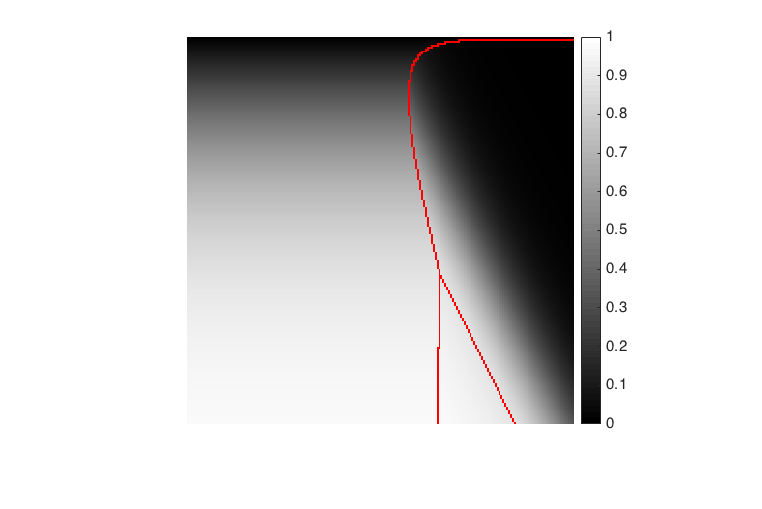
Figure 3: (Left) Regimes where PRS or FBS or DRS achieves a better rate according to Proposition 7 when $\alpha=1$ as a function of $(\beta,\rho)$. (Right) Optimal numerical rates and associated regions.

The standard formulation is dedicated to piecewise constant signal $\overline{x}\in\mathbb{R}^{N}$ degraded with a Gaussian noise $\varepsilon\sim\mathcal{N}(0,\sigma^{2}\mathbb{I})$, whose degraded version is denoted $z=\overline{x}+\varepsilon$. An illustration of $\overline{x}$ (resp. $z$) is provided in solid black line (resp. gray) in Figure 4 (top).

The estimation of a piecewise constant signal $\widehat{x}$ from degraded data $z$ has been addressed by several strategies going from Cusum procedures [2], hierarchical Bayesian inference frameworks [31], or functional optimization formulations involving $\ell_{1}$-norm or the $\ell_{0}$-pseudo-norm of the first differences of the signal (see e.g. [27] and references therein). In the latter context, we consider the minimization problem:

$$\underset{\begin{subarray}{c}{x\in\mathbb{R}^{N}}\end{subarray}}{\text{\rm minimize}}\;\;\frac{1}{2}\|x-z\|_{2}^{2}+\chi h_{\mu}(Dx),$$ (62)

where $D\in\mathbb{R}^{N-1\times N}$ denotes the first-order discrete difference operator

$$(\forall n\in\{1,\ldots,N-1\})\quad(Dx)_{n}=\frac{1}{2}(x_{n}-x_{n-1})$$

and $h_{\mu}\colon\mathbb{R}^{N-1}\to\mathbb{R}$ denotes the Huber loss of parameter $\mu>0$, which is a smooth approximation of the $\ell_{1}$-norm defined by (see, e.g., [15, Example 2.5])

$$h_{\mu}\colon(\zeta_{i})_{1\leq i\leq m}\mapsto\sum_{i=1}^{N-1}\phi_{\mu}(\zeta_{i})\quad\text{and}\quad\phi_{\mu}\colon\zeta\mapsto\left\{\begin{array}[]{ll}{|\zeta|-\frac{\mu}{2},}&{\text{ if }|\zeta|>\mu};\\ {\frac{|\zeta|^{2}}{2\mu},}&{\text{ if }|\zeta|\leqslant\mu}.\end{array}\right.$$ (63)

Note that, since

$$\phi^{\prime}_{\mu}\colon\zeta\mapsto\left\{\begin{array}[]{ll}{\frac{\zeta}{|\zeta|},}&{\text{ if }|\zeta|>\mu};\\ {\frac{\zeta}{\mu},}&{\text{ if }|\zeta|\leqslant\mu},\end{array}\right.$$

we have $h_{\mu}\in\mathscr{C}^{1,1}_{1/\mu}(\mathbb{R}^{N-1})$. By setting $f=\frac{1}{2}\|\cdot-z\|_{2}^{2}$ and $g=\chi h_{\mu}\circ D$, (62) is a particular instance of Problem 2, where $f$ is $\rho=1$ strongly convex, $\alpha=1$, and $\beta=\frac{\mu}{{\chi}\|D\|^{2}}$ and it can be solved by the following two schemes:

1. EA: Use $G_{\tau(\nabla g+\nabla f)}$ with the step-size $\tau^{*}$ in (45).

2. FBS: Use $T_{\tau\nabla f,\tau\nabla g}$ with the step-size $\tau^{*}$ in (49).

Moreover, the proximity operator of $h_{\mu}$ can be computed explicitly via

$$(\forall\tau>0)\quad{\rm prox}_{\tau h_{\mu}}\colon(\zeta_{i})_{1\leq i\leq m}\mapsto({\rm prox}_{\tau\phi_{\mu}}\zeta_{i})_{1\leq i\leq m},$$ (64)

where

$${\rm prox}_{\tau\phi_{\mu}}\colon\zeta\mapsto\left\{\begin{array}[]{ll}{\zeta-\frac{\tau\zeta}{|\zeta|},}&{\text{ if }|\zeta|>\tau+\mu};\\ {\frac{\mu\zeta}{\tau+\mu},}&{\text{ if }|\zeta|\leqslant\tau+\mu}.\end{array}\right.$$ (65)

However, the proximity operator of $h_{\mu}\circ D$ is not explicit because of the influence of operator $D$. By exploiting the separable structure of $h_{\mu}$, we obtain the following equivalent formulation of (62):

$$\min_{x\in\mathcal{H}}\frac{1}{2}\|x-z\|_{2}^{2}+\chi h_{\mathbb{I}_{1}}(D_{\mathbb{I}_{1}}x)+\chi h_{\mathbb{I}_{2}}(D_{\mathbb{I}_{2}}x),$$ (66)

where $\mathbb{I}_{1}=\{1,3,\ldots\}$ and $\mathbb{I}_{2}=\{2,4,\ldots\}$ are the sets of odd and even indices and, for $k\in\{1,2\}$, $h_{\mathbb{I}_{k}}(y_{\mathbb{I}_{k}})=\sum_{i\in\mathbb{I}_{k}}\phi_{\mu}(y_{i})$, and $D_{\mathbb{I}_{k}}\in\mathbb{R}^{|\mathbb{I}_{k}|\times N}$ denotes the sub-matrix of $D$ associated with the $\mathbb{I}_{k}$ rows. Since $D_{\mathbb{I}_{1}}D_{\mathbb{I}_{1}}^{\top}=\textrm{Id}/2$ and $D_{\mathbb{I}_{2}}D_{\mathbb{I}_{2}}^{\top}=\textrm{Id}/2$, the split formulation (66) allows for the following closed form expressions of the proximity operator of $h_{\mathbb{I}_{k}}\circ D_{\mathbb{I}_{k}}$ (see [3, Proposition 23.25])

$$(\forall k\in\{1,2\})(\forall\tau>0)\quad{\rm prox}_{\tau h_{\mathbb{I}_{k}}\circ D_{\mathbb{I}_{k}}}\colon z\mapsto z-2L_{\mathbb{I}_{k}}^{\top}\big{(}\operatorname{Id}-{\rm prox}_{\frac{\tau}{2}h_{\mathbb{I}_{k}}}\big{)}(D_{\mathbb{I}_{k}}z),$$

where ${\rm prox}_{\frac{\tau}{2}h_{\mathbb{I}_{k}}}\colon(\zeta_{i})_{i\in\mathbb{I}_{k}}\mapsto({\rm prox}_{\frac{\tau}{2}\phi_{\mu}}\zeta_{i})_{i\in\mathbb{I}_{k}}$. By setting $\widetilde{f}=\frac{1}{2}\|\cdot-z\|_{2}^{2}+\chi h_{\mathbb{I}_{2}}(D_{\mathbb{I}_{2}}\cdot)$ and $\widetilde{g}=\chi h_{\mathbb{I}_{1}}(D_{\mathbb{I}_{1}}\cdot)$, we write (66) as Problem 2, where $\widetilde{f}$ is $\rho=1$ strongly convex, $\alpha=\frac{\mu}{\mu+{\chi}\|D_{\mathbb{I}_{2}}\|^{2}}$, and $\beta=\frac{\mu}{{\chi}\|D_{\mathbb{I}_{1}}\|^{2}}$. This approach gives raise to 4 alternative methods for solving (66).

1. FBS 2: Use $T_{\tau\nabla\widetilde{g},\tau\nabla\widetilde{f}}$ with the step-size $\tau^{*}$ in (47).

2. FBS 3: Use $T_{\tau\nabla\widetilde{f},\tau\nabla\widetilde{g}}$ with the step-size $\tau^{*}$ in (49).

3. PRS: Use $R_{\tau\nabla\widetilde{f},\tau\nabla\widetilde{g}}$ with the step-size $\tau^{*}$ in (51).

4. DRS: Use $S_{\tau\nabla\widetilde{f},\tau\nabla\widetilde{g}}$ with the step-size $\tau^{*}$ in (53).

We consider an approximation of the unique solution $\widehat{x}$ to (62), by applying PRS with a large number of iterations. In view of Section 2.4, 1-EA, 2-FBS, 3-FBS2, and 4-FBS3 are initialized with $x_{0}=z$, while using

$$z={\rm prox}_{\gamma f}(x_{n})\Leftrightarrow(\operatorname{Id}+\gamma\nabla f)y_{n}=x_{n}$$

proximal-based procedures 5-PRS and 6-DRS are initialized by $x_{0}=z+\tau\nabla f(z)$, in order to provide similar initializations.

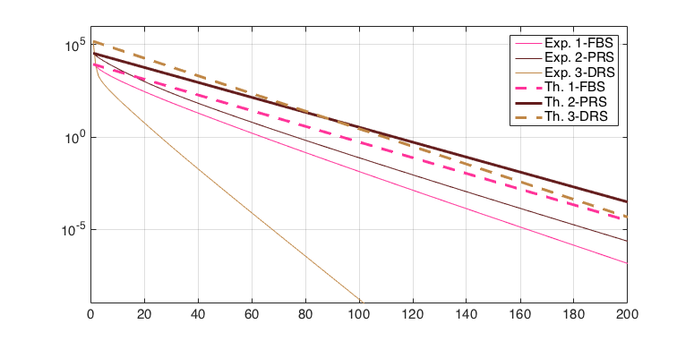
The numerical and theoretical convergence rate are displayed in Figure 4 for different settings of $\mu$ and $\chi$ leading to sharper or smoother estimates depending of the configuration. When $\mu=10^{-4}$ the performance are similar to what is expected for $\ell_{1}$-minimization.

From Figure 4 (bottom), we can observe that PRS iterations provide the best theoretical and experimental rates when the optimal step-size is selected. DRS iterations also provide a good behavior, while EA and FBS strategies relying on the splitting $f=\frac{1}{2}\|\cdot-z\|_{2}^{2}$ and $g=\chi h_{\mu}\circ D$ appears less efficient than the one involving the splitting $\widetilde{f}=\frac{1}{2}\|\cdot-z\|_{2}^{2}+\chi h_{\mathbb{I}_{2}}(D_{\mathbb{I}_{2}}\cdot)$ and $\widetilde{g}=\chi h_{\mathbb{I}_{1}}\circ D_{\mathbb{I}_{1}}$. Similar conclusion can be observed from Figure 4 (top), where the optimal solution is reached after 100 iterations for DRS (light brown) and PRS (dark brown) while gradient based procedures require much more iterations. This is especially true when $\mu$ is small, leading to a large Lipschitz constant and, thus, to a small step-size for gradient-based algorithms. Moreover, observe that our results are consistent with Proposition 7 illustrated in Figure 3. Since $\alpha=\rho=1$, we verify that PRS is the most efficient algorithm and that EA and FBS are not competitive.

(a) Original/degraded/reconstructed signals	(b) Original/degraded/reconstructed signals
(c) Errors vs Iterations	(d) Errors vs Iterations

Figure 4: Piecewise constant denoising estimates after 10, 100, and 10000 iterations with $\chi=0.7$ and $\mu=0.0001$ (a) and $\chi=0.7$ and $\mu=0.002$ (b). We can observe that the piecewise constant estimate is obtained after 100 iterations for DRS or PRS while EA or FBS requires much more iterations. We also exhibit the experimental and theoretical errors associated with each implemented method for optimal step-size $\tau$ with respect to iteration number (c-d). The behavior is in accordance with the results observed on the first row.

5.2 Image restoration

Another classical signal processing problem is image restoration that consists in recovering an image $\overline{x}\in\mathbb{R}^{N}$ with $N$ pixels from degraded observations $z=A\overline{x}+\varepsilon$, where $A\in\mathbb{R}^{M\times N}$ with $M\geq N$ and $\varepsilon\sim\mathcal{N}(0,\sigma^{2}\mathbb{I})$ is a white Gaussian noise. A standard penalization imposes the sparsity of the coefficients resulting from a linear transform such as a wavelet transform [44] and the restoration can then be achieved by solving

$$\underset{{x\in\mathcal{H}}}{\textrm{minimize}}\;\frac{1}{2}\|Ax-z\|_{2}^{2}+\chi h_{\mu}(Wx),$$ (67)

where $\chi>0$ is the regularization parameter, $W$ denotes a weighted wavelet transform, and $h_{\mu}$ is the Huber penalization of parameter $\mu>0$ defined in (63).

Following Proposition 7, we propose to evaluate the theoretical and the experimental rates for the following algorithmic schemes, where $f=\frac{1}{2}\|A\cdot-z\|_{2}^{2}$ and $g=\chi h_{\mu}\circ W$:

1. FBS: Use $T_{\tau\nabla f,\tau\nabla g}$ with the step-size $\tau^{*}$ in (49).

2. PRS: Use $R_{\tau\nabla f,\tau\nabla g}$ with the step-size $\tau^{*}$ in (51).

3. DRS: Use $S_{\tau\nabla f,\tau\nabla g}$ with the step-size $\tau^{*}$ in (53).

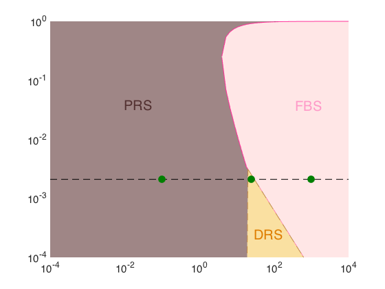
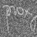
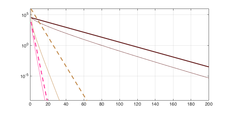
In this context, by denoting $\lambda_{\max}$ and $\lambda_{\min}$ the largest and lowest eigenvalues of $A^{\top}A$, $\rho=\lambda_{\min}$ is the strong convexity parameter of $f$, $\lambda_{\max}=\alpha^{-1}$ is the Lipschitz constant of $\nabla f$, and $\beta^{-1}=\frac{\chi}{\mu}$ is the Lipschitz constant of $\nabla g$. The results are displayed in Figure 5 for an image with $N=2^{12}$ pixels when $A$ is a random Gaussian matrix of size $4900\times 4096$ with $\lambda_{\min}=0.0022$ and $\lambda_{\max}=1$. The results are obtained considering three values of $\chi\in\{0.001,0.04,10\}$ and $\mu=1$ in order to consider three instances (green dots) in the three different efficiency regions (displayed in brown, orange, and pink).

Original
$A^{-1}z$
Image restored with PRS with $\beta=0.1$ and convergence behavior for the different schemes.
Image restored with DRS with $\beta=25$ and convergence behavior for the different schemes.
Image restored with FBS with $\beta=1000$ and convergence behavior for the different schemes.

Figure 5: Image restoration example considering a random matrix. The figure at the top right includes in Figure 3 a dashed black line and three green dots representing the cases explored in this experiment ($\rho=\lambda_{\min}=0.0022$, $\alpha=1/\lambda_{\max}=1$, $\mu=1$, and $\beta=\mu/\chi\in\{0.1,25,1000\}$). We verify that the theoretical and numerical errors decay as predicted in Proposition 7.

The first set of experiments (second row in Figure 5) displays the results obtained with $\chi=10$ ($\beta=0.1$). In this case, PRS achieves a better rate according to the theoretical study in Proposition 7 (brown region in Figure 3) and our numerical experiments confirm this result. The third (fourth) row displays the results obtained with $\chi=0.04$ (resp. $\chi=0.001$) and, thus, $\beta=25$ (resp. $\beta=1000$), associated with the orange (resp. pink) efficiency region where DRS (resp. FBS) leads to the best theoretical rate. In this context where the strong convexity constant is small, the fit between theoretical and numerical convergence behaviour is not as tight. The best restoration results are obtained when $\chi=10$, in which case PRS performs better.

6 Cocoercivity and strong monotonicity in Example 1

Consider the operators $\mathcal{A}$ and $\mathcal{B}$ defined in (27), and fix $(x_{1},u_{1})$ and $(x_{2},u_{2})$ in $\mathbb{R}^{n}\times\mathbb{R}^{p}$. For every $(y_{1},v_{1})\in\mathcal{A}(x_{1},u_{1})$ and $(y_{2},v_{2})\in\mathcal{A}(x_{2},u_{2})$, since $h^{*}$ is $1/L$-strongly convex [3, Theorem 18.15], we have

$${\left\langle{{(y_{1},v_{1})-(y_{2},v_{2})}\mid{(x_{1},u_{1})-(x_{2},u_{2})}}\right\rangle} ={\left\langle{{\nabla f(x_{1})-\nabla f(x_{2})}\mid{x_{1}-x_{2}}}\right\rangle}-\eta\|x_{1}-x_{2}\|^{2}$$

$$\qquad+{\left\langle{{v_{1}+\eta u_{1}-(v_{2}+\eta u_{2})}\mid{u_{1}-u_{2}}}\right\rangle}-\eta\|u_{1}-u_{2}\|^{2}$$

$$\geq(\mu-\eta)\|x_{1}-x_{2}\|^{2}+(1/L-\eta)\|u_{1}-u_{2}\|^{2}$$

$$\geq(\min\{\mu,1/L\}-\eta)\|(x_{1},u_{1})-(x_{2}-u_{2})\|^{2},$$ (68)

which implies the $(\min\{\mu,1/L\}-\eta)$-strong convexity of $\mathcal{A}$. Moreover, in the case when $h$ is also $\rho$-strongly convex, we have $h^{*}\in\mathscr{C}_{1/\rho}^{1,1}(\mathbb{R}^{p})$, $\mathcal{A}\colon(x,u)\mapsto(\nabla f({x})-\eta x,\nabla h^{*}({u})-\eta u)$ is single valued and

$${\left\langle{{\mathcal{A}(x_{1},u_{1})-\mathcal{A}(x_{2},u_{2})}\mid{(x_{1},u_{1})-(x_{2},u_{2})}}\right\rangle} ={\left\langle{{\nabla f(x_{1})-\nabla f(x_{2})}\mid{x_{1}-x_{2}}}\right\rangle}-\eta\|x_{1}-x_{2}\|^{2}$$

$$\qquad+{\left\langle{{\nabla h^{*}(u_{1})-\nabla h^{*}(u_{2})}\mid{u_{1}-u_{2}}}\right\rangle}-\eta\|u_{1}-u_{2}\|^{2}$$

$$\geq\frac{1}{\|A\|^{2}}\|\nabla f(x_{1})-\nabla f(x_{2})\|^{2}+\rho\|\nabla h^{*}(u_{1})-\nabla h^{*}(u_{2})\|^{2}.$$ (69)

On the other hand, the strong monotonicity of $\nabla f$ and $\nabla h^{*}$ imply $\|\nabla f(x_{1})-\nabla f(x_{2})\|\geq\mu\|x_{1}-x_{2}\|$ and $\|\nabla h^{*}(u_{1})-\nabla h^{*}(u_{2})\|\geq(1/L)\|u_{1}-u_{2}\|$, which yield

$$\|\mathcal{A}(x_{1},u_{1})-\mathcal{A}(x_{2},u_{2})\| \leq\|\nabla f(x_{1})-\nabla f(x_{2})\|+\eta\|x_{1}-x_{2}\|+\|\nabla h^{*}(u_{1})-\nabla h^{*}(u_{2})\|+\eta\|u_{1}-u_{2}\|$$

$$\leq(1+\eta/\mu)\|\nabla f(x_{1})-\nabla f(x_{2})\|+(1+\eta L)\|\nabla h^{*}(u_{1})-\nabla h^{*}(u_{2})\|.$$ (70)

Therefore, it follows from (6) that $\mathcal{A}$ is $(\min\{\rho,\|A\|^{-2}\}/(1+\eta\max\{(1/\mu,L\})^{2})$-cocoercive. Finally,

$${\left\langle{{\mathcal{B}(x_{1},u_{1})-\mathcal{B}(x_{2},u_{2})}\mid{(x_{1},u_{1})-(x_{2},u_{2})}}\right\rangle} =\eta\|x_{1}-x_{2}\|^{2}+{\left\langle{{D^{\top}(x_{1}-x_{2})}\mid{x_{1}-x_{2}}}\right\rangle}$$

$$\qquad+\eta\|u_{1}-u_{2}\|^{2}-{\left\langle{{D(x_{1}-x_{2})}\mid{u_{1}-u_{2}}}\right\rangle}$$

$$=\eta\|(x_{1},u_{1})-(x_{2}-u_{2})\|^{2}$$

$$\geq\frac{\eta}{\|\mathcal{B}\|^{2}}\|\mathcal{B}(x_{1},u_{1})-\mathcal{B}(x_{2}-u_{2})\|^{2},$$ (71)

which implies the $\eta/\|\mathcal{B}\|^{2}$-cocoercivity of $\mathcal{B}$.

7 Averaged nonexpansive constants in the case $\rho=0$

Proposition 8.

Let $\tau>0$. In the context of Problem 1, the following hold:

1. Suppose that $\tau\in\left]0,2\beta\alpha/(\beta+\alpha)\right[$. Then $G_{\tau(\mathcal{A}+\mathcal{B})}$ is $\mu_{G}(\tau)$-averaged nonexpansive, where

   $$\mu_{G}(\tau):=\frac{\tau(\beta+\alpha)}{2\beta\alpha}\in\left]0,1\right[.$$ (72)

2. Suppose that $\tau\in\left]0,2\alpha\right[$. Then $T_{\tau\mathcal{B},\tau\mathcal{A}}$ is $\mu_{T}(\tau)$-averaged nonexpansive, where

   $$\mu_{T}(\tau):=\frac{2\tau(\beta+\alpha)}{4\beta\alpha+\tau(4\alpha-\tau)}\in\left]0,1\right[.$$ (73)

3. $R_{\tau\mathcal{B},\tau\mathcal{A}}$ is $\mu_{R}(\tau)$-averaged nonexpansive, where

   $$\mu_{R}(\tau):=\dfrac{\tau}{\frac{\alpha\beta}{\alpha+\beta}+\tau}\in\left]0,1\right[.$$ (74)

4. $S_{\tau\mathcal{B},\tau\mathcal{A}}$ is $\mu_{S}(\tau)=\frac{\mu_{R}(\tau)}{2}$-averaged nonexpansive.

Proof.

1: It follows from [3, Proposition 4.12] that $\mathcal{A}+\mathcal{B}$ is $(\beta^{-1}+\alpha^{-1})^{-1}=\alpha\beta/(\alpha+\beta)$-cocoercive.

The result thus follows from [3, Proposition 4.39].

2: Since $\tau\mathcal{B}$ is $\beta/\tau$-cocoercive, it follows from [28, Proposition 5.2] and [3, Proposition 4.39] that $J_{\tau\mathcal{B}}$ and $G_{\tau\mathcal{A}}$ are $\alpha_{\mathcal{B}}=\tau/(2(\tau+\beta))\in\left]0,1/2\right[$ and $\alpha_{\mathcal{A}}=\tau/(2\alpha)$-averaged nonexpansive, respectively. Hence, we deduce from [19, Proposition 2.4] that $T_{\tau\mathcal{B},\tau\mathcal{A}}=J_{\tau\mathcal{B}}\circ G_{\tau\mathcal{A}}$ is averaged with constant $(\alpha_{\mathcal{B}}+\alpha_{\mathcal{A}}-2\alpha_{\mathcal{B}}\alpha_{\mathcal{A}})/(1-\alpha_{\mathcal{B}}\alpha_{\mathcal{A}})$ which leads the result after simple computations.

3: Since $\tau\mathcal{A}$ and $\tau\mathcal{B}$ are $\alpha/\tau$- and $\beta/\tau$-cocoercive, respectively, it follows from [28, Proposition 5.3] that $R_{\tau\mathcal{A}}=2J_{\tau\mathcal{A}}-\operatorname{Id}$ and $R_{\tau\mathcal{B}}=2J_{\tau\mathcal{B}}-\operatorname{Id}$ are $\tau/(\tau+\alpha)$ and $\tau/(\tau+\beta)$ averaged nonexpansive, respectively. Hence, since $R_{\tau\mathcal{B},\tau\mathcal{A}}=R_{\tau\mathcal{B}}\circ R_{\tau\mathcal{A}}$, the averaging constant is obtained from [19, Proposition 2.4] as in 2.

4: Since $S_{\tau,\mathcal{B},\mathcal{A}}=(\operatorname{Id}+R_{\tau\mathcal{B}}\circ R_{\tau\mathcal{A}})/2$ we deduce the result from 3 and [3, Proposition 4.40]. ∎

8 Proof of Proposition 3

1: Set $\mathcal{M}=\mathcal{A}+\mathcal{B}$, fix $\tau\in\left]0,2\beta\alpha/(\beta+\alpha)\right[\subset\left]0,2\min\{\beta,\alpha\}\right[$, fix $x$ and $y$ in $\mathcal{H}$. From the $\rho$-strong monotonicity and $\alpha$-cocoercivity of $\mathcal{A}$, we have, for every $\lambda\in\left]0,1\right[$,

$${\left\langle{{\mathcal{M}x-\!\mathcal{M}y}\mid{x-y}}\right\rangle}\!=\!{\left\langle{{\mathcal{B}x-\mathcal{B}y\!}\mid{\!x-y}}\right\rangle}\!+\!{\left\langle{{\mathcal{A}x-\!\mathcal{A}y}\mid{\!x-y}}\right\rangle}\geq\beta\|\mathcal{B}x-\mathcal{B}y\|^{2}+\lambda\alpha\|\mathcal{A}x-\mathcal{A}y\|^{2}+(1-\lambda)\rho\|x-y\|^{2}.$$

Hence, noting that, for every $\varepsilon>0$, $\|\mathcal{M}x-\mathcal{M}y\|^{2}\leq(1+\varepsilon)\|\mathcal{B}x-\mathcal{B}y\|^{2}+(1+\varepsilon^{-1})\|\mathcal{A}x-\mathcal{A}y\|^{2},$ we deduce

$$\|G_{\tau\mathcal{M}}x-G_{\tau\mathcal{M}}y\|^{2} =\|x-y\|^{2}-2\tau{\left\langle{{\mathcal{M}x-\mathcal{M}y}\mid{x-y}}\right\rangle}+\tau^{2}\|\mathcal{M}x-\mathcal{M}y\|^{2}$$

$$\leq\|x-y\|^{2}-2\tau\beta\|\mathcal{B}x-\mathcal{B}y\|^{2}-2\tau\lambda\alpha\|\mathcal{A}x-\mathcal{A}y\|^{2}$$

$$\qquad-2\tau\rho(1-\lambda)\|x-y\|^{2}+\tau^{2}\|\mathcal{M}x-\mathcal{M}y\|^{2}$$

$$\leq(1-2\tau\rho(1-\lambda))\|x-y\|^{2}-\tau(2\beta-\tau(1+\varepsilon))\|\mathcal{B}x-\mathcal{B}y\|^{2}$$

$$\qquad-\tau(2\lambda\alpha-\tau(1+\varepsilon^{-1}))\|\mathcal{A}x-\mathcal{A}y\|^{2}.$$

Thus, the result follows by setting $\varepsilon=(2\beta-\tau)/\tau>0$ and $\lambda=\frac{\tau\beta}{\alpha(2\beta-\tau)}\in\left]0,1\right[$.

2: Fix $\tau\in\left]0,2\alpha\right[$. It follows from 1 in the limit case when $\mathcal{B}=0$ ($\beta\to+\infty$) that $G_{\tau\mathcal{A}}$ is $\omega_{T_{1}}(\tau)$-Lipschitz continuous (see also [46, Fact 7]). Hence, the result follows from $T_{\tau\mathcal{B},\tau\mathcal{A}}=J_{\tau\mathcal{B}}\circ G_{\tau\mathcal{A}}$ and the nonexpansivity of $J_{\tau\mathcal{B}}$.

3: Fix $\tau\in\left]0,2\beta\right]$. It follows from [3, Proposition 23.13] that $J_{\tau\mathcal{A}}$ is $\omega_{T_{2}}(\tau)$-Lipschitz continuous. The result follows from $T_{\tau\mathcal{A},\tau\mathcal{B}}=J_{\tau\mathcal{A}}\circ G_{\tau\mathcal{B}}$ and the nonexpansivity of $G_{\tau\mathcal{B}}$.

4: First note that [28, Theorem 7.2] implies that $R_{\tau\mathcal{A}}=2J_{\tau\mathcal{A}}-\operatorname{Id}$ is $\omega_{R}(\tau)$-Lipschitz continuous. Now, since $R_{\tau\mathcal{B}}$ is nonexpansive, we obtain that $R_{\tau\mathcal{B}}R_{\tau\mathcal{A}}$ and $R_{\tau\mathcal{A}}R_{\tau\mathcal{B}}$ are also $\omega_{R}(\tau)$-Lipschitz continuous.

5: Since $S_{\tau\mathcal{B},\tau\mathcal{A}}=(\operatorname{Id}+R_{\tau\mathcal{B},\tau\mathcal{A}})/2$ and $S_{\tau\mathcal{A},\tau\mathcal{B}}=(\operatorname{Id}+R_{\tau\mathcal{A},\tau\mathcal{B}})/2$, this result is a consequence of [28, Lemma 3.3 & Theorem 5.6], and 4.

In all the cases, the minima are obtained via simple computations.

9 Proof of Proposition 5

1: Set $h=f+g$. Since $g$ is convex and Fréchet differentiable and $f\in\mathscr{C}_{1/\beta}^{1,1}(\mathcal{H})$ is $\rho$-strongly convex, we obtain that $\phi=h-\rho\|\cdot\|^{2}/2$ is convex and Fréchet differentiable. Moreover, since $\nabla f$ and $\nabla g$ are $\alpha^{-1}$-Lipschitz continuous and $\beta^{-1}$-Lipschitz continuous, we have that $\nabla h=\nabla f+\nabla g$ is $\gamma^{-1}$-Lipschitz continuous, where $\gamma^{-1}=\alpha^{-1}+\beta^{-1}$, and thus $h\in\mathscr{C}_{1/\gamma}^{1,1}(\mathcal{H})$ and it is convex. Hence, since $\gamma^{-1}=\alpha^{-1}+\beta^{-1}>\rho+\beta^{-1}\geq\rho$, it follows from Proposition 2 that, for every $x$ and $y$ in $\mathcal{H}$,

$${\left\langle{{x\!-\!y\!}\mid{\!\nabla\phi(x)\!-\!\nabla\phi(y)}}\right\rangle}\! =\!{\left\langle{{x\!-\!y\!}\mid{\!\nabla h(x)\!-\!\nabla h(y)}}\right\rangle}\!-\!\rho\|x-y\|^{2}\leq(\gamma^{-1}-\rho)\|x-y\|^{2},$$

which yields $\phi\in\mathscr{C}_{\gamma^{-1}-\rho}^{1,1}(\mathcal{H})$ in view of Proposition 2. In addition, we have

$$G_{\tau\nabla h}=\operatorname{Id}-\tau(\nabla\phi+\rho\operatorname{Id})=(1-\tau\rho)\operatorname{Id}-\tau\nabla\phi.$$ (75)

Now let $\tau\in\left]0,2\beta\alpha/(\beta+\alpha)\right[=\left]0,2\gamma\right[$ and denote $p=G_{\tau\nabla h}\,x$ and $q=G_{\tau\nabla h}\,y$. Since $\phi\in\mathscr{C}_{\gamma^{-1}-\rho}^{1,1}(\mathcal{H})$ and it is convex, it follows from (75), Proposition 2, and $\nabla\phi\in\mathcal{C}_{(\gamma^{-1}-\rho)^{-1}}$ that

$$\|p-q\|^{2} =(1-\tau\rho)^{2}\|x-y\|^{2}+\tau^{2}\|\nabla\phi(x)-\nabla\phi(y)\|^{2}-2\tau(1-\tau\rho){\left\langle{{x-y}\mid{\nabla\phi(x)-\nabla\phi(y)}}\right\rangle}$$

$$\leq(1-\tau\rho)^{2}\|x-y\|^{2}+\tau\big{(}\tau(\gamma^{-1}+\rho)-2\big{)}{\left\langle{{x-y}\mid{\nabla\phi(x)-\nabla\phi(y)}}\right\rangle}$$

$$\leq(1-\tau\rho)^{2}\|x-y\|^{2}+\tau\max\{0,\tau(\gamma^{-1}+\rho)-2\}(\gamma^{-1}-\rho)\|x-y\|^{2}$$

$$=\|x-y\|^{2}\max\{(1-\tau\rho)^{2},(1-\tau\gamma^{-1})^{2}\}$$

and we obtain (44).

2: Let $\tau\in\left]0,2\alpha\right[$. It follows from 1 that, in the case when $g=0$ ($\beta^{-1}=0$), $G_{\tau\nabla f}$ is $r_{T_{1}}(\tau)$-Lipschitz continuous, where $r_{T_{1}}(\tau)$ is defined in (46). The result follows from $T_{\tau\nabla g,\tau\nabla f}={\rm prox}_{\tau g}\circ G_{\tau\nabla f}$ and the nonexpansivity of ${\rm prox}_{\tau g}$.

3: Let $\tau\in\left]0,2\beta\right]$. We deduce from Proposition 4(2) that $J_{\tau\nabla f}={\rm prox}_{\tau f}$ is $r_{T_{2}}(\tau)$-Lipschitz continuous, where $r_{T_{2}}(\tau)$ is defined in (48). The result follows from $T_{\tau\nabla f,\tau\nabla g}={\rm prox}_{\tau f}\circ G_{\tau\nabla g}$ and the nonexpansivity of $G_{\tau\nabla g}$.

4: See [29, Theorem 2]. 5: It is a consequence of [29, Theorem 2] and [28, Theorem 5.6] in the particular case when $\mathcal{A}=\nabla f$ and $\mathcal{B}=\nabla g$.

In all the cases, the minimum is obtained via simple computations.

References

• [1] Attouch, H., Bolte, J., and Svaiter, B. F. Convergence of descent methods for semi-algebraic and tame problems: proximal algorithms, forward-backward splitting, and regularized Gauss-Seidel methods. Math. Program. 137, 1-2, Ser. A (2013), 91–129.
• [2] Basseville, M., and Nikiforov, I. Detection of abrupt changes: Theory and application. Prentice-Hall, Inc., Upper Saddle River, NJ, USA (1993).
• [3] Bauschke, H., and Combettes, P. Convex analysis and monotone operator theory in Hilbert spaces. Springer, 2017.
• [4] Bolte, J., Daniilidis, A., and Lewis, A. The łojasiewicz inequality for nonsmooth subanalytic functions with applications to subgradient dynamical systems. SIAM J. Optim. 17, 4 (2006), 1205–1223.
• [5] Bolte, J., Nguyen, T. P., Peypouquet, J., and Suter, B. W. From error bounds to the complexity of first-order descent methods for convex functions. Math. Program. 165, 2, Ser. A (2017), 471–507.
• [6] Brezis, H., and Sibony, M. Méthodes d’approximation et d’itération pour les opérateurs monotones. Arch. Rational MEch. Anal. 28 (1967), 59–82.
• [7] Briceño-Arias, L. M., and Combettes, P. L. A monotone + skew splitting model for composite monotone inclusions in duality. SIAM J. Optim. 21, 4 (2011), 1230–1250.
• [8] Briceño Arias, L. M., and Combettes, P. L. Monotone operator methods for Nash equilibria in non-potential games. In Computational and analytical mathematics, vol. 50 of Springer Proc. Math. Stat. Springer, New York, 2013, pp. 143–159.
• [9] Briceño-Arias, L. M., Combettes, P. L., Pesquet, J.-C., and Pustelnik, N. Proximal algorithms for multicomponent image processing. J. Math. Imaging Vision 41, 1 (2011), 3–22.
• [10] Cai, J.-F., Dong, B., Osher, S., and Shen, Z. Image restoration: Total variation, wavelet frames, and beyond. Journal of the American Mathematical Society 25 (2012), 1033–1089.
• [11] Cauchy, A. Méthode générale pour la résolution des systèmes d’équations simultanées. C. R. Acad. Sci. Paris 22 (1847), 536–538.
• [12] Charbonnier, P., Blanc-Féraud, L., Aubert, G., and Barlaud, M. Deterministic edge-preserving regularization in computed imaging. IEEE Transactions on Image Processing 6, 2 (1997), 298–311.
• [13] Chen, G. H.-G., and Rockafellar, R. T. Convergence rates in forward-backward splitting. SIAM J. Optim. 7, 2 (1997), 421–444.
• [14] Combettes, P., and Pesquet, J.-C. Proximal splitting methods in signal processing. in: Fixed-Point Algorithms for Inverse Problems in Science and Engineering, (H. H. Bauschke, R. S. Burachik, P. L. Combettes, V. Elser, D. R. Luke, and H. Wolkowicz, Editors), Springer (2011), 185–212.
• [15] Combettes, P. L., and Glaudin, L. E. Proximal activation of smooth functions in splitting algorithms for convex image recovery. SIAM J. Imaging Sci. 12, 4 (2019), 1905–1935.
• [16] Combettes, P. L., and Pesquet, J.-C. A Douglas-Rachford splitting approach to nonsmooth convex variational signal recovery. IEEE Journal of Selected Topics in Signal Processing 1, 4 (2007), 564–574.
• [17] Combettes, P. L., and Wajs, V. R. Signal recovery by proximal forward-backward splitting. Multiscale Model. Simul. 4 (2005), 1168–1200.
• [18] Combettes, P. L., and Wajs, V. R. Signal recovery by proximal forward-backward splitting. Multiscale Model. Simul. 4, 4 (2005), 1168–1200.
• [19] Combettes, P. L., and Yamada, I. Compositions and convex combinations of averaged nonexpansive operators. J. Math. Anal. Appl. 425, 1 (2015), 55–70.
• [20] Condat, L. A primal-dual splitting method for convex optimization involving Lipschitzian, proximable and linear composite terms. J. Optim. Theory Appl. 158, 2 (2013), 460–479.
• [21] Curry, H. B. The method of steepest descent for non-linear minimization problems. Quart. Appl. Math. 2 (1944), 258–261.
• [22] Davis, D., and Yin, W. Faster convergence rates of relaxed Peaceman-Rachford and ADMM under regularity assumptions. Math. Oper. Res. 42, 3 (2017), 783–805.
• [23] Denneulin, L., Langlois, M., Thiébaut, E., and Pustelnik, N. RHAPSODIE : Reconstruction of High-contrAst Polarized SOurces and Deconvolution for cIrcumstellar Environments. A&A, Astronomy and Astrophysics 653 (2021), A138.
• [24] Douglas, Jr., J., and Rachford, Jr., H. H. On the numerical solution of heat conduction problems in two and three space variables. Trans. Amer. Math. Soc. 82 (1956), 421–439.
• [25] Eckstein, J., and Bertsekas, D. P. On the Douglas-Rachford splitting method and the proximal point algorithm for maximal monotone operators. Math. Program. 55 (1992), 293–318.
• [26] Fessler, J. Optimization methods for MR image reconstruction. IEEE Sig. Proc. Mag. 37, 1 (2020), 33–40.
• [27] Frecon, J., Pustelnik, N., Dobigeon, N., Wendt, H., and Abry, P. Bayesian selection for the l2-potts model regularization parameter: 1D piecewise constant signal denoising. IEEE Trans. on Signal Processing 65, 25 (2017), 5215–5224.
• [28] Giselsson, P. Tight global linear convergence rate bounds for Douglas–Rachford splitting. Journal of Fixed Point Theory and Applications 19, 4 (2017), 2241–2270.
• [29] Giselsson, P., and Boyd, S. Linear convergence and metric selection for Douglas-Rachford splitting and ADMM. IEEE Trans. Automat. Control 62, 2 (2017), 532–544.
• [30] He, B., and Yuan, X. Convergence analysis of primal-dual algorithms for a saddle-point problem: from contraction perspective. SIAM J. Imaging Sci. 5, 1 (2012), 119–149.
• [31] Lavielle, M., and Lebarbier, E. An application of MCMC methods for the multiple change-points problem. Signal Process. 81, 1 (2001), 39–53.
• [32] Levitin, E. S., and Polyak, B. T. Constrained minimization methods. USSR Computational mathematics and mathematical physics 6, 5 (1966), 1–50.
• [33] Lewis, A. S. Active sets, nonsmoothness, and sensitivity. SIAM J. Optim. 13, 3 (2002), 702–725 (2003).
• [34] Liang, J., Fadili, J., and Peyré, G. Activity identification and local linear convergence of forward-backward-type methods. SIAM J. Optim. 27, 1 (2017), 408–437.
• [35] Lions, P.-L., and Mercier, B. Splitting algorithms for the sum of two nonlinear operators. SIAM J. Numer. Anal. 16, 6 (1979), 964–979.
• [36] Martinet, B. Régularisation d’inéquations variationnelles par approximations successives. Rev. Française Informat. Recherche Opérationnelle 4, Sér. R-3 (1970), 154–158.
• [37] Mercier, B. Lectures on topics in finite element solution of elliptic problems, vol. 63 of Tata Institute of Fundamental Research Lectures on Mathematics and Physics. Tata Institute of Fundamental Research, Bombay, 1979.
• [38] Mercier, B. Inéquations variationnelles de la mécanique, vol. 1 of Publications Mathématiques d’Orsay 80 [Mathematical Publications of Orsay 80]. Université de Paris-Sud, Département de Mathématique, Orsay, 1980.
• [39] Nesterov, Y. Introductory lectures on convex optimization, vol. 87 of Applied Optimization. Kluwer Academic Publishers, Boston, MA, 2004.
• [40] Parikh, N., and Boyd, S. Proximal algorithms. Foundations and Trends in Optimization 1, 3 (2014), 127–239.
• [41] Pascal, B., Pustelnik, N., Abry, P., Géminard, J.-C., and Vidal, V. Parameter-free and fast nonlinear piecewise filtering. application to experimental physics. Annals of Telecommunications 75 (2020), 655–671.
• [42] Peaceman, D. W., and Rachford, Jr., H. H. The numerical solution of parabolic and elliptic differential equations. J. Soc. Indust. Appl. Math. 3 (1955), 28–41.
• [43] Peypouquet, J., and Sorin, S. Evolution equations for maximal monotone operators: asymptotic analysis in continuous and discrete time. J. Convex Anal. 17, 3-4 (2010), 1113–1163.
• [44] Pustelnik, N., Benazza-Benhayia, A., Zheng, Y., and Pesquet, J.-C. Wavelet-based image deconvolution and reconstruction. Wiley Encyclopedia of EEE (2016).
• [45] Rockafellar, R. T. Monotone operators and the proximal point algorithm. SIAM J. Control Optim. 14, 5 (1976), 877–898.
• [46] Ryu, E. K., Hannah, R., and Yin, W. Scaled relative graph: Nonexpansive operators via 2D euclidean geometry. https://arxiv.org/pdf/1902.09788 (2019).
• [47] Ryu, E. K., Taylor, A. B., Bergeling, C., and Giselsson, P. Operator splitting performance estimation: Tight contraction factors and optimal parameter selection. SIAM J. Optim. 30, 3 (2020), 2251–2271.
• [48] Sibony, M. Méthodes itératives pour les équations et inéquations aux dérivées partielles non linéaires de type monotone. Calcolo 7 (1970), 65–183.
• [49] Taylor, A. B., Hendrickx, J. M., and Glineur, F. Exact worst-case convergence rates of the proximal gradient method for composite convex minimization. J. Optim. Theory Appl. 178, 2 (2018), 455–476.
• [50] Tseng, P. Applications of a splitting algorithm to decomposition in convex programming and variational inequalities. SIAM J. Control Optim. 29, 1 (1991), 119–138.
• [51] Vũ, B. C. A splitting algorithm for dual monotone inclusions involving cocoercive operators. Adv. Comput. Math. 38, 3 (2013), 667–681.
• [52] Vert, J.-P., and Bleakley, K. Fast detection of multiple change-points shared by many signals using group LARS. Advances in Neural Information Processing Systems 23 (2010), 2343–2351.