Analyzing the Galactic pulsar distribution with machine learning

Abstract

We explore the possibility of inferring the properties of the Galactic neutron star population through machine learning. In particular, in this paper we focus on their dynamical characteristics and show that an artificial neural network is able to estimate with high accuracy the parameters which control the current positions of a mock population of pulsars. For this purpose, we implement a simplified population-synthesis framework (where selection biases are neglected at this stage) and concentrate on the natal kick-velocity distribution and the distribution of birth distances from the Galactic plane. By varying these and evolving the pulsar trajectories in time, we generate a series of simulations that are used to train and validate a suitably structured convolutional neural network. We demonstrate that our network is able to recover the parameters governing the kick-velocity and Galactic height distribution with a mean relative error of about $10^{-2}$. We discuss the limitations of our idealized approach and study a toy problem to introduce selection effects in a phenomenological way by incorporating the observed proper motions of 216 isolated pulsars. Our analysis highlights that increasing the sample of pulsars with accurate proper motion measurements by a factor of $\sim$10, one of the future breakthroughs of the Square Kilometer Array, we might succeed in constraining the birth spatial and kick-velocity distribution of the neutron stars in the Milky Way with high precision through machine learning.

1 Introduction

Neutron stars have been observed to travel through the Galaxy with typical velocities of around several hundreds of kilometers per second, reaching more than a thousand kilometers per second in some extreme cases (Chatterjee et al., 2005; Hobbs et al., 2005; Hui & Becker, 2006; Pavan et al., 2014). Accurate information on neutron star positions and velocities in the Milky Way usually comes from radio timing and interferometric observations (see Chapters 8 and 9 in Lorimer & Kramer, 2004; Liu et al., 2020, and references therein) or high spatial resolution X-ray observations with, e.g., the Chandra X-ray observatory (Motch et al., 2009). These observations provide measurements of the pulsars’ angular positions in the sky and their proper motions projected onto the celestial sphere. In some cases, the radio pulse dispersion measure ($DM$) or the X-ray absorption density ($N_{\rm H}$) together with Galactic free electron-density and hydrogen-density models (Balucinska-Church & McCammon, 1992; Taylor & Cordes, 1993; Cordes & Lazio, 2002; Yao et al., 2017) can also yield a rough distance estimate. Moreover, in a few cases, a parallax measurement (Deller et al., 2009; Matthews et al., 2016; Wang et al., 2017; Deller et al., 2019) or the presence of a Supernova Remnant (SNR) (Yao et al., 2017) might provide better distance measurements.

Such high proper velocities of the neutron star population as a whole exceed those of their progenitors (typically massive OB stars) (see Hansen & Phinney, 1997; Lai et al., 2001, and references therein), and cannot be explained by the neutron stars’ motion in the Galactic gravitational potential alone. The mechanisms providing such high velocities are still unclear but are likely related to the underlying supernova explosion. One possibility is that the central core of an exploding star receives a kick due to an asymmetric ejection of material from the star’s outer layers; a direct result of momentum conservation (Shklovskii, 1970; Dewey & Cordes, 1987; Mandel & Müller, 2020). Additionally, the anisotropic emission of neutrinos has been suggested to impart kicks on compact remnants (Bisnovatyi-Kogan, 1993; Fryer & Kusenko, 2006; Tamborra et al., 2014; Nagakura et al., 2019).

However, constraining the neutron stars’ natal kick-velocity distribution from current observational data is not straightforward. Most pulsars, especially those with very high velocities, have moved far away from their birth places, and their proper motions have been modified by the Galactic gravitational potential. Thus, the current velocity of a pulsar may differ substantially from its velocity at birth. Knowing the exact pulsar age and its current 3D spatial velocity, we are in principle able to recover the initial conditions by integrating the pulsar’s orbit back in time. However, in general we lack information about the pulsar’s line-of-sight velocity, and accurate knowledge about its age, since the characteristic age estimated from the pulsar period and its derivative can differ significantly from the true age (see e.g. Kaspi et al., 2001; Viganò et al., 2013). Furthermore, estimates of pulsar distances have typically large associated errors due to uncertainties in the underlying density models used to convert pulsar $DM$ or $N_{\rm H}$ into distance estimates (Lorimer et al., 2006; He et al., 2013; Deller et al., 2019).

Reconstruction of the three-dimensional initial position and velocity distribution of pulsars, and comparison with the observed Galactic neutron star population is therefore a complicated task that requires careful simulations as well as detailed estimates of the observational biases of multi-band surveys. Several studies have performed statistical and population synthesis analyses to recover the distributions of important neutron star parameters from the observed population (see e.g. Arzoumanian et al., 2002; Brisken et al., 2003; Hobbs et al., 2005; Faucher-Giguère & Kaspi, 2006; Gullón et al., 2014; Verbunt et al., 2017; Cieślar et al., 2020). While these models are broadly able to explain the observational data, high degrees of degeneracy between the different input parameters make it difficult to exactly pin down the distributions that control the pulsars’ birth properties, such as their natal kick velocities. Nonetheless, disentangling the birth properties of the isolated neutron star population in our Galaxy is crucial as it has important implications for several lines of research, including formation mechanisms of these compact stars, the evolution of massive stars, as well as extreme events such as Gamma-Ray Bursts (GRBs), Fast Radio Bursts (FRBs) and peculiar types of supernovae.

Constraining the birth properties of isolated neutron stars from observational data is the main motivator for our work. Instead of following earlier approaches that have employed standard statistical techniques, we focus on characterizing initial pulsar properties using machine learning techniques which have seen increasing interest in the astronomy and astrophysics communities in recent years. This paper, which will be the first in a series, is dedicated to the technical aspects of these efforts and aims to show that a machine-learning framework can be used to estimate parameters with high accuracy. For this feasibility study, we restrict ourselves to a simplified approach, where selection effects and observational biases are neglected and reduced physical models are sufficient. In particular, we focus on the dynamical properties of the pulsar population and explore the possibility of inferring the parameters that control a given Galactic pulsar kick-velocity and scale-height distribution at birth (the two quantities that largely control the spatial distribution of pulsars in the Milky Way) through neural networks. For this purpose, we implement a basic population synthesis code in Python and simulate the dynamical evolution of a synthetic population of isolated neutron stars for a variety of different birth position and natal kick distributions. These evolved mock populations are then fed into a suitably structured machine-learning pipeline with the aim of recovering the underlying parameters controlling the distributions. We show that this procedure is successful at estimating birth characteristics. Additionally, we link our framework to the observed sample of pulsars with measured proper motion in a phenomenological way and discuss implications for future pulsar survey efforts, i.e., with the Square Kilometer Array (SKA).

Our paper is structured as follows: In §2 we describe the methods used to simulate and evolve a mock neutron star population in time. §3 contains a description of the machine-learning framework, including the generation of our data-sets (§3.1), the employed network architectures (§3.2) as well as details of the training process (§3.3). In §4 we present our experiments, which are discussed in detail and connected with observational data in §5. Finally, we provide a summary and outlook in §6.

2 Population Synthesis

A widely used approach to investigate the properties of the observed neutron star population is through population synthesis (see e.g. Narayan & Ostriker, 1990; Faucher-Giguère & Kaspi, 2006; Gonthier et al., 2007; Kiel et al., 2008; Kiel & Hurley, 2009; Osłowski et al., 2011; Levin et al., 2013; Gullón et al., 2014; Bates et al., 2014; Cieślar et al., 2020). These frameworks aim to simulate the evolution of a population of neutron stars from birth until today. The resulting mock population is then compared with the real observed population in order to constrain and validate the physical model assumptions that entered the simulation. In particular, the population synthesis approach relies on assumptions about the distributions of the birth properties of the mock neutron stars, and typically takes advantage of Monte–Carlo methods to construct the initial parameters of each simulated star. Starting from these initial conditions the mock population is then evolved over time according to some evolutionary prescriptions, and eventually contrasted with real data. For the development of our population synthesis framework we largely follow Faucher-Giguère & Kaspi (2006), Gullón et al. (2014) and Cieślar et al. (2020). The necessary ingredients are briefly summarized in the following.

2.1 Age

The age $t_{\rm age}$ of each neutron star is randomly drawn from a uniform probability distribution between $1$ and $10^{7}\,\mathrm{yr}$. By choosing a uniform distribution, we assume that the birth rate of neutron stars is constant in the chosen time range. For all simulations of the synthetic neutron star population we choose an average neutron star birth rate of 1 neutron star per century, compatible with the core-collapse supernova rate in the Galaxy (Rozwadowska et al., 2021). This yields a total of $10^{5}$ simulated neutron stars for each synthetic population, whose evolution we can compute within reasonable timescales.

2.2 Birth Position

To define the initial positions we use both a Cartesian reference frame $(x,~{}y,~{}z)$ and a cylindrical reference frame $(r,~{}\phi,~{}z)$, whose origins are located at the center of the Galaxy. Here $r$ represents the distance in kiloparsec from the Galactic center, $\phi$ is the azimuthal angle in radians and $z$ is the distance from the Galactic plane. The two coordinate systems are related by the transformation:

$$\begin{cases}x=r\cos\phi,\\ y=r\sin\phi,\\ z=z.\end{cases}$$ (1)

We assume that the Sun is located at the coordinates $x=0\,\mathrm{kpc}$, $y=R_{\odot}$, $z=z_{\odot}$, where $R_{\odot}=8.3\,\mathrm{kpc}$ and $z_{\odot}=0.02\,\mathrm{kpc}$ (see Pichardo et al., 2012, and references therein). We calculate the initial position at birth of each neutron star in both cylindrical and Cartesian galactocentric reference frames. To do so, we execute the following steps:

• First, we draw a random distance $r$ from the Galactic center for each neutron star ranging between $10^{-4}$ and 20 kpc according to a pulsar radial density distribution $P(r)$. In particular, we follow the Milky Way’s pulsar surface density $\rho(r)$ defined by Eq. (15) in Yusifov & Küçük (2004) to determine the probability density function for the radial distance:

  $$P(r)=2\pi r\rho(r),$$ (2)

  with

  $$\rho(r)=A\left(\frac{r+R_{1}}{R_{\odot}^{\prime}+R_{1}}\right)^{a}\exp\left[-b\left(\frac{r-R_{\odot}^{\prime}}{R_{\odot}^{\prime}+R_{1}}\right)\right],$$ (3)

  where $A=37.6\,\mathrm{kpc^{-2}}$, $a=1.64$, $b=4.0$, $R_{1}=0.55\,\mathrm{kpc}$ and $R_{\odot}^{\prime}=8.5\,\mathrm{kpc}$ is the Sun’s distance from the Galactic center. Although different from the $R_{\odot}$ value assumed above, we keep $R_{\odot}^{\prime}=8.5\,\mathrm{kpc}$ in this parameterization in order to be consistent with the results of Yusifov & Küçük (2004). We note that this is the distribution for evolved pulsars rather than that of their progenitors and Yusifov & Küçük (2004) find small discrepancies between this distribution and that of OB stars. However, Faucher-Giguère & Kaspi (2006) show that the evolved pulsar population is well described by birth positions drawn from Eq. (3) and argue that differences fall within the current uncertainties of pulsar distance measurements. Given the lack of a more realistic description, we therefore adopt the above prescription.

• Neutron stars are born mainly within the Galactic spiral arms, as these regions are rich in massive OB stars (Chen et al., 2019). We implement a model for the galactic spiral structure that includes four arms with a logarithmic shape function which gives the azimuthal coordinate $\phi$ as a function of the distance from the Galactic center:

  $$\phi(r)=k\ln\left(\frac{r}{r_{0}}\right)+\phi_{0}.$$ (4)

  Our values of the model parameters, i.e., the winding constant $k$, the inner radius $r_{0}$ and the inner angle $\phi_{0}$ are reported in Table 1 and evaluated from Table 1 in Yao et al. (2017) in order to match the same functional form as defined in Eq. (4). For our analysis, we follow Faucher-Giguère & Kaspi (2006) and do not include the Local arm, whose density is much smaller than that of the four major arms (Cordes & Lazio, 2002; Yao et al., 2017). For each star we then randomly select one of the four spiral arms with equal probability, and evaluate the angular coordinate $\phi$ for its given $r$ according to Eq. (4).

  Table 1: Parameters of the Milky Way spiral arm structure: the winding constant $k$, the inner radius $r_{0}$ and the inner angle $\phi_{0}$ (adapted from Table 1 in Yao et al. (2017); see §2.2 for more details).

  Arm number	Name	$k$	$r_{0}$	$\phi_{0}$
  		[rad]	[kpc]	[rad]
  1	Norma	4.95	3.35	0.77
  2	Carina-Sagittarius	5.46	3.56	3.82
  3	Perseus	5.77	3.71	2.09
  4	Crux-Scutum	5.37	3.67	5.76

  The spiral pattern of the Galaxy is not static and as a first approximation can be considered as a rigid structure which rotates with an approximated period $T=250\,\mathrm{Myr}$ (Vallée, 2017; Skowron et al., 2019). Knowing the age of an object and assuming a rotational angular velocity of $\Omega=2\pi/T$ for the spiral structure, we can derive the angular position at birth of each neutron star. Note that the Galaxy rotates in the clockwise direction, i.e., toward decreasing $\phi$ angles.

  After obtaining the corresponding angular coordinate for each neutron star birth position, we add noise to both coordinates $r$ and $\phi$ to smear out the distribution and avoid artificial features near the Galactic center. For this purpose we add a correction $\phi_{\rm corr}=\phi_{\rm rand}\exp{\left(-0.35r/{\rm kpc}\right)}$ to the $\phi$ coordinate, where $\phi_{\rm rand}$ is randomly drawn from a uniform distribution in the interval $\left[0,2\pi\right)$, and to the $r$ coordinate a correction $r_{\rm corr}$ randomly drawn from a normal distribution centered at 0 with standard deviation $\sigma=0.07r$. Although this prescription was introduced by Faucher-Giguère & Kaspi (2006) (see their Section 3.2.1) in a somewhat arbitrary manner, the resulting stellar distribution broadly agrees with that observed for very young high-mass stars as shown in Reid et al. (2019).

  Then the birth position in polar coordinates of each neutron star is given by $(r+r_{\rm corr},~{}\phi(r)+\Omega t_{\rm age}+\phi_{\rm corr})$ with units [kpc, rad].

• To determine the height $z$ in kiloparsec from the Galactic plane of each neutron star, we adopt an exponential disk model as given by Wainscoat et al. (1992). It is shaped by the characteristic scale-height parameter $h_{\rm c}$:

  $$P(z)=\frac{1}{h_{\rm c}}\exp\left(-\frac{\lvert z\rvert}{h_{\rm c}}\right).$$ (5)

  For our machine-learning experiments, we will vary the scale height in the range $[0.02,2]$ $\mathrm{kpc}$ to simulate neutron star populations with different spread in galactic height. This range encompasses the value $h_{\rm c}=0.18\,\mathrm{kpc}$, which was adopted by Gullón et al. (2014) to match radio pulsar observations, and which is also compatible with the population of young massive stars in the Galactic disk (Li et al., 2019). We will consider $h_{\rm c}=0.18\,\mathrm{kpc}$ below, whenever a fiducial scale height is required for our synthetic pulsar population. The coordinate $z$ of each neutron star is then randomly drawn according to this height probability distribution in a range of $10^{-4}$ to $5\,\mathrm{kpc}$. We choose a maximal distance of $5\,\mathrm{kpc}$ from the galactic plane to model a fixed galactic volume for all of our simulation runs, while also ensuring sufficient resolution for the objects in the galactic disc for those models with small scale heights. Subsequently, for each star we randomly choose if $z$ is positive or negative determining in this way a position above or below the Galactic plane.

2.3 Initial Velocity

We assume that the initial velocity of the neutron stars in the Galaxy is given by two contributions: the progenitor velocity in the Galactic gravitational potential and a kick speed imparted onto the neutron stars as a result of the supernova explosion. We consider a progenitor circular orbital speed given by the following relation:

$$v_{\rm orb}=\sqrt{r\frac{\partial\Phi_{\rm MW}\left(r,z\right)}{\partial r}},$$ (6)

where $\Phi_{\rm MW}$ is the Milky Way gravitational potential discussed below. We assume that each neutron star has an initial kick velocity $\boldsymbol{v}_{\rm k}$, whose 3D magnitude $v_{\rm k}$ is randomly drawn from a Maxwell distribution, shaped by the dispersion parameter $\sigma_{\rm k}$:

$$P(v_{\rm k})=\sqrt{\frac{2}{\pi}}\frac{v_{\rm k}^{2}}{\sigma_{\rm k}^{3}}\exp\left(-\frac{v_{\rm k}^{2}}{\sigma_{\rm k}^{2}}\right).$$ (7)

For our machine-learning purposes, we will vary $\sigma_{\rm k}$ in the range $[1,700]$ $\mathrm{km\,s^{-1}}$ and randomly draw 3D velocity magnitudes from the resulting distribution in the range $[0,2500]$ $\mathrm{km\,s^{-1}}$. This spread allows us to easily accommodate the fastest observed neutron stars whose velocities have been estimated to surpass 1000 $\mathrm{km\,s^{-1}}$ (see for example Chatterjee et al., 2005; Hui & Becker, 2006; Pavan et al., 2014). Based on pulsar timing measurements, Hobbs et al. (2005) have suggested that $\sigma_{\rm k}=265\,\mathrm{km\,s^{-1}}$ provides a viable explanation for the proper motions of observed neutron stars. We will use this as a fiducial value below. For a given kick velocity magnitude we then associate a random direction to this velocity in order to evaluate the three components ($v_{{\rm k},r}$, $v_{{\rm k},\phi}$, $v_{{\rm k},z}$) in galactocentric cylindrical coordinates. Therefore, the three components of the total initial velocity of each neutron star in the galactocentric reference frame are computed as ($v_{{\rm k},r},~{}v_{\rm orb}+v_{{\rm k},\phi},~{}v_{{\rm k},z})$.

Table 2: Parameters of the Milky Way gravitational potential taken from Table 1 in Marchetti et al. (2019), see also Bovy (2015).

Component	Parameters
nucleus (n)	$M_{\rm n}=1.71\times 10^{9}M_{\odot}$
	$r_{\rm n}=0.07$ kpc
bulge (b)	$M_{\rm b}=5.0\times 10^{9}M_{\odot}$
	$r_{\rm b}=1.0$ kpc
disk (d)	$M_{\rm d}=6.8\times 10^{10}M_{\odot}$
	$a_{\rm d}=3.00$ kpc
	$b_{\rm d}=0.28$ kpc
halo (h)	$M_{\rm h}=5.4\times 10^{11}M_{\odot}$
	$r_{\rm h}=15.62$ kpc

2.4 Galactic Potential

As typical for spiral galaxies like the Milky Way, we assume an axisymmetric Galactic potential $\Phi_{\rm MW}$ (Carlberg & Innanen, 1987; Bovy, 2015) that does not incorporate the impact of the spiral arms themselves. We specifically consider a four-component Galactic potential model consisting of a nucleus ($\Phi_{\rm n}$), a bulge ($\Phi_{\rm b}$), a disk ($\Phi_{\rm d}$) and a halo ($\Phi_{\rm h}$) as discussed in Marchetti et al. (2019):

$$\Phi_{\rm MW}=\Phi_{\rm n}+\Phi_{\rm b}+\Phi_{\rm d}+\Phi_{\rm h}.$$ (8)

The nucleus and the bulge are described by a Hernquist potential (Hernquist, 1990):

$$\Phi_{\rm n}=-\frac{GM_{\rm n}}{r_{\rm n}+r},$$ (9)

$$\Phi_{\rm b}=-\frac{GM_{\rm b}}{r_{\rm b}+r}.$$ (10)

The disk has a Miyamoto-Nagai disk potential (Miyamoto & Nagai, 1975):

$$\Phi_{\rm d}=-\frac{GM_{\rm d}}{\sqrt{K^{2}+r^{2}}},$$ (11)

where $K=a_{\rm d}+\sqrt{z^{2}+b_{\rm d}^{2}}$ is the shape parameter with $a_{\rm d}$ as the scale length and $b_{\rm d}$ the scale height of the disk. The halo has a Navarro-Frenk-White potential (Navarro et al., 1996):

$$\Phi_{\rm h}=-\frac{GM_{\rm h}}{r}\ln{\left(1+\frac{r}{r_{\rm h}}\right)}.$$ (12)

The parameters of this model are reported in Table 2 and were derived by Bovy (2015) through a fit of the mass profile of the Milky Way. We assume that these contributions to the galactic potential are stationary in time, i.e., they do not evolve over the time span we consider for the dynamical evolution.

2.5 Dynamical Evolution

Given the initial conditions defined above, i.e., the initial position, initial velocity and the Galactic gravitational potential, we can solve the equations of motion to determine the neutron stars’ dynamical evolution. The system of dynamical equations that requires solving to determine the orbits of the neutron stars in the galactic potential is given by the Newtonian equations of motion: $\ddot{\boldsymbol{r}}=-\boldsymbol{\nabla}\Phi_{\rm MW}$. In cylindrical galactocentric coordinates the three components of this vector equation take the form:

$$\begin{cases}\ddot{r}-r\dot{\phi}^{2}=-\frac{\partial\Phi_{\rm MW}}{\partial r},\\ 2\dot{r}\dot{\phi}+r\ddot{\phi}=-\frac{1}{r}\frac{\partial\Phi_{\rm MW}}{\partial\phi},\\ \ddot{z}=-\frac{\partial\Phi_{\rm MW}}{\partial z}.\end{cases}$$ (13)

For each neutron star we numerically integrate the above equations in time from $t=0\,\mathrm{yr}$ to $t=t_{\rm age}$ using a discrete time step. We use the Python package scipy.integrate.odeint and to speed up the computational time also employ the module jit (“just in time”) from the Numba package (https://numba.pydata.org/, Lam et al. 2015). To asses the performance of our integration method we check that both the total energy (i.e., the potential plus kinetic energy) and the $z$-component of the total angular momentum of all the stars in our simulation are conserved. For simplicity we assume that all pulsars have the same mass and we find that both quantities are conserved with a relative error of $\lesssim 10^{-7}$. The output of the dynamical evolution consists of the position and velocity of each neutron star computed in both galactocentric (GC) and equatorial ICRS (International Celestial Reference System) frames. To transform between different coordinate systems we employed the method coordinates from the Python library Astropy (Astropy Collaboration et al., 2013, 2018), where we adopted a galactocentric distance of $R_{\odot}=8.3\,\mathrm{kpc}$ and Galactic height of $z_{\odot}=0.02\,\mathrm{kpc}$ for the Sun.

Figure 1: Examples of $128\times 128$ resolution maps in the galactocentric $xy$-plane extending from $-20$ to $20\,\mathrm{kpc}$ in both $x$ and $y$ direction and showing (in order from left to right) the density of simulated neutron stars, the distribution of average values of the $v_{r}$, $v_{\phi}$ and $v_{z}$ velocity components for a population of neutron stars simulated with $h_{\rm c}=0.18\,\mathrm{kpc}$ and $\sigma_{\rm k}=265\,\mathrm{km\,s^{-1}}$. For visualization purposes, we represent the data using a colormap to highlight the resulting structures; red regions are characterized by a higher density of stars or higher average magnitude of the velocity components, respectively, while blue areas correspond to lower densities and lower velocity magnitudes. We note that the spiral-arm pattern is still recognizable in the position-density map although high kick velocities tend to blur and disperse the stellar density distribution. In the $v_{r}$-velocity map, the inter-arm regions are visible as high-velocity areas, because during the dynamic evolution the space between the spiral arms is progressively filled with high velocity stars that have escaped from their birth places. The other two velocity components exhibit smoother behavior because the spiral-arm structure is smeared out.

Figure 2: Examples of $128\times 64$ resolution maps in the equatorial ICRS frame extending from $0^{\circ}$ to $360^{\circ}$ in RA and from $-90^{\circ}$ to $90^{\circ}$ in DEC and showing (in order from left to right) the density of simulated neutron stars, the distribution of average values for the $\mu_{\rm RA}$, $\mu_{\rm DEC}$ proper-motion components for a population of neutron stars simulated with $h_{\rm c}=0.18\,\mathrm{kpc}$ and $\sigma_{\rm k}=265\,\mathrm{km\,s^{-1}}$. For visualization purposes, we represent the data using a colormap to highlight the resulting structures; red regions are characterized by a higher density of stars or a higher average magnitude of the velocity components, respectively, while blue areas correspond to lower densities and lower velocity magnitudes. Note that the Galactic silhouette is visible as a stream in the position map with an enhanced stellar density close to the Galactic Center. Due to low-number statistics, the regions outside the Galactic stream in the proper-motion maps are dominated by statistical fluctuations, i.e., the corresponding high-velocity regions are attributed to a small number of high proper-motion stars that have escaped the disk. As a result, the disk itself is dominated by stars with lower proper motion.

3 Machine-learning Set-up

In the past decade, the accumulation of extensive and heavy data-sets has been almost ubiquitous in astronomy and astrophysics. In order to take full advantage of these data and perform data-driven science that complements ongoing theoretical modeling efforts, new techniques and analysis pipelines that can handle these large amounts of data (and do so in an automated way) are required. Machine learning (ML) has played an important role in developing such new algorithms (Ball & Brunner, 2010; Allen et al., 2019; Baron, 2019; Fluke & Jacobs, 2020). For compact-object related science, ML algorithms have for example been developed to classify new pulsars candidates (Bethapudi & Desai, 2018; Balakrishnan et al., 2020; Lin et al., 2020) as well as transient radio events such as FRBs (Agarwal et al., 2020). Other approaches have aimed at forecasting and analyzing gravitational-wave signals in real time (Cabero et al., 2020; Wei & Huerta, 2020; Skliris et al., 2020; Gerosa et al., 2020), interpreting gravitational wave-events in light of population synthesis (Wong & Gerosa, 2019), or reconstructing the neutron star equation of state from observed quantities (Morawski & Bejger, 2020).

For our analysis, we will focus on artificial neural networks (ANNs). ANNs are algorithms inspired by the structure of biological brains that can be thought of as nets of interconnected neurons that exchange information from one to another. When the network receives an input, it is able to process it to produce an output, like a biological brain responds to external stimulation. In ANNs, neurons are usually organized in a stack of layers. Each neuron in a layer receives input signals (typically real numbers) from the neurons in the previous layer and produces an output signal by applying a non-linear activation function to a linear combination of the input signals according to certain weights and a bias. The output is then passed to the neurons in the following layer, and so on until the final layer is reached and the output is generated. In our particular case, we will focus on supervised learning, where training the neural network consists of making it produce a specific target output when a particular input is passed through it. This is achieved by (i) labeling the input samples in the training data-set with a label indicating the property that the network has to learn (the so-called ground truth) and (ii) iteratively adjusting the values of weights and biases, also called network parameters, in order to minimize a specific loss function which measures the distance between the network output prediction and the target ground truth.

Among their numerous applications, ANNs have been employed in regression problems where the network is trained to infer the values of continuous variables for the given input data. This is the kind of problem we are after since we want our network to infer certain parameter values given the evolved neutron star population. In the remainder of this section, we discuss (i) the simulation data we create for our ML experiments, then (ii) focus on the specific network architecture employed, and finally (iii) describe the details of our training process.

3.1 Data-set Creation and Processing

The goal of our ML approach is to predict the parameters that control the dynamical properties of an evolved neutron star population. In particular, we focus on predicting the kick-velocity parameter $\sigma_{\rm k}$ and the scale-height parameter $h_{\rm c}$, which predominantly affect the distribution of pulsars in the Milky Way. To extract these from an evolved population, and follow a supervised learning approach, we first need to train a neural network on a series of simulated populations (created by exploring the ranges for $\sigma_{\rm k}$ and $h_{\rm c}$). Following the prescription described in §2, we perform the following simulation runs:

• We generate 10 data-sets with an increasing number of samples (specifically 4, 8, 16, 32, 64, 128, 256, 512, 1024 and 20000 simulated populations) by uniformly varying the parameter $\sigma_{\rm k}$ of the kick velocity distribution in the range [1, 700] $\mathrm{km\,s^{-1}}$. We also generate a test data-set with 1000 samples, each one simulated with $\sigma_{\rm k}$ randomly drawn from a uniform distribution in the same range of values. For these simulations, we keep the characteristic scale of the $z$-distribution fixed to its fiducial value $h_{\rm c}=0.18\,\mathrm{kpc}$.

• We fix the kick-velocity parameter to its fiducial value $\sigma_{\rm k}=265\,\mathrm{km\,s^{-1}}$ and generate a data-set of 20000 samples of simulated populations by uniformly varying the scale-height parameter $h_{\rm c}$ in the range [0.02, 2] $\mathrm{kpc}$. We also generate a test data-set with 1000 samples, each one simulated with $h_{\rm c}$ randomly drawn from a uniform distribution in the same range of values.

• We generate 6 data-sets, where we uniformly vary the kick-velocity parameter $\sigma_{\rm k}$ parameter in the range [1, 700] $\mathrm{km\,s^{-1}}$ as well as the characteristic scale of the $z$-distribution $h_{\rm c}$ in the range [0.02, 2] $\mathrm{kpc}$. We choose the data-set sizes $16=4\times 4$, $64=8\times 8$, $256=16\times 16$, $1024=32\times 32$, $4096=64\times 64$ and $16384=128\times 128$ given by all the combinations of $\sigma_{\rm k}$ and $h_{\rm c}$ values. As an example: the 16 populations in the first set are obtained by combining each of the 4 values of the $\sigma_{\rm k}$ parameter with all 4 values of the $h_{\rm c}$ parameter. We also generate a test data-set with 1000 samples, each one simulated with both $\sigma_{\rm k}$ and $h_{\rm c}$ randomly drawn from uniform distributions in their respective parameter ranges specified above.

As addressed in detail in §4, the smaller simulation data-sets will be used to explore the network behavior. The largest data-sets containing 20000 and 16384 samples, respectively, and the test data-sets with 1000 samples will be used to perform the final training experiments and assess the actual network accuracy in generalization scenarios.

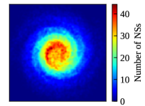
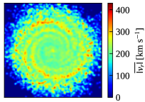
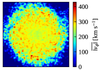
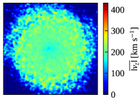
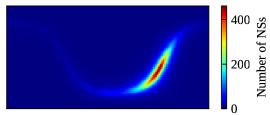
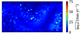
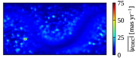
After the runs have been performed, we transform the output of the simulation into a representation that can be interpreted by a ML pipeline. Since ANNs require the use of structured data, we represent the position and velocity output of the simulations in the form of 2D binned density and velocity maps both in the galactocentric and ICRS reference frames. The density maps give information about the density of neutron stars in the Galaxy by providing the number count of stars in each spatial bin. On the other hand, velocity maps contain information about the kinematic properties of the neutron stars by providing the average magnitude of the stellar velocity components in each spatial bin. In the galactocentric maps the Galaxy is represented face on and projected onto the $xy$-plane of the Cartesian galactocentric frame, extending from $-20\,\mathrm{kpc}$ to $20\,\mathrm{kpc}$ in $x$ and $y$ direction. The ICRS maps instead extend from $0^{\circ}$ to $360^{\circ}$ in right ascension (RA) and from $-90^{\circ}$ to $90^{\circ}$ in declination (DEC). To each map we apply a smoothing Gaussian filter (with radius $4.0\cdot\sigma+0.5$ and $\sigma=1$) in order to add some blurring and avoid sharp features. By doing so, we reduce noisy high-frequency features and thus make the training more stable, presumably resulting in better generalization capabilities. Therefore, for each simulated population we have:

• 1 density map in the galactocentric frame.

• 3 velocity maps, one for each component of the velocity in cylindrical galactocentric coordinates $v_{r}$, $v_{\phi}$ and $v_{z}$ in [$\mathrm{km\,s^{-1}}$].

• 1 density map in ICRS coordinates.

• 2 proper motion maps, one for each component of the angular proper motion projected on the celestial sphere $\mu_{\rm RA}$ and $\mu_{\rm DEC}$ in [$\mathrm{mas\,yr^{-1}}$].

This set of maps for each population is labeled with the corresponding values of the parameters $\sigma_{\rm k}$ and $h_{\rm c}$ used to simulate that specific population.

We will test the ML performance on three different map resolutions. Thus, we generate each of the above data-sets with resolutions $32\times 32$, $128\times 128$ and $512\times 512$ square bins. Note that in the ICRS maps the DEC coordinate axis range is half that of the RA coordinate axis. Hence, these maps have half the bins along the DEC coordinate and their resolution is $32\times 16$, $128\times 64$ and $512\times 256$ square bins. For brevity hereafter we will refer to the three resolutions as 32, 128 and 512 resolutions for both galactocentric and ICRS maps, respectively. An example of the maps with resolution 128 for a simulation with fiducial values $h_{\rm c}=0.18\,\mathrm{kpc}$ and $\sigma_{\rm k}=265\,\mathrm{km\,s^{-1}}$ is shown in Figs. 1 and 2.

Before loading the maps into our ML pipeline, they are normalized so that each bin contains a continuous value between 0 and 1. The same applies to the related labels so that their values range continuously between 0 and 1. The aim of normalization is to speed up the training process and make convergence easier since all inputs will provide signals of similar magnitude to the loss-function minimization. This is useful especially for multi-parameter and multi-channel training, that is when we train a network to predict more than one parameter or use channels that have different absolute magnitudes. In these cases, training without normalization might lead to slower, worse or even no convergence at all. Apart from the blurring and normalization described above, we do not apply any additional pre-processing steps to our input data.

Figure 3: Schematic representation of our CNN architecture for an input of galactocentric maps with resolution $128\times 128$ and 4 channels (1 density map plus 3 velocity maps). A module formed by two blocks that each contain a convolution layer and max pooling layer is followed by a fully connected linear network with one hidden layer. The final network output is either a single parameter or two parameters depending on the experiment specifics.

3.2 Network Architecture

For the implementation of our ML pipeline we use PyTorch (Paszke et al., 2019), an optimized tensor library for deep learning using GPUs and CPUs, that is written in Python. The simplest neural network that can be used for this task is a fully connected neural network also referred to as a multi-layer perceptron (MLP) with only two layers of neurons, which are referred to as the input and output layer, respectively. As this is the starting point to develop more complicated and advanced architecture models, we first test how this simple configuration behaves. The number of neurons for the input layer is equal to the total number of input features, i.e., $C\times W\times H$. Here, $C$ is the number of input channels (corresponding to the total number of maps used), while $W$ and $H$ are the number of bins in width and height, respectively. The number of neurons in the output layer is equal to the number of regression parameters that we would like to predict, i.e., 1 or 2 in our experiments. For the activation function we use the Rectified Linear Unit (ReLU) defined as ${\rm ReLU}(x)=\max{(0,x)}$. To obtain the output values, the ReLU activation function is applied to a linear combination of the input features with weights and a bias.

A more sophisticated model architecture is represented by a convolutional neural network (CNN). CNNs are a particular type of deep neural network that have proven to be very successful in regression and classification tasks when applied to structured and matrix-like 2D inputs (see Rawat & Wang, 2017, for a review). The basic structure of CNNs consists of convolutional, pooling, and fully connected layers. Convolutional layers are multi-channel filters that slide along the 2D input maps and are able to extract feature maps. The role of the pooling layer is to down-sample the output of a convolutional layer. This inevitably causes a loss of information but in general helps to improve the training efficiency by increasing the size of the receptive field (i.e., the region of the input that produces the feature for each neuron) and reducing the number of trainable parameters. The fully connected layers collect all the output features from the convolution layers into a 1D input and return the final output prediction.

The detailed structure of the CNN we built for our case study can be found in Table 3. A schematic representation of its structure for a 4-channel input with galactocentric maps is also shown in Fig. 3 as an example. It consists of the following layers:

• A 2D convolution layer with kernel size $3\times 3$, $C$ input channels, 32 output channels, stride 1 and no padding.

• A 2D Max pooling layer of size $2\times 2$ with stride 2 and no padding.

• A 2D convolution filter with kernel size $3\times 3$, 32 input channels, 64 output channels, stride 1 and no padding.

• A 2D Max pooling layer of size $2\times 2$ with stride 2 and no padding.

• A fully connected linear layer with flattened input from the convolutional modules output and 64 output neurons.

• A fully connected linear layer with 64 input neurons and 1 or 2 output neurons (depending on the number of parameters we would like to predict).

For the convolutional and pooling layers the stride parameter regulates the amount of displacement in bins that the filter moves over the map at each step. Padding adds one or more bins at the border of the 2D maps, so that the filters can move and cover the whole map without leaving any bins out. We use a padding of 0 because the borders of the maps do not contain relevant information.

The choice of this architecture was found by trial and error experiments where we started from a very simple structure and progressively increased the complexity, adding more and more layers to acquire the desired accuracy in predicting the input parameters.

Table 3: CNN architecture. The total number of input and output features is reported. $C$ is the number of used channels, while $W$ and $H$ represent the number of bins (i.e. the resolution) in width and height of the density and velocity maps, respectively. Input and output feature numbers have been rounded down to the lower integer.

Layer	Input	Output
Conv2d + ReLU	$C\times W\times H$	$32\times(W-2)\times(H-2)$
MaxPool2d	$32\times(W-2)\times(H-2)$	$32\times\left(\frac{W}{2}-1\right)\times\left(\frac{H}{2}-1\right)$
Conv2d + ReLU	$32\times\left(\frac{W}{2}-1\right)\times\left(\frac{H}{2}-1\right)$	$64\times\left(\frac{W}{2}-3\right)\times\left(\frac{H}{2}-3\right)$
MaxPool2d	$64\times\left(\frac{W}{2}-3\right)\times\left(\frac{H}{2}-3\right)$	$64\times\left(\frac{W}{4}-\frac{3}{2}\right)\times\left(\frac{H}{4}-\frac{3}{2}\right)$
Linear + ReLU	$64\times\left(\frac{W}{4}-\frac{3}{2}\right)\times\left(\frac{H}{4}-\frac{3}{2}\right)$	64
Linear	64	1(2)

3.3 Training Process

For the training of the network, we use the root-mean-square error (RMSE) both for the loss function and validation metric, i.e., to compute the distance between the network predictions and the ground truths of the $h_{\rm c}$ and $\sigma_{\rm k}$ parameters. In general validation occurs at the same time as training and consists of testing the network over a data-set different from the training set. This is needed to asses the ability of the network to generalize what it is learning to an unknown data-set. The minimization of the loss function occurs through gradient descent and backpropagation (Kelley, 1960; Ruder, 2017), i.e., computation of the loss-function gradients with respect to all network parameters (weights and biases). These gradients taken with a negative sign indicate the directions towards which the network parameters should be updated so that the loss is reduced, and hence the network predictions move closer to the true, expected labels. In this regard, a crucial aspect to ensure the best performance of a neural network is to properly initialize the weights and biases. For this purpose we use the Kaiming initialization method (He et al., 2015) in order to avoid exploding or vanishing gradients during the training.

The training process itself is regulated by several hyperparameters. The first one is the learning rate, which is a coefficient for the weight updates. In general, a larger learning rate results in updates of larger magnitude, which could in turn lead to faster convergence, but might also reduce the stability of the training process and thus increase the risk of overshooting the minima of the loss landscape. A second hyperparameter is the batch size, which defines the number of samples that are packed together and passed through the network before an optimization step is performed. In general, for bigger training data-sets, a larger batch size helps to increase the efficiency and stability of the training process, since the gradient-descent steps are averaged over many samples and noise is reduced. For the gradient-descent optimizer we use the Adaptive Moment Estimation (Adam) (Kingma & Ba, 2014). As its name suggests, Adam adds an adaptive momentum term to the gradient descent to automatically modify the learning rate and accelerate convergence. When using the Adam optimizer the chosen initial value of the learning rate represents only an upper limit.

We fix the maximum number of learning epochs to 1024. Every epoch the network performs a series of optimization steps by going through the whole training data-set once. Then epoch-averaged loss and validation metric values are computed. If the validation metric value has improved with respect to the previous epoch the current status of the optimized network is saved. We set an early stop of 128 epochs, so that if the validation metric does not improve over this epoch span, the training process automatically stops and the weights of the best epoch are stored. This prevents the network from overfitting the training samples, which would reduce its ability to generalize over unknown data.

Figure 4: MLP best training RMSE values for the training process on the single parameter $\sigma_{\rm k}$ of the Maxwell kick-velocity distribution, as a function of the training data-set size and the resolution (red, blue, and orange curves for 32, 128 and 512 respectively) using the four different input configurations T1 (GC position), T2 (GC position + velocity), T3 (ICRS position) and T4 (ICRS position + velocity).

Figure 5: CNN best training RMSE values for the training process on the single parameter $\sigma_{\rm k}$ of the Maxwell kick-velocity distribution, as a function of the training data-set size and the resolution (red, blue, and orange curves for 32, 128 and 512 respectively) using the four different input configurations T1 (GC position), T2 (GC position + velocity), T3 (ICRS position) and T4 (ICRS position + velocity).

4 Experiments

As a first step we perform several tests to analyze which configuration of the input feature maps provides the best training experience and which proposed neural network architecture, either the MLP or the CNN, behaves better. Regarding the input configuration we would like to understand (i) what the best type of maps is (galactocentric vs equatorial ICRS); (ii) how many input channels are needed to obtain good results (do density maps provide enough information alone or does the addition of velocity maps improve the results?); (iii) which resolution of the input maps provides the best result. To do so, we first compare the behavior of the MLP and the CNN when trained to predict a single parameter. We explore different types of input signals by varying the resolution of the density and velocity maps as well as the number of input channels. Once we find the optimal configuration for the input maps and the best performing network, we proceed to test its generalization power. A similar strategy is then followed for the two-parameter prediction.

4.1 Single-parameter Predictions

4.1.1 Data-representation and Architecture Comparison

We focus on predicting the parameter $\sigma_{\rm k}$ of the Maxwell kick velocity function and employ the density and velocity maps generated from simulation run S1. We keep aside the data-set with 20000 samples as it will be used to asses the generalization power of the best performing network (see §4.1.2). Thus, we have training sets with increasing number of samples (from 4 to 1024) and increasing map resolution (32, 128, 512). For each of these training sets we compare the performance on four different kinds of input information:

• Galactocentric position information: 1 density map in galactocentric coordinates (1 channel).

• Galactocentric position and velocity information: 1 density map plus 3 velocity maps in galactocentric coordinates (4 channels).

• ICRS position information: 1 density map in equatorial ICRS coordinates (1 channel).

• ICRS position and velocity information: 1 density map plus 2 proper motion maps in equatorial ICRS coordinates (3 channels).

We fix the network architectures and the training set-up as described in §3.2 and §3.3. For these initial experiments we do not incorporate validation but only focus on the training results for different types of data-sets, as we are not yet interested in evaluating the generalization power of the networks. To assess the convergence of the training runs we set a threshold for the $\sigma_{\rm k}$ RMSE training loss to $10\,\mathrm{km\,s^{-1}}$. If the final RMSE value is higher than this threshold the training is repeated up to a maximum of 8 times. If convergence is not reached after 8 trials we take the trained model with the lowest final RMSE. For each training experiment we also monitor the computational time needed to perform a single optimization step on a single data batch (see Appendix B for more details).

Initially we perform a search for the starting value of the learning rate that provides the best results. In particular for the MLP we find that to ensure a decaying RMSE value during training, the initial learning rate needs to be decreased as the input-map resolution increases. Therefore, after several tests we set the initial learning rate to $10^{-4}$, $10^{-5}$ and $10^{-6}$, respectively, for the 32, 128 and 512 resolution maps. The CNN instead is more flexible and stable and all three initial learning rates are suitable for every resolution. In this case we set it to $10^{-4}$ to obtain training convergence in the smallest number of epochs.

Next, we tune the batch size to make the learning process more stable and efficient as the number of training samples increases. In general, we keep the batch size to 1 for the data-set sizes 4, 8, 16, 32 and progressively increase it to 4, 8, 16, 32, 64 as the data-set size increases to 64, 128, 256, 512, 1024, respectively. Only when testing the performance of the MLP on the T2 input configuration we need to further fine tune the batch size in order to reach acceptable values of the RMSE. In all other cases the batch sizes mentioned above work well.

Figure 6: Results of the CNN single-parameter prediction for the kick-velocity parameter $\sigma_{\rm k}$ and scale height $h_{\rm c}$ for the corresponding validation sets. Top (bottom) left panel: evolution of the RMSE training (red) and validation (blue) losses as a function of the training/validation epoch for the $\sigma_{\rm k}$ ($h_{\rm c}$) parameters. Top (bottom) central panel: residuals of the prediction as a function of the target $\sigma_{\rm k}$ ($h_{\rm c}$) value; the subscripts P and T refer to the predicted and target values, respectively. The red dashed lines delimit the $68$% uncertainty region corresponding to a RMSE $=4.4\,\mathrm{km\,s^{-1}}$ ($0.017\,\mathrm{kpc}$) computed over the whole range $[1,700]$ $\mathrm{km\,s^{-1}}$ ($[0.02,2]$ $\mathrm{kpc}$). The orange region delimits the $68$% uncertainty region computed as a running RMSE for which we have divided the full $\sigma_{\rm k}$ ($h_{\rm c}$) range into $50$ bins of equal size. The blue line shows the trend of the average residuals which are well centered around the value 0. Top (bottom) right panel: relative error of the prediction as a function of the target $\sigma_{\rm k}$ ($h_{\rm c}$) value. The red dashed line corresponds to a MRE $=0.014$ ($0.024$) computed over the whole range $[1,700]$ $\mathrm{km\,s^{-1}}$ ($[0.02,2]$ $\mathrm{kpc}$). The blue line shows the trend of the running MRE computed over $50$ bins of equal size into which we have divided the full $\sigma_{\rm k}$ ($h_{\rm c}$) range.

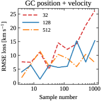
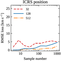
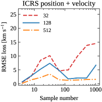
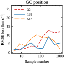
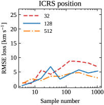
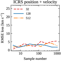
The results of our experiments using the MLP and the CNN on the training data-sets from S1 with configuration T1, T2, T3 and T4 are shown in Figs. 4 and 5, respectively (see Appendix B for the timing results), highlighting the best converged RMSE values as a function of the training data-set size and the resolution.

First of all, we note that for both model architectures, ICRS maps allow us to obtain slightly better results in terms of the best RMSE values. An explanation for this could be that only the ICRS maps contain 3D information of the Galaxy, i.e., they encode the stellar height distribution with respect to the galactic disk which correlates with the kick velocity magnitude. In fact the higher the kick velocity of newborn neutron stars the more spread out their distribution in galactic height $z$ at the end of the dynamical evolution. On the other hand galactocentric maps show the Galaxy represented face on and the information on the stars’ height $z$ with respect to the Galactic plane is hidden. Therefore, it is likely easier for the networks to distinguish populations with different $\sigma_{\rm k}$ by processing the ICRS maps.

We also note that the addition of the velocity or proper motion information has opposite effects on the two model architectures. In particular, on one side it worsens the MLP performance, as the best RMSE almost doubles. On the other side, it helps the CNN in reducing the overall RMSE. We interpret this as an indication that, as the complexity of the input data increases, a deeper (with more layers) and more sophisticated model architecture like the CNN is more suitable to process the input data and extract meaningful features to perform the regression task. However, the improvement is not dramatic, which could suggest that the density maps already provide enough information to distinguish, with sufficient precision, populations simulated with different $\sigma_{\rm k}$ values.

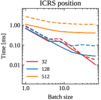
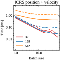
Concerning the resolution, we observe that higher resolutions allow us to reach slightly lower RMSE values with both the MLP and the CNN but at the expense of longer computation time (see Figs. 13 and 14 in Appendix B). We therefore consider the small differences between the best RMSE values obtained with 128 and 512 resolutions not sufficient to justify the choice of the higher resolution. Hence, the use of the 128 resolution appears to be a good compromise to ensure good accuracy and reasonably fast training.

In light of these results for the single-parameter estimation, we conclude that the optimal representation to be used for training is composed of the ICRS density plus proper motion maps with 128 resolution. Moreover, as the CNN obtains the best results and appears more stable and flexible when compared to the simple MLP (especially for the multi-channel input features), we employ our CNN architecture in the following experiments, which should also be less prone to overfitting.

4.1.2 Generalization Results

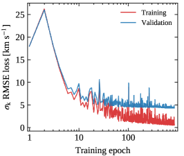
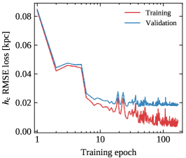
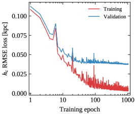
As the next step we separately train the CNN to predict the $\sigma_{\rm k}$ and $h_{\rm c}$ parameters by using the two big data-sets with 20000 simulations each (see S1 and S2). As input features we use the 3-channel ICRS representation with one density map and two proper motion maps with 128 resolution that ensure the best results as suggested by our earlier experiments. We randomly split both data-sets into training and validation subsets with a relative percentage of $80/20\%$, respectively. Therefore, training is performed over 16000 simulations, randomly sampled from the entire data-sets, while validation is performed over the remaining 4000 simulations. We adopt an initial learning rate of $10^{-4}$, a batch size of 64, set the total number of learning epochs to 1024 and an early stop at 128 epochs to avoid overfitting. The evolution of the training and validation losses is shown in the left panels of Fig. 6.

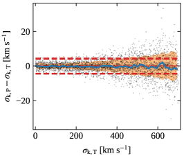
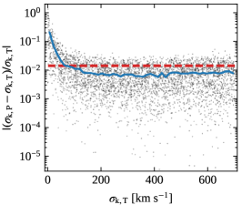
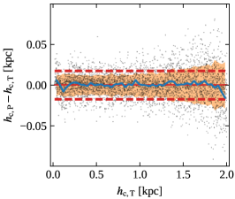
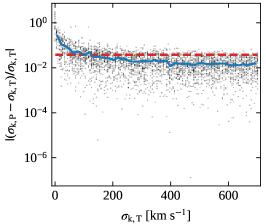
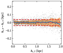
The predictions of the trained network on the validation set for $\sigma_{\rm k}$ and $h_{\rm c}$ are summarized in Fig. 6 and Table 4. In the first case, the network is able to predict the value of the kick-velocity parameter $\sigma_{\rm k}$ for the simulations in the validation data-set with a RMSE uncertainty of $4.4\,\mathrm{km\,s^{-1}}$, computed over the whole range $[1,700]$ $\mathrm{km\,s^{-1}}$. This is indicated by the red dashed lines in the residuals plot (see top central panel of Fig. 6), which delimit the $68$% uncertainty region. In the second case, the network is able to predict the value of the scale-height parameter $h_{\rm c}$ for the simulations in the validation data-set with a RMSE uncertainty of $0.017\,\mathrm{kpc}$, computed over the whole range $[0.02,2]$ $\mathrm{kpc}$ (see bottom central panel of Fig. 6). Note that in both experiments, the residuals spread out as the target values increase. We visualize this by computing a running RMSE with increasing target values. As is shown by the orange regions in the residuals plots, the running RMSE increases from $1.4$ to $7.1\,\mathrm{km\,s^{-1}}$ for $\sigma_{\rm k}$ and from $0.013$ to $0.028\,\mathrm{kpc}$ for $h_{\rm c}$, respectively. However, the average residuals are consistent with $0$ over the entire target value ranges as marked by the blue line in the residual plots, showing no anomalous trends in the predicted values.

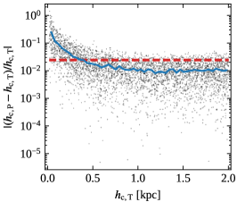
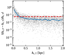
In the right panels of Fig. 6 we also show the relative error to highlight the precision with which the network is able to predict the $\sigma_{\rm k}$ and $h_{\rm c}$ parameters for a given target value. We observe that the precision of the predictions improves with increasing $\sigma_{\rm k}$ and $h_{\rm c}$ and eventually stabilizes to a relative error of around $0.01$. This is highlighted by the blue lines, which show the trend of the mean relative error (MRE) as a function of the target parameters. The red dashed lines correspond instead to the MRE computed on the whole parameter ranges and are equal to $0.014$ and $0.024$ for $\sigma_{\rm k}$ and $h_{\rm c}$, respectively. The fact that the precision of the predictions decreases at the lower end of the target ranges suggests that (for our chosen network set-up) the input maps become harder to distinguish as the neutron stars’ initial kick velocities and their galactic birth heights decrease in magnitude.

We then evaluate the generalization capability of the two trained networks on the corresponding test sets with 1000 samples each. We find RMSEs of $4.8\,\mathrm{km\,s^{-1}}$ and $0.019\,\mathrm{kpc}$ and MREs of $0.018$ and $0.029$ for $\sigma_{\rm k}$ and $h_{\rm c}$, respectively. To further assess the confidence intervals of both estimators, we evaluate the RMSE and the MRE of the parameter values predicted by the two networks over 1000 bootstrapped sets of the related test sets. We find that the RMSE variation is around $3$%, while the MRE variation is around $11$% for both predicted parameters. These results indicate that the trained networks are able to generalize well over unseen data-sets.

4.2 Two-parameter Predictions

4.2.1 Data-representation Comparison

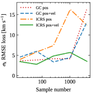
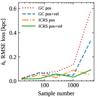
To see how the CNN behaves when two parameters, i.e., the kick-velocity parameter $\sigma_{\rm k}$ and the characteristic scale height $h_{\rm c}$, are inferred simultaneously, we use the data-set of maps generated from simulation run S3 (see §3.1). In this case, we have training sets with increasing number of samples, 16 = 4x4, 64 = 8x8, 256 = 16x16, 1024 = 32x32, 4096 = 64x64. We leave aside the largest data-set with 16384 = 128x128 simulations for our final generalization experiment. Given the results of the single-parameter training experiments, we choose the 128 resolution maps and compare the CNN’s performance on the four kinds of input information T1, T2, T3 and T4 as we did for the single-parameter case (see §4.1.1). We fix the CNN architecture and the training set-up as described in §3.2 and §3.3, respectively. As for the single-parameter comparison, we only focus on the training behavior for this initial comparison. We keep track of the RMSE training losses for both parameters separately, but training proceeds by minimizing the total loss computed on both parameters. We set the convergence threshold for $\sigma_{\rm k}$ to $10\,\mathrm{km\,s^{-1}}$ and for $h_{\rm c}$ to $0.5\,\mathrm{kpc}$; if convergence is not reached for both parameters after 8 training trials we quote the experiment with the best performance. As before, we also keep track of the computational time for a single optimization step (see Appendix B). The initial learning rate is set to $10^{-4}$, while the batch size is changed according to the data-set size. In particular, we use a batch size of 1, 4, 16, 64, 128 for the data-set sizes 16, 64, 256, 1024 and 4096, respectively.

The results of our experiments using the CNN for the two-parameter prediction on the training data-sets from S3, with configuration T1, T2, T3 and T4 are summarized in Fig. 7 (see Appendix B for the timing results). As in the single-parameter case we find that the best results are provided by the ICRS maps, which allow us to reach the lowest training RMSE losses for both parameters. In particular, for the ICRS 3-channel input, the CNN is able to reach a training RMSE loss $\lesssim 5\,\mathrm{km\,s^{-1}}$ for the $\sigma_{\rm k}$ parameter, comparable with the single-parameter case. For $h_{\rm c}$, the CNN reaches a training RMSE $\lesssim 0.1\,\mathrm{kpc}$. However, we note a drop in accuracy for the $\sigma_{\rm k}$ parameter when only the ICRS density maps are used. As already mentioned in §4.1.1, information on the stars’ $z$-coordinate is encoded in the ICRS maps. As we simultaneously vary the initial kick velocities and the galactic heights of the pulsars’ birth places, the degeneracy between the effects of these two parameters becomes relevant. This makes a distinction of the impact of one parameter over the other more difficult for the network, when only ICRS density maps are provided. Adding two extra channels that contain information about the stars’ proper motion thus helps to improve the accuracy on the kick-velocity parameter estimation. The results of these initial explorations are promising and indicate that our simple CNN architecture has good predictive power for both parameters, if provided with all three input channels in the ICRS representation.

Figure 7: CNN best training RMSE values for the training process on the two parameters $\sigma_{\rm k}$ of the Maxwell kick-velocity distribution (left panel) and characteristic scale height $h_{\rm c}$ (right panel) as a function of the training data-set size for the four different input configurations T1 (GC position), T2 (GC position + velocity), T3 (ICRS position) and T4 (ICRS position+ velocity).

Figure 8: Results of the CNN two-parameter prediction for the kick-velocity parameter $\sigma_{\rm k}$ and scale height $h_{\rm c}$ for the corresponding validation sets. Top (bottom) left panel: evolution of the RMSE training (red) and validation (blue) losses as a function of the training/validation epoch for the $\sigma_{\rm k}$ ($h_{\rm c}$) parameters. Top (bottom) central panel: residuals of the prediction as a function of the target $\sigma_{\rm k}$ ($h_{\rm c}$) value; the subscripts P and T refer to the predicted and target values, respectively. The red dashed lines delimit the $68$% uncertainty region corresponding to a RMSE $=8.8\,\mathrm{km\,s^{-1}}$ ($0.038\,\mathrm{kpc}$) computed over the whole range $[1,700]$ $\mathrm{km\,s^{-1}}$ ($[0.02,2]$ $\mathrm{kpc}$). The orange region delimits the $68$% uncertainty region computed as a running RMSE for which we have divided the full $\sigma_{\rm k}$ ($h_{\rm c}$) range into $50$ bins of equal size. The blue line shows the trend of the average residuals which are well centered around the value 0. Top (bottom) right panel: relative error of the prediction as a function of the target $\sigma_{\rm k}$ ($h_{\rm c}$) value. The red dashed line corresponds to a MRE $=0.039$ ($0.061$) computed over the whole range $[1,700]$ $\mathrm{km\,s^{-1}}$ ($[0.02,2]$ $\mathrm{kpc}$). The blue line shows the trend of the running MRE computed over $50$ bins of equal size into which we have divided the full $\sigma_{\rm k}$ ($h_{\rm c}$) range.

4.2.2 Generalization Results

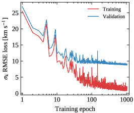
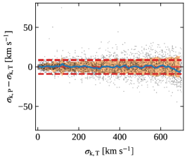
As for the single-parameter analysis, we assess the actual performance of the network when simultaneously predicting $\sigma_{\rm k}$ and $h_{\rm c}$ by training the CNN on the biggest data-set with $16384=128\times 128$ simulations (see run S3). As discussed above, we use the 3-channel ICRS representation with one density map and two proper motion maps with 128 resolution as input features. We split the entire data-set into training and validation subsets with a relative percentage of $80/20$%, respectively, leading to 13107 samples in the training and 3277 samples in the validation data-set and use the same configuration as in §4.1.2. The evolution of the individual training and validation losses is shown in the left panels of Fig. 8.

The results for the trained network’s prediction on the validation set for both parameters are shown in Fig. 8 and summarized in Table 4. The network is able to predict $\sigma_{\rm k}$ and $h_{\rm c}$ with an average RMSE uncertainty of $8.8\,\mathrm{km\,s^{-1}}$ and $0.038\,\mathrm{kpc}$, respectively, which is approximately doubled compared to the single-parameter experiment. These RMSE values are computed over the full target ranges and represented by the red dashed lines in the residuals plots (see central panels of Fig. 8). As in the single-parameter case, we observe that the RMSE uncertainties increase with increasing target parameters as indicated by the orange regions in the residuals plots. The relative errors represented in the right panels of Fig. 8 show the same decreasing trend with the target value as for the single-parameter predictions, albeit with larger relative errors. When computing the MRE over the whole range of the two target parameters, we obtain $0.039$ and $0.061$ for $\sigma_{\rm k}$ and $h_{\rm c}$, respectively. These values are highlighted by the red dashed lines in the right panels of Fig. 8.

We then evaluate the generalization capability of the trained network on the test set with 1000 samples. We find RMSEs of $9.1\,\mathrm{km\,s^{-1}}$ and $0.041\,\mathrm{kpc}$ and MREs of $0.041$ and $0.057$ for $\sigma_{\rm k}$ and $h_{\rm c}$, respectively. As before, we evaluate the confidence intervals of the two estimators over 1000 bootstrapped sets of the test set and find that the RMSE and MRE variations are around $3$% and $8$%, respectively, for both predicted parameters. This indicates that also in the two-parameter prediction the trained network is stable and guarantees a good level of generalization power.

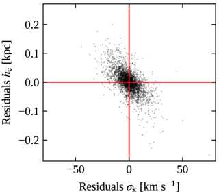
However, we find that the CNN trained to simultaneously predict $\sigma_{\rm k}$ and $h_{\rm c}$ is not able to reach the same level of accuracy as in the experiments where a single parameter was predicted at a time. This could be due to three distinct causes: (i) either our neural network is not sophisticated enough to discern between the effects of both parameters on the simulation outcomes represented in the ICRS maps, (ii) our choice of ICRS maps as input does not provide sufficient information for the network to distinguish between both parameters, or (iii) this is a physical (real) degeneracy, and there is a limit to what we can measure. To investigate this issue we train the CNN to predict only the parameter $h_{\rm c}$ using the same two-parameter data-set used above where both $\sigma_{\rm k}$ and $h_{\rm c}$ are varied. After predicting on the validation data-set we obtain a RMSE accuracy of $0.038\,\mathrm{kpc}$ which is equal to the result obtained above for the two-parameter prediction. This suggests that the network complexity is suitable to predict either one or two parameters simultaneously. Limitations in performance are therefore either due to an inadequate input representation or a physical degeneracy that imposes a natural accuracy threshold. While we cannot distinguish these two with our current simulation and ML pipeline, we can illustrate the underlying problem in the following way: Fig. 9 shows the residuals of the scale-height parameter $h_{\rm c}$ versus the residuals of the kick-velocity parameter $\sigma_{\rm k}$ for the predictions over the validation set. The overall negative slope indicates that the network tends to overpredict $h_{\rm c}$ in those simulations where $\sigma_{\rm k}$ is underestimated and vice versa; i.e., large (small) $h_{\rm c}$ values have the same overall effect on the phenomenology of the pulsar population as large (small) $\sigma_{\rm k}$ values and the network struggles to distinguish these cases. This highlights the degeneracy between the two parameters already discussed above, which might be broken if the data itself were represented in a different way or additional input information about each neutron star (beyond position and velocity) were provided.

Figure 9: Scatter plot of residuals of the predicted scale-height parameter $h_{\rm c}$ versus residuals of the predicted kick-velocity parameter $\sigma_{\rm k}$ for the validation data-set of our two-parameter generalization experiment. An anticorrelation can be observed.

Table 4: Summary of the CNN generalization results on the validation and test (in parenthesis) data-sets for the single-parameter and two-parameter cases.

	1-par. generalization		2-par. generalization
Parameter	RMSE	MRE	RMSE	MRE
$\sigma_{\rm k}$	$4.4\,(4.8)\,\mathrm{km~{}s^{-1}}$	0.014 (0.018)	$8.8\,(9.1)\,\mathrm{km~{}s^{-1}}$	0.039 (0.033)
$h_{\rm c}$	$0.017\,(0.019)\,\mathrm{kpc}$	0.024 (0.029)	$0.038\,(0.041)\,\mathrm{kpc}$	0.061 (0.057)

5 Discussion

In this paper we have studied the potential of an artificial neural network to estimate with high accuracy the dynamical characteristics of a mock population of isolated pulsars. Implementing a simplified population-synthesis framework we focused on the pulsar natal kick-velocity distribution and the distribution of birth distances from the Galactic plane. Taking into account the Galaxy gravitational potential and evolving the pulsar motions in time, we generate a series of simulations that are used to train and validate a suitably structured convolutional neural network.

The generalized results presented in the previous sections are obtained in a very idealized and simplified scenario, implying that caution is required when the uncertainties for the prediction of the kick-velocity dispersion $\sigma_{\rm k}$ and birth scale height $h_{\rm c}$ are taken at face value and conclusions for the real pulsar population are drawn.

Figure 10: Proper motions of the selected 216 neutron stars in the sky represented in the ICRS reference frame. The current locations of the neutron stars are indicated by the colored circles, whereas the tracks indicate their motion for the past $0.5\,\mathrm{Myr}$, assuming no radial velocity and neglecting the effects of the Galactic potential. The color encodes the heliocentric distance $d_{\odot}$ of the neutron stars. The corresponding data is provided in Table 5. In the background, we show in gray all non-binary pulsars in the ATNF catalogue (those in the Small and Large Magellanic Clouds as well as those in globular clusters are included). The red star highlights the position of the Galactic Center.

In particular, our simulations assume that the distribution of neutron star progenitors in Galactic height is represented by the exponential thin-disk model, and that the kick-velocity magnitudes follow a Maxwellian distribution. While the choice of an exponentially thin disk is commonly adopted (Wainscoat et al., 1992; Polido et al., 2013; Li et al., 2019) and can be justified theoretically as the outcome of a self-gravitating isothermal disk (Spitzer, 1942), the choice of a Maxwellian model for the kick-velocity distribution is difficult to motivate from a theoretical standpoint. The Maxwellian model has found empirical support as it has been shown to well describe the proper motions of observed pulsars (Hobbs et al., 2005). It is for this reason, and its rather simple mathematical form, that the Maxwell kick-velocity distribution is often adopted in population synthesis studies of compact stars (Sartore et al., 2010; Cieślar et al., 2020). However, the real functional form of the kick-velocity distribution is still unknown and debated. Several authors have studied the kick-velocity problem and concluded that other models explain observed proper motions of neutron stars equally well. For example, by using maximum-likelihood methods Arzoumanian et al. (2002) found that a bimodal Gaussian distribution with a low-velocity and a high-velocity component is the preferred model to describe the observed proper motion of a sample of 79 radio pulsars. Faucher-Giguère & Kaspi (2006) studied the velocity component along the Galactic longitude for a sample of 34 pulsars observed with interferometric techniques (Brisken et al., 2002, 2003). After testing a two-component Gaussian model as well as a variety of single-component models, they opted for a single-component description with an exponential shape, although a two-component model could not be ruled out due to the poor statistics of their sample. More recently, Verbunt et al. (2017) and Igoshev (2020) analyzed a sample of isolated young pulsars and found that a two-component Maxwellian model explained the observed sample best.

In general, the presence of a low-velocity and a high-velocity component could indicate different progenitor properties as well as birth scenarios for the pulsar population. Numerical simulations of supernova explosions have for example suggested that neutron stars with lower kick velocities could be generated in the core-collapse supernovae of progenitors with small iron cores or in electron-capture supernovae (Podsiadlowski et al., 2004; Mandel & Müller, 2020). While also possible scenarios for isolated systems (Janka, 2017), such conditions might generally affect those neutron stars born in binaries (Giacobbo & Mapelli, 2020), where mass-loss episodes could strip their progenitors off their hydrogen envelopes. This might favor the formation of small iron cores or accretion-induced electron-capture supernovae, resulting in weaker natal kicks (Schwab et al., 2010; Tauris et al., 2013). Only for the strongest kicks can the binaries be disrupted by the supernova and both companions expelled; otherwise the two stars remain gravitationally bound. Such effects are neglected in our model but could in principle generate an imprint on the observed neutron star population. The ability of ML algorithms to recognize features and patterns in the processed data could help to better constrain the bi-modality of the kick-velocity distribution. In future work, we will investigate these aspects in more detail and explore ways to implement a ML framework to reconstruct the shape of the kick-velocity distribution underlying an evolved population of pulsars.

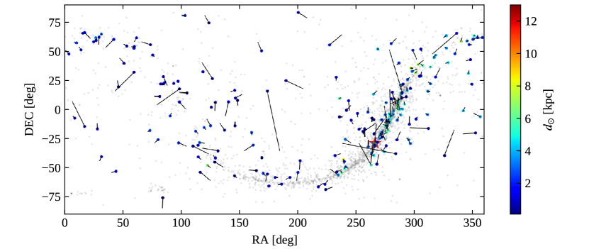
Up to this point, we have not considered any kind of selection effects or observational biases and effectively assumed that all the neutron stars in our simulation are detectable. While this provides direct insight into how various initial conditions affect the evolved population of neutron stars, a direct comparison with observational data in principle requires a careful treatment of biases. For example, due to beaming effects not all Galactic radio pulsars are visible from Earth (Tauris & Manchester, 1998; Melrose, 2017), while survey sensitivity thresholds and instrumental limitations might hamper the detection of faint or far away sources (Manchester et al., 2001; Johnston et al., 2008; Stovall et al., 2014; Coenen et al., 2014; Good et al., 2020). Additionally, timing noise can significantly limit the sensitivity and precision in the detection of pulsar proper motions via timing analysis techniques (Hobbs et al., 2004; Lentati et al., 2016; Parthasarathy et al., 2019). With the aim of obtaining a rough idea on how selection effects and biases could potentially influence a future comparison with observational we perform the following experiment. We first collect those neutron stars that have measured proper motions. As the main resource we use the ATNF pulsar catalogue (Manchester et al., 2005), but in some cases we provide proper motion results from more recent analyses (see Appendix C for details). We find a total of 417 neutron stars whose angular positions, proper motions in ICRS coordinates, spin periods, spin-period derivatives, $DM$ values and distance estimates are reported in Table 5. Out of these objects, we remove those stars that belong to the Magellanic Clouds, are associated with globular clusters or have a binary companion. We further select only those neutron stars with a spin-period derivative $\dot{P}>10^{-17}$ to exclude those that have potentially been recycled. Finally, we consider only those for which an estimate of the heliocentric distance $d_{\odot}$ is available; in the case of radio pulsars we quote values that are derived from their respective $DM$s using the free-electron density model of Yao et al. (2017) (YMW16 model hereafter). As some neutron stars have a $DM$ that exceeds the maximum Galactic $DM$ allowed by the YMW16 model, these cases are assigned a default distance of $25\,\mathrm{kpc}$. We exclude those cases unless an alternative distance measurement is available. Applying these filters we obtain a sample of 216 Galactic, likely isolated neutron stars, whose positions and proper motions are illustrated in Fig. 10.

Figure 11: Distribution of heliocentric distances $d_{\odot}$ (left panel) and proper-motion magnitudes $\mu_{\rm tot}$ (right panel) for the 216 neutron stars with measured proper motion (gray histograms). For comparison, we also show the distances and proper-motion magnitudes for 216 simulated neutron stars (blue histograms) randomly sampled from a mock population generated with the fiducial parameters $\sigma_{\rm k}=265\,\mathrm{km\,s^{-1}}$ and $h_{\rm c}=0.18\,\mathrm{kpc}$ (red histograms). For the weighted sampling, we use the weight function $f(d_{\odot})=d_{\odot}^{-1}\exp(-0.5d_{\odot})$.

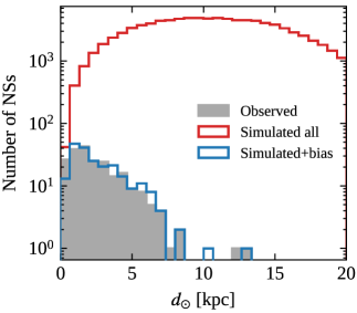
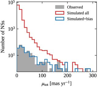
In the left panel of Fig. 11, the gray histogram shows the distribution of their heliocentric distances. Even if subject to some uncertainties due to imprecisions in the YMW16 model, the distance distribution peaks around $1\,\mathrm{kpc}$, followed by a sharp exponential decrease. For a realistic pulsar distribution and in the absence of selection effects, we would expect the number of neutron stars to increase with distance due to an increase in the explored volume, until reaching a maximum at a distance of about $10\,\mathrm{kpc}$, which comprises the region around the Galactic Center (see the red histogram in the left panel of Fig. 11). Thus, the shape of the gray distribution in Fig. 11, as expected, indicates that our observed sample of neutron stars with measured proper motions is incomplete in distance and subject to selection biases. By looking at the right panel of Fig. 11, we also note that a selection bias on distance is also reflected in the distribution of the total proper motion magnitudes (gray histogram), computed as $\mu_{\rm tot}\equiv\sqrt{\mu_{\rm RA}^{2}+\mu_{\rm DEC}^{2}}$. Indeed, since the nearest stars are also characterized by larger angular proper motions, there is a tendency to detect high proper-motion stars with higher probability.

In this first empirical approach, instead of attempting to identify these underlying biases (which will be the subject of a subsequent paper in preparation), we follow a more agnostic approach to introduce a comparable selection effect in our simulated populations. Specifically, we use a weighted random-sampling routine to select $n$ pulsars from our mock populations, where each simulated star is assigned a weight according to a function $f(d_{\odot})$ of its heliocentric distance. This weight function has to assign larger weights to closer neutron stars in order to ensure their higher detection probabilities and has to be chosen such that we recover the observed distance distribution with sufficient accuracy. To find $f(d_{\odot})$ we simulate a mock population with the fiducial values of the kick velocity and scale height, that is $\sigma_{\rm k}=265\,\mathrm{km\,s^{-1}}$ and $h_{\rm c}=0.18\,\mathrm{kpc}$, respectively. After using a given $f(d_{\odot})$ to weight the simulated neutron stars we sample 216 mock stars and compare their distance and proper-motion distributions (shown as blue histograms in Fig. 11) with those of the observed sample by performing two-sample Kolmogorov-Smirnov (KS) tests. After testing various functional forms we find that $f(d_{\odot})=d_{\odot}^{-1}\exp(-0.5d_{\odot})$ is able to reproduce the observed distributions with a good level of accuracy. More precisely, for this choice of $f(d_{\odot})$, the KS tests performed over $1000$ distinct comparisons give average p-values of $\sim 0.3$ and $\sim 0.6$ for the distance and proper-motion comparison, respectively. This means that at $95$% confidence level, we cannot reject the null hypothesis that the simulated and observed samples are drawn from the same underline distribution. We have also verified that for this weight function, the KS tests always provide p-values $>0.05$ when comparing the observed sample with the simulated populations for reasonable values of $\sigma_{\rm k}$ and $h_{\rm c}$. Only in the cases where $\sigma_{\rm k}$ and $h_{\rm c}$ assume extreme values (near the edges of their respective ranges) the p-values might drop below $0.05$. However, these cases are associated with simulations with extreme initial conditions that are unlikely to reproduce the observations. For our basic experiment, we further make the simplified assumptions that $f(d_{\odot})$ emulates all selection biases and that it is the same for every number $n$ of sampled neutron stars. We stress that for the purpose of this initial analysis we do not aim to accurately constrain the selection function that affects the observed population of neutron stars. Instead we study how the introduction of realistic selection biases will alter the predictive power of our machine learning framework. Although one might intuitively attribute the exponential factor in $f(d_{\odot})$ to scattering in the interstellar medium at large distances, the underlying nature and the precise form of the true selection function is certainly more complicated. We expect it to encompass a series of effects due to the physics of the interstellar medium and the pulsar emission itself, as well as selection effects of pulsar surveys and pulsar searches. We reserve a more accurate study disentangling the different effects that contribute to $f(d_{\odot})$ to future work.

We then analyze how the predictive power of the CNN evolves as a function of the number $n$ of neutron stars, sampled with the above weight function $f(d_{\odot})$. To do so, we vary $n$ from 200 to 2000 in steps of 200, and in each case re-sample the 16384 simulated populations from run S3, where both $\sigma_{\rm k}$ and $h_{\rm c}$ are varied. After applying a $80/20$% training-validation split, we retrain the CNN on each of the down-sampled simulations. As before, we use the 3-channel ICRS input maps (i.e., density plus proper motion information) but instead opt for a resolution of $32\times 16$ bins to accommodate the smaller number of stars represented in our maps. We have verified that a higher resolution of $128\times 64$ bins does not affect the training results significantly, but slows down the training process; we therefore choose the lower resolution. We use the same training hyperparameters as in §4.1.2, that is an initial learning rate of $10^{-4}$, a batch size of 64 and an early stop at 128 epochs. Once trained for each $n$ value, we apply the CNN to the validation sets and compute the root-mean-square error (RMSE) and mean relative error (MRE) for the $\sigma_{\rm k}$ and $h_{\rm c}$ predictions as a function of $n$.

In the left panel of Fig. 12, we show how the RMSE uncertainties for the predictions of the two parameters $\sigma_{\rm k}$ (blue) and $h_{\rm c}$ (red) diminish with increasing number of neutron stars $n$ sampled from the simulations. We observe that both curves (with the appropriate rescaling) follow very similar trends. On the right, we show instead how the MREs evolve with $n$, indicating how the precision of the two-parameter prediction improves with the number of detected neutron stars. This plot shows that, under the assumptions that selection effects are unaltered and the underlying kick-velocity and birth-height distributions have a Maxwellian and exponential shape, respectively, our trained CNN is able to predict $\sigma_{\rm k}$ and $h_{\rm c}$ with a relative error of $\sim 0.35$ for a sample of 2000 stars.

Figure 12: Trend of the RMSE (left panel) and MRE (right panel) uncertainties on the prediction of the two parameters $\sigma_{\rm k}$ (blue) and $h_{\rm c}$ (red) as a function of the number of neutron stars $n$ in the resampled simulations in the validation sets. To train and validate the CNN we use the 16384 simulated populations from simulation run S3 (with a $80/20$% training/validation split), where both $\sigma_{\rm k}$ and $h_{\rm c}$ are varied, and which are resampled with increasing number of stars $n$ according to the weight function $f(d_{\odot})=d_{\odot}^{-1}\exp(-0.5d_{\odot})$.

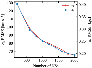
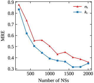
These results highlight that the number of neutron stars plays a crucial role for the level of accuracy that the CNN can reach. As expected, a larger number of stars provides more information, which allows the CNN to pinpoint differences between populations evolved from different initial conditions, also when selection effects are introduced. Future observational efforts aimed at detecting and characterizing new pulsars will thus play an important role in constraining the birth properties of neutron stars. Specifically, the advent of the Square Kilometer Array (SKA) will represent an important step forward into this direction. Due to its large sensitivity (a factor of 10 better than other radio telescopes) and its long baseline (up to $3000\,\mathrm{km}$), SKA has the potential to increase the number of discovered pulsars by a factor $10$ (Smits et al., 2009, 2011). This will allow more precise timing and astrometric measurements of pulsar positions as well as distances and proper motions. A larger and more precise data-set could also help to better constrain the shape of the kick-velocity distribution and differentiate between models that try to explain the origin of the natal kicks (Tauris et al., 2015).

6 Summary

In this work we have analyzed the possibility of using machine-learning (ML) techniques to reconstruct the dynamical birth properties of an evolved population of isolated neutron stars. For this purpose, we developed a simplistic population-synthesis pipeline to simulate the dynamical evolution of Galactic neutron stars and subsequently used these simulations to train and validate two different neural networks. We specifically focused on their ability to predict two parameters that strongly impact on the phenomenology of the evolved population: the dispersion $\sigma_{\rm k}$ of a Maxwell kick-velocity distribution and the scale height $h_{\rm c}$ of an exponential distribution for the Galactic birth heights. This was achieved by providing the networks with two-dimensional stellar density and velocity maps in galactocentric and equatorial (ICRS) coordinate frames. We found that a convolutional neural network (CNN) is able to estimate the physical parameters with high accuracy when multiple input channels, i.e., position and velocity information, are provided. In particular, when simultaneously predicting $\sigma_{\rm k}$ and $h_{\rm c}$ from ICRS maps, the network is able to reach absolute uncertainties lower than $10\,\mathrm{km\,s^{-1}}$ and $0.05\,\mathrm{kpc}$, respectively, corresponding to a relative error of around $10^{-2}$ for both parameters. Albeit obtained under simplified assumptions, our feasibility study, the main focus of this paper, has thus demonstrated that ML techniques are indeed suitable to infer information about the pulsar population. Our phenomenological analysis incorporating proper-motion measurements (an attempt at including observational biases in an agnostic way) has further highlighted that increasing the sample of known pulsars and accurately measuring their current characteristics with future telescopes is crucial to tightly constrain the birth properties of the neutron stars in the Milky Way. In particular, our trained CNN is able to predict $\sigma_{\rm k}$ and $h_{\rm c}$ with a relative error of $\sim 0.35$ for a sample of 2000 pulsars with measured proper motions.

We also demonstrated that one of the main factors in limiting the accuracy of the CNN’s predictions in our set-up is the degeneracy between $\sigma_{\rm k}$ and $h_{\rm c}$; as they both affect the evolved populations in a similar way, the network struggles to disentangle their effects. This limitation is a direct consequence of our simplified population-synthesis framework. In future works, we will go beyond modeling the dynamical evolution and focus on incorporating additional physics such as magneto-thermal and spin-period evolution. We will further model their emission in different electromagnetic bands and study corresponding detectability limits by addressing selection effects as well as observational survey biases. Such additional input information could potentially break the degeneracy between the kick-velocity and the Galactic height distributions and provide more accurate model constraints on $\sigma_{\rm k}$ and $h_{\rm c}$ as well as other input parameters.

The ultimate goal will be to use multi-wavelength observations of the Galactic neutron star population and take advantage of ML, combined with population synthesis, to recover their birth properties, such as the natal kick-velocity, spin-period or magnetic-field distribution. The potential to learn complex patterns from multi-dimensional data and the power of generalizing to unseen data-sets, makes ML algorithms a powerful tool to tackle such multi-parameter optimization studies.

Appendix A Hardware and Software

Our test machine features an Intel(R) Xeon(R) Gold 6230R CPU at 2.10GHz with a single NVIDIA GTX 2080 Ti GPU, 16 GiB RAM, and SSD drives. The system is running CentOS Linux release 7.8.2003 (Core) with PyTorch 1.2.0, CUDA toolkit 10.0.130 and GPU driver 455.32.00.

Figure 13: MLP forward (solid lines) and backward (dashed lines) pass times per sample in ms for the training process on the single parameter $\sigma_{\rm k}$ of the Maxwell kick-velocity distribution, as a function of the batch size and the resolution (red, blue, and orange curves for 32, 128 and 512 respectively) using the four different input configurations T1 (GC position), T2 (GC position + velocity), T3 (ICRS position) and T4 (ICRS position + velocity).

Figure 14: CNN forward (solid lines) and backward (dashed lines) pass times per sample in ms for the training process on the single parameter $\sigma_{\rm k}$ of the Maxwell kick-velocity distribution, as a function of the batch size and the resolution (red, blue, and orange curves for 32, 128 and 512 respectively) using the four different input configurations T1 (GC position), T2 (GC position + velocity), T3 (ICRS position) and T4 (ICRS position + velocity).

Appendix B Timing Tests

B.1 Timing for Single-parameter Predictions

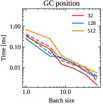
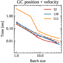
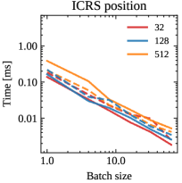
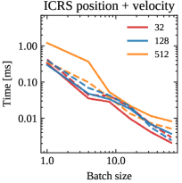
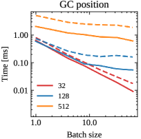
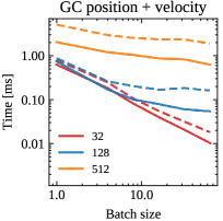
We report here the timing benchmarks for the MLP and CNN during the single-parameter training experiments discussed in §4.1.1. We run our experiments on the test machine and individually record the forward pass time (the time needed to go through the samples in a batch and compute a prediction) and the backward pass time (the time to compute all the gradients and perform a single optimization step) as a function of the batch size and resolution. Our benchmarks for the training data-sets from simulation run S1 using the four training configurations T1, T2, T3 and T4 are shown in Figs. 13 and 14, respectively.

The timing benchmark shows that the MLP is slightly faster in performing an optimization step. This is expected due to fewer trainable parameters when compared to the more complex CNN. We can also see that the forward and backward pass times per sample decrease with increasing batch size for both the MLP and CNN. For a larger batch size, several input samples are transferred from the CPU to the GPU in one step, reducing the overall number of calls between the two. Thus, on average, the processing time for an individual sample reduces when the batch size is increased. Moreover, a higher resolution generally implies an increase in computational cost, albeit being more pronounced in the case of the CNN than the MLP. The number of input channels itself has very little effect on our timings. Finally, we note that ICRS maps are slightly faster to process (in particular for the higher resolutions), due to the fact that their size is smaller compared to the galactocentric maps (they have half the height in bins).

B.2 Timing for Two-parameter Predictions

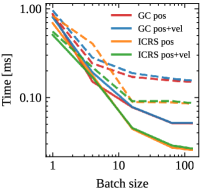
Following the results for the single-parameter experiments, we restrict our two-parameter predictions to the CNN model only and fix the resolution of the input maps to 128. The results of our timing benchmarks using the training data-sets from simulation run S3 with the four configurations T1, T2, T3 and T4 are shown in Fig. 15. We again report the timings for the forward and backward passes per sample as a function of the batch size and the type of input channels provided. As for the single-parameter case, we conclude that using ICRS maps ensures the lowest forward and backward pass times.

Figure 15: CNN forward pass (solid line) and backward pass time (dashed line) per sample for the two-parameter experiments as a function of the batch size for the four different input configurations T1 (GC position), T2 (GC position + velocity), T3 (ICRS position) and T4 (ICRS position + velocity).

Appendix C Neutron stars with measured proper motion

In Table 5, we report the properties of 417 neutron stars with measured proper motions in RA and DEC. Data for these neutron stars are primarily collected from the ATNF catalogue (Manchester et al., 2005). In some cases, updated estimates are available and those values quoted and the corresponding references specified. Note that in those cases, where multiple proper-motion estimates are available, we choose the ones with the lowest absolute error. The columns report in order: (i) the object name based on J2000 coordinates; (ii) the right ascension (RA) in hour angle and (iii) declination (DEC) in degrees with the last digit uncertainty given in parentheses; the proper motion in (iv) RA and (v) DEC in milliarcseconds per year with corresponding uncertainties; (vi) the parallax measured in milliarcseconds with uncertainty where available; (vii) the position epoch in modified Julian days; (viii) the spin period in seconds; (ix) the spin-period derivative in seconds over seconds; (x) the dispersion measure in $\mathrm{[pc\,cm^{-3}}]$ with the last digit uncertainty given in parentheses; (xi) the heliocentric distance derived from the $DM$ using the YMW16 free-electron density model (for some objects the $DM$ exceeds the maximum Galactic $DM$ allowed by the YMW16 model, which assigns a default value of $25\,\mathrm{kpc}$; when available, we quote other distance estimates; * indicates a distance derived from other techniques especially for X-rays and gamma-ray sources, which have no measured $DM$); (xii) the classification of the object, i.e., radio pulsar (PSR), binary pulsar (binary PSR), gamma-/X-ray pulsar (Gamma-/X-ray PSR), magnetar (MAG), X-ray dim isolated neutron star (XDINS); if the object is associated with a globular cluster (GC) or the Small Magellanic Cloud (SMC) this is reported in brackets; and (xiii) the reference for the proper motion measurements, indicated only if different from the ATNF catalogue, i.e., [1] Motch et al. (2009), [2] Eisenbeiss et al. (2010), [3] Walter et al. (2010), [4] Stovall et al. (2014), [5] Jennings et al. (2018), [6] Perera et al. (2019), [7] Dang et al. (2020), [8] Danilenko et al. (2020).

=9mm

Table 5: Up-to-date list of 417 neutron stars with measured proper motions in RA and DEC.

JName	RA	DEC	$\mu_{\rm RA}$	$\mu_{\rm DEC}$	parallax	Pos. Epoch	$P$	$\dot{P}$	$DM$	$d_{\odot}$	Class(Assoc.)	Ref.
	[hms]	[∘ ’ ”]	[mas yr-1]	[mas yr-1]	[mas]	[MJD]	[s]	[s s-1]	[pc cm-3]	[kpc]
J0014+4746	00:14:17.75(4)	+47:46:33.4(3)	$19.3\pm 1.8$	$-19.7\pm 1.5$	$\_$	49664	$1.24070$	$5.6446\times 10^{-16}$	$30.405(13)$	1.776	PSR
J0023+0923	00:23:16.87910(2)	+09:23:23.8689(8)	$-12.4\pm 0.5$	$-6.1\pm 0.1$	$0.4\pm 0.3$	56567	$0.00305$	$1.14234\times 10^{-20}$	$14.32810(4)$	1.248	PSR	[6]
J0024-7204ab	00:24:08.1615(5)	-72:04:47.602(2)	$4.2\pm 0.6$	$-2.9\pm 0.5$	$\_$	51600	$0.00370$	$9.820\times 10^{-21}$	$24.37(2)$	2.54	PSR(GC)
J0024-7204C	00:23:50.3546(1)	-72:04:31.5048(4)	$5.2\pm 0.1$	$-3.1\pm 0.1$	$\_$	51600	$0.00576$	$-4.98503\times 10^{-20}$	$24.5955(8)$	2.594	PSR(GC)
J0024-7204D	00:24:13.88092(6)	-72:04:43.8524(2)	$4.24\pm 0.07$	$-2.24\pm 0.05$	$\_$	51600	$0.00536$	$-3.4220\times 10^{-21}$	$24.7432(9)$	2.631	PSR(GC)
J0024-7204E	00:24:11.10528(5)	-72:05:20.1492(2)	$6.15\pm 0.03$	$-2.35\pm 0.06$	$\_$	51600	$0.00354$	$9.85103\times 10^{-20}$	$24.236(2)$	2.509	PSR(GC)
J0024-7204F	00:24:03.85547(10)	-72:04:42.8183(2)	$4.52\pm 0.08$	$-2.5\pm 0.05$	$\_$	51600	$0.00262$	$6.45029\times 10^{-20}$	$24.382(5)$	2.543	PSR(GC)
J0024-7204G	00:24:07.9603(1)	-72:04:39.7030(5)	$4.5\pm 0.1$	$-2.9\pm 0.1$	$\_$	51600	$0.00404$	$-4.21584\times 10^{-20}$	$24.436(4)$	2.556	PSR(GC)
J0024-7204H	00:24:06.7032(2)	-72:04:06.8067(6)	$5.1\pm 0.2$	$-2.8\pm 0.2$	$\_$	51600	$0.00321$	$-1.8294\times 10^{-21}$	$24.369(8)$	2.541	PSR(GC)
J0024-7204I	00:24:07.9347(2)	-72:04:39.6815(7)	$5\pm 0.2$	$-2.1\pm 0.2$	$\_$	51600	$0.00348$	$-4.5874\times 10^{-20}$	$24.43(1)$	2.555	PSR(GC)
J0024-7204J	00:23:59.4077(1)	-72:03:58.7908(5)	$5.27\pm 0.06$	$-3.59\pm 0.09$	$\_$	51600	$0.00210$	$-9.7917\times 10^{-21}$	$24.5932(1)$	2.594	PSR(GC)
J0024-7204L	00:24:03.7721(3)	-72:04:56.923(2)	$4.4\pm 0.2$	$-2.4\pm 0.2$	$\_$	51600	$0.00435$	$-1.22045\times 10^{-19}$	$24.40(1)$	2.547	PSR(GC)
J0024-7204M	00:23:54.4899(3)	-72:05:30.756(2)	$5\pm 0.3$	$-2\pm 0.4$	$\_$	51600	$0.00368$	$-3.8419\times 10^{-20}$	$24.43(2)$	2.553	PSR(GC)
J0024-7204N	00:24:09.1880(2)	-72:04:28.8907(7)	$6.3\pm 0.2$	$-2.8\pm 0.2$	$\_$	51600	$0.00305$	$-2.18570\times 10^{-20}$	$24.574(9)$	2.589	PSR(GC)
J0024-7204O	00:24:04.65254(6)	-72:04:53.7670(2)	$5.01\pm 0.05$	$-2.58\pm 0.08$	$\_$	51600	$0.00264$	$3.03493\times 10^{-20}$	$24.356(2)$	2.537	PSR(GC)
J0024-7204Q	00:24:16.4909(1)	-72:04:25.1644(6)	$5.2\pm 0.1$	$-2.6\pm 0.1$	$\_$	51600	$0.00403$	$3.4008\times 10^{-20}$	$24.265(4)$	2.517	PSR(GC)
J0024-7204R	00:24:07.5851(2)	-72:04:50.3954(5)	$4.8\pm 0.1$	$-3.3\pm 0.2$	$\_$	51600	$0.00348$	$1.48352\times 10^{-19}$	$24.361(7)$	2.538	PSR(GC)
J0024-7204S	00:24:03.9794(1)	-72:04:42.3530(4)	$4.5\pm 0.1$	$-2.5\pm 0.1$	$\_$	51600	$0.00283$	$-1.205413\times 10^{-19}$	$24.376(4)$	2.542	PSR(GC)
J0024-7204T	00:24:08.5491(5)	-72:04:38.932(3)	$5.1\pm 0.6$	$-2.6\pm 0.7$	$\_$	51600	$0.00759$	$2.93805\times 10^{-19}$	$24.41(2)$	2.55	PSR(GC)
J0024-7204U	00:24:09.8366(1)	-72:03:59.6882(4)	$4.6\pm 0.2$	$-3.8\pm 0.1$	$\_$	51600	$0.00434$	$9.52279\times 10^{-20}$	$24.337(4)$	2.534	PSR(GC)
J0024-7204W	00:24:06.058(1)	-72:04:49.088(2)	$6.1\pm 0.5$	$-2.6\pm 0.3$	$\_$	50000	$0.00235$	$-8.65526\times 10^{-20}$	$24.367(3)$	2.539	PSR(GC)
J0024-7204X	00:24:22.38565(9)	-72:01:17.4414(7)	$5.8\pm 0.1$	$-3.3\pm 0.2$	$\_$	54000	$0.00477$	$1.83610\times 10^{-20}$	$24.539(5)$	2.587	PSR(GC)
J0024-7204Y	00:24:01.4026(1)	-72:04:41.8363(4)	$4.4\pm 0.1$	$-3.4\pm 0.1$	$\_$	51600	$0.00220$	$-3.51721\times 10^{-20}$	$24.468(4)$	2.563	PSR(GC)
J0024-7204Z	00:24:06.041(2)	-72:05:01.480(6)	$4\pm 2$	$1\pm 2$	$\_$	51600	$0.00455$	$-4.54\times 10^{-21}$	$24.45(4)$	2.559	PSR(GC)
J0030+0451	00:30:27.42838(3)	+04:51:39.707(1)	$-6.4\pm 0.1$	$0.9\pm 0.3$	$2.94\pm 0.09$	55390	$0.00487$	$1.01743\times 10^{-20}$	$4.33991(7)$	0.345	PSR	[6]
J0034-0534	00:34:21.83422(8)	-05:34:36.722(3)	$7.9\pm 0.3$	$-9.2\pm 0.6$	$\_$	55000	$0.00188$	$4.966\times 10^{-21}$	$13.76517(4)$	1.348	PSR	[6]
J0034-0721	00:34:08.8703(1)	-07:21:53.409(2)	$10.37\pm 0.08$	$-11.13\pm 0.16$	$0.93\pm 0.08$	52275	$0.94295$	$4.08210\times 10^{-16}$	$10.922(6)$	0.996	PSR
J0040+5716	00:40:32.3899(1)	+57:16:24.833(1)	$12.39\pm 0.05$	$-5.4\pm 0.1$	$0.11\pm 0.04$	49667	$1.11823$	$2.878973\times 10^{-15}$	$92.5146(25)$	2.42	PSR
J0045-7319	00:45:35.255(10)	-73:19:03.32(1)	$0.31\pm 0.11$	$-0.931\pm 0.099$	$0.04\pm 0.06$	57205.875	$0.92628$	$4.4632\times 10^{-15}$	$105.4(7)$	58.725	Binary PSR(SMC)	[5]
J0055+5117	00:55:45.3981(1)	+51:17:24.601(1)	$10.47\pm 0.07$	$-17.4\pm 0.1$	$0.35\pm 0.06$	49664	$2.11517$	$9.53764\times 10^{-15}$	$44.0127(24)$	1.935	PSR
J0101-6422	01:01:11.1163(2)	-64:22:30.171(2)	$10\pm 1$	$-12\pm 2$	$\_$	55520	$0.00257$	$5.16\times 10^{-21}$	$11.926(1)$	1.002	PSR
J0102+6537	01:02:32.9914(1)	+65:37:13.416(1)	$9.24\pm 0.07$	$1.77\pm 0.15$	$0.4\pm 0.04$	49675	$1.67916$	$5.95492\times 10^{-15}$	$65.853(16)$	1.978	PSR
J0108-1431	01:08:08.347016(88)	-14:31:50.1871(11)	$75.1\pm 2.3$	$-152.5\pm 1.7$	$4.2\pm 1.4$	54100	$0.80756$	$7.704\times 10^{-17}$	$2.38(19)$	0.232	PSR
J0108+6608	01:08:22.5049(3)	+66:08:34.499(1)	$-32.75\pm 0.03$	$35.15\pm 0.04$	$0.47\pm 0.03$	50011	$1.28366$	$1.3051\times 10^{-14}$	$30.5482(14)$	1.461	PSR
J0134-2937	01:34:18.6824(3)	-29:37:17.042(7)	$17\pm 1$	$-9\pm 2$	$\_$	54428	$0.13696$	$7.83699\times 10^{-17}$	$21.806(6)$	25	PSR
J0139+5814	01:39:19.7401(12)	+58:14:31.819(17)	$-19.11\pm 0.07$	$-16.6\pm 0.07$	$0.37\pm 0.04$	52275	$0.27245$	$1.071167\times 10^{-14}$	$73.81141(76)$	2.006	PSR
J0146+6145	01:46:22.42(10)	+61:45:02.8(7)	$-4.1\pm 1$	$1.9\pm 1$	$\_$	49031	$8.68899$	$1.99\times 10^{-12}$	$\_$	3.6*	MAG
J0147+5922	01:47:44.6434(1)	+59:22:03.284(1)	$-6.38\pm 0.092$	$3.826\pm 0.075$	$0.495\pm 0.06$	53160	$0.19632$	$2.56763\times 10^{-16}$	$40.111(3)$	1.578	PSR
J0151-0635	01:51:22.7179(2)	-06:35:02.987(2)	$10.697\pm 0.119$	$-5.373\pm 0.069$	$0.217\pm 0.08$	49347	$1.46466$	$4.4259\times 10^{-16}$	$25.66(3)$	25	PSR
J0152-1637	01:52:10.8539(1)	-16:37:53.641(2)	$0.804\pm 0.217$	$-31.372\pm 0.368$	$0.44\pm 0.25$	48227	$0.83274$	$1.299202\times 10^{-15}$	$11.92577(4)$	0.92	PSR
J0154+1833	01:54:36.88273(3)	+18:33:50.758(9)	$10.3\pm 0.9$	$-8.9\pm 1.9$	$\_$	56900	$0.00236$	$2.919\times 10^{-21}$	$19.7978(1)$	1.622	PSR
J0157+6212	01:57:49.9434(1)	+62:12:26.648(1)	$1.57\pm 0.06$	$44.8\pm 0.04$	$0.56\pm 0.03$	49709	$2.35174$	$1.889254\times 10^{-13}$	$30.21(3)$	1.385	PSR
J0205+6449	02:05:37.92247(15)	+64:49:41.3343(1)	$-1.4\pm 0.16$	$0.54\pm 0.16$	$\_$	55487	$0.06572$	$1.93754256\times 10^{-13}$	$140.7(3)$	2.784	PSR
J0206-4028	02:06:01.293(5)	-40:28:03.62(7)	$9\pm 4$	$26\pm 5$	$\_$	57600	$0.63055$	$1.1966\times 10^{-15}$	$12.9(12)$	1.26	PSR
J0218+4232	02:18:06.358569(4)	+42:32:17.37515(8)	$5.31\pm 0.08$	$-3.1\pm 0.1$	$0.16\pm 0.09$	55849.1	$0.00232$	$7.73955\times 10^{-20}$	$61.252(5)$	2.928	PSR	[6]
J0248+6021	02:48:18.617(1)	+60:21:34.72(1)	$48\pm 10$	$48\pm 4$	$\_$	54000	$0.21709$	$5.509\times 10^{-14}$	$370(1)$	2*	PSR
J0255-5304	02:55:56.2925(9)	-53:04:21.275(9)	$25\pm 4$	$7\pm 3$	$\_$	57600	$0.44771$	$3.129\times 10^{-17}$	$15.9(5)$	1.514	PSR
J0304+1932	03:04:33.115(16)	+19:32:51.4(8)	$6\pm 7$	$-37\pm 4$	$\_$	49289	$1.38758$	$1.295235\times 10^{-15}$	$15.65677(35)$	0.739	PSR
J0323+3944	03:23:26.6619(1)	+39:44:52.403(1)	$26.5\pm 0.05$	$-30.77\pm 0.02$	$1.05\pm 0.04$	49290	$3.03207$	$6.3562\times 10^{-16}$	$26.18975(93)$	1.197	PSR
J0332+5434	03:32:59.4096(1)	+54:34:43.329(1)	$16.97\pm 0.03$	$-10.37\pm 0.05$	$0.59\pm 0.02$	46473	$0.71452$	$2.048265\times 10^{-15}$	$26.7641(1)$	1.183	PSR
J0335+4555	03:35:16.6416(1)	+45:55:53.452(1)	$-3.66\pm 0.05$	$-0.08\pm 0.12$	$0.41\pm 0.02$	49912	$0.26920$	$7.3505\times 10^{-18}$	$47.14571(29)$	1.535	PSR
J0337+1715	03:37:43.82589(13)	+17:15:14.828(2)	$4.81\pm 0.49$	$-4.42\pm 0.42$	$0.73\pm 0.24$	55920	$0.00273$	$1.7666\times 10^{-20}$	$21.3162(3)$	0.816	Binary PSR
J0340+4130	03:40:23.28822(61)	41:30:45.2900(3)	$0\pm 0.4$	$-4.4\pm 0.8$	$0.4\pm 0.4$	56675	$0.00330$	$7.0470\times 10^{-21}$	$49.5865(16)$	1.603	PSR	[6]
J0348+0432	03:48:43.639000(4)	+04:32:11.4580(2)	$4.04\pm 0.16$	$3.5\pm 0.6$	$\_$	56000	$0.03912$	$2.4075\times 10^{-19}$	$40.46313(11)$	2.256	Binary PSR
J0357+3205	03:57:52.5(2)	+32:05:25(6)	$117\pm 20$	$115\pm 20$	$\_$	54946	$0.44410$	$1.3037\times 10^{-14}$	$\_$	0.83*	Gamma-/X-ray PSR
J0357+5236	03:57:44.8403(2)	+52:36:57.493(1)	$13.908\pm 0.088$	$-10.633\pm 0.078$	$0.305\pm 0.05$	49912	$0.19703$	$4.76594\times 10^{-16}$	$103.706(4)$	2.025	PSR
J0358+5413	03:58:53.7238(2)	+54:13:13.784(3)	$9.3\pm 0.5$	$8.3\pm 0.8$	$0.91\pm 0.16$	54096	$0.15638$	$4.39496\times 10^{-15}$	$57.1420(3)$	1.594	PSR
J0406+6138	04:06:30.0806(2)	+61:38:41.408(1)	$12.4\pm 0.1$	$22.74\pm 0.08$	$0.22\pm 30.05$	53784	$0.59457$	$5.57316\times 10^{-15}$	$65.4053(34)$	1.785	PSR
J0437-4715	04:37:15.8961737(6)	-47:15:09.110714(7)	$121.443\pm 0.001$	$-71.474\pm 0.002$	$6.42\pm 0.07$	54500	$0.00576$	$5.729215\times 10^{-20}$	$2.64476(7)$	0.156	Binary PSR	[6]
J0452-1759	04:52:34.1057(1)	-17:59:23.371(2)	$11.5\pm 0.9$	$6\pm 2$	$0.6\pm 1.4$	52275	$0.54894$	$5.753107\times 10^{-15}$	$39.903(3)$	2.711	PSR
J0453+1559	04:53:45.41368(5)	+15:59:21.3063(59)	$-5.5\pm 0.5$	$-6\pm 4.2$	$\_$	56400	$0.04578$	$1.8612\times 10^{-19}$	$30.3053(3)$	0.522	PSR
J0454+5543	04:54:07.7506(1)	+55:43:41.437(2)	$53.34\pm 0.06$	$-17.56\pm 0.14$	$0.84\pm 0.05$	52275	$0.34073$	$2.37227\times 10^{-15}$	$14.59002(15)$	0.637	PSR
J0502+4654	05:02:04.561(4)	+46:54:06.09(9)	$-8\pm 3$	$8\pm 5$	$\_$	48717	$0.63857$	$5.582339\times 10^{-15}$	$41.834(20)$	1.319	PSR
J0509+0856	05:09:22.23485(1)	+08:56:25.0248(8)	$5.4\pm 0.2$	$-4.3\pm 0.5$	$\_$	57384	$0.00406$	$4.412\times 10^{-21}$	$38.318(4)$	0.817	PSR
J0514-4002A	05:14:06.69271(2)	-40:02:48.8930(19)	$5.19\pm 0.22$	$-0.56\pm 0.25$	$\_$	53623.16	$0.00499$	$7.0\times 10^{-22}$	$52.14016(37)$	13.2*	PSR(GC)
J0520-2553	05:20:36.185(3)	-25:53:12.28(1)	$20\pm 12$	$19\pm 21$	$\_$	51216	$0.24164$	$3.0092\times 10^{-17}$	$33.77(3)$	2.379	PSR	[7]
J0525+1115	05:25:56.4483(11)	+11:15:19.08(7)	$31\pm 2$	$-1\pm 8$	$\_$	48262	$0.35444$	$7.36052\times 10^{-17}$	$79.418(13)$	1.841	PSR
J0528+2200	05:28:52.264(9)	+22:00:04(2)	$-20\pm 19$	$7\pm 9$	$\_$	53100	$3.74554$	$4.00530\times 10^{-14}$	$50.8695(13)$	1.215	PSR
J0534+2200	05:34:31.973(5)	+22:00:52.06(6)	$-14.7\pm 0.8$	$2\pm 0.8$	$\_$	40706	$0.03339$	$4.20972\times 10^{-13}$	$56.77118(24)$	1.311	PSR
J0536-7543	05:36:30.82(1)	-75:43:54.8(1)	$3\pm 40$	$65\pm 8$	$\_$	57600	$1.24586$	$5.777\times 10^{-16}$	$18.58(2)$	0.143	PSR
J0538+2817	05:38:25.0572(1)	+28:17:09.161(2)	$-23.57\pm 0.1$	$52.87\pm 0.1$	$0.72\pm 0.12$	52275	$0.14316$	$3.6694515\times 10^{-15}$	$39.570(1)$	0.946	PSR
J0543+2329	05:43:11.00(17)	+23:16:40.10(47)	$19\pm 7$	$12\pm 8$	$\_$	55580	$0.24598$	$1.541956\times 10^{-14}$	$77.7026(10)$	1.565	PSR
J0601-0527	06:01:58.9752(2)	-05:27:50.871(4)	$-7.36\pm 0.07$	$-15.24\pm 0.09$	$0.48\pm 0.04$	49379	$0.39597$	$1.302098\times 10^{-15}$	$80.538(5)$	2.328	PSR
J0610-2100	06:10:13.595462(17)	-21:00:27.9313(4)	$9.04\pm 0.08$	$16.73\pm 0.08$	$\_$	55000	$0.00386$	$0.00001235\times 10^{-15}$	$60.6662(17)$	3.259	PSR	[6]
J0613-0200	06:13:43.9756980(10)	-02:00:47.22547(3)	$1.828\pm 0.005$	$-10.35\pm 0.01$	$0.9\pm 0.04$	55413	$0.00306$	$9.59057\times 10^{-21}$	$38.77919(6)$	1.024	PSR	[6]
J0614+2229	06:14:17.0058(1)	+22:29:56.848(1)	$-0.24\pm 0.04$	$-1.25\pm 0.04$	$0.28\pm 0.03$	49674	$0.33496$	$5.94494\times 10^{-14}$	$96.91(4)$	1.744	PSR
J0614-3329	06:14:10.3478(3)	-33:29:54.118(4)	$0.58\pm 0.09$	$-1.92\pm 0.12$	$1.1\pm 1.1$	55100	$0.00315$	$1.75\times 10^{-20}$	$37.049(1)$	2.69	PSR
J0621+1002	06:21:22.11436(3)	+10:02:38.7352(15)	$3.2\pm 0.1$	$-0.6\pm 0.5$	$\_$	55000	$0.02885$	$4.730\times 10^{-20}$	$36.47(3)$	0.42	PSR	[6]
J0629+2415	06:29:05.7273(1)	+24:15:41.546(1)	$3.56\pm 0.12$	$-4.68\pm 0.08$	$0.33\pm 0.05$	49438	$0.47662$	$1.99573\times 10^{-15}$	$84.1762(50)$	1.667	PSR
J0630-2834	06:30:49.404393(43)	-28:34:42.77881(37)	$-46.3\pm 0.99$	$21.26\pm 0.52$	$3.01\pm 0.41$	54100	$1.24442$	$7.1229\times 10^{-15}$	$34.425(1)$	2.069	PSR
J0633+0632	06:33:44.21(2)	06:32:34.9(16)	$-36\pm\_$	$39\pm\_$	$\_$	_	$0.29740$	$7.9592\times 10^{-14}$	$\_$	1.35*	Gamma-/X-ray PSR	[8]
J0633+1746	06:33:54.1530(28)	+17:46:12.909(4)	$138\pm 4$	$97\pm 4$	$6.4\pm 1.8$	49793	$0.23710$	$1.097087\times 10^{-14}$	$2.89(2)$	0.138	PSR
J0636+5129	06:36:04.8472(39)	+51:28:59.967(82)	$4.3\pm 0.9$	$2\pm 1.2$	$4.9\pm 0.6$	57002	$0.00287$	$3.442\times 10^{-21}$	$11.10816(11)$	0.21	PSR	[4]
J0645+5158	06:45:59.0821(2)	+51:58:14.919(41)	$1.64\pm 0.08$	$-7.2\pm 0.1$	$0.39\pm 0.08$	56534	$0.00885$	$4.9219\times 10^{-21}$	$18.247536(9)$	0.672	PSR	[6]
J0653+8051	06:53:15.09(3)	+80:52:00.22(11)	$19\pm 3$	$-1\pm 3$	$\_$	48712	$1.21444$	$3.798787\times 10^{-15}$	$33.31882(71)$	2.348	PSR
J0659+1414	06:59:48.196(3)	+14:14:19.4(3)	$44.07\pm 0.63$	$-2.4\pm 0.29$	$3.47\pm 0.36$	57600	$0.38493$	$5.494123\times 10^{-14}$	$13.94(9)$	0.159	PSR
J0709+0458	07:09:08.36539(2)	+04:58:51.4941(6)	$-0.7\pm 0.2$	$-1.3\pm 0.4$	$\_$	56983	$0.03443$	$3.8040\times 10^{-19}$	$44.2664(5)$	1.203	PSR
J0711-6830	07:11:54.189114(13)	-68:30:47.41446(8)	$-15.57\pm 0.02$	$14.24\pm 0.02$	$\_$	54500	$0.00549$	$1.49067\times 10^{-20}$	$18.4066(6)$	0.106	PSR	[6]
J0720-3125	07:20:24.9620(9)	-31:25:50.083(11)	$-93.2\pm 5.4$	$46.8\pm 5.1$	$2.8\pm 0.9$	52645.1	$8.39112$	$6.983\times 10^{-14}$	$\_$	0.4*	XDINS	[2]
J0729-1836	07:29:32.3369(1)	-18:36:42.244(2)	$-13.06\pm 0.11$	$13.27\pm 0.44$	$0.5\pm 0.09$	49720	$0.51016$	$1.895713\times 10^{-14}$	$61.293(10)$	2.403	PSR
J0737-3039A	07:37:51.248419(26)	-30:39:40.71431(1)	$-3.82\pm 0.62$	$2.13\pm 0.23$	$0.87\pm 0.14$	54100	$0.02270$	$1.75993\times 10^{-18}$	$48.920(5)$	1.105	PSR
J0737-3039B	07:37:51.248419(26)	-30:39:40.71431(1)	$-3.82\pm 0.62$	$2.13\pm 0.23$	$0.87\pm 0.14$	54100	$2.77346$	$8.92\times 10^{-16}$	$48.920(5)$	1.105	PSR
J0738-4042	07:38:32.262(2)	-40:42:39.42(2)	$-14\pm 1.2$	$13\pm 2$	$\_$	57600	$0.37492$	$1.37504\times 10^{-15}$	$160.896(3)$	1.57	PSR
J0742-2822	07:42:49.058(2)	-28:22:43.76(4)	$-29\pm 2$	$4\pm 2$	$\_$	49326	$0.16676$	$1.682112\times 10^{-14}$	$73.728(1)$	3.114	PSR
J0745-5353	07:45:04.48(4)	-53:53:09.56(3)	$-60\pm 10$	$50\pm 10$	$\_$	55129	$0.21484$	$2.18686\times 10^{-15}$	$121.38(2)$	0.565	PSR
J0751+1807	07:51:09.155331(13)	+18:07:38.4864(1)	$-2.72\pm 0.06$	$-13.4\pm 0.3$	$0.8\pm 0.2$	55000	$0.00348$	$0.77874\times 10^{-20}$	$30.246(6)$	0.428	PSR	[6]
J0754+3231	07:54:40.688(5)	+32:31:56.2(2)	$-4\pm 5$	$7\pm 3$	$\_$	48725	$1.44235$	$1.079865\times 10^{-15}$	$39.9863(14)$	1.464	PSR
J0758-1528	07:58:29.0708(7)	-15:28:08.738(19)	$-10\pm 4$	$12\pm 3$	$\_$	49896	$0.68227$	$1.618890\times 10^{-15}$	$63.327(3)$	2.71	PSR
J0809-4753	08:09:43.835(6)	-47:53:54.70(6)	$-19\pm 5$	$15\pm 4$	$\_$	57600	$0.54720$	$3.0763\times 10^{-15}$	$228.3(12)$	6.488	PSR
J0814+7429	08:14:59.50(2)	+74:29:05.70(11)	$24.02\pm 0.09$	$-44\pm 0.4$	$2.31\pm 0.04$	49162	$1.29224$	$1.68114\times 10^{-16}$	$5.75066(48)$	0.368	PSR
J0820-1350	08:20:26.3817(1)	-13:50:55.859(2)	$21.64\pm 0.09$	$-39.44\pm 0.05$	$0.51\pm 0.04$	52275	$1.23813$	$2.105178\times 10^{-15}$	$40.938(3)$	2.321	PSR
J0821-4300	08:21:57.3653(31)	-43:00:17.074(43)	$-54.1\pm 8.3$	$-28.1\pm 10$	$\_$	53454	$0.11280$	$9.3\times 10^{-18}$	$\_$	2.2*	Gamma-/X-ray PSR
J0823+0159	08:23:09.7651(1)	+01:59:12.469(1)	$-3.797\pm 0.244$	$0.171\pm 0.256$	$0.376\pm 0.09$	49281	$0.86487$	$1.04550\times 10^{-16}$	$23.727(6)$	0.808	PSR
J0824+0028	08:24:24.84022(5)	+00:28:00.567(2)	$-4.3\pm 0.4$	$-9.2\pm 1.3$	$\_$	56600	$0.00986$	$1.46890\times 10^{-19}$	$34.5485(6)$	1.689	PSR
J0826+2637	08:26:51.5068(1)	+26:37:21.297(1)	$63\pm 0.01$	$-96.75\pm 0.07$	$2.01\pm 0.01$	46450	$0.53066$	$1.70932\times 10^{-15}$	$19.47633(18)$	0.314	PSR
J0835-4510	08:35:20.61149(2)	-45:10:34.8751(3)	$-49.68\pm 0.06$	$29.9\pm 0.1$	$3.5\pm 0.2$	51544	$0.08933$	$1.25008\times 10^{-13}$	$67.97(2)$	0.328	PSR
J0837+0610	08:37:05.642(3)	+06:10:14.56(14)	$2\pm 5$	$51\pm 3$	$\_$	48721	$1.27377$	$6.799219\times 10^{-15}$	$12.8640(4)$	0.19	PSR
J0837-4135	08:37:21.1943(6)	-41:35:14.563(6)	$11\pm 2$	$-13\pm 1$	$\_$	57600	$0.75163$	$3.53848\times 10^{-15}$	$147.29(7)$	1.426	PSR
J0846-3533	08:46:06.040(8)	-35:33:41.2(1)	$93\pm 72$	$-15\pm 65$	$\_$	57600	$1.11610$	$1.6044\times 10^{-15}$	$94.16(11)$	0.535	PSR
J0900-3144	09:00:43.953088(8)	-31:44:30.89520(13)	$-1.01\pm 0.05$	$2.01\pm 0.06$	$0.7\pm 0.6$	55000	$0.01111$	$4.8880\times 10^{-20}$	$75.707(8)$	0.38	PSR	[6]
J0908-1739	09:08:38.1822(11)	-17:39:37.67(3)	$27\pm 11$	$-40\pm 11$	$\_$	48737	$0.40163$	$6.695000\times 10^{-16}$	$15.879(2)$	0.805	PSR
J0922+0638	09:22:14.022(4)	+06:38:23.30(17)	$18.8\pm 0.9$	$86.4\pm 0.7$	$0.83\pm 0.13$	48227	$0.43063$	$1.37294\times 10^{-14}$	$27.2986(5)$	1.912	PSR
J0942-5657	09:42:54.424(9)	-56:57:43.21(6)	$-12\pm 7$	$12\pm 3$	$\_$	57600	$0.80816$	$3.96051\times 10^{-14}$	$159.74(12)$	0.406	PSR
J0943+1631	09:43:30.10(15)	+16:31:37(6)	$23\pm 16$	$9\pm 11$	$\_$	48865	$1.08742$	$9.109\times 10^{-17}$	$20.3402(18)$	1.487	PSR
J0944-1354	09:44:28.9559(11)	-13:54:41.63(3)	$-1\pm 32$	$-22\pm 14$	$\_$	49337	$0.57026$	$4.5256\times 10^{-17}$	$12.497(3)$	0.686	PSR
J0946+0951	09:46:07.6(8)	+09:51:55(34)	$-38\pm 19$	$-21\pm 12$	$\_$	48483	$1.09771$	$3.49339\times 10^{-15}$	$15.31845(90)$	0.892	PSR
J0953+0755	09:53:09.3097(19)	+07:55:35.75(8)	$-2.09\pm 0.08$	$29.46\pm 0.07$	$3.82\pm 0.07$	46375	$0.25307$	$2.29758\times 10^{-16}$	$2.96927(8)$	0.187	PSR
J1012+5307	10:12:33.4382(63)	+53:07:02.283(77)	$2.61\pm 0.01$	$-25.49\pm 0.01$	$0.9\pm 0.2$	55291	$0.00526$	$1.712794\times 10^{-20}$	$9.02314(7)$	0.805	Binary PSR	[6]
J1017-7156	10:17:51.32828(2)	-71:56:41.64586(11)	$-7.31\pm 0.06$	$6.76\pm 0.05$	$3.9\pm 1.2$	55329.1	$0.00234$	$2.2194\times 10^{-21}$	$94.22407(3)$	1.807	PSR
J1022+1001	10:22:57.9957(1)	+10:01:52.765(2)	$-14.912\pm 0.041$	$5.611\pm 0.034$	$1.387\pm 0.03$	55000	$0.01645$	$4.33375\times 10^{-20}$	$10.2521(1)$	0.834	PSR
J1023+0038	10:23:47.68720(3)	+00:38:40.8455(5)	$4.76\pm 0.03$	$-17.34\pm 0.04$	$0.731\pm 0.02$	54906	$0.00169$	$6.930\times 10^{-21}$	$14.325(10)$	1.112	Binary PSR
J1024-0719	10:24:38.6673(34)	-07:19:19.595(11)	$-35.27\pm 0.02$	$-48.22\pm 0.04$	$0.8\pm 0.1$	56239	$0.00516$	$1.85558\times 10^{-20}$	$6.4778(6)$	0.381	Binary PSR	[6]
J1035-6720	10:35:27.478(1)	-67:20:12.692(6)	$-12\pm 3$	$1\pm 3$	$\_$	55716	$0.00287$	$4.6463\times 10^{-20}$	$84.16(22)$	1.46	PSR
J1041-1942	10:41:36.196(5)	-19:42:13.61(11)	$-1\pm 3$	$14\pm 5$	$\_$	48738	$1.38637$	$9.44850\times 10^{-16}$	$33.777(10)$	2.533	PSR
J1045-4509	10:45:50.18696(3)	-45:09:54.1223(4)	$-6.08\pm 0.06$	$5.15\pm 0.6$	$2.2\pm 1.1$	54500	$0.00747$	$1.7662\times 10^{-20}$	$58.1438$	0.336	PSR	[6]
J1047-3032	10:47:00.815(6)	-30:32:18.00(1)	$55\pm 54$	$34\pm 69$	$\_$	51019	$0.33033$	$6.1006\times 10^{-17}$	$52.54(7)$	2.144	PSR	[7]
J1048+2339	10:48:43.4183(2)	+23:39:53.411(7)	$-16.3\pm 1$	$-11.7\pm 1.2$	$0.96\pm 0.8$	57205.875	$0.00467$	$3.003\times 10^{-20}$	$16.6544(1)$	2.002	Binary PSR	[5]
J1057-5226	10:57:59.045(2)	-52:26:56.33(2)	$42\pm 5$	$-3\pm 5$	$\_$	57600	$0.19711$	$5.83870\times 10^{-15}$	$29.69(1)$	0.093	PSR
J1115+5030	11:15:38.400(5)	+50:30:12.29(5)	$22\pm 3$	$-51\pm 3$	$\_$	49334	$1.65644$	$2.492785\times 10^{-15}$	$9.18634(26)$	0.923	PSR
J1116-4122	11:16:43.086(1)	-41:22:43.96(1)	$-1\pm 5$	$7\pm 20$	$\_$	51360	$0.94316$	$7.9536\times 10^{-15}$	$40.53(3)$	0.28	PSR
J1121-5444	11:21:19.09(1)	-54:44:05.1(1)	$-17\pm 6$	$18\pm 6$	$\_$	57600	$0.53579$	$2.7840\times 10^{-15}$	$204.7(6)$	2.324	PSR
J1125-5825	11:25:44.36564(5)	-58:25:16.8798(4)	$-10\pm 0.3$	$2.4\pm 0.3$	$\_$	55126.3	$0.00310$	$6.08990\times 10^{-20}$	$124.7946(8)$	1.744	PSR
J1136+1551	11:36:03.1198(1)	+15:51:14.183(1)	$-73.785\pm 0.02$	$366.559\pm 0.06$	$2.687\pm 0.02$	46407	$1.18791$	$3.733837\times 10^{-15}$	$4.84066(34)$	0.414	PSR
J1136-5525	11:36:02.16(2)	-55:25:06.9(2)	$10\pm 17$	$43\pm 9$	$\_$	57600	$0.36471$	$8.2266\times 10^{-15}$	$85.5(7)$	1.522	PSR
J1141-6545	11:41:07.0140(2)	-65:45:19.1131(15)	$2.9\pm 1$	$1.8\pm 0.6$	$\_$	54637	$0.39390$	$4.30737\times 10^{-15}$	$116.080(1)$	1.676	PSR
J1142+0119	11:42:50.145(3)	+01:19:35.69(9)	$-41\pm 29$	$-97\pm 66$	$\_$	56315	$0.00508$	$14.99\times 10^{-21}$	$19.197(1)$	2.169	PSR
J1202-5820	12:02:28.325(5)	-58:20:33.64(5)	$-14\pm 4$	$1\pm 5$	$\_$	57600	$0.45280$	$2.13023\times 10^{-15}$	$145.41(19)$	1.887	PSR
J1224-6407	12:24:22.254(6)	-64:07:53.87(4)	$20\pm 4$	$2\pm 2$	$\_$	55191	$0.21648$	$4.95328\times 10^{-15}$	$97.686(4)$	1.535	PSR
J1227-4853	12:27:58.724(1)	-48:53:42.741(3)	$-18.73\pm 0.2$	$7.39\pm 0.11$	$0.62\pm 0.16$	56707.98	$0.00169$	$1.11\times 10^{-20}$	$43.4235(7)$	1.244	Binary PSR
J1231-1411	12:31:11.3132(7)	-14:11:43.63(2)	$-62.03\pm 0.26$	$6.2\pm 0.5$	$\_$	55100	$0.00368$	$2.280\times 10^{-20}$	$8.090(1)$	0.42	PSR
J1239+2453	12:39:40.4614(12)	+24:53:49.29(2)	$-104.5\pm 1.1$	$49.4\pm 1.4$	$1.16\pm 0.08$	46531	$1.38245$	$9.60049\times 10^{-16}$	$9.25159(53)$	0.827	PSR
J1253-5820	12:53:28.342(2)	-58:20:40.89(2)	$24\pm 2$	$13\pm 2$	$\_$	49020	$0.25550$	$2.09963\times 10^{-15}$	$100.584(4)$	1.641	PSR
J1257-1027	12:57:04.7625(2)	-10:27:05.551(2)	$-7.164\pm 0.122$	$12.079\pm 0.114$	$0.141\pm 0.07$	49667	$0.61731$	$3.62700\times 10^{-16}$	$29.634(9)$	25	PSR
J1300+1240	13:00:03.5767(1)	+12:40:56.4721(3)	$45.5\pm 0.05$	$-84.7\pm 0.07$	$1.41\pm 0.08$	49750	$0.00622$	$1.143341\times 10^{-19}$	$10.16550(3)$	0.877	PSR
J1302-6350	13:02:47.6542(1)	-63:50:08.6259(1)	$-6.986\pm 0.043$	$-0.416\pm 0.044$	$0.418\pm 0.03$	57205.875	$0.04776$	$2.2787\times 10^{-15}$	$146.73(1)$	2.214	Binary PSR	[5]
J1308+2127	13:08:48.27(1)	21:27:06.78(5)	$-207\pm 20$	$84\pm 20$	$\_$	53415.68	$10.3125$	$1.120\times 10^{-13}$	$\_$	_	XDINS	[1]
J1311-1228	13:11:52.656(9)	-12:28:01.1(3)	$-2\pm 8$	$-20\pm 26$	$\_$	54371	$0.44752$	$1.50859\times 10^{-16}$	$36.214(8)$	25	PSR	[7]
J1312+0051	13:12:46.64232(9)	+00:51:00.104(3)	$-22.35\pm 0.66$	$-11.2\pm 1.5$	$\_$	55600	$0.00423$	$17.527\times 10^{-21}$	$15.345(1)$	1.471	PSR
J1320-5359	13:20:53.921(3)	-53:59:05.00(4)	$8\pm 4$	$49\pm 4$	$\_$	57600	$0.27974$	$9.24577\times 10^{-15}$	$97.1(1)$	2.204	PSR
J1321+8323	13:21:45.6315(7)	+83:23:39.432(1)	$-52.674\pm 0.087$	$32.373\pm 0.126$	$0.968\pm 0.08$	48889	$0.67004$	$5.6630\times 10^{-16}$	$13.31624(76)$	0.977	PSR
J1327-0755	13:27:57.5880(12)	-07:55:29.80(4)	$27\pm 18$	$95\pm 48$	$\_$	55131	$0.00268$	$1.773\times 10^{-21}$	$27.91215(6)$	25	PSR
J1328-4357	13:28:06.432(1)	-43:57:44.12(1)	$3\pm 7$	$54\pm 23$	$\_$	51360	$0.53270$	$3.014\times 10^{-15}$	$42.0(10)$	1.424	PSR
J1405-4656	14:05:21.4255(8)	-46:56:02.31(1)	$-44\pm 6$	$20\pm 10$	$\_$	55692.7	$0.00760$	$2.79\times 10^{-20}$	$13.884(3)$	0.669	PSR
J1411+2551	14:11:18.866(3)	+25:51:08.39(7)	$-3\pm 12$	$-4\pm 9$	$\_$	57617	$0.06245$	$9.56\times 10^{-20}$	$12.3737(3)$	1.131	PSR
J1417-4402	14:17:30.60(9)	-44:02:57.4(9)	$-4.7\pm 0.1$	$-5.1\pm 0.87$	$0.221\pm 0.07$	57022	$0.00266$	$\_$	$55.00(3)$	2.163	Binary PSR
J1421-4409	14:21:20.9646(3)	-44:09:04.541(4)	$-10\pm 8$	$3\pm 2$	$\_$	57600	$0.00639$	$1.27\times 10^{-20}$	$54.635(4)$	2.085	PSR
J1430-6623	14:30:40.735(2)	-66:23:05.55(1)	$-31\pm 5$	$-21\pm 3$	$\_$	57600	$0.78544$	$2.77752\times 10^{-15}$	$65.3(1)$	1.33	PSR
J1431-4715	14:31:44.6177(2)	-47:15:27.574(4)	$-12.01\pm 0.33$	$14.51\pm 0.26$	$0.64\pm 0.16$	55756.1	$0.00201$	$1.411\times 10^{-20}$	$59.35(1)$	1.822	Binary PSR
J1446-4701	14:46:35.71391(2)	-47:01:26.7675(4)	$-4\pm 0.2$	$-2\pm 0.3$	$\_$	55647.8	$0.00219$	$9.8102\times 10^{-21}$	$55.83202(14)$	1.569	PSR
J1453-6413	14:53:32.665(6)	-64:13:16.00(5)	$-16\pm 1$	$-21.3\pm 0.8$	$\_$	55433	$0.17949$	$2.74416\times 10^{-15}$	$71.248(2)$	1.435	PSR
J1455-3330	14:55:47.9701(12)	-33:30:46.39(4)	$7.91\pm 0.04$	$-1.9\pm 0.09$	$0.9\pm 0.2$	55293	$0.00799$	$2.43043\times 10^{-20}$	$13.5698(3)$	0.684	PSR	[6]
J1456-6843	14:55:59.923(3)	-68:43:39.50(2)	$-39.5\pm 0.4$	$-12.3\pm 0.3$	$2.2\pm 0.3$	57600	$0.26338$	$9.895\times 10^{-17}$	$8.639(7)$	0.438	PSR
J1502-6752	15:02:18.615(2)	-67:52:16.759(18)	$-6\pm 9$	$-14\pm 16$	$\_$	55421.2	$0.02674$	$3.145\times 10^{-19}$	$151.2(18)$	7.73	PSR
J1509+5531	15:09:25.6298(1)	+55:31:32.394(2)	$-73.64\pm 0.05$	$-62.65\pm 0.09$	$0.47\pm 0.03$	52275	$0.73968$	$4.99821\times 10^{-15}$	$19.6191(3)$	2.074	PSR
J1514-4946	15:14:19.1141(1)	-49:46:15.516(5)	$-0.3\pm 3.2$	$-30\pm 66$	$\_$	55520	$0.00359$	$1.8646\times 10^{-20}$	$31.05(2)$	0.909	PSR
J1518+0204C	15:18:32.788893(21)	+02:04:47.8153(8)	$4.67\pm 0.14$	$-8.24\pm 0.36$	$\_$	52850	$0.00248$	$2.60690\times 10^{-20}$	$29.3146(6)$	6.616	PSR(GC)
J1518+4904	15:18:16.799084(16)	+49:04:34.25119(16)	$-0.67\pm 0.04$	$-8.53\pm 0.04$	$\_$	52000	$0.04093$	$2.7190\times 10^{-20}$	$11.61139(8)$	0.964	PSR
J1527-3931	15:27:58.85(5)	-39:31:35(1)	$-33\pm 37$	$-12\pm 111$	$\_$	54217	$2.41761$	$1.90612\times 10^{-14}$	$49(3)$	1.708	PSR	[7]
J1532+2745	15:32:10.3646(1)	+27:45:49.623(1)	$1.542\pm 0.104$	$18.932\pm 0.111$	$0.624\pm 0.06$	49666	$1.12484$	$7.7956\times 10^{-16}$	$14.691(16)$	1.321	PSR
J1534-5334	15:34:08.278(6)	-53:34:19.66(8)	$-27\pm 10$	$-12\pm 10$	$\_$	57600	$1.36888$	$1.4288\times 10^{-15}$	$24.82(1)$	0.81	PSR
J1537+1155	15:37:09.961730(3)	+11:55:55.43387(6)	$1.482\pm 0.007$	$-25.285\pm 0.012$	$0.86\pm 0.18$	52077	$0.03790$	$2.422494\times 10^{-18}$	$11.61944(2)$	0.877	PSR
J1539-5626	15:39:14.06(18)	-56:26:26.3(2)	$49\pm 13$	$-36\pm 16$	$\_$	55408	$0.24340$	$4.847844\times 10^{-15}$	$175.85(3)$	3.536	PSR
J1543-0620	15:43:30.1373(1)	-06:20:45.332(2)	$-16.774\pm 0.044$	$-0.312\pm 0.131$	$0.322\pm 0.03$	49423	$0.70906$	$8.7954\times 10^{-16}$	$18.3774(9)$	1.121	PSR
J1543+0929	15:43:38.8250(1)	+09:29:16.339(2)	$-7.61\pm 0.06$	$-2.87\pm 0.07$	$0.13\pm 0.02$	52275	$0.74845$	$4.3248\times 10^{-16}$	$34.9758(16)$	5.9*	PSR
J1543-5149	15:43:44.1498(2)	-51:49:54.685(2)	$-4.3\pm 1.4$	$-4\pm 2$	$\_$	55522	$0.00206$	$1.6159\times 10^{-20}$	$50.93(14)$	1.148	PSR
J1550-5418	15:50:54.12386(64)	-54:18:24.1141(20)	$4.8\pm 0.5$	$-7.9\pm 0.3$	$\_$	54795	$2.06983$	$2.318\times 10^{-11}$	$830(50)$	6.291	MAG
J1552-4937	15:52:13.2709(4)	-49:37:49.744(11)	$-3\pm 3$	$-13\pm 8$	$\_$	54033	$0.00628$	$1.900\times 10^{-20}$	$114.19(8)$	3.06	PSR
J1557-4258	15:57:00.2580(9)	-42:58:12.66(2)	$-3\pm 1$	$10\pm 2$	$\_$	48017	$0.32919$	$3.3012\times 10^{-16}$	$144.497(2)$	8.63	PSR
J1559-4438	15:59:41.526126(8)	-44:38:45.901778(35)	$1.52\pm 0.14$	$13.15\pm 0.05$	$0.384\pm 0.08$	54100	$0.25706$	$1.01916\times 10^{-15}$	$56.1(4)$	1.48	PSR
J1600-3053	16:00:51.90305(13)	-30:53:49.397(61)	$-0.97\pm 0.01$	$-7.04\pm 0.05$	$0.5\pm 0.06$	55885	$0.00360$	$9.50006\times 10^{-21}$	$52.3299(2)$	2.535	PSR	[6]
J1600-5044	16:00:53.015(2)	-50:44:21.30(4)	$-5\pm 2$	$-13\pm 2$	$\_$	57600	$0.19260$	$5.06191\times 10^{-15}$	$262.791(4)$	5.133	PSR
1603-2531	16:03:04.893(3)	-25:31:47.36(7)	$-34\pm 4$	$22\pm 18$	$\_$	50719	$0.28307$	$1.593821\times 10^{-15}$	$53.763(4)$	3.412	PSR	[7]
J1603-7202	16:03:35.67751(4)	-72:02:32.72985(19)	$-2.47\pm 0.03$	$-7.36\pm 0.04$	$1.1\pm 0.8$	54500	$0.01484$	$1.5630\times 10^{-20}$	$38.0471(1)$	1.129	PSR	[6]
J1604-4909	16:04:22.976(2)	-49:09:57.98(3)	$-12\pm 3$	$9\pm 5$	$\_$	57600	$0.32742$	$1.0187\times 10^{-15}$	$140.8(5)$	3.225	PSR
J1605+3249	16:05:18.52(3)	+32:49:18.0(3)	$-25\pm 16$	$142\pm 15$	$\_$	52111	$6.88$	$\_$	$\_$	_	XDINS
J1607-0032	16:07:12.0598(2)	-00:32:41.527(2)	$-26.437\pm 0.063$	$-27.505\pm 0.211$	$0.934\pm 0.03$	46973	$0.42182$	$3.060926\times 10^{-16}$	$10.6823(1)$	0.68	PSR
J1614+0737	16:14:40.902(4)	07:37:31.70(1)	$-5\pm 12$	$58\pm 23$	$\_$	54192	$1.20680$	$2.35957\times 10^{-15}$	$21.3949(3)$	1.626	PSR	[7]
J1614-2230	16:14:36.5073(11)	-22:30:31.270(81)	$3.6\pm 0.2$	$-33\pm 1$	$1.46\pm 0.09$	56047	$0.00315$	$9.62419\times 10^{-21}$	$34.9179(3)$	1.431	PSR	[6]
J1622-0315	16:22:59.6285(3)	-03:15:37.328(7)	$-15.4\pm 1.7$	$37.5\pm 5.1$	$\_$	56769	$0.00385$	$11.6\times 10^{-21}$	$21.4$	1.141	PSR
J1622-6617	16:22:03.6681(4)	-66:17:16.978(6)	$-3\pm 2$	$6\pm 4$	$\_$	55253.1	$0.02362$	$5.88\times 10^{-20}$	$88.024(9)$	4.047	PSR
J1623-0908	16:23:17.6599(1)	-09:08:48.733(2)	$-10.769\pm 0.126$	$23.509\pm 0.118$	$0.586\pm 0.10$	48715	$1.27645$	$2.580711\times 10^{-15}$	$68.183(10)$	1.67*	PSR
J1623-2631	16:23:38.2218(2)	-26:31:53.769(2)	$-13.4\pm 1$	$-25\pm 5$	$\_$	48725	$0.01108$	$6.7093\times 10^{-19}$	$62.8633(5)$	3.651	PSR(GC)
J1628-3205	16:28:07.02(1)	-32:05:48.7(1)	$-6.4\pm 1$	$-19.81\pm 0.82$	$1.2\pm 0.56$	57205.875	$0.00321$	$\_$	$42.1$	1.225	Binary PSR	[5]
J1630+3734	16:30:36.46693(7)	+37:34:42.097(1)	$2.4\pm 3.5$	$-15.9\pm 3.4$	$\_$	56136	$0.00332$	$10.77\times 10^{-21}$	$14.18009(7)$	1.187	PSR
J1640+2224	16:40:16.7450(22)	+22:24:08.8240(41)	$2.08\pm 0.01$	$-11.34\pm 0.02$	$0.6\pm 0.4$	55366	$0.00316$	$2.81727\times 10^{-21}$	$18.462(8)$	1.507	PSR	[6]
J1641+8049	16:41:20.830(19)	+80:49:52.910(43)	$-11\pm 1$	$37\pm 3$	$\_$	56425	$0.00202$	$8.95\times 10^{-21}$	$31.08960(3)$	3.035	PSR
J1643-1224	16:43:38.1618(14)	-12:24:58.68(1)	$6.03\pm 0.03$	$4.1\pm 0.1$	$0.9\pm 0.3$	55330	$0.00462$	$1.84617\times 10^{-20}$	$62.4143$	0.791	PSR	[6]
J1645-0317	16:45:02.0406(1)	-03:17:57.819(2)	$-1.011\pm 0.027$	$20.523\pm 0.176$	$0.252\pm 0.23$	46515	$0.38769$	$1.780431\times 10^{-15}$	$35.7555(8)$	1.326	PSR
J1650-1654	16:50:27.1694(7)	-16:54:42.282(2)	$-15.07\pm 0.05$	$-6.55\pm 0.14$	$\_$	50862	$1.74955$	$3.2027\times 10^{-15}$	$43.25(15)$	1.055	PSR
J1658-5324	16:58:39.34359(9)	-53:24:07.003(1)	$0.2\pm 0.8$	$4.9\pm 0.23$	$\_$	55520	$0.00244$	$1.1154\times 10^{-20}$	$30.81(3)$	0.88	PSR
J1703-1846	17:03:51.0915(2)	-18:46:14.845(6)	$-0.73\pm 0.08$	$16.92\pm 0.19$	$0.35\pm 0.05$	49905	$0.80434$	$1.731000\times 10^{-15}$	$49.551(15)$	1.686	PSR
J1705-1906	17:05:36.09(17)	-19:06:39(23)	$-77\pm 2$	$-52\pm 17$	$\_$	48733	$0.29899$	$4.137877\times 10^{-15}$	$22.907(3)$	0.747	PSR
J1708-3426	17:08:57.78(2)	-34:26:44.80(10)	$-31\pm 9$	$123\pm 45$	$\_$	54565	$0.69212$	$4.20713\times 10^{-15}$	$190.7(3)$	4.724	PSR	[7]
J1708-3506	17:08:17.62215(1)	-35:06:22.640(4)	$-5.3\pm 0.8$	$-2\pm 3$	$\_$	55132.9	$0.00451$	$1.1421\times 10^{-20}$	$146.732(2)$	3.32	PSR
J1709-1640	17:09:26.4413(15)	-16:40:57.73(16)	$-2\pm 1$	$47\pm 10$	$\_$	46993	$0.65305$	$6.30985\times 10^{-15}$	$24.891(1)$	0.562	PSR
J1709+2313	17:09:05.792(6)	+23:13:27.85(1)	$-3.2\pm 0.7$	$-9.7\pm 0.9$	$\_$	51145	$0.00463$	$0.00000363\times 10^{-15}$	$25.3474(2)$	2.179	PSR
J1710+4923	17:10:04.4410(13)	+49:23:11.478(14)	$-50.4\pm 0.2$	$-44.7\pm 0.2$	$\_$	56850	$0.00322$	$1.8211\times 10^{-20}$	$7.08493(2)$	0.506	PSR
J1713+0747	17:13:49.53356(24)	+07:47:37.4825(82)	$4.924\pm 0.001$	$-3.913\pm 0.002$	$0.83\pm 0.02$	55391	$0.00457$	$8.52961\times 10^{-21}$	$15.917(16)$	0.915	PSR	[6]
J1719-1438	17:19:10.07293(5)	-14:38:00.942(4)	$1.9\pm 0.4$	$-11\pm 2$	$\_$	55235.5	$0.00579$	$8.043\times 10^{-21}$	$36.862(4)$	0.341	PSR
J1720-0212	17:20:57.269(11)	-02:12:23.9(5)	$-1\pm 4$	$-26\pm 5$	$\_$	49429	$0.47772$	$8.2798\times 10^{-17}$	$66.98(4)$	2.357	PSR
J1721-2457	17:21:05.4979(3)	-24:57:06.17(5)	$2\pm 1$	$-26\pm 14$	$\_$	55000	$0.00350$	$5.542\times 10^{-21}$	$47.758(19)$	1.365	PSR	[6]
J1722-3207	17:22:02.959(2)	-32:07:45.3(2)	$-1\pm 5$	$-40\pm 27$	$\_$	57600	$0.47716$	$6.4520\times 10^{-16}$	$126.064(8)$	2.928	PSR
J1722-3632	17:22:09.793(2)	-36:32:55.0(1)	$-19\pm 7$	$-110\pm 34$	$\_$	53882	$0.39918$	$4.4647\times 10^{-15}$	$416.2(2)$	3.992	PSR	[7]
J1723-2837	17:23:23.1856(8)	-28:37:57.17(11)	$-11.713\pm 0.082$	$-23.99\pm 0.062$	$1.077\pm 0.05$	55667	$0.00186$	$7.5\times 10^{-21}$	$19.688(13)$	0.72	Binary PSR	[5]
J1727-2946	17:27:15.09493(17)	-29:46:36.797(17)	$0.6\pm 0.9$	$0\pm 8$	$\_$	54723	$0.02708$	$2.4632\times 10^{-19}$	$60.74(3)$	1.882	PSR
J1730-2304	17:30:21.66624(8)	-23:04:31.19(2)	$20.2\pm 0.3$	$-1\pm 6$	$1.7\pm 0.2$	54500	$0.00812$	$2.01844\times 10^{-20}$	$9.61634$	0.512	PSR	[6]
J1731-1847	17:31:17.609823(17)	-18:47:32.666(3)	$-1.7\pm 0.3$	$-6\pm 3$	$\_$	55215.1	$0.00234$	$2.5407\times 10^{-20}$	$106.4711(6)$	4.782	PSR
J1731-4744	17:31:42.160(5)	-47:44:36.26(6)	$73\pm 15$	$-132\pm 14$	$\_$	53000	$0.82983$	$1.63626\times 10^{-13}$	$123.056(4)$	5.54	PSR
J1732-5049	17:32:47.766731(19)	-50:49:00.1917(4)	$-0.37\pm 0.08$	$-9.9\pm 0.2$	$\_$	54500	$0.00531$	$1.41951\times 10^{-20}$	$56.8365$	1.875	PSR	[6]
J1733-3716	17:33:26.760(2)	-37:16:55.19(10)	$4\pm 9$	$63\pm 34$	$\_$	55359	$0.33760$	$1.504396\times 10^{-14}$	$153.18(8)$	3.15	PSR
J1735-0724	17:35:04.9730(1)	-07:24:52.130(1)	$0.82\pm 0.06$	$20.63\pm 0.06$	$0.15\pm 0.04$	49887	$0.41933$	$1.214735\times 10^{-15}$	$73.512(4)$	0.213	PSR
J1738+0333	17:38:53.9680(25)	+03:33:10.883(10)	$7.12\pm 0.04$	$5\pm 0.1$	$0.68\pm 0.05$	56258	$0.00585$	$2.411992\times 10^{-20}$	$33.77312(4)$	1.506	PSR	[6]
J1739-2903	17:39:34.289(1)	-29:03:02.30(2)	$10\pm 4$	$84\pm 41$	$\_$	54598	$0.32289$	$7.87490\times 10^{-15}$	$138.55(2)$	2.911	PSR	[7]
J1740+1311	17:40:07.3455(12)	+13:11:56.69(3)	$-22\pm 2$	$-20\pm 2$	$\_$	48262	$0.80305$	$1.451320\times 10^{-15}$	$48.66823(43)$	4.176	PSR
J1741-0840	17:41:22.5629(1)	-08:40:31.711(1)	$0.41\pm 0.1$	$6.9\pm 0.09$	$0.28\pm 0.05$	48714	$2.04308$	$2.27471\times 10^{-15}$	$74.90(5)$	0.222	PSR
J1741+1351	17:41:31.14473(1)	+13:51:44.116(21)	$-8.96\pm 0.03$	$-7.57\pm 0.04$	$0.5\pm 0.2$	56209	$0.00375$	$3.021648\times 10^{-20}$	$24.19871(14)$	1.362	PSR	[6]
J1741-2054	17:41:57.28(2)	-20:54:11.8(3)	$-63\pm 12$	$-89\pm 9$	$\_$	54933	$0.41370$	$1.6983\times 10^{-14}$	$4.7(1)$	0.273	PSR
J1741-3927	17:41:18.079(5)	-39:27:38.2(2)	$20\pm 15$	$-6\pm 59$	$\_$	57600	$0.51221$	$1.7122\times 10^{-15}$	$158.5(6)$	4.624	PSR
J1743-3150	17:43:36.6856256(1)	-31:50:22(83)	$-11\pm 17$	$-136\pm 131$	$\_$	50241	$2.41465$	$1.20781\times 10^{-13}$	$193.05(7)$	3.332	PSR	[7]
J1744-1134	17:44:29.4057891(11)	-11:34:54.68126(8)	$18.797\pm 0.004$	$-9.41\pm 0.02$	$2.44\pm 0.05$	54500	$0.00407$	$8.93471\times 10^{-21}$	$3.13695$	0.148	PSR	[6]
J1744-7619	17:44:00.488(2)	-76:19:14.710(9)	$-21\pm 3$	$-7\pm 3$	$\_$	55716	$0.00469$	$9.679\times 10^{-21}$	$\_$	_	Gamma-/X-ray PSR
J1745-0952	17:45:09.1348(2)	-09:52:39.682(15)	$-21.2\pm 1.1$	$11\pm 5$	$\_$	53200	$0.01938$	$9.246\times 10^{-20}$	$64.474(14)$	0.226	PSR
J1745+1017	17:45:33.8371(7)	+10:17:52.523(2)	$6\pm 1$	$-5\pm 1$	$\_$	55400	$0.00265$	$2.729\times 10^{-21}$	$23.970(2)$	1.214	PSR
J1745-2900	17:45:40.1662(8)	-29:00:29.896(1)	$2.45\pm 0.32$	$5.89\pm 0.11$	$\_$	56899	$3.76373$	$1.756\times 10^{-11}$	$1778(3)$	8.289	MAG
J1745-3040	17:45:56.316(12)	-30:40:22.9(11)	$15\pm 1$	$47\pm 7$	$\_$	55276	$0.36743$	$1.067181\times 10^{-14}$	$88.373(4)$	2.343	PSR
J1747-4036	17:47:48.7165(17)	-40:36:54.790(82)	$-0.2\pm 0.8$	$-5\pm 1$	$0.4\pm 0.7$	56676	$0.00165$	$1.3142\times 10^{-20}$	$152.9595(5)$	7.151	PSR	[6]
J1751-2857	17:51:32.693197(17)	-28:57:46.520(3)	$-7.4\pm 0.1$	$-4\pm 1$	$\_$	55000	$0.00391$	$1.121\times 10^{-20}$	$42.84(3)$	1.089	PSR	[6]
J1751-4657	17:51:42.196(2)	-46:57:26.53(5)	$-13\pm 5$	$-59\pm 7$	$\_$	57600	$0.74235$	$1.29787\times 10^{-15}$	$20.4(4)$	0.739	PSR
J1752-2806	17:52:58.6896(17)	-28:06:37.3(3)	$-4\pm 6$	$-5\pm 5$	$\_$	46483	$0.56256$	$8.12913\times 10^{-15}$	$50.372(8)$	1.335	PSR
J1754+5201	17:54:22.9068(1)	+52:01:12.244(1)	$-3.95\pm 0.05$	$1.11\pm 0.07$	$0.16\pm 0.03$	49666	$2.39140$	$1.5641\times 10^{-15}$	$35.0096(64)$	4.173	PSR
J1756-2251	17:56:46.633812(15)	-22:51:59.35(2)	$-2.42\pm 0.08$	$0\pm 20$	$1.05\pm 0.55$	53563	$0.02846$	$1.017502\times 10^{-18}$	$121.196(5)$	2.807	PSR
J1801-1417	18:01:51.073331(19)	-14:17:34.526(2)	$-10.89\pm 0.12$	$-3\pm 1$	$\_$	55000	$0.00363$	$0.530\times 10^{-20}$	$57.26(4)$	1.105	PSR
J1801-2451	18:01:00.016(8)	-24:51:27.5(2)	$-11\pm 9$	$-1\pm 15$	$\_$	53348	$0.12492$	$1.279057\times 10^{-13}$	$291.55(5)$	3.803	PSR
J1801-3210	18:01:25.8896(2)	-32:10:53.714(17)	$-8\pm 2$	$-11\pm 10$	$\_$	55001.9	$0.00745$	$-4.4\times 10^{-23}$	$177.713(4)$	6.111	PSR
J1802-2124	18:02:05.335576(9)	-21:24:03.649(3)	$-1.1\pm 0.1$	$-4\pm 4$	$1.2\pm 0.7$	53453	$0.01265$	$7.256\times 10^{-20}$	$149.6258(6)$	3.026	PSR	[6]
J1803-2137	18:03:51.4105(1)	-21:37:07.351(10)	$11.6\pm 1.8$	$14.8\pm 2.3$	$\_$	51544	$0.13367$	$1.34359375\times 10^{-13}$	$233.99(5)$	3.422	PSR
J1804-2717	18:04:21.133087(19)	-27:17:31.335(4)	$2.6\pm 0.2$	$-18\pm 2$	$\_$	55000	$0.00934$	$4.085\times 10^{-20}$	$24.674(5)$	0.805	PSR	[6]
J1807-0847	18:07:38.0274(4)	-08:47:43.27(2)	$-5\pm 4$	$1\pm 4$	$\_$	48244	$0.16373$	$2.87993\times 10^{-17}$	$112.3802(11)$	2.7	PSR
J1808-2024	18:08:39.337(4)	-20:24:39.85(6)	$-4.5\pm 1.4$	$-6.9\pm 2$	$\_$	53254	$7.55592$	$5.49\times 10^{-10}$	$\_$	13*	MAG
J1809-1917	18:09:43.136(2)	-19:17:38.1(5)	$-19\pm 6$	$50\pm 90$	$\_$	55366	$0.08276$	$2.553016\times 10^{-14}$	$197.1(4)$	3.268	PSR
J1809-1943	18:09:51.08696(3)	-19:43:51.9315(4)	$-6.6\pm 0.06$	$-11.7\pm 1$	$\_$	55444	$5.54074$	$2.8281\times 10^{-12}$	$178(5)$	3.153	MAG
J1809-2332	18:09:50.25(3)	-23:32:22.68(1)	$12\pm 8$	$-24\pm 6$	$\_$	55770	$0.14679$	$3.44207\times 10^{-14}$	$\_$	0.88*	Gamma-/X-ray PSR
J1810+1744	18:10:37.28038(1)	17:44:37.4719(10)	$6.4\pm 1.7$	$-7.2\pm 2$	$1.05\pm 0.69$	57205.875	$0.00166$	$\_$	$39.7$	2.361	Binary PSR	[5]
J1810-2005	18:10:58.9919(6)	-20:05:08.27(14)	$0\pm 2$	$17\pm 37$	$\_$	53200	$0.03282$	$1.4742\times 10^{-19}$	$241.0(3)$	3.514	PSR
J1811-2405	18:11:19.85315(2)	-24:05:18.365(11)	$0.65\pm 0.14$	$-9.1\pm 5.2$	$0.2\pm 0.2$	55208.5	$0.00266$	$1.37756\times 10^{-20}$	$60.6005(17)$	1.83	PSR
J1813-2621	18:13:40.59165(1)	-26:21:57.055(18)	$-7.3\pm 0.9$	$-22\pm 16$	$\_$	54058	$0.00443$	$1.2466\times 10^{-20}$	$112.524(9)$	3.013	PSR
J1816+4510	18:16:35.93436(7)	+45:10:33.8618(8)	$-0.17\pm 0.29$	$-4.42\pm 0.33$	$0.22\pm 0.15$	57205.875	$0.00319$	$4.310\times 10^{-20}$	$38.8874(4)$	4.356	Binary PSR	[5]
J1817-3618	18:17:05.857(9)	-36:18:04.6(3)	$19\pm 5$	$-16\pm 17$	$\_$	57600	$0.38702$	$2.02298\times 10^{-15}$	$94.3(5)$	4.399	PSR
J1820-0427	18:20:52.5934(1)	-04:27:37.712(2)	$-7.31\pm 0.07$	$15.89\pm 0.08$	$0.35\pm 0.05$	57600	$0.59808$	$6.32528\times 10^{-15}$	$84.435(17)$	2.918	PSR
J1820-1346	18:20:19.743(9)	13:46:15.0(7)	$-17\pm 16$	$21\pm 95$	$\_$	54607	$0.92146$	$4.49522\times 10^{-15}$	$776.7(17)$	5.902	PSR	[7]
J1823+0550	18:23:30.9731(11)	+05:50:24.31(4)	$5\pm 11$	$-2\pm 4$	$\_$	48713	$0.75291$	$2.26734\times 10^{-16}$	$66.775(3)$	3.088	PSR
J1823-3021A	18:23:40.48701(36)	-30:21:40.127(44)	$0.31\pm 0.24$	$-8.2\pm 1.7$	$\_$	55049	$0.00544$	$3.3750\times 10^{-18}$	$86.8797(56)$	3.145	PSR(GC)
J1823-3106	18:23:46.78(67)	-31:06:50.0(62)	$18\pm 4$	$27\pm 18$	$\_$	50093	$0.28405$	$2.92704\times 10^{-15}$	$50.245(4)$	1.586	PSR
J1824-1945	18:24:00.56(18)	-19:46:03.36(32)	$12.2\pm 1$	$10\pm 14$	$\_$	55291	$0.18934$	$5.23563\times 10^{-15}$	$224.38(6)$	5.599	PSR
J1824-2452A	18:24:32.00788(3)	-24:52:10.834(8)	$-0.2\pm 0.2$	$-6\pm 4$	$\_$	54500	$0.00305$	$1.618836\times 10^{-18}$	$119.892$	3.701	PSR(GC)	[6]
J1825-0935	18:25:30.594(2)	-09:35:21.2(2)	$-13\pm 11$	$-9\pm 5$	$\_$	57600	$0.76902$	$5.235540\times 10^{-14}$	$19.3833(9)$	0.262	PSR
J1825-1446	18:25:02.96(17)	-14:46:53.77(7)	$11.07\pm 0.1$	$-27.61\pm 0.1$	$\_$	55314	$0.27920$	$2.26696\times 10^{-14}$	$352.23(4)$	4.44	PSR
J1826-1334	18:26:13.175(3)	-13:34:46.8(1)	$23\pm 2.5$	$-3.9\pm 3.1$	$\_$	52400	$0.10149$	$7.5251738\times 10^{-14}$	$231.0(10)$	3.606	PSR
J1829-1751	18:29:43.13(12)	-17:51:04(16)	$22\pm 13$	$-150\pm 130$	$\_$	49878	$0.30713$	$5.55174\times 10^{-15}$	$217.108(9)$	5.937	PSR
J1832-0827	18:32:37.013(2)	-08:27:03.7(12)	$-4\pm 4$	$20\pm 15$	$\_$	55397	$0.64733$	$6.389619\times 10^{-14}$	$300.869(10)$	4.046	PSR
J1833-0338	18:33:41.8945(1)	-03:39:04.258(1)	$-17.34\pm 0.09$	$15\pm 0.3$	$0.4\pm 0.06$	57600	$0.68673$	$4.156101\times 10^{-14}$	$234.538(13)$	5.176	PSR
J1835-1020	18:35:57.5784(10)	-10:20:04.50(6)	$25\pm 5$	$4\pm 21$	$\_$	54369	$0.30245$	$5.91866\times 10^{-15}$	$113.7(9)$	2.874	PSR
J1835-1106	18:35:18.41(5)	-11:06:16.1(9)	$27\pm 46$	$56\pm 190$	$\_$	55429	$0.16592$	$2.05892\times 10^{-14}$	$132.679(3)$	3.159	PSR
J1836-0436	18:36:51.790(2)	-04:36:37.7(1)	$-3\pm 2$	$-1\pm 9$	$\_$	49532	$0.35424$	$1.66095\times 10^{-15}$	$231.5(3)$	4.358	PSR	[7]
J1836-1008	18:36:53.90(23)	-10:08:08(14)	$18\pm 65$	$12\pm 220$	$\_$	48880	$0.56271$	$1.179902\times 10^{-14}$	$316.98(3)$	5.343	PSR
J1839-0643	18:39:09.788(7)	-06:43:44.5(4)	$4\pm 32$	$-170\pm 111$	$\_$	54603	$0.44955$	$3.638\times 10^{-15}$	$497.9(16)$	4.817	PSR	[7]
J1840+5640	18:40:44.5372(1)	+56:40:54.852(1)	$-31.21\pm 0.03$	$-29.08\pm 0.06$	$0.66\pm 0.04$	48717	$1.65286$	$1.494818\times 10^{-15}$	$26.77163(17)$	2.189	PSR
J1841+0912	18:41:55.95(15)	+09:12:07.0(37)	$-12\pm 5$	$38\pm 7$	$\_$	48266	$0.38132$	$1.090344\times 10^{-15}$	$49.1579(43)$	1.664	PSR
J1843-1113	18:43:41.261917(12)	-11:13:31.0686(7)	$-1.91\pm 0.06$	$-3.2\pm 0.2$	$0.6\pm 0.4$	55000	$0.00185$	$0.9554\times 10^{-20}$	$59.964(8)$	1.706	PSR	[6]
J1843-1448	18:43:01.3750(3)	-14:48:12.61(3)	$10.5\pm 0.19$	$12\pm 15$	$\_$	53934	$0.00547$	$6.209\times 10^{-21}$	$114.51(7)$	3.472	PSR
J1844+1454	18:44:54.8946(11)	+14:54:14.12(3)	$-9\pm 10$	$45\pm 6$	$\_$	49362	$0.37546$	$1.8723\times 10^{-15}$	$41.48555(61)$	1.683	PSR
J1847-0402	18:47:22.842(2)	-04:02:14.4(1)	$-1\pm 7$	$8\pm 19$	$\_$	57600	$0.59781$	$5.169112\times 10^{-14}$	$141.979(5)$	3.419	PSR
J1848-0123	18:48:23.5895(15)	-01:23:58.33(5)	$5\pm 2$	$-26\pm 6$	$\_$	53868	$0.65943$	$5.25182\times 10^{-15}$	$159.531(8)$	3.533	PSR
J1853+1303	18:53:57.3183(23)	+13:03:44.0510(41)	$-1.63\pm 0.02$	$-2.96\pm 0.04$	$0.2\pm 0.3$	56553	$0.00409$	$8.7161\times 10^{-21}$	$30.56996(8)$	1.319	PSR	[6]
J1856-3754	18:56:35.41(16)	-37:54:35.8(2)	$326.6\pm 0.5$	$-61.9\pm 0.4$	$6.2\pm 0.6$	50450	$7.05520$	$2.98\times 10^{-14}$	$\_$	0.16*	XDINS	[3]
J1857+0526	18:57:15.851(2)	+05:26:28.64(2)	$19\pm 11$	$-51\pm 20$	$\_$	54619	$0.34995$	$6.9311\times 10^{-15}$	$466.4(12)$	12.257	PSR	[7]
J1857+0943	18:57:36.39042(12)	+09:43:17.1960(41)	$-2.652\pm 0.004$	$-5.423\pm 0.006$	$0.9\pm 0.1$	55367	$0.00536$	$1.78395\times 10^{-20}$	$13.3140(25)$	0.767	PSR	[6]
J1900-2600	19:00:47.582(4)	-26:00:43.8(5)	$-19.9\pm 0.3$	$-47.3\pm 0.9$	$0.5\pm 0.6$	48891	$0.61221$	$2.04534\times 10^{-16}$	$37.994(5)$	1.237	PSR
J1901+0331	19:01:31.781(2)	+03:31:05.97(7)	$-7\pm 2$	$-45\pm 5$	$\_$	54336	$0.65545$	$7.4593\times 10^{-15}$	$402.080(12)$	6.053	PSR
J1901+0716	19:01:38.956(5)	07:16:34.4(1)	$23\pm 16$	$-28\pm 33$	$\_$	54537	$0.64400$	$2.2872\times 10^{-15}$	$252.81(7)$	7.237	PSR	[7]
J1901-0906	19:01:53.0087(3)	-09:06:11.146(10)	$-7.54\pm 0.04$	$-18.2\pm 0.2$	$0.52\pm 0.05$	50873	$1.78193$	$1.63829\times 10^{-15}$	$72.677(18)$	2.892	PSR
J1902+0556	19:02:42.616(3)	05:56:25.92(6)	$-4\pm 5$	$-1\pm 10$	$\_$	54288	$0.74658$	$1.2875167\times 10^{-14}$	$177.486(13)$	4.198	PSR	[7]
J1902-5105	19:02:02.84821(9)	-51:05:56.9695(8)	$-4.8\pm 1.3$	$-4.4\pm 1.6$	$\_$	55520	$0.00174$	$9.1993\times 10^{-21}$	$36.25(1)$	1.645	PSR
J1903+0135	19:03:29.986(1)	+01:35:38.53(4)	$3\pm 7$	$-13\pm 14$	$\_$	57600	$0.72931$	$4.0250\times 10^{-15}$	$245.167(6)$	6	PSR
J1903+0327	19:03:05.793213(1)	+03:27:19.20911(6)	$-2.8\pm 0.3$	$-6.6\pm 0.8$	$0.3\pm 0.7$	55000	$0.00215$	$1.88208\times 10^{-20}$	$297.5245(6)$	6.122	PSR	[6]
J1903-7051	19:03:38.7935(3)	-70:51:43.461(2)	$-8.8\pm 1.6$	$-16\pm 2$	$\_$	56526	$0.00360$	$1.043\times 10^{-20}$	$19.66(1)$	0.93	PSR
J1904+0004	19:04:12.7180(15)	+00:04:05.29(4)	$8\pm 9$	$-7\pm 16$	$\_$	54377	$0.13952$	$1.1805\times 10^{-16}$	$233.61(4)$	6.364	PSR
J1905+0400	19:05:28.273436(16)	+04:00:10.8830(6)	$-3.8\pm 0.18$	$-7.3\pm 0.4$	$\_$	53700	$0.00378$	$4.9052\times 10^{-21}$	$25.6923(12)$	1.064	PSR
J1905+0709	19:05:53.62(2)	07:09:19.4(6)	$-1\pm 34$	$-12\pm 63$	$\_$	49466	$0.64804$	$4.9416\times 10^{-15}$	$245.34(10)$	4.98	PSR	[7]
J1906+0454	19:06:47.13970(7)	+04:54:09.042(2)	$-6\pm 1$	$-14\pm 3$	$\_$	58100	$0.00208$	$2.982\times 10^{-21}$	$142.793(2)$	4.092	PSR
J1907+0919	19:07:14.33(1)	+09:19:20.1(2)	$0.6\pm 0.2$	$4.2\pm 0.4$	$\_$	51052	$5.19835$	$9.2\times 10^{-11}$	$\_$	_	MAG
J1907+4002	19:07:34.656(8)	+40:02:05.71(11)	$11\pm 4$	$11\pm 1$	$\_$	48713	$1.23576$	$5.40707\times 10^{-16}$	$30.966(14)$	2.46	PSR
J1909+0007	19:09:35.25(11)	+00:07:58.0(61)	$5\pm 3$	$-32\pm 7$	$\_$	48740	$1.01695$	$5.51856\times 10^{-15}$	$112.787(6)$	4.358	PSR
J1909-3744	19:09:47.4346749(11)	-37:44:14.46674(5)	$-9.513\pm 0.002$	$-35.777\pm 0.006$	$0.88\pm 0.01$	54500	$0.00295$	$1.402541\times 10^{-20}$	$10.3932$	0.564	PSR	[6]
J1910+1256	19:10:09.7014(35)	+12:56:25.459(82)	$0.21\pm 0.03$	$-7.04\pm 0.05$	$0.1\pm 0.3$	56131	$0.00498$	$9.6807\times 10^{-21}$	$38.0684(5)$	1.496	PSR	[6]
J1910-5959A	19:11:42.75562(3)	-59:58:26.9029(3)	$-3.08\pm 0.06$	$-3.97\pm 0.06$	$\_$	51920	$0.00327$	$2.94703\times 10^{-21}$	$33.6998(16)$	1.685	PSR(GC)
J1910-5959C	19:11:05.5552(4)	-60:00:59.700(4)	$-4.1\pm 1.7$	$-4.6\pm 2.5$	$\_$	51910	$0.00527$	$2.16\times 10^{-21}$	$33.21(4)$	1.627	PSR(GC)
J1911-1114	19:11:49.28233(3)	-11:14:22.481(3)	$-13.7\pm 0.2$	$-9.3\pm 0.9$	$\_$	55000	$0.00363$	$1.395\times 10^{-20}$	$31.02(11)$	1.07	PSR	[6]
J1911+1347	19:11:55.20362(12)	+13:47:34.359(21)	$2.9\pm 0.03$	$-3.76\pm 0.05$	$0.4\pm 0.2$	56936	$0.00463$	$1.69287\times 10^{-20}$	$30.9883(9)$	1.365	PSR	[6]
J1912+2104	19:12:43.3391(1)	+21:04:33.926(1)	$-11.34\pm 0.06$	$-5.8\pm 0.1$	$0.02\pm 0.09$	48740	$2.23297$	$1.017751\times 10^{-14}$	$88.5961(62)$	3.369	PSR
J1913-0440	19:13:54.1735(16)	-04:40:47.68(7)	$7\pm 13$	$-5\pm 9$	$\_$	46634	$0.82594$	$4.06801\times 10^{-15}$	$89.385(10)$	4.041	PSR
J1913+1400	19:13:24.3527(1)	+14:00:52.559(1)	$-5.28\pm 0.06$	$-8.94\pm 0.05$	$0.185\pm 0.03$	49910	$0.52147$	$8.03532\times 10^{-16}$	$145.052(5)$	5.246	PSR
J1915+1009	19:15:29.991(3)	+10:09:43.37(6)	$6\pm 2$	$-17\pm 4$	$\_$	57600	$0.40455$	$1.525768\times 10^{-14}$	$241.693(10)$	5.99	PSR
J1915+1606	19:15:27.99942(3)	+16:06:27.3868(5)	$-1.23\pm 0.04$	$-0.83\pm 0.04$	$\_$	52984	$0.05903$	$8.6183\times 10^{-18}$	$168.77(1)$	5.247	PSR
J1916+0951	19:16:32.3391(9)	09:51:25.93(2)	$-1\pm 2$	$-11\pm 2$	$\_$	54587	$0.27025$	$2.518463\times 10^{-15}$	$60.953(6)$	1.904	PSR	[7]
J1917+1353	19:17:39.7864(1)	+13:53:57.077(1)	$-1.25\pm 0.05$	$3.81\pm 0.06$	$0.14\pm 0.07$	49763	$0.19463$	$7.19782\times 10^{-15}$	$94.538(4)$	2.94	PSR
J1918-0642	19:18:48.03272(15)	-06:42:34.9000(82)	$-7.15\pm 0.02$	$-5.94\pm 0.05$	$0.8\pm 0.1$	55330	$0.00765$	$2.569143\times 10^{-20}$	$26.46(3)$	1.024	PSR	[6]
J1918+1444	19:18:23.638(6)	+14:45:06.00(1)	$78\pm 49$	$-262\pm 77$	$\_$	49690	$1.18102$	$2.123644\times 10^{-13}$	$27.202(17)$	1.304	PSR	[7]
J1919+0021	19:19:50.6715(1)	+00:21:39.722(2)	$10.11\pm 0.09$	$-4.7\pm 0.09$	$0.17\pm 0.04$	49427	$1.27226$	$7.66978\times 10^{-15}$	$90.315(16)$	4.1	PSR
J1921+1929	19:21:23.35070(4)	+19:29:22.299(1)	$-3.2\pm 0.8$	$-11\pm 1$	$\_$	58137	$0.00265$	$3.8196\times 10^{-20}$	$64.7632(9)$	2.434	PSR
J1921+2153	19:21:44.815(2)	+21:53:02.25(4)	$17\pm 4$	$32\pm 6$	$\_$	48999	$1.33730$	$1.348207\times 10^{-15}$	$12.44399(63)$	0.807	PSR
J1923+2515	19:23:22.4926(22)	+25:15:40.5920(61)	$-6.69\pm 0.1$	$-14.7\pm 0.2$	$-0.3\pm 0.6$	56583	$0.00379$	$9.5560\times 10^{-21}$	$18.85515(18)$	1.201	PSR	[6]
J1926+0431	19:26:24.471(3)	04:31:31.37(8)	$1\pm 9$	$-14\pm 16$	$\_$	54606	$1.07408$	$2.46199\times 10^{-15}$	$102.243(19)$	4.995	PSR	[7]
J1932+1059	19:32:14.0570(8)	+10:59:33.38(2)	$94.09\pm 0.11$	$42.99\pm 0.16$	$2.77\pm 0.07$	57600	$0.22652$	$1.156826\times 10^{-15}$	$3.18321(16)$	0.229	PSR
J1933-6211	19:33:32.42668(5)	-62:11:46.876(1)	$-5.54\pm 0.07$	$10.7\pm 0.2$	$\_$	53000	$0.00354$	$3.8707\times 10^{-21}$	$11.520(2)$	0.65	PSR
J1935+1616	19:35:47.8259(1)	+16:16:39.986(2)	$1.13\pm 0.13$	$-16.09\pm 0.15$	$0.22\pm 0.12$	52275	$0.35874$	$6.0025237\times 10^{-15}$	$158.521(3)$	4.314	PSR
J1937+1658	19:37:24.90851(8)	+16:58:42.553(2)	$-1.8\pm 0.7$	$-5\pm 1$	$\_$	57516	$0.00396$	$1.3202\times 10^{-20}$	$105.840(1)$	3.259	PSR
J1937+2544	19:37:01.2544(1)	+25:44:13.436(1)	$-10.04\pm 0.04$	$-13.06\pm 0.04$	$0.32\pm 0.03$	49703	$0.20098$	$6.429167\times 10^{-16}$	$53.221(5)$	2.869	PSR
J1939+2134	19:39:38.561224(2)	+21:34:59.12570(4)	$0.074\pm 0.002$	$-0.41\pm 0.003$	$0.19\pm 0.05$	55000	$0.00156$	$10.51065\times 10^{-20}$	$71.0237(13)$	2.896	PSR	[6]
J1941-2602	19:41:00.4070(18)	-26:02:05.75(12)	$12\pm 2$	$-10\pm 4$	$\_$	50076	$0.40286$	$9.561486\times 10^{-16}$	$50.036(3)$	3.564	PSR
J1943-1237	19:43:25.480(4)	-12:37:43.10(3)	$-1\pm 8$	$-46\pm 35$	$\_$	54561	$0.97243$	$1.655686\times 10^{-15}$	$28.918(15)$	1.204	PSR	[7]
J1944+0907	19:44:09.3309(25)	+09:07:23.0060(61)	$14.14\pm 0.08$	$-22.6\pm 0.2$	$0.1\pm 0.3$	56570	$0.00519$	$1.73360\times 10^{-20}$	$24.3598(5)$	1.218	PSR	[6]
J1946+1805	19:46:53.044(6)	+18:05:41.24(11)	$1\pm 5$	$-9\pm 4$	$\_$	48790	$0.44062$	$2.4092\times 10^{-17}$	$16.1356(73)$	1.005	PSR
J1946-2913	19:46:51.734(8)	-29:13:47.1(5)	$19\pm 9$	$-33\pm 20$	$\_$	48736	$0.95945$	$1.488340\times 10^{-15}$	$44.309(15)$	3.125	PSR
J1946+3417	19:46:25.131145(2)	+34:17:14.68898(14)	$-7.01\pm 0.23$	$4.51\pm 0.21$	$\_$	56819	$0.00317$	$3.118\times 10^{-21}$	$110.2160(3)$	6.941	PSR
J1948+3540	19:48:25.0067(1)	+35:40:11.057(15)	$-12.6\pm 0.6$	$0.7\pm 0.6$	$\_$	49449	$0.71731$	$7.06120\times 10^{-15}$	$129.36748(78)$	7.65	PSR
J1949+3106	19:49:29.6374604(37)	+31:06:03.80604(6)	$-5\pm 5$	$-5\pm 7$	$-1\pm 3$	56000	$0.01314$	$9.39235\times 10^{-20}$	$164.12669(24)$	7.468	PSR	[6]
J1950+2414	19:50:45.063661(24)	+24:14:56.9639(4)	$-2.12\pm 0.18$	$-3.64\pm 0.19$	$\_$	56000	$0.00431$	$1.8805\times 10^{-20}$	$142.0842(31)$	7.269	PSR
J1952+2630	19:52:36.8401(1)	+26:30:28.073(2)	$-6\pm 2$	$0\pm 3$	$\_$	55813	$0.02073$	$4.2721\times 10^{-18}$	$315.338(2)$	10.033	PSR
J1952+3252	19:52:58.206(1)	+32:52:40.51(1)	$-28.8\pm 0.9$	$-14.7\pm 0.9$	$\_$	52793	$0.03953$	$5.844803\times 10^{-15}$	$45.006(19)$	3.221	PSR
J1954+2923	19:54:22.554(2)	+29:23:17.29(4)	$25\pm 17$	$-36\pm 10$	$\_$	48719	$0.42668$	$1.711\times 10^{-18}$	$7.932(7)$	0.536	PSR
J1955+2527	19:55:59.39523(7)	+25:27:03.443(2)	$-1.9\pm 0.6$	$-2.4\pm 0.8$	$\_$	54800	$0.00487$	$9.12\times 10^{-21}$	$209.971(3)$	8.177	PSR
J1955+2908	19:55:27.8753(55)	+29:08:43.436(10)	$-1.03\pm 0.06$	$-4.17\pm 0.08$	$-1\pm 1$	56568	$0.00613$	$2.9737\times 10^{-20}$	$104.5159(6)$	6.305	PSR	[6]
J1955+5059	19:55:18.7637(13)	+50:59:55.292(13)	$-23\pm 5$	$54\pm 5$	$\_$	48741	$0.51894$	$1.372366\times 10^{-15}$	$31.98266(13)$	2.186	PSR
J1955+6708	19:55:38.766(71)	+67:08:15.13(4)	$-3\pm 1$	$10\pm 2$	$\_$	56600	$0.00857$	$1.260\times 10^{-20}$	$57.1478(1)$	5.304	PSR
J1957+2516	19:57:34.6115(50)	+25:16:02.076(5)	$-5.7\pm 11$	$-8.9\pm 1.4$	$0.69\pm 0.86$	57205.875	$0.00396$	$2.744\times 10^{-20}$	$44.137(3)$	2.659	Binary PSR	[5]
J1959+2048	19:59:36.76988(5)	+20:48:15.1222(6)	$-16\pm 0.5$	$-25.8\pm 0.6$	$\_$	48196	$0.00161$	$1.68515\times 10^{-20}$	$29.1168(7)$	1.73	PSR
J2004+3137	20:04:52.279(2)	31:37:09.99(3)	$-6\pm 2$	$-6\pm 3$	$\_$	54539	$2.11126$	$7.45504\times 10^{-14}$	$234.820(8)$	7.264	PSR	[7]
J2006-0807	20:06:16.3650(1)	-08:07:02.167(3)	$-6.19\pm 0.05$	$-10.59\pm 0.15$	$0.42\pm 0.1$	49766	$0.58087$	$4.601\times 10^{-17}$	$32.39(3)$	1.706	PSR
J2010-1323	20:10:45.9211(1)	-13:23:56.083(4)	$2.56\pm 0.6$	$-5.9\pm 0.2$	$0.2\pm 0.1$	56235	$0.00522$	$4.8250\times 10^{-21}$	$22.177(5)$	1.163	PSR	[6]
J2010+3051	20:10:03.9542(1)	+30:51:18.892(1)	$-10.3\pm 0.9$	$-3\pm 1$	$\_$	57949	$0.00482$	$4.867\times 10^{-21}$	$133.756(2)$	6.45	PSR
J2013+3845	20:13:10.367(3)	+38:45:43.31(4)	$-32.1\pm 1.7$	$-25\pm 2$	$\_$	49718	$0.23019$	$8.851045\times 10^{-15}$	$238.217(8)$	7.123	PSR
J2016+1948	20:16:57.44349(6)	+19:47:51.5882(12)	$1.28\pm 0.26$	$2.83\pm 0.34$	$\_$	53000	$0.06494$	$4.0063\times 10^{-19}$	$33.8148(16)$	2.162	PSR
J2017+0603	20:17:22.70520(28)	+06:03:05.564(8)	$2.4\pm 0.4$	$-0.5\pm 0.6$	$0.5\pm 0.2$	56682	$0.00290$	$7.9931\times 10^{-21}$	$23.92344(9)$	1.399	PSR	[6]
J2018+2839	20:18:03.8333(9)	+28:39:54.212(16)	$-2.6\pm 0.2$	$-6.2\pm 0.4$	$1.03\pm 0.1$	46384	$0.55795$	$1.481058\times 10^{-16}$	$14.1977(6)$	0.959	PSR
J2019+2425	20:19:31.94900(3)	+24:25:15.3038(5)	$-8.8\pm 0.5$	$-19.9\pm 0.7$	$\_$	48900	$0.00393$	$7.0237\times 10^{-21}$	$17.203(5)$	1.163	PSR	[6]
J2022+2854	20:22:37.0671(7)	+28:54:23.104(11)	$-4.4\pm 0.5$	$-23.6\pm 0.3$	$0.37\pm 0.12$	49692	$0.34340$	$1.894195\times 10^{-15}$	$24.63109(18)$	1.706	PSR
J2022+5154	20:22:49.8730(12)	+51:54:50.233(11)	$-5.23\pm 0.17$	$11.5\pm 0.3$	$0.5\pm 0.07$	46640	$0.52920$	$3.06337\times 10^{-15}$	$22.54968(56)$	1.418	PSR
J2029+3744	20:29:23.882(6)	37:44:08.05(8)	$10\pm 11$	$-10\pm 13$	$\_$	54150	$1.21680$	$1.231961\times 10^{-14}$	$190.66(3)$	5.771	PSR	[7]
J2032+4127	20:32:13.119(2)	+41:27:24.31(9)	$-2.991\pm 0.048$	$-0.742\pm 0.055$	$0.693\pm 0.03$	55700	$0.14325$	$1.13\times 10^{-14}$	$114.67(4)$	4.624	Binary PSR
J2033+1734	20:33:27.5118(86)	+17:34:58.470(16)	$-5.9\pm 0.4$	$-9\pm 0.8$	$\_$	56945	$0.00595$	$1.1130\times 10^{-20}$	$25.0809(9)$	1.74	PSR	[6]
J2042+0246	20:42:11.00287(5)	+02:46:14.397(2)	$15.1\pm 1.2$	$-14.1\pm 2.5$	$\_$	56520	$0.00453$	$14.03\times 10^{-21}$	$9.2694(2)$	0.64	PSR
J2043+1711	20:43:20.88164(82)	+17:11:28.908(2)	$-5.76\pm 0.06$	$-10.8\pm 0.1$	$0.93\pm 0.1$	56573	$0.00238$	$5.24370\times 10^{-21}$	$20.757(14)$	1.476	PSR	[6]
J2045+3633	20:45:01.50504(12)	+36:33:01.4033(8)	$-2.1\pm 1.4$	$-2.3\pm 0.8$	$\_$	56855	$0.03168$	$5.883\times 10^{-19}$	$129.5477(17)$	5.629	PSR
J2046-0421	20:46:00.1730(1)	-04:21:26.256(2)	$10.76\pm 0.04$	$-4.26\pm 0.22$	$0.16\pm 0.03$	48739	$1.54694$	$1.471483\times 10^{-15}$	$35.799(10)$	3.267	PSR
J2046+1540	20:46:39.3373(1)	+15:40:33.558(1)	$-10.48\pm 0.06$	$0.66\pm 0.06$	$0.31\pm 0.08$	48742	$1.13829$	$1.82318\times 10^{-16}$	$39.81796(49)$	3.34	PSR
J2048-1616	20:48:35.640637(4)	-16:16:44.55350(15)	$113.16\pm 0.02$	$-4.6\pm 0.28$	$1.05\pm 0.03$	54100	$1.96157$	$1.095816\times 10^{-14}$	$11.456(5)$	0.775	PSR
J2051-0827	20:51:07.519768(18)	-08:27:37.7497(8)	$5.63\pm 0.04$	$2.34\pm 0.28$	$\_$	55655	$0.00451$	$1.2733\times 10^{-20}$	$20.7299(17)$	1.469	PSR
J2053+1718	20:53:49.4809(7)	+17:18:44.662(13)	$-1\pm 2.3$	$6.9\pm 2.8$	$\_$	53400	$0.11927$	$2.865\times 10^{-19}$	$26.980(5)$	2.087	PSR
J2053+4650	20:53:52.62804(7)	+46:50:51.7181(4)	$-2.8\pm 0.8$	$-5.4\pm 0.5$	$\_$	56917.5915	$0.01259$	$1.7228\times 10^{-19}$	$98.0828(6)$	3.81	PSR
J2055+2209	20:55:39.161(2)	22:09:27.09(5)	$10\pm 5$	$-10\pm 9$	$\_$	54546	$0.81518$	$1.340139\times 10^{-15}$	$36.34963(29)$	2.998	PSR	[7]
J2055+3630	20:55:31.3521(1)	+36:30:21.469(2)	$1.04\pm 0.04$	$-2.46\pm 0.13$	$0.17\pm 0.03$	52275	$0.22151$	$3.691271\times 10^{-16}$	$97.4155(56)$	5.244	PSR
J2055+3829	20:55:10.306550(4)	+38:29:30.90571(6)	$5.92\pm 0.03$	$0.79\pm 0.07$	$\_$	57900	$0.00209$	$9.996\times 10^{-22}$	$91.8295(2)$	4.588	PSR
J2108+4441	21:08:20.482(6)	+44:41:48.87(6)	$3.5\pm 1.3$	$1.4\pm 1.4$	$\_$	48736	$0.41487$	$8.6210\times 10^{-17}$	$139.827(11)$	4.346	PSR
J2113+2754	21:13:04.3506(1)	+27:54:01.160(1)	$-27.96\pm 0.03$	$-54.46\pm 0.07$	$0.7\pm 0.02$	48741	$1.20285$	$2.622965\times 10^{-15}$	$25.11106(18)$	1.869	PSR
J2113+4644	21:13:24.3295(1)	+46:44:08.844(1)	$9.5\pm 0.1$	$8.84\pm 0.08$	$0.46\pm 0.07$	53915	$1.01468$	$7.14612\times 10^{-16}$	$141.26(9)$	4.123	PSR
J2116+1414	21:16:13.752(3)	+14:14:21.04(7)	$8\pm 15$	$-11\pm 5$	$\_$	48471	$0.44015$	$2.89263\times 10^{-16}$	$56.2044(61)$	25	PSR
J2124-3358	21:24:43.849372(1)	-33:58:44.8500(3)	$-14.09\pm 0.03$	$-50.23\pm 0.07$	$2.6\pm 0.3$	54500	$0.00493$	$2.05705\times 10^{-20}$	$4.60096$	0.36	PSR	[6]
J2129-0429	21:29:45.039(1)	-04:29:05.59(8)	$12.34\pm 0.15$	$10.19\pm 0.14$	$0.424\pm 0.08$	55196	$0.00762$	$\_$	$16.9$	1.387	Binary PSR
J2129+1210A	21:29:58.246512(4)	+12:10:01.2339(1)	$-0.54\pm 0.14$	$-4.33\pm 0.25$	$\_$	55146	$0.11066$	$-0.0210281\times 10^{-15}$	$67.31(5)$	14.2*	PSR(GC)
J2129+1210B	21:29:58.632(1)	+12:10:00.31(3)	$1.7\pm 3.3$	$-1.9\pm 5.9$	$\_$	50000	$0.05613$	$0.0095406\times 10^{-15}$	$67.69(12)$	14.2*	PSR(GC)
J2129+1210C	21:30:01.2042(1)	+12:10:38.209(4)	$-1.3\pm 0.5$	$-3.3\pm 1$	$\_$	50000	$0.03053$	$0.00498789\times 10^{-15}$	$67.13(5)$	14.2*	PSR(GC)
J2129-5721	21:29:22.766966(12)	-57:21:14.21183(12)	$9.25\pm 0.02$	$-9.61\pm 0.03$	$0.424\pm 0.08$	54500	$0.00373$	$2.085328\times 10^{-20}$	$31.8509$	6.174	PSR	[6]
J2144-3933	21:44:12.060404(45)	-39:33:56.88504(32)	$-57.89\pm 0.88$	$-155.9\pm 0.54$	$6.05\pm 0.56$	54100	$8.50983$	$4.96\times 10^{-16}$	$3.35(1)$	0.289	PSR
J2145-0750	21:45:50.4588(1)	-07:50:18.514(4)	$-9.58\pm 0.03$	$-8.87\pm 0.07$	$1.54\pm 0.1$	55000	$0.01605$	$2.9788\times 10^{-20}$	$8.99761$	0.693	PSR	[6]
J2149+6329	21:49:58.7033(2)	+63:29:44.277(2)	$15.81\pm 0.11$	$11.16\pm 0.19$	$0.36\pm 0.07$	44240	$0.38014$	$1.681\times 10^{-16}$	$129.7229(55)$	3.885	PSR
J2150+5247	21:50:37.7499(1)	+52:47:49.556(1)	$8.4\pm 0.2$	$-4.5\pm 0.3$	$0.03\pm 0.12$	49693	$0.33221$	$1.0105979\times 10^{-14}$	$148.930(4)$	3.61	PSR
J2157+4017	21:57:01.8495(1)	+40:17:45.986(2)	$16.13\pm 0.1$	$4.12\pm 0.12$	$0.28\pm 0.06$	52275	$1.52527$	$3.43256\times 10^{-15}$	$71.1239(22)$	4.776	PSR
J2204+2700	22:04:43.609(3)	+27:00:54.69(4)	$2\pm 16$	$-3\pm 3$	$\_$	56805	$0.08470$	$1.31\times 10^{-19}$	$35.074(1)$	3.196	PSR
J2212+2933	22:12:23.3444(1)	+29:33:05.411(1)	$-5.53\pm 0.08$	$-11.34\pm 0.11$	$0.23\pm 0.09$	49686	$1.00459$	$4.9517\times 10^{-16}$	$74.5213(15)$	25	PSR
J2214+3000	22:14:38.8525(57)	+30:00:38.193(97)	$20.7\pm 0.1$	$-1.6\pm 0.2$	$1.1\pm 0.2$	56610	$0.00312$	$1.47261\times 10^{-20}$	$22.5450(25)$	1.673	PSR	[6]
J2215+5135	22:15:32.6864(1)	+51:35:36.4063(1)	$0.31\pm 0.54$	$1.88\pm 0.6$	$0.28\pm 0.36$	57205.875	$0.00261$	$3.34\times 10^{-20}$	$69.1951(2)$	2.773	Binary PSR	[5]
J2219+4754	22:19:48.139(3)	+47:54:53.93(3)	$-12\pm 8$	$-30\pm 6$	$\_$	46599	$0.53847$	$2.765209\times 10^{-15}$	$43.4975(5)$	2.387	PSR
J2222-0137	22:22:05.969101(7)	-01:37:15.72441(10)	$44.73\pm 0.02$	$-5.68\pm 0.06$	$3.742\pm 0.01$	55473	$0.03282$	$5.8024\times 10^{-20}$	$3.277$	0.267	PSR
J2225+6535	22:25:52.8627(3)	+65:35:36.371(1)	$147.23\pm 0.23$	$126.5\pm 0.1$	$1.2\pm 0.2$	53880	$0.68254$	$9.6606\times 10^{-15}$	$36.44362(51)$	1.881	PSR
J2229+2643	22:29:50.8845(1)	+26:43:57.648(13)	$-1.7\pm 0.1$	$-5.9\pm 0.1$	$0.8\pm 0.6$	56937	$0.00298$	$1.516\times 10^{-21}$	$22.7271(6)$	1.8	PSR	[6]
J2234+0611	22:34:23.073090(2)	+06:11:28.68633(7)	$25.3\pm 0.02$	$9.71\pm 0.05$	$1.03\pm 0.04$	56794.09	$0.00358$	$1.201419\times 10^{-20}$	$10.7645(15)$	0.854	PSR
J2235+1506	22:35:43.7001(1)	+15:06:49.060(5)	$15\pm 4$	$10\pm 8$	$\_$	49250	$0.05977$	$1.576\times 10^{-19}$	$18.09(5)$	1.54	PSR
J2240+5832	22:40:42.939(4)	+58:32:37.52(4)	$-6.1\pm 0.8$	$-21\pm 0.4$	$\_$	54000	$0.13993$	$1.5358\times 10^{-14}$	$263.50(5)$	7.275	PSR
J2241-5236	22:41:42.01850(5)	-52:36:36.2260(3)	$17.1\pm 0.1$	$-3.32\pm 0.05$	$\_$	55044.2	$0.00219$	$6.64\times 10^{-21}$	$11.41151(2)$	0.963	PSR
J2248-0101	22:48:26.8859(1)	-01:01:48.085(1)	$-10.5\pm 0.07$	$-17.49\pm 0.19$	$0.25\pm 0.06$	50866	$0.47723$	$6.5935\times 10^{-16}$	$29.05(3)$	25	PSR
J2301+5852	23:01:08.29(33)	+58:52:44.45(60)	$-6.4\pm 0.6$	$-2.3\pm 0.6$	$\_$	54852	$6.97907$	$4.7123\times 10^{-13}$	$\_$	3.3*	MAG
J2302+4442	23:02:46.9783(78)	+44:42:22.085(95)	$-5\pm 4$	$-7\pm 5$	$1\pm 1$	56675	$0.00519$	$1.378\times 10^{-20}$	$13.7279(3)$	0.859	PSR	[6]
J2305+3100	23:05:58.3212(1)	+31:00:01.281(1)	$-3.7\pm 0.04$	$-15.63\pm 0.11$	$0.23\pm 0.03$	48714	$1.57589$	$2.89250\times 10^{-15}$	$49.5845(12)$	4.35*	PSR
J2308+5547	23:08:13.822(5)	+55:47:36.03(4)	$-15\pm 8$	$0\pm 27$	$\_$	48717	$0.47507$	$1.99491\times 10^{-16}$	$46.53905(37)$	2.075	PSR
J2313+4253	23:13:08.6209(1)	+42:53:13.043(2)	$24.15\pm 0.1$	$5.95\pm 0.13$	$0.93\pm 0.07$	52275	$0.34943$	$1.123699\times 10^{-16}$	$17.27693(33)$	1.108	PSR
J2317+1439	23:17:09.2364(1)	+14:39:31.265(1)	$-1.33\pm 0.3$	$3.51\pm 0.5$	$0.1\pm 0.1$	54977	$0.00345$	$2.43012\times 10^{-21}$	$21.877(9)$	2.16	PSR	[6]
J2317+2149	23:17:57.8419(1)	+21:49:48.019(1)	$8.49\pm 0.07$	$0.19\pm 0.14$	$0.51\pm 0.05$	48716	$1.44465$	$1.047047\times 10^{-15}$	$20.86959(31)$	1.799	PSR
J2321+6024	23:21:55.20(73)	+60:24:31.0(55)	$-17\pm 22$	$-7\pm 19$	$\_$	49303	$2.25649$	$7.03689\times 10^{-15}$	$94.591(18)$	2.513	PSR
J2322+2057	23:22:22.33516(7)	+20:57:02.6772(14)	$-18.5\pm 0.3$	$-15.3\pm 0.5$	$\_$	55000	$0.00481$	$0.9661\times 10^{-20}$	$13.36(4)$	1.009	PSR	[6]
J2322-2650	23:22:34.64004(3)	-26:50:58.3171(6)	$-2.4\pm 0.2$	$-8.3\pm 0.4$	$4.4\pm 1.2$	56152	$0.00346$	$5.834\times 10^{-22}$	$6.149(2)$	0.76	PSR
J2325+6316	23:25:13.3196(2)	+63:16:52.362(1)	$-5.92\pm 0.08$	$-2.05\pm 0.19$	$0.01\pm 0.05$	48309	$1.43631$	$2.82546\times 10^{-15}$	$197.37(5)$	4.855	PSR
J2330-2005	23:30:26.885(7)	-20:05:29.63(17)	$74.7\pm 1.9$	$5\pm 3$	$\_$	49878	$1.64362$	$4.63038\times 10^{-15}$	$8.456(2)$	0.861	PSR
J2337+6151	23:37:05.762(1)	+61:51:01.53(7)	$-1\pm 18$	$-15\pm 16$	$\_$	53100	$0.49537$	$1.934498\times 10^{-13}$	$58.410(15)$	2.079	PSR
J2339-0533	23:39:38.74(1)	-05:33:05.32(3)	$4.15\pm 0.48$	$-10.31\pm 0.3$	$0.75\pm 0.25$	55100	$0.00288$	$1.4102\times 10^{-20}$	$8.717(4)$	0.751	Binary PSR
J2346-0609	23:46:50.4978(1)	-06:09:59.899(2)	$37.38\pm 0.03$	$-20.21\pm 0.09$	$0.27\pm 0.03$	51021	$1.18146$	$1.36305\times 10^{-15}$	$22.504(19)$	3.7*	PSR
J2354+6155	23:54:04.7830(1)	+61:55:46.845(1)	$22.76\pm 0.05$	$4.897\pm 0.025$	$0.41\pm 0.04$	49405	$0.94478$	$1.626279\times 10^{-14}$	$94.662(6)$	2.399	PSR

References

- Agarwal et al. (2020) Agarwal, D., Aggarwal, K., Burke-Spolaor, S., Lorimer, D. R., & Garver-Daniels, N. 2020, MNRAS, 497, 1661, doi: 10.1093/mnras/staa1856
- Allen et al. (2019) Allen, G., Andreoni, I., Bachelet, E., et al. 2019, preprint, arXiv:1902.00522. https://arxiv.org/abs/1902.00522
- Arzoumanian et al. (2002) Arzoumanian, Z., Chernoff, D. F., & Cordes, J. M. 2002, ApJ, 568, 289, doi: 10.1086/338805
- Astropy Collaboration et al. (2013) Astropy Collaboration, Robitaille, T. P., Tollerud, E. J., et al. 2013, A&A, 558, A33, doi: 10.1051/0004-6361/201322068
- Astropy Collaboration et al. (2018) Astropy Collaboration, Price-Whelan, A. M., Sipőcz, B. M., et al. 2018, AJ, 156, 123, doi: 10.3847/1538-3881/aabc4f
- Balakrishnan et al. (2020) Balakrishnan, V., Champion, D., & Barr, E. 2020, preprint, arXiv:2010.07457. https://arxiv.org/abs/2010.07457
- Ball & Brunner (2010) Ball, N. M., & Brunner, R. J. 2010, Int. J. Mod. Phys. D, 19, 1049, doi: 10.1142/S0218271810017160
- Balucinska-Church & McCammon (1992) Balucinska-Church, M., & McCammon, D. 1992, ApJ, 400, 699, doi: 10.1086/172032
- Baron (2019) Baron, D. 2019, preprint, arXiv:1904.07248. https://arxiv.org/abs/1904.07248
- Bates et al. (2014) Bates, S. D., Lorimer, D. R., Rane, A., & Swiggum, J. 2014, MNRAS, 439, 2893, doi: 10.1093/mnras/stu157
- Bethapudi & Desai (2018) Bethapudi, S., & Desai, S. 2018, Astronomy and Computing, 23, 15, doi: 10.1016/j.ascom.2018.02.002
- Bisnovatyi-Kogan (1993) Bisnovatyi-Kogan, G. S. 1993, Astronomical and Astrophysical Transactions, 3, 287, doi: 10.1080/10556799308230566
- Bovy (2015) Bovy, J. 2015, ApJS, 216, 29, doi: 10.1088/0067-0049/216/2/29
- Brisken et al. (2002) Brisken, W. F., Benson, J. M., Goss, W. M., & Thorsett, S. E. 2002, ApJ, 571, 906, doi: 10.1086/340098
- Brisken et al. (2003) Brisken, W. F., Fruchter, A. S., Goss, W. M., Herrnstein, R. M., & Thorsett, S. E. 2003, AJ, 126, 3090, doi: 10.1086/379559
- Cabero et al. (2020) Cabero, M., Mahabal, A., & McIver, J. 2020, ApJ, 904, L9, doi: 10.3847/2041-8213/abc5b5
- Carlberg & Innanen (1987) Carlberg, R. G., & Innanen, K. A. 1987, AJ, 94, 666, doi: 10.1086/114503
- Chatterjee et al. (2005) Chatterjee, S., Vlemmings, W. H. T., Brisken, W. F., et al. 2005, ApJ, 630, L61, doi: 10.1086/491701
- Chen et al. (2019) Chen, B. Q., Huang, Y., Hou, L. G., et al. 2019, MNRAS, 487, 1400, doi: 10.1093/mnras/stz1357
- Cieślar et al. (2020) Cieślar, M., Bulik, T., & Osłowski, S. 2020, MNRAS, 492, 4043, doi: 10.1093/mnras/staa073
- Coenen et al. (2014) Coenen, T., van Leeuwen, J., Hessels, J. W. T., et al. 2014, A&A, 570, A60, doi: 10.1051/0004-6361/201424495
- Cordes & Lazio (2002) Cordes, J. M., & Lazio, T. J. W. 2002, preprint, arXiv:astro
- Dang et al. (2020) Dang, S. J., Yuan, J. P., Manchester, R. N., et al. 2020, ApJ, 896, 140, doi: 10.3847/1538-4357/ab9082
- Danilenko et al. (2020) Danilenko, A., Karpova, A., Ofengeim, D., Shibanov, Y., & Zyuzin, D. 2020, MNRAS, 493, 1874, doi: 10.1093/mnras/staa287
- Deller et al. (2009) Deller, A. T., Tingay, S. J., Bailes, M., & Reynolds, J. E. 2009, ApJ, 701, 1243, doi: 10.1088/0004-637X/701/2/1243
- Deller et al. (2019) Deller, A. T., Goss, W. M., Brisken, W. F., et al. 2019, ApJ, 875, 100, doi: 10.3847/1538-4357/ab11c7
- Dewey & Cordes (1987) Dewey, R. J., & Cordes, J. M. 1987, ApJ, 321, 780, doi: 10.1086/165671
- Eisenbeiss et al. (2010) Eisenbeiss, T., Ginski, C., Hohle, M. M., et al. 2010, AN, 331, 243, doi: 10.1002/asna.200911301
- Faucher-Giguère & Kaspi (2006) Faucher-Giguère, C.-A., & Kaspi, V. M. 2006, ApJ, 643, 332, doi: 10.1086/501516
- Fluke & Jacobs (2020) Fluke, C. J., & Jacobs, C. 2020, WIREs Data Mining and Knowledge Discovery, 10, e1349, doi: 10.1002/widm.1349
- Fryer & Kusenko (2006) Fryer, C. L., & Kusenko, A. 2006, ApJS, 163, 335, doi: 10.1086/500933
- Gerosa et al. (2020) Gerosa, D., Pratten, G., & Vecchio, A. 2020, Phys. Rev. D, 102, 103020, doi: 10.1103/PhysRevD.102.103020
- Giacobbo & Mapelli (2020) Giacobbo, N., & Mapelli, M. 2020, ApJ, 891, 141, doi: 10.3847/1538-4357/ab7335
- Gonthier et al. (2007) Gonthier, P. L., Story, S. A., Clow, B. D., & Harding, A. K. 2007, Ap&SS, 309, 245, doi: 10.1007/s10509-007-9432-9
- Good et al. (2020) Good, D. C., Andersen, B. C., Chawla, P., et al. 2020, preprint, arXiv:2012.02320. https://arxiv.org/abs/2012.02320
- Gullón et al. (2014) Gullón, M., Miralles, J. A., Viganò, D., & Pons, J. A. 2014, MNRAS, 443, 1891, doi: 10.1093/mnras/stu1253
- Hansen & Phinney (1997) Hansen, B. M. S., & Phinney, E. S. 1997, MNRAS, 291, 569, doi: 10.1093/mnras/291.3.569
- Harris et al. (2020) Harris, C. R., Jarrod Millman, K., van der Walt, S. J., et al. 2020, Nature, 585, 357, doi: 10.1038/s41586-020-2649-2
- He et al. (2013) He, C., Ng, C. Y., & Kaspi, V. M. 2013, ApJ, 768, 64, doi: 10.1088/0004-637X/768/1/64
- He et al. (2015) He, K., Zhang, X., Ren, S., & Sun, J. 2015, preprint, arXiv:1502.01852
- Hernquist (1990) Hernquist, L. 1990, ApJ, 356, 359, doi: 10.1086/168845
- Hobbs et al. (2005) Hobbs, G., Lorimer, D. R., Lyne, A. G., & Kramer, M. 2005, MNRAS, 360, 974, doi: 10.1111/j.1365-2966.2005.09087.x
- Hobbs et al. (2004) Hobbs, G., Lyne, A. G., Kramer, M., Martin, C. E., & Jordan, C. 2004, MNRAS, 353, 1311, doi: 10.1111/j.1365-2966.2004.08157.x
- Hui & Becker (2006) Hui, C. Y., & Becker, W. 2006, A&A, 457, L33, doi: 10.1051/0004-6361:20065941
- Hunter (2007) Hunter, J. D. 2007, Comput. Sci. Eng., 9, 90, doi: 10.1109/MCSE.2007.55
- Igoshev (2020) Igoshev, A. P. 2020, MNRAS, 494, 3663, doi: 10.1093/mnras/staa958
- Janka (2017) Janka, H.-T. 2017, ApJ, 837, 84, doi: 10.3847/1538-4357/aa618e
- Jennings et al. (2018) Jennings, R. J., Kaplan, D. L., Chatterjee, S., Cordes, J. M., & Deller, A. T. 2018, ApJ, 864, 26, doi: 10.3847/1538-4357/aad084
- Johnston et al. (2008) Johnston, S., Taylor, R., Bailes, M., et al. 2008, Experimental Astronomy, 22, 151, doi: 10.1007/s10686-008-9124-7
- Jones et al. (2001) Jones, E., Oliphant, T. E., Peterson, P., et al. 2001, SciPy: Open source scientific tools for Python. http://www.scipy.org/
- Kaspi et al. (2001) Kaspi, V. M., Roberts, M. E., Vasisht, G., et al. 2001, ApJ, 560, 371, doi: 10.1086/322515
- Kelley (1960) Kelley, H. J. 1960, ARS Journal, 30, 947, doi: 10.2514/8.5282
- Kiel & Hurley (2009) Kiel, P. D., & Hurley, J. R. 2009, MNRAS, 395, 2326, doi: 10.1111/j.1365-2966.2009.14711.x
- Kiel et al. (2008) Kiel, P. D., Hurley, J. R., Bailes, M., & Murray, J. R. 2008, MNRAS, 388, 393, doi: 10.1111/j.1365-2966.2008.13402.x
- Kingma & Ba (2014) Kingma, D. P., & Ba, J. 2014, preprint, arXiv:1412.6980. https://arxiv.org/abs/1412.6980
- Lai et al. (2001) Lai, D., Chernoff, D. F., & Cordes, J. M. 2001, ApJ, 549, 1111, doi: 10.1086/319455
- Lam et al. (2015) Lam, S. K., Pitrou, A., & Seibert, S. 2015, in Proceedings of the Second Workshop on the LLVM Compiler Infrastructure in HPC, LLVM ’15 (New York, NY, USA: Association for Computing Machinery). https://doi.org/10.1145/2833157.2833162
- Lentati et al. (2016) Lentati, L., Shannon, R. M., Coles, W. A., et al. 2016, MNRAS, 458, 2161, doi: 10.1093/mnras/stw395
- Levin et al. (2013) Levin, L., Bailes, M., Barsdell, B. R., et al. 2013, MNRAS, 434, 1387, doi: 10.1093/mnras/stt1103
- Li et al. (2019) Li, C., Zhao, G., Jia, Y., et al. 2019, ApJ, 871, 208, doi: 10.3847/1538-4357/aafa17
- Lin et al. (2020) Lin, H., Li, X., & Luo, Z. 2020, MNRAS, 493, 1842, doi: 10.1093/mnras/staa218
- Liu et al. (2020) Liu, J., Yan, Z., Shen, Z.-Q., et al. 2020, PASJ, 72, 70, doi: 10.1093/pasj/psaa058
- Lorimer & Kramer (2004) Lorimer, D. R., & Kramer, M. 2004, Handbook of Pulsar Astronomy (Cambridge University Press)
- Lorimer et al. (2006) Lorimer, D. R., Faulkner, A. J., Lyne, A. G., et al. 2006, MNRAS, 372, 777, doi: 10.1111/j.1365-2966.2006.10887.x
- Manchester et al. (2005) Manchester, R. N., Hobbs, G. B., Teoh, A., & Hobbs, M. 2005, AJ, 129, 1993, doi: 10.1086/428488
- Manchester et al. (2001) Manchester, R. N., Lyne, A. G., Camilo, F., et al. 2001, Monthly Notices of the Royal Astronomical Society, 328, 17
- Mandel & Müller (2020) Mandel, I., & Müller, B. 2020, MNRAS, 499, 3214, doi: 10.1093/mnras/staa3043
- Marchetti et al. (2019) Marchetti, T., Rossi, E. M., & Brown, A. G. A. 2019, MNRAS, 490, 157, doi: 10.1093/mnras/sty2592
- Matthews et al. (2016) Matthews, A. M., Nice, D. J., Fonseca, E., et al. 2016, ApJ, 818, 92, doi: 10.3847/0004-637X/818/1/92
- McKinney (2010) McKinney, W. 2010, in Proceedings of the 9th Python in Science Conference, ed. S. van der Walt & J. Millman, 51–56. http://conference.scipy.org/proceedings/scipy2010/mckinney.html
- Melrose (2017) Melrose, D. B. 2017, Reviews of Modern Plasma Physics, 1, 5, doi: 10.1007/s41614-017-0007-0
- Miyamoto & Nagai (1975) Miyamoto, M., & Nagai, R. 1975, PASJ, 27, 533
- Morawski & Bejger (2020) Morawski, F., & Bejger, M. 2020, A&A, 642, A78, doi: 10.1051/0004-6361/202038130
- Motch et al. (2009) Motch, C., Pires, A. M., Haberl, F., Schwope, A., & Zavlin, V. E. 2009, A&A, 497, 423, doi: 10.1051/0004-6361/200811052
- Nagakura et al. (2019) Nagakura, H., Sumiyoshi, K., & Yamada, S. 2019, ApJ, 880, L28, doi: 10.3847/2041-8213/ab30ca
- Narayan & Ostriker (1990) Narayan, R., & Ostriker, J. P. 1990, ApJ, 352, 222, doi: 10.1086/168529
- Navarro et al. (1996) Navarro, J. F., Frenk, C. S., & White, S. D. M. 1996, ApJ, 462, 563, doi: 10.1086/177173
- Oliphant (2006) Oliphant, T. E. 2006, A guide to NumPy (USA: Trelgol Publishing)
- Osłowski et al. (2011) Osłowski, S., Bulik, T., Gondek-Rosińska, D., & Belczyński, K. 2011, MNRAS, 413, 461, doi: 10.1111/j.1365-2966.2010.18147.x
- Parthasarathy et al. (2019) Parthasarathy, A., Shannon, R. M., Johnston, S., et al. 2019, MNRAS, 489, 3810, doi: 10.1093/mnras/stz2383
- Paszke et al. (2019) Paszke, A., Gross, S., Massa, F., et al. 2019, preprint, arXiv:1912.01703. https://arxiv.org/abs/1912.01703
- Pavan et al. (2014) Pavan, L., Bordas, P., Pühlhofer, G., et al. 2014, A&A, 562, A122, doi: 10.1051/0004-6361/201322588
- Perera et al. (2019) Perera, B. B. P., DeCesar, M. E., Demorest, P. B., et al. 2019, MNRAS, 490, 4666, doi: 10.1093/mnras/stz2857
- Perez & Granger (2007) Perez, F., & Granger, B. E. 2007, Comput. Sci. Eng., 9, 21, doi: 10.1109/MCSE.2007.53
- Pichardo et al. (2012) Pichardo, B., Moreno, E., Allen, C., et al. 2012, AJ, 143, 73, doi: 10.1088/0004-6256/143/3/73
- Podsiadlowski et al. (2004) Podsiadlowski, P., Langer, N., Poelarends, A. J. T., et al. 2004, ApJ, 612, 1044, doi: 10.1086/421713
- Polido et al. (2013) Polido, P., Jablonski, F., & Lépine, J. R. D. 2013, ApJ, 778, 32, doi: 10.1088/0004-637X/778/1/32
- Rawat & Wang (2017) Rawat, W., & Wang, Z. 2017, Neural Computation, 29, 1, doi: 10.1162/NECO_a_00990
- Reid et al. (2019) Reid, M. J., Menten, K. M., Brunthaler, A., et al. 2019, ApJ, 885, 131, doi: 10.3847/1538-4357/ab4a11
- Rozwadowska et al. (2021) Rozwadowska, K., Vissani, F., & Cappellaro, E. 2021, New A, 83, 101498, doi: 10.1016/j.newast.2020.101498
- Ruder (2017) Ruder, S. 2017, An overview of gradient descent optimization algorithms. https://arxiv.org/abs/1609.04747
- Sartore et al. (2010) Sartore, N., Ripamonti, E., Treves, A., & Turolla, R. 2010, A&A, 510, A23, doi: 10.1051/0004-6361/200912222
- Schwab et al. (2010) Schwab, J., Podsiadlowski, P., & Rappaport, S. 2010, ApJ, 719, 722, doi: 10.1088/0004-637X/719/1/722
- Shklovskii (1970) Shklovskii, I. S. 1970, Soviet Ast., 13, 562
- Skliris et al. (2020) Skliris, V., Norman, M. R. K., & Sutton, P. J. 2020, preprint, arXiv:2009.14611. https://arxiv.org/abs/2009.14611
- Skowron et al. (2019) Skowron, D. M., Skowron, J., Mróz, P., et al. 2019, Science, 365, 478, doi: 10.1126/science.aau3181
- Smits et al. (2009) Smits, R., Kramer, M., Stappers, B., et al. 2009, A&A, 493, 1161, doi: 10.1051/0004-6361:200810383
- Smits et al. (2011) Smits, R., Tingay, S. J., Wex, N., Kramer, M., & Stappers, B. 2011, A&A, 528, A108, doi: 10.1051/0004-6361/201016141
- Spitzer (1942) Spitzer, Lyman, J. 1942, ApJ, 95, 329, doi: 10.1086/144407
- Stovall et al. (2014) Stovall, K., Lynch, R. S., Ransom, S. M., et al. 2014, ApJ, 791, 67, doi: 10.1088/0004-637X/791/1/67
- Tamborra et al. (2014) Tamborra, I., Hanke, F., Janka, H.-T., et al. 2014, ApJ, 792, 96, doi: 10.1088/0004-637X/792/2/96
- Tauris et al. (2013) Tauris, T. M., Langer, N., Moriya, T. J., et al. 2013, ApJ, 778, L23, doi: 10.1088/2041-8205/778/2/L23
- Tauris & Manchester (1998) Tauris, T. M., & Manchester, R. N. 1998, MNRAS, 298, 625, doi: 10.1046/j.1365-8711.1998.01369.x
- Tauris et al. (2015) Tauris, T. M., Kaspi, V. M., Breton, R. P., et al. 2015, in Advancing Astrophysics with the Square Kilometre Array (AASKA14), 39. https://arxiv.org/abs/1501.00005
- Taylor & Cordes (1993) Taylor, J. H., & Cordes, J. M. 1993, ApJ, 411, 674, doi: 10.1086/172870
- Vallée (2017) Vallée, J. P. 2017, Astron. Rev., 13, 113, doi: 10.1080/21672857.2017.1379459
- van der Walt et al. (2011) van der Walt, S., Colbert, S. C., & Varoquaux, G. 2011, Comput. Sci. Eng., 13, 22, doi: 10.1109/MCSE.2011.37
- Verbunt et al. (2017) Verbunt, F., Igoshev, A., & Cator, E. 2017, A&A, 608, A57, doi: 10.1051/0004-6361/201731518
- Viganò et al. (2013) Viganò, D., Rea, N., Pons, J. A., et al. 2013, MNRAS, 434, 123, doi: 10.1093/mnras/stt1008
- Virtanen et al. (2020) Virtanen, P., Gommers, R., Oliphant, T. E., et al. 2020, Nature Methods, 17, 261, doi: 10.1038/s41592-019-0686-2
- Wainscoat et al. (1992) Wainscoat, R. J., Cohen, M., Volk, K., Walker, H. J., & Schwartz, D. E. 1992, ApJS, 83, 111, doi: 10.1086/191733
- Walter et al. (2010) Walter, F. M., Eisenbeiß, T., Lattimer, J. M., et al. 2010, ApJ, 724, 669, doi: 10.1088/0004-637X/724/1/669
- Wang et al. (2017) Wang, J. B., Coles, W. A., Hobbs, G., et al. 2017, MNRAS, 469, 425, doi: 10.1093/mnras/stx837
- Wei & Huerta (2020) Wei, W., & Huerta, E. A. 2020, preprint, arXiv:2010.09751. https://arxiv.org/abs/2010.09751
- Wong & Gerosa (2019) Wong, K. W. K., & Gerosa, D. 2019, Phys. Rev. D, 100, 083015, doi: 10.1103/PhysRevD.100.083015
- Yadan (2019) Yadan, O. 2019, Hydra - A framework for elegantly configuring complex applications, Github. https://github.com/facebookresearch/hydra
- Yao et al. (2017) Yao, J. M., Manchester, R. N., & Wang, N. 2017, ApJ, 835, 29, doi: 10.3847/1538-4357/835/1/29
- Yusifov & Küçük (2004) Yusifov, I., & Küçük, I. 2004, A&A, 422, 545, doi: 10.1051/0004-6361:20040152