Random and quasi-random designs in group testing

Abstract

For large classes of group testing problems, we derive lower bounds for the probability that all significant items are uniquely identified using specially constructed random designs. These bounds allow us to optimize parameters of the randomization schemes. We also suggest and numerically justify a procedure of constructing designs with better separability properties than pure random designs. We illustrate theoretical considerations with a large simulation-based study. This study indicates, in particular, that in the case of the common binary group testing, the suggested families of designs have better separability than the popular designs constructed from disjunct matrices. We also derive several asymptotic expansions and discuss the situations when the resulting approximations achieve high accuracy.

1 Introduction

Assume that there are $n$ items (units, elements, variables, factors, etc.) $a_{1},\ldots,a_{n}$ with some of them defective (significant, important, etc.). The problem of group testing (also known as “pooling” or “factor screening”) is to determine the defective items by testing a certain number of test groups $X_{j}$. A design ${D}_{N}=\{X_{1},\ldots,X_{N}\}$ is a collection of $N$ test groups. We assume that all test groups $X_{j}\in{D}_{N}$ belong to some set ${\cal D}$ containing certain subsets of the set ${\cal A}=\{a_{1},\ldots,a_{n}\}.$ The set ${\cal D}\subseteq 2^{\cal A}$ will be called design set.

The group testing problems differ in the following aspects:

1. assumptions concerning the occurrence of defective items;

2. assumptions on admissible designs;

3. forms of the test function which provides observation results;

4. assumptions on the number of allowed wrong answers (lies);

5. definitions of the problem solution.

The group testing problems considered in this paper are specified by the following properties.

1. As the main special case, we assume that there are exactly $d$ defective items with $0\!<\!d\!\leq\!n$. Many statements, however, are formulated for the very general models defined by prior distributions for the number of defective items, see Section 2.5. Moreover, a few results (e.g. Theorem 3.2 and points three of Corollary 2 and Corollary 3) cover the problem of finding defectives the so-called binomial sample, where the events “item $a_{i}$ is defective” are independent and have the same prior probability.

2. We only consider non-adaptive designs ${D}_{N}=\{X_{1},\ldots,X_{N}\}\subset{\cal D}$. As the principal case, we consider the design sets ${\cal D}$, which contain the test groups $X$ consisting of exactly $s$ items with suitable $s$, see Section 2.5; such designs are normally called constant-row-weight designs, see Section 4.3. For brevity, we will call these designs simply constant-weight designs. The constant-weight random designs seem to be marginally more efficient than Bernoulli designs, where in order to build every test group $X_{j}\in{D}_{N}$, each item is included into $X_{j}$ with given probability; see Section 3.4 and Section 4.1.

3. Let $T\subset{\cal A}$ denote an unknown collection of defective items and $X\subset{\cal A}$ be a test group. We consider group testing models where the observation result for given $X$ and $T$ is

   $$f_{{h}}(X,T){=}\min\{{h},|X\cap T|\}\,,$$ (1.1)

   where $|\cdot|$ stands for the number of elements in a discrete set and ${h}$ is a positive integer. In the most important special case of binary (or disjunctive) model, ${h}=1$. In this model, by inspecting a group $X\subset{\cal A}$ we receive 1 if there is at least one defective item in $X$ and 0 otherwise. In the additive (or “adder”, in the terminology of D’yachkov (2014)) model, $f_{\infty}(X,T)=|X\cap T|$ so that we choose ${h}=\infty$; in fact, any number between $n$ and $\infty$ can be chosen as ${h}$. (In the additive model, after inspecting a group $X$ we receive the number of defectives in $X$.) In the so-called multiaccess channel model, ${h}=2$.

4. In the main body of the paper, we assume that the test results are noiseless (or error-free). In Section 2.3 we show how most of our results can be extended to the case of noisy testing, where up to $L$ lies (wrong answers, errors) are allowed. Moreover, in Section 4.7 some specific results are specialized for the important case of binary group testing with lies.

5. As a rule, we are not interested in the designs that provide 100% guarantee that all defective items are correctly identified (in the group testing literature, this criterion is often referred to as “zero-error probability criterion” or “exact recovery”). Instead, we are interested in studying the probability $1-\gamma$ that all defective items are discovered (for random designs) with the main theoretical contribution of this paper being the derivation of the lower bounds $1-\gamma^{*}$ for this probability; when it suffices to recover the defective set with high probability we are considering the small error probability criterion. Moreover, in Section 4.3 we propose designs that seem to provide very high values of $1-\gamma$, even in comparison to the designs constructed from suitable disjunct matrices, see Tables 10 and 11 in Section 4.5.

Group testing is a well established area and has attracted significant attention of specialists in optimum design, combinatorics, information theory and discrete search. The origins of group testings can be traced back to the paper Dorfman (1943) devoted to adaptive procedures of blood testing for detection of syphilitic men. Since then, the field of group testing has seen significant developments with extensive literature and numerous books dedicated to the field. The textbooks Du and Hwang (2000, 2006) and lecture notes D’yachkov (2014) provide a background on group testing especially for zero-error non-adaptive problems. An excellent introduction and summary of recent developments in group testing and its connection to information theory can be found in Aldridge et al. (2019). The group testing problem in the binomial sample is especially popular in the group testing literature, see Aldridge et al. (2019); Sobel and Groll (1959); Torney et al. (1998).

Research in group testing often concentrates around the following important areas:

(a)

construction of efficient designs (both, adaptive and non-adaptive);

(b)

studying properties of different families of designs;

(c)

derivation of upper and lower bounds for the lengths of designs providing either exact or weak recovery of the defective items;

(d)

extension of results in the noiseless setting for the case of noisy group testing;

(e)

construction of efficient decoding procedures to locate the defective items (given a design).

In this paper, we touch upon all the above areas. In particular:

(a)

in Section 4.3 we develop a procedure of construction of a sequence of nested nearly doubly regular designs $D_{1},D_{2},\ldots$ which, for all $N$, have large Hamming distances between all pairs $X_{i},X_{j}\in D_{N}$ $(i\neq j)$ and, as a consequence, excellent separability properties (this is confirmed by a numerical study described in Sections 4.3 and 4.5);

(b)

one of the main purposes of the paper is an extensive study of the probability of recovery of defective items for constant-weight random designs (both, in non-asymptotic and asymptotic regimes);

(c)

as explained in Remark 1 of Section 2.4, most results on the probability of recovery of defective items can be reformulated as existence theorems of deterministic designs providing weak recovery; moreover, in Sections 5.2 and 5.3 we derive asymptotic upper bounds for the lengths of deterministic designs providing exact recovery;

(d)

in Sections 2.3, 4.7 and 5.5 we show how most important results obtained in the noiseless setting can be extended for the noisy group testing when up to $L$ lies are allowed;

(e)

in Section 4.6 we numerically demonstrate that the so-called Combinatorial Orthogonal Matching Pursuit (COMP) decoding procedure alone could be very inefficient; see Section 4.5 for the definition of the COMP procedure.

Existence theorems for group testing problems were extensively studied in Russian literature by M.B. Malutov, A.G. Dyachkov, V.V. Rykov and other representatives of the Moscow probability school, see e.g. D’yachkov and Rykov (1983); Tsybakov et al. (1983). The construction of upper bounds for the length of optimal zero-error designs in the binary group testing model has attracted significant attention; see Du and Hwang (2000) for a good survey. In the papers Katona and Srivastava (1983); Macula (1997a); Macula and Reuter (1998), the construction schemes of group testing designs in important specific cases, including the case of the binary model with two and, more generally, $d$ defectives, are studied. Using probabilisitic arguments, existence theorems for designs under the zero-error criterion for the additive model have been thoroughly studied in Zhigljavsky and Zabalkanskaya (1996). Motivated by the results of Zhigljavsky and Zabalkanskaya (1996), in Zhigljavsky (2003) expressions for the binary model were derived under the zero-error and small-error criterions. The results of Zhigljavsky (2003) provided the inspiration for this paper. Note that there is a limited number of results on construction of optimal algorithms for finding one, two or three defectives in search with lies, see e.g. De Bonis et al. (1997); Hill and Karim (1992); Macula (1997b). Some asymptotic expansions in existence theorems for general group testing problems have been derived in Zhigljavsky (2010).

In the majority of papers devoted to construction of designs for the non-adaptive binary group testing problem, the designs are built from the so-called disjunct matrices, these are defined in Section 4.5. Moreover, the COMP decoding procedure (according to COMP, all items in a negative test are identified as non-defective whereas all remaining items are identified as potentially defective, see Section 4.5) is often used for identification of the set of defective items; see e.g. a popular paper Chan et al. (2014) and a survey on non-adaptive group testing algorithms through the point of view of decoding of test results Chen and Hwang (2008). Despite common claims, as explained in Sections 4.5 and 4.6, the designs based on the use of disjunct matrices are inefficient and the COMP decoding procedure alone leads to poor decoding.

In the asymptotic considerations, we assume that the number of defective items is small relative to the total number of items $n$; that is, we consider a very sparse regime. Many results can be generalized to a sparse regime when $d$ slowly increases with $n$ but $d/n\to 0$ as $n\to\infty$. There is a big difference between the asymptotic results in the sparse regime and results in the case when $d/n\to{\rm const}>0$ as $n\to\infty$. In particular, in view of Cantor and Mills (1966); Erdős and A. (1963); Lindström (1964, 1975), where the non-adaptive group testing problem for the additive model is considered with no constraints on both the test groups and the number of defective items, $N\sim{2n}/{\log_{2}n},$ $n\rightarrow\infty,$ for the minimal length of the non-adaptive strategies that guarantee detection of all defective items. For fixed $d$, the best known explicit constructions of designs come from number theory Bose and Chowla (1962); Lindström (1969) and are closely related to the concept of Bose-Chaudhuri-Hocquenghem codes. For these constructions it is shown that $N\leq d\log_{2}n(1+o(1))$ tests are required. For $d\geq 3$, the best currently known construction is with $N\leq 4d\log_{2}n/\log_{2}d(1+o(1))$ and can be obtained from results of D’yachkov and Rykov (1981); Poltyrev (1987). This result is constructed using random coding and is shown to be order-optimal.

In the very sparse regime with $d$ constant and $n\rightarrow\infty$, the best known upper bound for the length of zero-error designs in the binary group testing problem has been derived in Dyachkov et al. (1989), see also Theorem 7.2.15 in Du and Hwang (2000): $N\leq\frac{1}{2}{dc_{d}}(1+o(1))\log_{2}n$, where

$$1/{c_{d}}=\max\limits_{0\leq q\leq 1}\max\limits_{0\leq Q\leq 1}\left\{-(1-Q)\log_{2}(1-q^{d})+d\left[Q\log_{2}\frac{q}{Q}+(1-Q)\log_{2}\frac{1-q}{1-Q}\right]\right\}$$

and $c_{d}={d\log_{2}e}(1+o(1))\;\mbox{as}\;d\rightarrow\infty.$ Asymptotically, when both $n$ and $d$ are large, this is a marginally better bound than the asymptotic bound

$$N\leq N_{*}(n,d)\sim\frac{e}{2}d^{2}\log n\,,\;\;n\rightarrow\infty,\;d=d(n)\rightarrow\infty,\;d(n)/n\rightarrow 0\,,$$

which has been derived in D’yachkov and Rykov (1983) by the probabilistic method based on the use of the Bernoulli design. Exactly the same upper bound can be obtained using random constant-weight designs, see Corollary 5.2 in Zhigljavsky (2003). Development of existential (upper) bounds for group testing designs for binary group testing has has been complemented by establishing various lower bounds; for comparison of the lower and upper bounds, see the well-written Section 7.2 of Du and Hwang (2000).

Primarily for the binary model, notable contributions in recent years are as follows. In Aldridge et al. (2014), the authors consider the problem of nonadaptive noiseless group testing problem using Bernoulli designs and describe a number of algorithms used to locate the defective set after the design has been constructed; one of these is the COMP procedure which will be discussed in Section 4.5. For bounds on the number of tests when using Bernoulli designs, also see Scarlett and Cevher (2016a, b). In Aldridge et al. (2016), instead of Bernoulli designs the authors consider designs where each item is placed in a constant number of tests. The tests are chosen uniformly at random with replacement so the test matrix has (almost) constant column weights, these terms will be fully explained in Section 4.3. The authors show that application of the COMP detection algorithm with these constant column-weight-designs significantly increases detection of the defective items in all sparsity regimes. This (almost) constant-column-weight property will be discussed further in Section 4.3 where it will be combined with a Hamming distance constraint to improve the probability of separation. In Coja-Oghlan et al. (2020a), for the randomised design construction discussed in Aldridge et al. (2016), the authors provide a sharp bound on the number of tests required to locate the defective items. In Coja-Oghlan et al. (2020b), the authors consider existence bounds for both a test design and an efficient algorithm that solve the group testing problem with high probability. In Mézard and Toninelli (2011), the authors consider the binomial sample group testing problem where each item is defective with probability $q$. The authors construct a class of two-stage algorithms that reach the asymptotically optimal value of $nq|\log(q)|$. The asymptotic bounds for the one-stage (nonadaptive) setting for the binomial sample problem are studied in Mézard et al. (2008).

This paper differs from the aforementioned papers in the following aspects: (a) the majority of known theoretical results require large $n$ and only numerical evidence is presented when $n$ is small; this paper, however, provides rigorous results for any $n$ where many asymptotic results do not apply; (b) the asymptotic expansions in this paper provide constants that have crucial significance when $n$ is only moderately large (this additional constant term is not present in many asymptotic results for group testing); (c) many of the previously cited papers use decoding procedures that do not guarantee identification of the defective set even if it is possible to locate it. Procedures like COMP are fast to execute, and as previously mentioned, with certain design constructions can in a large number of cases locate the defective set. However, in this paper we will use decoding procedures that will guarantee the location of the defective set if this is possible given the design.

By requiring a given design to satisfy the constraint of being able to find the defective items, we are considering an example of a (random) constraint satisfaction problem (CSP). Many of the main advances of this paper can be viewed as the careful counting of satisfying assignments for a CSP, where the satisfying assignments can correspond to tests that are able to differentiate between different subsets of ${\cal A}$. The techniques used in this paper are related to approaches used in the random CSPs literature, see for instance Zdeborová and Krzakala (2016). However group testing problems are very specific and cannot be simply considered as specific application of the general CSP methodology.

The rest of the paper is organized as follows. In Section 2 we develop a general methodology of derivation the lower bounds for $1-\gamma$, the probability that all defective items are uniquely identifiable from test results taken according to constant-weight random designs and establish several important auxiliary results. In Section 3 we derive lower bounds for $1-\gamma$ in a general group testing problem and consider the case of additive model for discussing examples and numerical results. The more practically important case of the binary model is treated in Section 4. Section 2 is devoted to asymptotic existence bounds and construction of accurate approximations. In Appendix A we provide some proofs and in Appendix B we formally describe the algorithm of Section 4.3. Let us consider the content of Sections 2, 3, 4 and 5 in more detail.

In Section 2.1 we discuss general discrete search problems. In Section 2.2 we develop the general framework for derivation of the upper bounds $\gamma^{*}$ for $\gamma$, the probability that for a random design all defective items cannot be recovered; the main result is formulated as Theorem 2.1. Theorem 2.2 of Section 2.3 extends Theorem 2.1 to the case when some of $N$ test results are allowed to be wrong (the case of lies). In Section 2.4 we show how many of our results can be reformulated in terms of existence bounds in the cases of weak and exact recovery. In Section 2.5 we consider different assumptions on the occurrence of defective items and the randomisation schemes used for the construction of the randomized designs. In Sections 2.6 and  2.7 we formulate two important combinatorial results, Lemmas 2 and 3.

In Section 3.1 we derive upper bounds $\gamma^{*}$ for $\gamma$ for a general test function (1.1) in the most important case ${\cal D}={\cal P}_{n}^{s}$; that is, when all $X_{i}\in{D}_{N}$ have exactly $s$ items (see (2.14) for the formal definition of ${\cal P}_{n}^{s}$). In Section 3.2 we specialize the general results of Section 3.1 to a relatively easy case of the additive model and consider special instances of the information about the defective items including the case of the binomial sample case, see Corollary 2. In Section 3.3 we provide some results of simulation studies for the additive model. In Section 3.4 we show how to extend the results established for the case ${\cal D}={\cal P}_{n}^{s}$ to cover other randomization schemes for choosing the groups of items $X_{i}$ including the case of Bernoulli designs.

In Section 4.1 we provide a collection of upper bounds $\gamma^{*}$ for $\gamma$ for different instances of the binary model. All results formulated in this section follow from general results and specific considerations of Sections 3.1 and 3.4. In Section 4.2, we illustrate some of the theoretical results formulated in Section 4.1 by results of simulation studies. In Section 4.3 we develop a procedure for construction of a sequence of nested nearly doubly regular designs $D_{1},D_{2},\ldots$ which, for all $N$, have large Hamming distances between all pairs $X_{i},X_{j}\in D_{N}$ $(i\neq j)$. With the help of numerical studies we also demonstrate excellent separability properties of the resulting designs. In Section 4.4 we apply the technique of Section 4.3 and numerically demonstrate that indeed the resulting designs provide a superior separability relative to random designs. In Section 4.5 we numerically compare random, improved random of Section 4.3 and the very popular designs constructed from the disjunct matrices. In particular, we find that improved random designs have a better separability than the designs constructed from the disjunct matrices, see Tables 10 and 11. In Section 4.6 we discuss the (in)efficiency of the COMP decoding procedure. In Section 4.7 some specific upper bounds are specialized for the binary group testing with lies; simulation results are provided to illustrate theoretical bounds.

In Section 5.1 we describe the technique used to transform finite-$n$ results into the asymptotic expansions. A very important feature of the developed expansions is that in the very-sparse regime we have explicit expressions for the constant term, additionally to the main term involving $\log n$. Sections 5.2, 5.3 and 5.4 we apply results of Section 5.1 respectively to the cases of additive model (both exact and weak recoveries), binary model with exact recovery and the binary model with weak recovery. Results of these sections clearly demonstrate the following: (a) weak recovery is much simpler than exact recovery, (b) the constant terms in the asymptotic expansions play an absolutely crucial role if these expansions are used as approximations, and (c) the resulting approximations have rather simple form and are very accurate already for moderate values of $n$. Finally, in Section 5.5 we discuss a technique of transforming the asymptotic upper bounds for $N$ for noise-free group testing problems into upper bounds for $N$ in the same model when up to $L$ lies are allowed.

2 General discrete search problem, random designs and the probability of solving the problem

2.1 Problem statement

We consider the group testing problems from the general point of view of discrete search. Following O’Geran et al. (1991) a discrete search problem can often be determined as a quadruple $\{{\cal T},{\cal D},f,{\cal Y}\}$, where ${\cal T}=\{T\}$ is a target set, which is an ordered collection of all possible targets $T$, ${\cal D}=\{X\}$ is a design set, a collection of all allowed test groups $X$, and $f:{\cal D}\times{\cal T}\rightarrow{\cal Y}$ is a test function mapping ${\cal D}\times{\cal T}$ to ${\cal Y}$, the set of all possible outcomes of a single test. In group testing, the targets $T$ are allowed collections of defective items and a value $f(X,T)$ for fixed $X\in{\cal D}$ and $T\in{\cal T}$ is a test result at the test group $X$ under the assumption that the unknown target is $T$. For a pair of targets $T_{i},T_{j}\in{\cal T}$, we say that $X\in{\cal D}$ separates $T_{i}$ and $T_{j}$ if $f(X,T_{i})\neq f(X,T_{j})$. We say that a design ${D}_{N}=\{X_{1},\ldots,X_{N}\}$ separates $T\in{\cal T}$ if for any $T^{\prime}\in{\cal T}$, such that $T^{\prime}\neq T$, there exists a test group $X\in{D}_{N}$ separating the pair $(T,T^{\prime})$. We only consider solvable search problems where each $T\in{\cal T}$ can be uniquely identified from test results at all $X\in{\cal D}$.

In this paper, we are interested in studying properties of random designs for solving group testing problems. Let ${\mathbb{R}}$ and ${\mathbb{Q}}$ be distributions on ${\cal D}$ and ${\cal T}$ respectively. Let ${D}_{N}=\{X_{1},\ldots,X_{N}\}$ be a random $N$-point design with mutually independent and ${\mathbb{R}}$-distributed test groups $X_{i}\,\,(i=1,\ldots,N)$ and let $T\in{\cal T}$ be a ${\mathbb{Q}}$-distributed random target. For a random $N$-point design ${D}_{N}$, we are interested in estimating the value of $\gamma=\gamma({\mathbb{Q}},{\mathbb{R}},N)$ such that

$${{\rm Pr}_{{\mathbb{Q}},{\mathbb{R}}}\{T\textrm{ is separated by }{D}_{N}\}}=1-\gamma\,.$$ (2.1)

The intractable nature of the l.h.s in (2.1) makes it (unless the problem is very easy and hence impractical) impossible to explicitly compute $\gamma$. One of the main aims of this paper is the derivation of explicit upper bounds $\gamma^{*}=\gamma^{*}({\mathbb{Q}},{\mathbb{R}},N)$ for $\gamma$ so that

$${{\rm Pr}_{{\mathbb{Q}},{\mathbb{R}}}\{T\textrm{ is separated by }{D}_{N}\}}\geq 1-\gamma^{*}\,.$$ (2.2)

This will allow us to state that a random design ${D}_{N}$ solves the group testing problem with probability at least $1-\gamma^{*}$.

Another way of interpreting the results of the form (2.2) is as follows. For a given search problem $\{{\cal T},{\cal D},f,{\cal Y}\}$, an algorithm of generating the test groups $X_{1},X_{2},\ldots$ and $\gamma\in(0,1)$, define $N_{\gamma}$ to be the smallest integer $N$ such that

$${{\rm Pr}_{{\mathbb{Q}},{\mathbb{R}}}\{T\textrm{ is separated by }{D}_{N}\}}\geq 1-\gamma\,,$$ (2.3)

where the probability is taken over randomness in $T$ and $X_{1},X_{2},\ldots$ Computation of the exact value of $\gamma$ is a very difficult problem. However, as formulated in the following lemma, the ability of computing any upper bound $\gamma^{*}=\gamma^{*}(N)$ for $\gamma$ in (2.3) implies the possibility of derivation of the corresponding upper bound for $N_{\gamma}$.

Lemma 1

Let $\{{\cal T},{\cal D},f,{\cal Y}\}$ be a solvable discrete search problem with random $T$, $X_{1},X_{2},\ldots$ be a sequence of test groups $X_{i}\in{\cal D}$ and $\gamma^{*}=\gamma^{*}(N)$ be an upper bound for $\gamma$ in (2.3) for a design $D_{N}=\{X_{1},\ldots,X_{N}\}$. Then for any $0\!<\!\gamma\!<\!1$, (2.3) is satisfied for any $N\geq N_{\gamma}$ where

$$N_{\gamma}:=\min\Biggl{\{}\!N=1,2,\ldots:\gamma^{*}(N)<\gamma\Biggl{\}}\,.$$ (2.4)

Remark 1

Even if the test groups $X_{1},X_{2},\ldots$ leading to (2.3) are random, from formula (2.3) with $N=N_{\gamma}$ we deduce that there exists a deterministic design ${D}_{N}=\{X_{1},\ldots,X_{N}\}$ with $N\leq N_{\gamma}$ such that (2.3) holds, where the probability in (2.3) is taken over ${\mathbb{Q}}$ (random $T$) only. This follows from the discreteness of the space of all $N$-point designs and that the expectation of the event “$T\textrm{ is separated by }{D}_{N}$” with respect to random designs is the l.h.s. in (2.3).

2.2 A general technique for derivation of upper bounds $\gamma^{*}=\gamma^{*}({\mathbb{Q}},{\mathbb{R}},N)$ for $\gamma$

For fixed $T_{i}$ and $T_{j}\in{\cal T}$, let

$$p_{ij}=\mbox{Pr}_{{\mathbb{R}}}\{f(X,T_{i})=f(X,T_{j})\}\,$$ (2.5)

be the probability that the targets $T_{i}$ and $T_{j}$ are not separated by one random test $X\in{\cal D}$, which is distributed according to ${\mathbb{R}}$. The following theorem is a straightforward application of the union bound.

Theorem 2.1

Let $\{{\cal T},{\cal D},f,{\cal Y}\}$ be a solvable discrete search problem with ${\mathbb{R}}$ and ${\mathbb{Q}}$ being any distributions on ${\cal D}$ and ${\cal T}$ respectively. For a fixed $N\geq 1$, let ${D}_{N}=\{X_{1},\ldots,X_{N}\}$ be a random $N$-point design with each $X_{i}\in{D}_{N}$ chosen independently and ${\mathbb{R}}$-distributed. Then for $\gamma=\gamma({\mathbb{Q}},{\mathbb{R}},N)$ of (2.1), we have $\gamma({\mathbb{Q}},{\mathbb{R}},N)\leq\gamma^{*}({\mathbb{Q}},{\mathbb{R}},N)$ with

$$\gamma^{*}({\mathbb{Q}},{\mathbb{R}},N)=\sum_{i=1}^{|{\cal T}|}{\rm Pr}_{\mathbb{Q}}\{T=T_{i}\}\sum_{j\neq i}p_{ij}^{N}\,.$$ (2.6)

Proof. By applying the union bound, the probability that $T_{i}$ is not separated from at least one $T_{j}\in{\cal T}$ $(T_{j}\neq T_{i})$ after $N$ random tests is less than or equal to $\sum_{j\neq i}\left(p_{ij}\right)^{N}$ and we thus have $1-\sum_{j\neq i}\left(p_{ij}\right)^{N}$ as a lower bound for the probability that $T_{i}$ is separated from all other $T_{j}\in{\cal T}$. Averaging over $T_{i}$ we obtain

$${{\rm Pr}_{{\mathbb{Q}},{\mathbb{R}}}\{T\textrm{ is separated by }{D}_{N}\}} = \sum_{i=1}^{|{\cal T}|}{\rm Pr}_{{\mathbb{R}}}\{T_{i}\textrm{ is separated by }{D}_{N}\}{\rm Pr}_{\mathbb{Q}}\{T=T_{i}\}$$

$$\geq 1-\sum_{i=1}^{|{\cal T}|}{\rm Pr}_{\mathbb{Q}}\{T=T_{i}\}\sum_{j\neq i}p_{ij}^{N}=1-\gamma^{*}({\mathbb{Q}},{\mathbb{R}},N)\,.$$

The statement of the theorem follows. $\Box$

For the very common scenario when ${\mathbb{Q}}$ is uniform on ${\cal T}$, that is ${\rm Pr}_{\mathbb{Q}}\{T=T_{i}\}=1/|{\cal T}|$ for all $i=1,\ldots|{\cal T}|$, the formula (2.6) for $\gamma^{*}({\mathbb{Q}},{\mathbb{R}},N)$ simplifies to

$$\gamma^{*}({\mathbb{Q}},{\mathbb{R}},N)=\frac{2}{|{\cal T}|}\sum_{i=1}^{|{\cal T}|}\sum_{j=1}^{i-1}p_{ij}^{N}\,.$$ (2.7)

Note also that the in order to apply the upper bound (2.6), the test function $f(X,T)$ does not have to be of the form (1.1). Indeed, this bound can be used for many discrete search problems of different nature from group testing; in particular, for solving the “Mastermind” game O’Geran et al. (1993).

2.3 Extension to the case when several lies (errors) are allowed

Assume the so-called $L$-lie search problem, where up to $L$ test results $Y(X_{j},T)$ at some $X_{j}\in{D}_{N}=\{X_{1},\ldots,X_{N}\}$ may differ from $f(X_{j},T)$. For a random $N$-point design ${D}_{N}$ we are interested in bounding the value of $\gamma$, $0<\gamma<1$, such that

$${\rm Pr}_{{\mathbb{Q}},{\mathbb{R}}}\{T\textrm{ can be uniquely identified by }{D}_{N}\textrm{ with at most $L$ lies}\}=1-\gamma\,.$$

An important observation is that if a non-adaptive design ${D}_{N}=\{X_{1},\ldots,X_{N}\}$ is applied in a general $L$-lie search problem, then one can guarantee that the target can be uniquely identified if and only if the two vectors $F_{T}=(f(X_{1},T),\ldots,f(X_{N},T))$ and $F_{T^{\prime}}=(f(X_{1},T^{\prime}),\ldots,f(X_{N},T^{\prime}))$ differ in at least $2L+1$ components where $(T,T^{\prime})$ is any pair of different targets in ${\cal T}$. That is, a target $T\in{\cal T}$ can be uniquely identified if and only if for all $T^{\prime}\in{\cal T}\setminus\{T\}$

$$d_{H}(F_{T},F_{T^{\prime}})\geq 2L+1\,,$$ (2.8)

where $d_{H}(a,a^{\prime})$ is the Hamming distance between two $n$-vectors $a$ and $a^{\prime}$; that is, the number of components of $a$ and $a^{\prime}$ that are different.

The following statement is a generalization of Theorem 2.1 to the case of $L$-lie search problem.

Theorem 2.2

Let $\{{\cal T},{\cal D},f,{\cal Y}\}$ be a solvable $L$-lie search problem with ${\mathbb{R}}$ and ${\mathbb{Q}}$ being any distributions on ${\cal D}$ and ${\cal T}$ respectively. For a fixed $N\geq 1$, let ${D}_{N}=\{X_{1},\ldots,X_{N}\}$ be a random $N$-point design with each $X_{i}\in{D}_{N}$ chosen independently and ${\mathbb{R}}$-distributed. Then

$$\gamma^{*}({\mathbb{Q}},{\mathbb{R}},N)=\sum_{i=1}^{|{\cal T}|}{\rm Pr}_{{\mathbb{Q}}}\{T=T_{i}\}\ \sum_{j\neq i}\sum_{l=0}^{2L}{{N}\choose{l}}\left(p_{ij}\right)^{N-l}\left(1-p_{ij}\right)^{l}\,.$$ (2.9)

Proof of Theorem 2.2 can be found in Appendix A. Theorem 2.2 can be seen as a generalisation of Theorem 9 of Zhigljavsky (2003). Note that in the most important case when ${\mathbb{Q}}$ is uniform on ${\cal T}$, (2.9) becomes

$$\gamma^{*}({\mathbb{Q}},{\mathbb{R}},N)=\frac{2}{|{\cal T}|}\sum_{i=2}^{|{\cal T}|}\sum_{j=1}^{i-1}\sum_{l=0}^{2L}{{N}\choose{l}}\left(p_{ij}\right)^{N-l}\left(1-p_{ij}\right)^{l}\,.$$ (2.10)

One can consider a version of the $L$-lie search problem where all wrong answers are the same; that is, the wrong results are equal to some $y\in{\cal Y}$, and this value $y$ can be obtained by correct answers as well. This problem is a little simpler than the general $L$-lie problem and in this problem it is enough to ensure $d_{H}(F_{T},F_{T^{{}^{\prime}}})\geq L+1$ rather than $(\ref{eq:min-dH})$, to guarantee the unique identification of the defective set. For this problem the upper bound is:

$$\gamma^{*}({\mathbb{Q}},{\mathbb{R}},N)=\sum_{i=1}^{|{\cal T}|}{\rm Pr}_{{\mathbb{Q}}}\{T=T_{i}\}\ \sum_{j\neq i}\sum_{l=0}^{L}{{N}\choose{l}}\left(p_{ij}\right)^{N-l}\left(1-p_{ij}\right)^{l}\,.$$ (2.11)

For several setups of the group testing problem, we will derive closed-form expressions for $p_{ij}$; we therefore can easily compute the upper bounds (2.9) and (2.11) for the corresponding $L$-lie group testing problems as well. These bounds will be very similar to the ones formulated for problems with no lies but with an extra summation in the right-hand side.

2.4 Existence bounds in the cases of weak and exact recovery

As was noted in Remark 1, $N_{\gamma}$ of (2.4) has the following interpretation as an existence bound in the case of weak recovery: for a given $\gamma\in(0,1)$ and any $N\geq N_{\gamma}$, there exist deterministic designs $D_{N}$ such that ${{\rm Pr}_{{\mathbb{Q}}}\{T\textrm{ is separated by }{D}_{N}\}}\geq 1-\gamma$. In the most important case when ${\mathbb{Q}}$ is uniform on ${\cal T}$, in view of (2.7), we can write the existence bound $N_{\gamma}$ of (2.4) as

$$N_{\gamma}=\min\Biggl{\{}\!N=1,2,\ldots:\sum_{i=2}^{|{\cal T}|}\sum_{j=1}^{i-1}p_{ij}^{N}<\frac{\gamma|{\cal T}|}{2}\Biggl{\}}\,.$$ (2.12)

In case of exact recovery, we need to separate all possible pairs $(T,T^{\prime})\in{\cal T}\times{\cal T}$. Let, as in Theorem 2.1, ${D}_{N}=\{X_{1},\ldots,X_{N}\}$ be a random $N$-point design with independent ${\mathbb{R}}$-distributed test groups $X_{i}$. By the union bound, similarly to the proof of Theorem 2.1, the probability that at least one pair $(T,T^{\prime})\in{\cal T}\times{\cal T}$ is not separated by $D_{N}$, is not larger than $\sum_{i=2}^{|{\cal T}|}\sum_{j=1}^{i-1}p_{ij}^{N}$. If this expression is smaller than 1, then, by the discreteness of ${\cal T}$, there is at least one deterministic design ${D}_{N}=\{X_{1},\ldots,X_{N}\}$ separating all $(T,T^{\prime})\in{\cal T}\times{\cal T}$. The smallest $N$ when this happens is

$$N_{0}:=\min\Biggl{\{}\!N=1,2,\ldots:\sum_{i=2}^{|{\cal T}|}\sum_{j=1}^{i-1}p_{ij}^{N}<1\Biggl{\}}\,$$ (2.13)

and for all $N\geq N_{0}$ there exist deterministic designs $D_{N}$ guaranteeing unique identification of the unknown target $T\in{\cal T}$.

By comparing (2.12) and (2.13) we observe that if we set $\gamma=2/|{\cal T}|$ then $N_{\gamma}$ and $N_{0}$ coincide so we might suggest that $N_{0}$ is the limit of $N_{\gamma}$ as $\gamma\to 0$. This intuition rarely works, however, as in typical group testing problems values of $|{\cal T}|$ are astronomically large but values of $\gamma$ are simply small. As we demonstrate in several subsections of Section 5, weak recovery is indeed a much simpler problem than exact recovery, at least in the case of fixed $\gamma>0$.

Assume now that up to $L$ lies are allowed. Similarly to (2.13) and using (2.10), we deduce that there are deterministic designs $D_{N}$ guaranteeing unique identification of the unknown target $T\in{\cal T}$ if $N\geq N_{0,L}$ where

$$N_{0,L}:=\min\Biggl{\{}\!N=2L,2L+1,\ldots:\sum_{i=2}^{|{\cal T}|}\sum_{j=1}^{i-1}\sum_{l=0}^{2L}{{N}\choose{l}}\left(p_{ij}\right)^{N-l}\left(1-p_{ij}\right)^{l}<1\Biggl{\}}\,.$$

2.5 Typical target and design sets and assumptions on the randomisation schemes ${\mathbb{Q}}$ and ${\mathbb{R}}$ in group testing

In group testing problems, the target set ${\cal T}$ has, as a rule, a very particular structure considered below. Denote the collection of all subsets of ${\cal A}=\{a_{1},\ldots,a_{n}\}$ of length $k$ by ${\cal P}_{n}^{k}$:

$${\cal P}_{n}^{k}=\left\{(a_{i_{1}},\dots,a_{i_{k}}),\;1\leq i_{1}<\dots i_{k}\leq n\right\}.$$ (2.14)

The collection of groups of items containing $k$ items or less will be denoted by ${\cal P}_{n}^{\leq k}=\bigcup_{j=0}^{k}{\cal P}_{n}^{j},$ where ${\cal P}_{n}^{0}=\emptyset$. All target sets ${\cal T}$ considered in this paper will have the form ${\cal T}=\cup_{j\in B}{\cal P}_{n}^{j}\,,$ where $B$ is a subset of $\{0,1,\ldots,n\}.$ The main choices of $B$ are $B=\{d\}$ and $B=\{0,1,\ldots,d\}$ for $1\leq d\leq n$; this corresponds to ${\cal T}={\cal P}_{n}^{d}$ and ${\cal T}={\cal P}_{n}^{\leq d}$ respectively.

The distribution ${\mathbb{Q}}$ for $T\in{\cal T}$ defines the assumptions on the occurrence of defective items. In a typical group testing setup, ${\mathbb{Q}}$ has the property of exchangeability; that is, symmetry with respect to re-numeration of the items. We express this as follows. Let ${\mathbb{B}}$ be a probability distribution on $\{0,1,\ldots,n\}$ and $\xi$ be a ${\mathbb{B}}$-distributed random variable. Then for a ${\mathbb{Q}}$-distributed random target $T\in{\cal T}$ and any $j\in\{0,1,\ldots,n\}$:

$$\mbox{Pr}_{{\mathbb{Q}}}\{|T|=j\}=\mbox{Pr}_{\mathbb{B}}\{\xi=j\}\;{\rm and}\;\mbox{Pr}_{{\mathbb{Q}}}\{T=\textsf{T}\,|\,|T|={j}\}=\left\{\begin{array}[]{cc}1/{{n\choose{j}}}&{\rm if}\;\;\textsf{T}\in{\cal P}_{n}^{j}\\ 0&{\rm otherwise}\end{array}\right.\,,$$ (2.17)

where the term ${{n\choose{j}}}$ is the number of elements in ${\cal P}_{n}^{j}.$ In the main two particular cases, when ${\cal T}={\cal P}_{n}^{d}$ and ${\cal T}={\cal P}_{n}^{\leq d}$, the measure ${\mathbb{B}}$ is concentrated on the one-point set $\{d\}$ and on $\{0,1,\ldots,d\}$, respectively. The assumption (2.17) can also be expressed as follows: $\forall j\text{ and }\forall\textsf{T}\in{\cal P}_{n}^{j}$

$$\mbox{Pr}_{{\mathbb{Q}}}\{T=\textsf{T}\}={\mbox{Pr}_{\mathbb{B}}\{\xi=j\}}/{{n\choose j}}\,.$$

The main objective of choosing the design set ${\cal D}$ (as well as the randomization scheme $\cal R$) is the efficiency of the resulting group testing procedure. Bearing this in mind, we mostly use ${\cal D}={\cal P}_{n}^{s}$ with suitable $s$. As a rule, in this case we achieve better bounds than, say, in the case ${\cal D}={\cal P}_{n}^{\leq s}$, with optimal $s$ as well as in the case of Bernoulli designs, when each item is included into a test group with probability $p$, with optimal $p$; see Table 6.

For the main choice ${{\cal D}}={\cal P}_{n}^{s}$, we choose the distribution ${\mathbb{R}}$ to be the uniform on ${{\cal D}}$ so that $\mbox{Pr}_{{\mathbb{R}}}\{X=\textsf{X}\}={1}/{{n\choose s}}$ for all $\textsf{X}\in{\cal P}_{n}^{s}$. For this choice of ${\mathbb{R}}$, we can rewrite the probabilities $p_{ij}$ of (2.5) as $p_{ij}={k_{ij}}/{|{{\cal D}}|}={k_{ij}}/{{n\choose s}}\,,$ where

$$k_{ij}=\left|\{X\in{{\cal D}}:\;f(X,T_{i})=f(X,T_{j})\}\right|\;\;\;\;\;\mbox{\rm for $\;\;T_{i},T_{j}\in{{\cal T}}$}\,.$$

In accordance with O’Geran et al. (1991), these coefficients will be called Rényi coefficients. As shown below, computation of these coefficients involves some counting only.

2.6 An important auxiliary result

Consider integers $m,l$ and $p$ satisfying the conditions $0\leq p\leq m\leq l\leq n$ and $p<l$. Denote

$${\cal T}(n,l,m,p)=\{(T,T^{\prime})\in{\cal P}_{n}^{\leq n}\times{\cal P}_{n}^{\leq n}:\;|T|=l,\;|T^{\prime}|=m,\;|T\cap T^{\prime}|=p\}\subset{\cal P}_{n}^{l}\times{\cal P}_{n}^{m}\,.\;\;\;$$ (2.18)

Note that the condition $p<l$ guarantees that $T\neq T^{\prime}$ for all pairs $(T,T^{\prime})\in{\cal T}(n,l,m,p).$ ${\cal T}(n,l,m,p)$ is simply the collection of pairs of assignments $(T,T^{\prime})$ of defective items such that $T$ contains $l$ defective items, $T^{\prime}$ contains $m$ defective items and they have exactly $p$ defective items in common. Interpretation for the numbers $l,m$ and $p$ is given on Figure 1 (left).

The following lemma allows computing the number of elements in the sets (2.18).

Lemma 2

The number of different non-ordered pairs in ${\cal T}(n,l,m,p)$ equals

$$Q(n,l,m,p)=\left\{\begin{array}[]{ll}{{n}\choose{\,p\;m-p\;l-p\;n-l-m+p\,}}&{\rm if}\;m<l\\ &\\ \frac{1}{2}{{n}\choose{\,p\;m-p\;m-p\;n-2m+p\,}}&{\rm if}\;m=l\,,\end{array}\right.\,$$ (2.22)

where

$${{n}\choose{n_{1}\;n_{2}\dots n_{k}}}=\left\{\begin{array}[]{cc}\frac{n!}{n_{1}!n_{2}!\dots n_{k}!}&\mbox{\rm if }n_{r}\geq 0,\;\sum_{r=1}^{k}n_{r}=n\\ &\\ 0&\mbox{\rm if }\,\min\{n_{1},\ldots,n_{k}\}<0\\ \end{array}\right.$$

is the multinomial coefficient.

For the proof of (2.22), which only involves simple counting arguments, see Theorem 4.1 in Zhigljavsky and Zabalkanskaya (1996). Note the coefficient $\frac{1}{2}$ in (2.22) for the case $l=m$; it is related to the fact that $Q(n,l,m,p)$ is the number of non-ordered pairs $(T,T^{\prime})$ in ${\cal T}(n,l,m,p)$.

2.7 Balanced design sets

Let the design set ${\cal D}$ be ${\cal D}={\cal P}_{n}^{s}$ and $(T,T^{\prime})\in{\cal T}(n,l,m,p)\,$ both fixed such that $T\neq T^{\prime}$ and $l,m,p$ satisfy $0\leq p\leq m\leq l\leq n$ and $p<l$. Define the quantity

$$\!\!\!\!\!\!\!\!\!\!\!R(n,l,m,p,u,v,r)=|\left\{X\in{\cal D}:\,|X\cap(T\backslash T^{\prime})|=u,\,|X\cap(T^{\prime}\backslash T)|=v,\,|X\cap T\cap T^{\prime}|=r\right\}|\,,$$ (2.24)

where $u,v,r$ are some nonnegative integers. $R(n,l,m,p,u,v,r)$ is the number of tests in ${\cal D}$ that contain $u$ defective items from $T\setminus T^{\prime}$, $v$ defective items from $T^{\prime}\setminus T$ and $r$ defective items from $T\cap T^{\prime}$. Interpretation for the numbers $u,v$ and $r$ is given on Figure 1 (right).

Observe that the number $R(n,l,m,p,u,v,r)$ is non-zero only if

$$0\leq u\leq l-p,\;0\leq v\leq m-p,\;0\leq r\leq p\,.$$

Joining these restrictions on the parameters $u,v,r$ with the restrictions on $p,m$ and $l$ in the definition of the sets ${\cal T}(n,l,m,p)$, we obtain the combined parameter restriction

$$0\leq p\leq m\leq l\leq n,\;p<l,\;0\leq u\leq l-p,\;0\leq v\leq m-p,\;0\leq r\leq p\,.$$ (2.25)

Figure 1: Depiction of the sets $T,T^{\prime}$ with $(T,T^{\prime})\in{\cal T}(n,l,m,p)$, $X\in{{\cal P}_{n}^{s}}$ and their intersections.

As discussed and proved in Theorem 3.2 in Zhigljavsky (2003), formally the design set ${\cal D}={\cal P}_{n}^{s}$ is balanced. This means the number $R(n,l,m,p,u,v,r)$ does not depend on the choice of the pair $(T,T^{\prime})\in{\cal T}(n,l,m,p)$ for any set of integers $u,v,r,p,m,l$ satisfying (2.25). Moreover, as shown in the next lemma, the number $R(n,l,m,p,u,v,r)$ can be explicitly computed.

Lemma 3

The design set ${\cal D}\!=\!{\cal P}_{n}^{s}$ is balanced for any $s\leq n$. For this design set, and for any set of integers $u,v,r,p,m,l$ satisfying (2.25), we have

$$R(n,l,m,p,u,v,r)={{p}\choose{r}}{{l-p}\choose{u}}{{m-p}\choose{v}}{{n-l-m+p}\choose{s-r-u-v}}$$ (2.26)

where the convention $\left(\begin{array}[]{c}b\\ a\end{array}\right)=0\;\mbox{{\rm for $a<0\;$ and $a>b$} }$ may be used for certain values of parameters.

For the proof of Lemma 3, see Theorem 3.2 in Zhigljavsky (2003). Lemma 3 implies, in particular, that the design sets ${\cal D}={\cal P}_{n}^{\leq s}$ are also balanced for all $1\leq s\leq n$: clearly, a union of disjoint balanced design sets is also a balanced design set.

3 Derivation of an upper bound for $\gamma$ in a general group testing problem

3.1 General test function (1.1) and ${\cal D}={\cal P}_{n}^{s}$

In this section, we consider test functions $f(\cdot,\cdot)=f_{h}(\cdot,\cdot)$ of the form (1.1). The following theorem provides a closed-form expression for the Rényi coefficients in this case and represents the major input into the non-asymptotic expressions of the upper bounds in specific cases.

Theorem 3.1

Let the test function be defined by (1.1), $0\leq p\leq m\leq l\leq n$, $p<l$, ${\cal D}={\cal P}_{n}^{s}$ and $(T_{i},T_{j})\in{\cal T}(n,l,m,p)$. Then the value of the Rényi coefficient $k_{ij}$ does not depend on the choice of the pair $(T_{i},T_{j})\in{\cal T}(n,l,m,p)$ and equals $k_{ij}=K({\cal P}_{n}^{s},n,l,m,p),$ where

$${K({\cal P}_{n}^{s},n,l,m,p)}\, = \,\sum_{r{=}0}^{p}\sum_{u{=}0}^{m{-}p}R(n,l,m,p,u,u,r)$$ (3.1)

$${+} \sum_{r{=}0}^{p}\sum_{u{=}w}^{l{-}p}\sum_{v{=}u{+}1}^{m{-}p}R(n,l,m,p,u,v,r)+\sum_{r{=}0}^{p}\sum_{v{=}w}^{m{-}p}\sum_{u{=}v{+}1}^{l{-}p}R(n,l,m,p,u,v,r)\,.\;\;\;\;\;$$

Here $w=\max\{0,{h}-r\}$ and the terms $R(n,l,m,p,u,v,r)$ are as in (2.26).

The proof of Theorem 3.1 can be found in Appendix A; it also follows from Theorem 3.3 in Zhigljavsky (2003). Set

$$q_{{\cal D},n,l,m,p}={K({\cal P}_{n}^{s},n,l^{\prime},m^{\prime},p)}/{{n\choose s}}\;\;{\rm with}\;\ l^{\prime}=\max(l,m),m^{\prime}=\min(l,m)\;{\rm and}\;{\cal D}={\cal P}_{n}^{s}\,,\;\;\;$$ (3.2)

where $K({\cal P}_{n}^{s},n,l,m,p)$ are the Rényi coefficients of (3.1); note that using the convention of Lemma 3, for all $d=0,\ldots,n$ we have $K({\cal D},n,d,d,d)=0$ and hence $q_{{\cal D},n,d,d,d}=0$. Then we have the following theorem.

Theorem 3.2

Let ${\cal T}={\cal P}_{n}^{\leq d}$ and ${\cal D}={\cal P}_{n}^{s}$ where $n\geq 2$, $1\leq d\leq n$, $1\leq s\leq n$. Let ${\mathbb{Q}}$ be a distribution satisfying (2.17) and let ${\mathbb{R}}$ be the uniform distribution on ${\cal D}$. For a fixed $N\geq 1$, let ${D}_{N}=\{X_{1},\ldots,X_{N}\}$ be a random $N$-point design with each $X_{i}\in{D}_{N}$ chosen independently and ${\mathbb{R}}$-distributed. Then

$$\!\!\!\gamma^{*}({\mathbb{Q}},{\mathbb{R}},N)=\sum_{{b}=0}^{d}{\rm Pr}_{\mathbb{B}}\{\xi={b}\}\min\left\{1,\frac{1}{{{n}\choose{{b}}}}\sum_{m=0}^{d}\,\sum_{p=0}^{\min\{{b},m\}}\!{\textstyle{{n}\choose{p\;m-p\;{b}-p\;n-{b}-m+p}}}q^{N}_{{\cal D},n,{b},m,p}\right\}\,.\;\;\;$$ (3.3)

The proof of Theorem 3.2 is included in the Appendix A; it is a generalisation of Theorem 6.2 in Zhigljavsky (2003). The following corollary follows from Theorem 3.2 and its proof. More specifically, the only adjustment needed in the proof of Theorem 3.2 is to set $Q_{N,n,{b}}({\cal D})=\min\{1,S_{2}\}$, where $S_{2}$ is defined in the proof.

Corollary 1

Let ${\cal T}={\cal P}_{n}^{d}$ and ${\cal D}={\cal P}_{n}^{s}$, where $n\geq 2$, $1\leq d<n$, $1\leq s<n$. Let ${\mathbb{Q}}$ and ${\mathbb{R}}$ be uniform distributions on ${\cal T}$ and ${\cal D}$ respectively. For a fixed $N\geq 1$, let ${D}_{N}=\{X_{1},\ldots,X_{N}\}$ be a random $N$-point design with each $X_{i}\in{D}_{N}$ chosen independently and ${\mathbb{R}}$-distributed. Then

$$\gamma^{*}({\mathbb{Q}},{\mathbb{R}},N)=\min\left\{1,\frac{1}{{{n}\choose{d}}}\,\sum_{p=0}^{d-1}\!{\textstyle{{n}\choose{p\;d-p\;d-p\;n-2d+p}}}\left({K({\cal P}_{n}^{s},n,d,d,p)}/{{n\choose s}}\right)^{N}\ \right\}\,.$$ (3.4)

3.2 Additive model

In this section we specialize general results of Section 3.1 to the case of additive model, where $f(X,T)=|X\cap T|$ so that we can set ${h}=\infty$ in (1.1) and (3.1). This removes two terms in (3.1) hence simplifying this expression. Furthermore, using (2.26) and the Vandermonde convolution formula, we obtain the following statement.

Lemma 4

Let $f(X,T)=|X\cap T|$, ${\cal D}={\cal P}_{n}^{s}$ and $0\leq p\leq m\leq l\leq n,\;p<l$. Then $k_{ij}=K({\cal P}_{n}^{s},n,l,m,p)$ with

$$K({\cal P}_{n}^{s},n,l,m,p)=\sum_{u=0}^{m-p}{{l-p}\choose{u}}\,{{m-p}\choose{u}}\,{{n-l-m+2p}\choose{s-2u}}\,.$$

By considering Lemma 4, Corollary 1 and specialising Theorem 3.2 to some specific cases, we obtain the following corollary.

Corollary 2

Let $f(X,T)=|X\cap T|$ and set $n\geq 2$, $1\leq d<n$, $1\leq s<n$ and ${\cal D}={\cal P}_{n}^{s}$. For a fixed $N\geq 1$, let ${D}_{N}=\{X_{1},\ldots,X_{N}\}$ be a random $N$-point design with each $X_{i}\in{D}_{N}$ chosen independently and ${\mathbb{R}}$-distributed, where ${\mathbb{R}}$ is the uniform distribution on ${\cal D}$. We consider the following cases for ${\cal T}={\cal P}_{n}^{d}$ and ${\mathbb{Q}}$:

1. Let ${\cal T}={\cal P}_{n}^{d}$ and ${\mathbb{Q}}$ be the uniform distribution on ${\cal T}$. Then $\gamma^{*}({\mathbb{Q}},{\mathbb{R}},N)$ can be obtained from (3.4) with

   $${K({\cal P}_{n}^{s},n,d,d,p)}=\sum_{u=0}^{d-p}{{d-p}\choose{u}}^{2}\,\,{{n-2d+2p}\choose{s-2u}}\,\,.$$

2. Let ${\cal T}={\cal P}_{n}^{\leq d}$ and ${\mathbb{Q}}$ be a distribution satisfying (2.17). Then $\gamma^{*}({\mathbb{Q}},{\mathbb{R}},N)$ can be obtained from (3.3) with

   $$q_{{\cal D},n,{b},m,p}=\frac{1}{{n\choose s}}\sum_{u=0}^{m-p}{{{b}-p}\choose{u}}\,{{m-p}\choose{u}}\,{{n-{b}-m+2p}\choose{s-2u}}\ \,.$$ (3.5)

3. Let ${\cal T}={\cal P}_{n}^{\leq n}$, ${\mathbb{Q}}$ satisfy (2.17) and suppose ${\mathbb{B}}$ is the $Bin(n,q)$ distribution on $\{0,1,\ldots n\}$. Then from Theorem 3.2 we obtain

   $$\gamma^{*}({\mathbb{Q}},{\mathbb{R}},N)=\sum_{{b}=0}^{n}{n\choose{b}}q^{b}(1-q)^{n-{b}}\min\left\{1,\frac{1}{{{n}\choose{{b}}}}\sum_{m=0}^{n}\,\sum_{p=0}^{\min\{{b},m\}}\!{\textstyle{{n}\choose{p\;m-p\;{b}-p\;n-{b}-m+p}}}q^{N}_{{\cal D},n,{b},m,p}\right\}$$

   with $q_{{\cal D},n,{b},m,p}$ given in (3.5).

3.3 Simulation study for the additive model

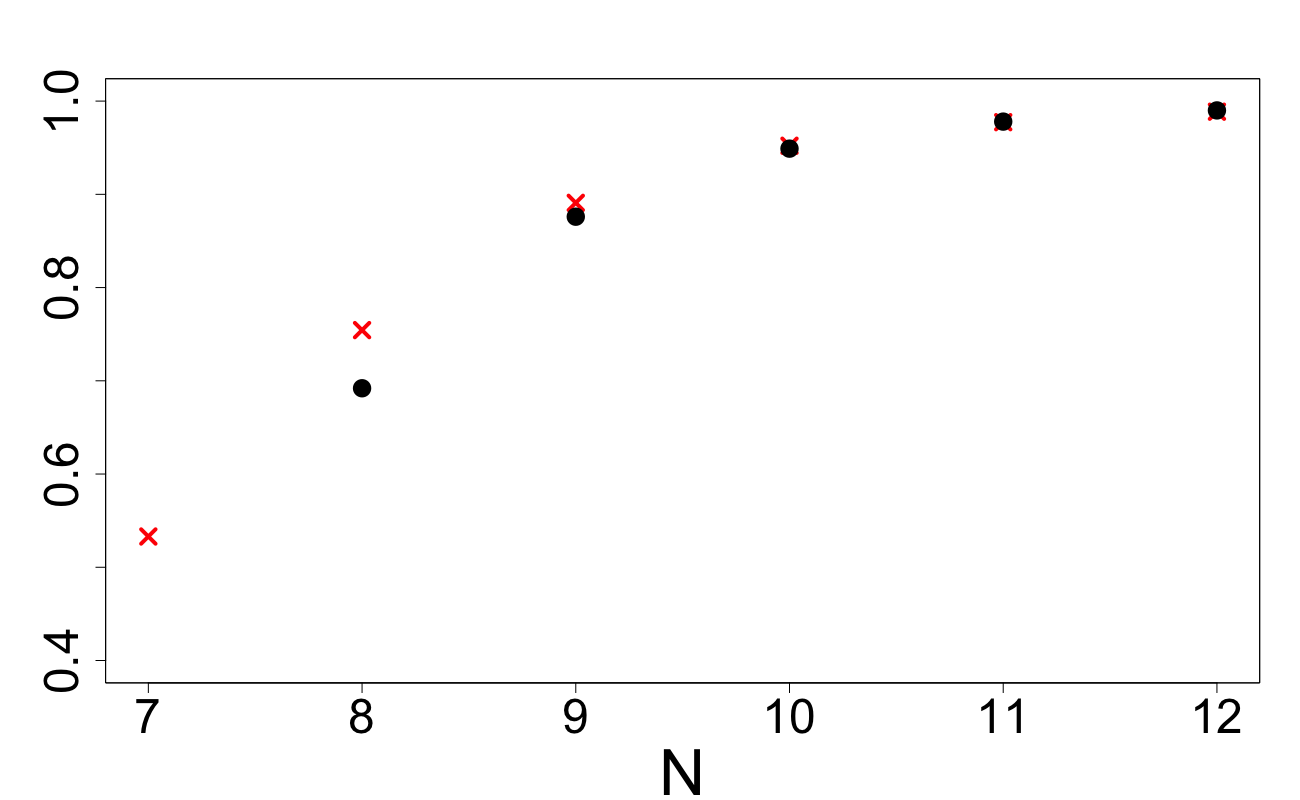
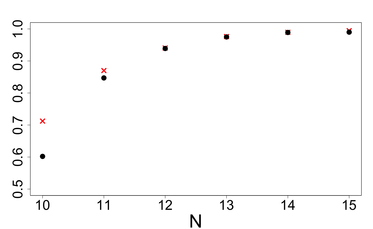
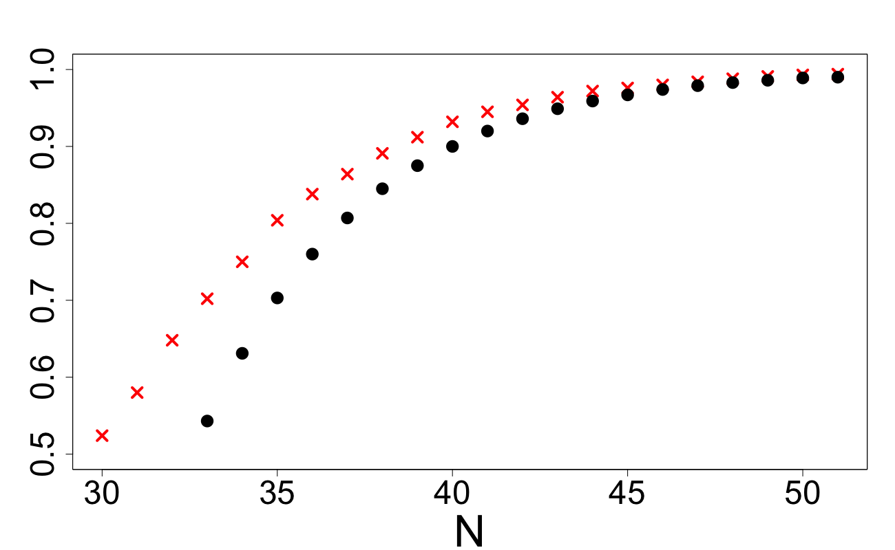
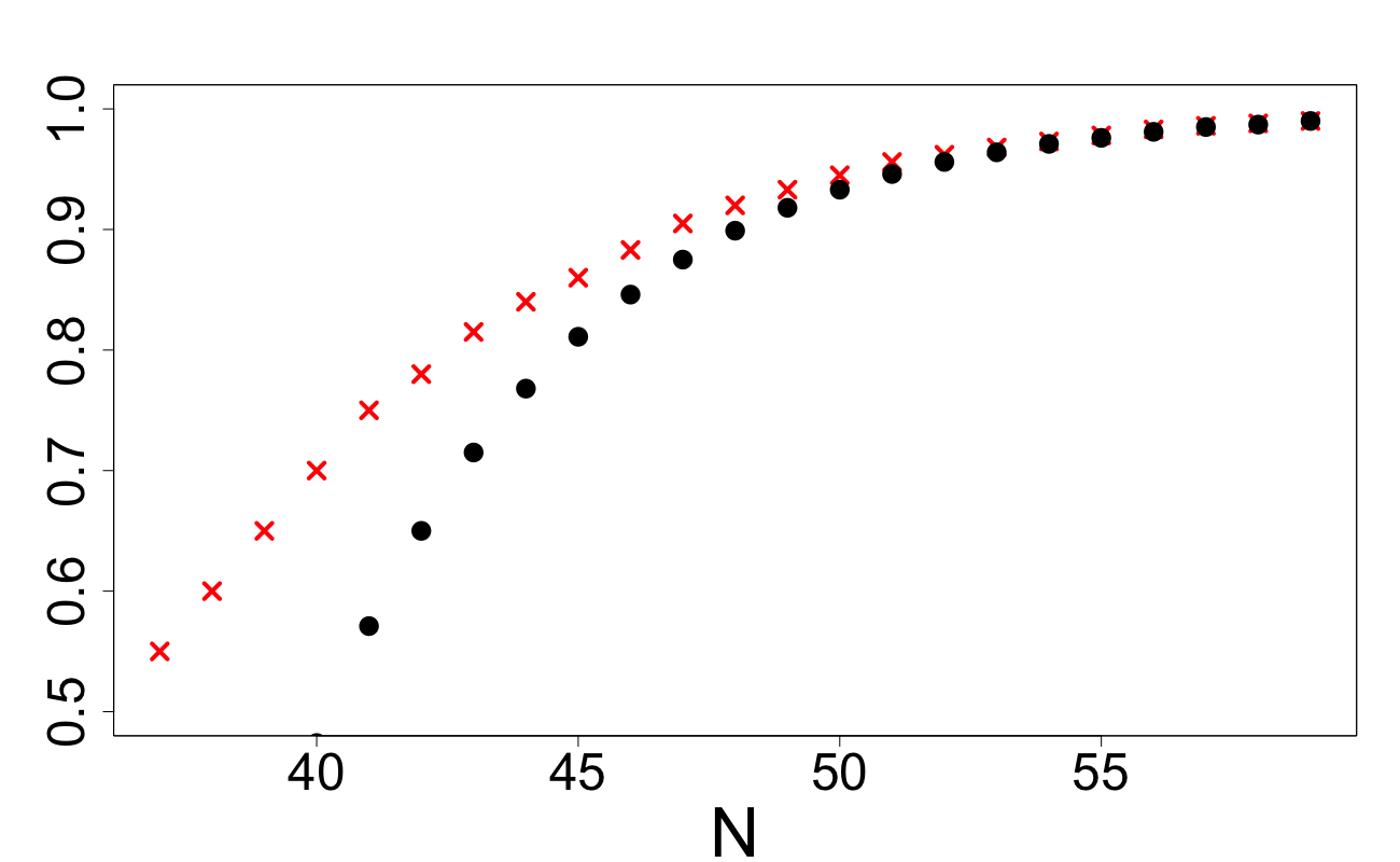
In Figures 3–3, using red crosses we depict the probability ${{\rm Pr}_{{\mathbb{Q}},{\mathbb{R}}}\{T\textrm{ is separated by }{D}_{N}\}}$ as a function of $N$. These values have been obtained via Monte Carlo simulations with $50,000$ repetitions. With the black dots we plot the value of $1-\gamma$ as a function of $N_{\gamma}$. For these figures, we have set ${\cal T}={\cal P}_{n}^{3}$ and chosen $s=n/2$ based on the asymptotic considerations discussed in the beginning of Section 5.4.

In Tables 1–2, for a given value of $1-\gamma^{*}$ we tabulate the value of $1-\gamma$ for the additive group testing model, where ${\cal T}={\cal P}_{n}^{3}$, ${\cal D}={\cal P}_{n}^{s}$ and ${\mathbb{Q}}$ and ${\mathbb{R}}$ are uniform on ${\cal T}$ and ${\cal D}$ respectively. The values have been obtained via Monte Carlo simulations. When considering the inverse problem discussed in (2.3), we also include the explicit upper bounds $N_{\gamma}$ and the value of $N_{\gamma^{*}}$ obtained via Monte Carlo for different values of $n,s$ and $\gamma^{*}$. In all Monte Carlo simulations, we have used $50,000$ repetitions. Tables 1–2 and Figures 3–3 demonstrate that when $\gamma^{*}$ is small, the union bound used in the proof of Theorem 2.1 appears very sharp since the values of $1-\gamma$ and $1-\gamma^{*}$ almost coincide.

Figure 2: Additive model; $n=20,s=10$.

Figure 3: Additive model; $n=50,s=25$.

	$n=20$			$n=50$			$n=100$			$n=150$
$\lambda$	$N_{\gamma^{*}}$	$N_{\gamma}$	$1-\gamma$	$N_{\gamma^{*}}$	$N_{\gamma}$	$1-\gamma$	$N_{\gamma^{*}}$	$N_{\gamma}$	$1-\gamma$	$N_{\gamma^{*}}$	$N_{\gamma}$	$1-\gamma$
0.10	31	34	0.96	38	40	0.96	42	44	0.97	42	46	0.96
0.20	16	17	0.96	19	21	0.97	21	23	0.96	23	24	0.96
0.30	11	12	0.97	14	15	0.97	14	16	0.97	17	18	0.97
0.40	9	11	0.98	11	13	0.98	13	15	0.98	14	16	0.98
0.50	8	11	0.98	11	13	0.98	12	14	0.98	13	15	0.98

Table 1: Additive model with $\gamma^{*}=0.05$, $d=3$ $s=\lceil\lambda n\rceil$, various $n$ and $\lambda$.

	$n=20$			$n=50$			$n=100$			$n=150$
$\lambda$	$N_{\gamma^{*}}$	$N_{\gamma}$	$1-\gamma$	$N_{\gamma^{*}}$	$N_{\gamma}$	$1-\gamma$	$N_{\gamma^{*}}$	$N_{\gamma}$	$1-\gamma$	$N_{\gamma^{*}}$	$N_{\gamma}$	$1-\gamma$
0.10	28	30	0.92	34	36	0.93	38	40	0.93	41	43	0.94
0.20	15	16	0.93	17	19	0.93	20	21	0.93	21	22	0.93
0.30	9	11	0.94	12	14	0.94	14	15	0.95	15	17	0.95
0.40	8	10	0.95	10	12	0.95	12	14	0.95	13	15	0.96
0.50	8	10	0.96	10	12	0.97	12	14	0.96	12	14	0.97

Table 2: Additive model with $\gamma^{*}=0.1$, $d=3$ $s=\lceil\lambda n\rceil$, various $n$ and $\lambda$.

3.4 Extension for ${\cal D}\neq{\cal P}_{n}^{s}$

In this section we demonstrate how the key results of the Sections 3.1 and 3.2 can be easily modified for the case when ${\cal D}=\cup_{s}{\cal P}_{n}^{s}$, where the union is taken over any subset of $\{0,1,\ldots,n\}$, and for a distribution ${\mathbb{R}}$ that is not necessarily uniform on ${\cal D}$.

Let ${\cal D}={\cal P}_{n}^{\leq n}$, ${\mathbb{S}}$ be a probability distribution on $\{0,1,\ldots,n\}$ and $\zeta$ be a ${\mathbb{S}}$-distributed random variable on $\{0,1,\ldots,n\}$. The distribution ${\mathbb{R}}$ depends on ${\mathbb{S}}$ in the following way: for a ${\mathbb{R}}$-distributed random test $X\in{\cal D}$ we have

$$\mbox{Pr}_{{\mathbb{R}}}\{|X|={s}\}=\mbox{Pr}_{\mathbb{S}}\{\zeta={s}\},\,\,\ \mbox{Pr}_{{\mathbb{R}}}\{X=x\,|\,|X|={s}\}=1/{{n\choose s}}\,\,\,\,\mbox{$\forall x\in{\cal P}_{n}^{s}$, else 0}\,.$$ (3.6)

These two requirements mean that for all $s\in\{0,1,\ldots,n\}$ and $\textsf{X}\in{\cal P}_{n}^{s}$ we have

$$\mbox{Pr}_{{\mathbb{R}}}\{X=\textsf{X}\}={\mbox{Pr}_{\mathbb{S}}\{\zeta=s\}}/{{n\choose s}}\,.$$

Note that in the case of Bernoulli design, when each item is included into a group of items with probability $p$, ${\mathbb{S}}$ is Bin($n,p$), the Binomial distribution with parameters $n$ and $p$.

For a general test function $f(X,T)$ we introduce the probability

$$p_{ijs}=\mbox{Pr}\{f(X,T_{i})=f(X,T_{j})\,|\,|X|=s\}.$$

By conditioning on $s$, we obtain $p_{ij}=\sum_{s=0}^{n}p_{ijs}\mbox{Pr}_{\mathbb{S}}\{\zeta={s}\}.$ In view of the conditional uniformity of ${\mathbb{R}}$, which is the second condition in (3.6), the probabilities $p_{ijs}$ can be written as

$$p_{ijs}={k_{ijs}}/{|{\cal P}_{n}^{s}|}={k_{ijs}}/{{{n\choose s}}}$$

where $k_{ijs}=k(T_{i},T_{j},s)\,$ is the number of $X\in{\cal P}_{n}^{s}$ such that $f(X,T_{i})\,=\,f(X,T_{j});\;$ that is,

$$k_{ijs}=\left|\{X\in{{\cal P}_{n}^{s}}:\;f(X,T_{i})=f(X,T_{j})\}\right|\;\;\;\;\;\mbox{\rm for $\;\;T_{i},T_{j}\in{{\cal T}}$}\,.$$

From this, we obtain

$$p_{ij}=\sum_{s=0}^{n}{k_{ijs}}\mbox{Pr}_{\mathbb{S}}\{\zeta={s}\}/{{{n\choose s}}}\,.$$

Set

$$q_{{\cal D},n,l,m,p;\,{\mathbb{S}}}=\sum_{s=0}^{n}\frac{K({\cal P}_{n}^{s},n,l^{\prime},m^{\prime},p)}{{n\choose s}}\mbox{Pr}_{\mathbb{S}}\{\zeta={s}\}\;\;{\rm with}\;\;l^{\prime}=\max(l,m),m^{\prime}=\min(l,m)\,.$$

Then all results of the previous sections established for the case ${\cal D}={\cal P}_{n}^{s}$ can be can be extended for the group testing problems with ${\cal D}=\cup_{s}{\cal P}_{n}^{s}$ by replacing $q_{{\cal D},n,l,m,p}$ of (3.2) with $q_{{\cal D},n,l,m,p;\,{\mathbb{S}}}$.

4 Group testing for the binary model

4.1 A general result and its specialization to particular cases

In the binary group testing, we have ${h}=1$ in (1.1) and thus the test function is

$$f(X,T)=f_{1}(X,T)=\left\{\begin{array}[]{ll}0&\;\mbox{ if }\;|X\cap T|=\emptyset,\\ 1&\mbox{ otherwise.}\end{array}\right.$$ (4.3)

Theorem 4.1

Let the test function be (4.3), $0\leq p\leq m\leq l\leq n$, $p<l$, ${\cal D}={\cal P}_{n}^{s}$ and $(T_{i},T_{j})\in{\cal T}(n,l,m,p)$. Then the value of the Rényi coefficient $k_{ij}$ does not depend on the choice of the pair $(T_{i},T_{j})\in{\cal T}(n,l,m,p)$ and equals $k_{ij}=K({\cal P}_{n}^{s},n,l,m,p),$ where

$$K({\cal P}_{n}^{s},n,l,m,p)={{n}\choose{s}}-{{n-l}\choose{s}}-{{n-m}\choose{s}}+2{{n-l-m+p}\choose{s}}\,.$$ (4.4)

The proof of Theorem 4.1 can be obtained from Zhigljavsky (2003) and is included in Appendix A for completeness.

Corollary 3

Let the test function be (4.3) and set $n\geq 2$, $1\leq d<n$, $1\leq s<n$ and ${\cal D}={\cal P}_{n}^{s}$. For a fixed $N\geq 1$, let ${D}_{N}=\{X_{1},\ldots,X_{N}\}$ be a random $N$-point design with each $X_{i}\in{D}_{N}$ chosen independently and ${\mathbb{R}}$-distributed, where ${\mathbb{R}}$ is the uniform distribution on ${\cal D}$. We consider the following cases for ${\cal T}={\cal P}_{n}^{d}$ and ${\mathbb{Q}}$:

1. Let ${\cal T}={\cal P}_{n}^{d}$ and ${\mathbb{Q}}$ be the uniform distribution on ${\cal T}$. For a fixed $N\geq 1$, let ${D}_{N}=\{X_{1},\ldots,X_{N}\}$ be a random $N$-point design with each $X_{i}\in{D}_{N}$ independent and ${\mathbb{R}}$-distributed. Then $\gamma^{*}({\mathbb{Q}},{\mathbb{R}},N)$ can be obtained from (3.4) with

   $${K({\cal P}_{n}^{s},n,d,d,p)}={{n\choose s}}-2{{{n-d}\choose{s}}+2{{n-2d+p}\choose{s}}}\,.$$

2. Let ${\cal T}={\cal P}_{n}^{\leq d}$ and ${\mathbb{Q}}$ be a distribution satisfying (2.17). Then $\gamma^{*}({\mathbb{Q}},{\mathbb{R}},N)$ can be obtained from (3.3) with

   $$q_{{\cal D},n,{b},m,p}=1{-}\left[{\left({n{-}{b}}\atop{s}\right)+\left({n{-}m}\atop{s}\right){-}2\left({n{-}{b}{-}m{+}p}\atop{s}\right)}\right]\big{/}{\left({n}\atop{s}\right)}\,.$$ (4.5)

3. Let ${\cal T}={\cal P}_{n}^{\leq n}$, ${\mathbb{Q}}$ be a distribution satisfying (2.17) and suppose ${\mathbb{B}}$ is the $Bin(n,q)$ distribution on $\{0,1,\ldots n\}$ for some $q>0$. Then application of Theorem 3.2 provides

   $$\gamma^{*}({\mathbb{Q}},{\mathbb{R}},N)=\sum_{{b}=0}^{n}{n\choose{b}}q^{b}(1-q)^{n-{b}}\min\left\{1,\frac{1}{{{n}\choose{{b}}}}\sum_{m=0}^{n}\,\sum_{p=0}^{\min\{{b},m\}}\!{\textstyle{{n}\choose{p\;m-p\;{b}-p\;n-{b}-m+p}}}q^{N}_{{\cal D},n,{b},m,p}\right\}$$

   with $q_{{\cal D},n,{b},m,p}$ obtained from (4.5).

In Table 3, using the results of part one of Corollary 3 we consider the inverse problem discussed in (2.3) and tabulate the value of $N_{\gamma}$ supposing ${\cal T}={\cal P}_{n}^{3}$ for different values of $s$ and $n$. In Table 4, using the results of part three of Corollary 3 we tabulate the value of $N_{\gamma}$ supposing ${\mathbb{B}}$ is the $Bin(n,3/n)$ distribution. In distribution ${\mathbb{B}}$, the probability of success has been set to $3/n$ so that each target $T\in{\cal T}$ will have three elements on average to compare with the results of Table 3. We see the binomial sample problem requires significantly more tests to locate the defective items with high probability than the case of exactly $d$ defectives.

$\lambda$
0.10
0.15
0.20
0.25
0.30

$\gamma=0.01$
$n=20$	$n=50$	$n=100$
47	58	64
37	47	50
33	40	44
32	39	43
34	40	44

$\gamma=0.05$
$n=20$	$n=50$	$n=100$
38	48	54
30	39	42
27	33	37
26	33	36
28	34	38

Table 3: Values of $N_{\gamma}$ for binary model with $d=3$, $s=\lceil\lambda n\rceil$ for various $n$ and $\lambda$.

$\lambda$
0.10
0.15
0.20
0.25
0.30

$\gamma=0.01$
$n=20$	$n=50$	$n=100$
90	119	142
84	117	184
105	187	410
166	283	731
316	547	1334

$\gamma=0.05$
$n=20$	$n=50$	$n=100$
71	95	113
63	91	154
70	129	242
101	186	380
170	330	604

Table 4: Values of $N_{\gamma}$ for binary model with ${\mathbb{B}}$ the $Bin(n,3/n)$ distribution, $s=\lceil\lambda n\rceil$ for various $n$ and $\lambda$.

The results below will address the scenario of Bernoulli designs. In the following corollaries we set ${\cal D}={\cal P}_{n}^{\leq n}$ and ${\mathbb{S}}$ is the $Bin(n,\kappa)$ distribution for some $0<\kappa<1$. The discussion of Section 3.4 results in the following.

Corollary 4

Let the test function be (4.3) and set $n\geq 2$, $1\leq d<n$, $1\leq s<n$. Let ${\cal D}={\cal P}_{n}^{\leq n}$, ${\mathbb{R}}$ be a distribution satisfying the constraints (3.6) and suppose ${\mathbb{S}}$ is the $Bin(n,\kappa)$ distribution on $\{0,1,\ldots n\}$. Let ${D}_{N}=\{X_{1},\ldots,X_{N}\}$ be a random design with each $X_{i}\in{D}_{N}$ chosen independently and ${\mathbb{R}}$-distributed. We consider the following cases for ${\cal T}={\cal P}_{n}^{d}$ and ${\mathbb{Q}}$:

1. Let ${\cal T}={\cal P}_{n}^{d}$ and ${\mathbb{Q}}$ be the uniform distribution on ${\cal T}$. Then $\gamma^{*}({\mathbb{Q}},{\mathbb{R}},N)$ can be obtained from (3.4) by replacing ${K({\cal P}_{n}^{s},n,d,d,p)}/{{n\choose s}}$ with

   $$\sum_{s=0}^{n}\frac{K({\cal P}_{n}^{s},n,d,m,p)}{{n\choose s}}{\rm Pr}_{\mathbb{S}}\{S={s}\}=1-2\sum\limits_{s=0}^{n}\left({n-d\choose s}-{n-2d+p\choose s}\right)\kappa^{s}(1-\kappa)^{n-s}\,.$$

2. Let ${\cal T}={\cal P}_{n}^{\leq n}$, ${\mathbb{Q}}$ be a distribution satisfying the constraint (2.17) and suppose ${\mathbb{B}}$ is the $Bin(n,q)$ distribution on $\{0,1,\ldots n\}$. Then from (3.3) we obtain

   $$\!\!\gamma^{*}({\mathbb{Q}},{\mathbb{R}},N)\!=\!\sum_{{b}=0}^{n}{n\choose{b}}q^{b}(1\!-\!q)^{n-{b}}\min\left\{1,\frac{1}{{{n}\choose{{b}}}}\sum_{m=0}^{n}\,\sum_{p=0}^{\min\{{b},m\}}\!{\textstyle{{n}\choose{p\;m-p\;{b}-p\;n-{b}-m+p}}}q^{N}_{{\cal D},n,{b},m,p,\kappa}\right\},\;\;\;\;$$

   where

   $$q_{{\cal D},n,{b},m,p,\kappa}=1{-}\sum\limits_{s=0}^{n}\left({{{n{-}{b}}\choose{s}}+{{n{-}m}\choose{s}}{-}2{{n{-}{b}{-}m{+}p}\choose{s}}}\right)\kappa^{s}(1-\kappa)^{n-s}\,.$$

In Table 5, using the results of part one of Corollary 3 we tabulate the value of $N_{\gamma}$ supposing ${\cal T}={\cal P}_{n}^{d}$ with $d=3$ for different values of $s$ and $n$. This table considers more choices for $s$ when compared to Table 3. In Table 6, we tabulate the value of $N_{\gamma}$ obtained via part one of Corollary 4 supposing ${\mathbb{S}}$ is the $Bin(n,\lceil\lambda n\rceil/n)$ distribution. The probability parameter has been set to $\lceil\lambda n\rceil/n$ such that each $X_{i}$ in ${D}_{N}=\{X_{1},\ldots,X_{N}\}$ will have $\lceil\lambda n\rceil$ elements on average to compare with the results of Table 5. The results of these tables indicate it is preferable to have a design with constant-row-weight rather than including each item in a test with some fixed probability (at least for choices of $s$ of interest).

$\lambda$
0.05
0.10
0.15
0.20
0.25
0.30
0.35
0.40
0.45
0.50

$\gamma=0.01$
$n=10$	$n=20$	$n=50$	$n=100$
35	82	86	112
35	47	58	64
25	33	43	48
25	33	40	44
27	32	39	43
27	34	40	44
37	43	45	48
37	43	50	54
62	52	62	64
62	66	73	79

$\gamma=0.05$
$n=10$	$n=20$	$n=50$	$n=100$
28	66	72	94
28	38	48	54
20	27	36	41
20	27	33	37
22	26	33	36
22	28	34	38
29	35	38	41
29	35	42	46
51	43	52	55
51	55	63	69

Table 5: Values of $N_{\gamma}$ for binary model with $d=3$, $s=\lceil\lambda n\rceil$ for various $n$ and $\lambda$.

$\lambda$
0.05
0.10
0.15
0.20
0.25
0.30
0.35
0.40
0.45
0.50

$\gamma=0.01$
$n=10$	$n=20$	$n=50$	$n=100$
49	96	92	115
49	55	61	66
34	38	46	49
34	38	42	45
34	37	41	44
34	38	42	45
41	46	46	49
41	46	51	55
58	53	62	64
58	65	73	79

$\gamma=0.05$
$n=10$	$n=20$	$n=50$	$n=100$
39	78	76	97
39	44	51	56
27	31	38	42
27	31	35	38
27	30	34	37
27	31	35	38
33	37	39	41
33	37	43	47
47	44	52	55
47	54	62	69

Table 6: Values of $N_{\gamma}$ for binary model with ${\mathbb{S}}$ the $Bin(n,\lceil\lambda n\rceil/n)$ distribution for various $n$ and $\lambda$.

4.2 Simulation study

In Tables 7–9, for a given value of $1-\gamma^{*}$ we tabulate the value of $1-\gamma$ for the binary group testing model, where ${\cal T}={\cal P}_{n}^{d}$, ${\cal D}={\cal P}_{n}^{s}$ and ${\mathbb{Q}}$ and ${\mathbb{R}}$ are uniform on ${\cal T}$ and ${\cal D}$ respectively. Similarly to Tables 1–2, we also include the explicit upper bounds $N_{\gamma}$ and the value of $N_{\gamma^{*}}$ obtained via Monte Carlo methods with $50,000$ trials for different values of $n,s$ and $\gamma^{*}$. We see once again, that for small values of $\gamma^{*}$, the union bound used in Theorem 2.1 appears very sharp.

In Figures 5–7, using red crosses we depict the probability ${{\rm Pr}_{{\mathbb{Q}},{\mathbb{R}}}\{T\textrm{ is separated by }{D}_{N}\}}$ as a function of $N$ obtained with $50,000$ Monte Carlo simulations. With the black dots we plot the value of $1-\gamma$ as a function of $N_{\gamma}$. For these figures, we have chosen $s=\lfloor(1-2^{-1/d})n\rfloor$ based on the asymptotic considerations discussed in the beginning of Section 5.4.

	$n=20$			$n=50$			$n=100$			$n=200$
$\lambda$	$N_{\gamma^{*}}$	$N_{\gamma}$	$1-\gamma$	$N_{\gamma^{*}}$	$N_{\gamma}$	$1-\gamma$	$N_{\gamma^{*}}$	$N_{\gamma}$	$1-\gamma$	$N_{\gamma^{*}}$	$N_{\gamma}$	$1-\gamma$
0.10	36	38	0.96	44	48	0.96	49	54	0.96	55	59	0.97
0.20	25	27	0.96	30	33	0.96	33	37	0.96	38	41	0.96
0.30	29	31	0.96	33	35	0.96	35	38	0.97	39	41	0.96
0.40	33	35	0.96	37	42	0.97	42	46	0.97	47	51	0.96
0.50	52	55	0.97	57	63	0.97	62	69	0.98	68	76	0.97

Table 7: Binary model with $\gamma^{*}=0.05$, $d=3$ $s=\lceil\lambda n\rceil$, various $n$ and $\lambda$.

	$n=20$			$n=50$			$n=100$			$n=200$
$\lambda$	$N_{\gamma^{*}}$	$N_{\gamma}$	$1-\gamma$	$N_{\gamma^{*}}$	$N_{\gamma}$	$1-\gamma$	$N_{\gamma^{*}}$	$N_{\gamma}$	$1-\gamma$	$N_{\gamma^{*}}$	$N_{\gamma}$	$1-\gamma$
0.10	32	34	0.92	40	44	0.93	45	50	0.93	51	55	0.94
0.20	22	24	0.92	28	31	0.93	32	34	0.92	36	38	0.93
0.30	26	28	0.93	30	32	0.93	33	35	0.93	36	38	0.93
0.40	29	32	0.93	35	39	0.94	39	43	0.94	44	47	0.94
0.50	46	51	0.95	52	59	0.96	58	65	0.96	64	72	0.95

Table 8: Binary model with $\gamma^{*}=0.1$, $d=3$ $s=\lceil\lambda n\rceil$, various $n$ and $\lambda$.

	$n=20$			$n=50$			$n=100$			$n=200$
$\lambda$	$N_{\gamma^{*}}$	$N_{\gamma}$	$1-\gamma$	$N_{\gamma^{*}}$	$N_{\gamma}$	$1-\gamma$	$N_{\gamma^{*}}$	$N_{\gamma}$	$1-\gamma$	$N_{\gamma^{*}}$	$N_{\gamma}$	$1-\gamma$
0.10	24	29	0.84	34	39	0.87	38	44	0.87	43	49	0.88
0.20	18	21	0.84	24	27	0.85	26	31	0.86	29	34	0.86
0.30	21	24	0.85	25	28	0.85	27	31	0.85	30	35	0.87
0.40	24	28	0.86	30	35	0.87	34	39	0.88	37	43	0.88
0.50	37	45	0.90	44	53	0.89	50	60	0.92	53	67	0.95

Table 9: Binary model with $\gamma^{*}=0.25$, $d=3$ $s=\lceil\lambda n\rceil$, various $n$ and $\lambda$.

Figure 4: Binary model: $\gamma$ vs $\gamma^{*}$ for $n=100$ and $d=3$.

Figure 5: Binary model: $\gamma$ vs $\gamma^{*}$ for $n=200$ and $d=3$.

Figure 6: Binary model: $\gamma$ vs $\gamma^{*}$ for $n=100$ and $d=4$.

Figure 7: Binary model: $\gamma$ vs $\gamma^{*}$ for $n=200$ and $d=4$.

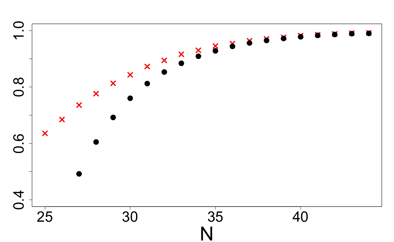
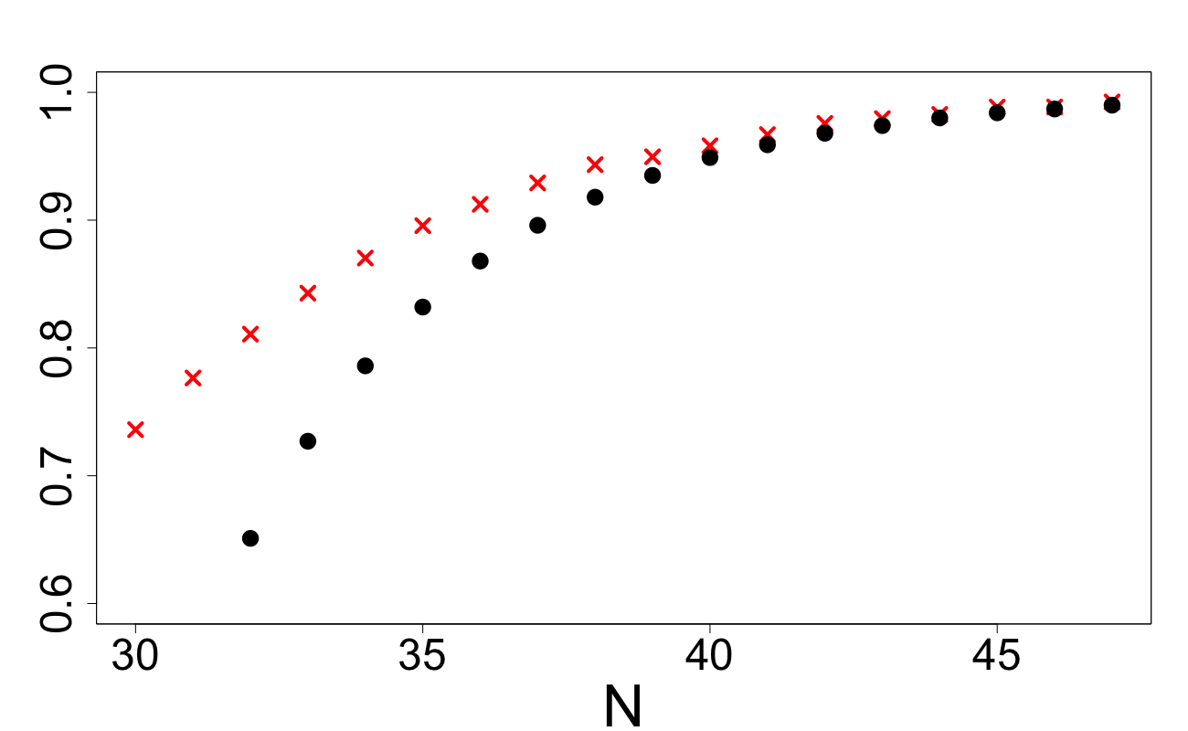
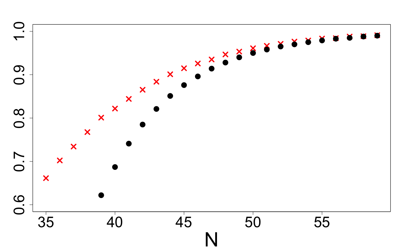
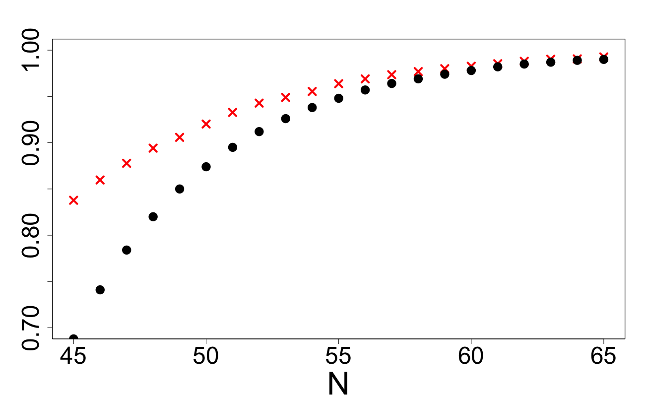
From Tables 7–9 and Figures 5–7 we can draw the following conclusions. For small values of $\gamma$, the value of $\gamma^{*}$ is very close to $\gamma$ (equivalently $N_{\gamma}$ is very close to $N_{\gamma}$). For larger values of $\gamma$, we see that $\gamma^{*}$ is often very conservative with the true $\gamma$ being significantly smaller.

We use the following decoding technique for random designs and improved random designs of Section 4.3. We start with the COMP procedure described in the beginning of Section 4.5 to eliminate uniquely defined non-defective items. Then, in the case where the defective factors are unknown, we perform several additional individual tests to exactly locate the defective items (such tests are very easy to design). In simulation studies we do not need this as the group $T=T_{i}$ consisting of defective items is known and we only need to establish whether there is another group $T^{\prime}=T_{j}$ giving exactly the same test results. In one random test, the probability that the results coincide is $p_{ij}$ defined in (2.5). As follows from formula (4.4), this probability is high only if $|T_{i}\setminus T_{j}|=1$; this is used explicitly in the proof of Theorem 5.1 and noticed in the beginning of Section 5.4. In $N$ tests, such probability becomes $p_{ij}^{N}$ and if $N$ is not very small, $p_{ij}^{N}$ becomes negligible when $|T_{i}\setminus T_{j}|>1$. The probability $\tilde{p}_{ij}$ that both results are 1 are also small when $|T_{i}\setminus T_{j}|>1$. Therefore, for checking whether $T$ is not the unique group of items consistent with all the test results, it is enough to only check item groups $T^{\prime}$ with $|T\setminus T^{\prime}|=1$. The same considerations can be used for the additive and other group testing models.

4.3 Improving on random designs in group testing problems

Any $N$-point design ${D}_{N}=\{X_{1},\ldots,X_{N}\}$ has an equivalent matrix representation as an $N\times n$-matrix ${\cal X}({D}_{N})$ where columns relate to items and rows to test groups. Let $a_{i,j}=1$ if item $a_{j}$ $(j=1,\ldots,n)$ is included into the test group $X_{i}$ $(i=1,\ldots,N)$; otherwise $a_{i,j}=0$. Then the test matrix corresponding to design ${D}_{N}$ is ${\cal X}({D}_{N}):=(a_{i,j})_{i,j=1}^{N,n}\,$. We shall denote the rows of ${\cal X}({D}_{N})$ by ${\cal X}_{i}:=(a_{i,1},\ldots,a_{i,n})$ for $i=1,\ldots,N$. A design is called constant-column-weight design if all columns of ${\cal X}({D}_{N})$ have the same number of ones whereas for a constant-row-weight design all rows of ${\cal X}({D}_{N})$ have the same number of ones. The designs which are both constant-row-weight and constant-column-weight designs are referred to as doubly regular designs, see Section 1.3 in Aldridge et al. (2019). If, for a given design, one of the constancy assumptions is approximately true, we shall use the prefix ‘near-constant’.

In the most important case ${\cal D}={\cal P}_{n}^{s}$, all designs (including random designs and the designs constructed in this section) are automatically constant-row-weight designs. To improve on the separability properties of random designs, we will construct near-constant-column weight designs and hence our designs will be nearly doubly regular designs. Moreover, we will impose restrictions on the Hamming distance between the tests (equivalently the rows of ${\cal X}({D}_{N})$). Summarizing, the designs of this section will have near-constant-column weights, constant-row-weights and have an additional restriction on the Hamming distance between the rows of ${\cal X}({D}_{N})$. Notice that the fact that keeping large Hamming distances between columns of the test matrix ${\cal X}(\cdot)$ tend to improve separability properties of the design has been noted in group testing literature, see e.g. Aldridge et al. (2016). Moreover, the main idea behind the $d$-disjunct designs of Macula Macula (1996) is maximization of the minimal Hamming distance between these columns.

Here we shall describe the algorithm of construction of the nested designs we propose; a formal description as a pseudo-code for the algorithm can be found in Appendix B. We start with a one-element design ${D}_{1}=\{X_{1}\}$, where $X_{1}$ is a random group. At $k$-th step we have a design ${D}_{k-1}=\{X_{1},\ldots,X_{k-1}\}$ and we are looking for a new test group $X_{k}$ to be added to the design ${D}_{k-1}$. To do this, we generate 100 candidate test groups $U_{k}=\{X_{k,1},\ldots,X_{k,100}\}$ with $X_{k,i}\in{\cal P}_{n}^{s}$ according to the following procedure. For 75 of the candidate tests, repeat the following. Check the frequency of occurrence of each item and locate the items with the smallest number of occurrences. If there are greater than $s$ of these items, return a random sample of size $s$. If there are fewer than $s$, say $s^{\prime}$, such lowest-frequency items, return all $s^{\prime}$ items and supplement the remaining $s-s^{\prime}$ items with a random sample from the group containing items that have not appeared the fewest. This describes Algorithm 1 in the Appendix B. To form the remaining 25 candidate tests, we simply sample them randomly from ${\cal D}={\cal P}_{n}^{s}$. The 100 candidate tests chosen in this manner encourage nearly equal column weights of the constructed designs ${D}_{k}$ for all $k$. Of the 100 candidates of the set $U_{k}$, we select a single test group as $X_{k}$ by maximizing the smallest Hamming distance to all previous points in the design ${D}_{k-1}$. Specifically, we locate any test group (or groups) $X^{\prime}\in U_{k}$ such that $\min_{1\leq j\leq k-1}d_{H}(X,X_{j})\to\max_{X\in U_{k}}$. This may result in more than one such $X^{\prime}$. If this occurs, we select the group $X^{\prime}\in U_{k}$ such that $\sum_{i=1}^{N}d_{H}(X^{\prime},X_{i})$ is largest. This whole process is described as Algorithm 2 in Appendix B.

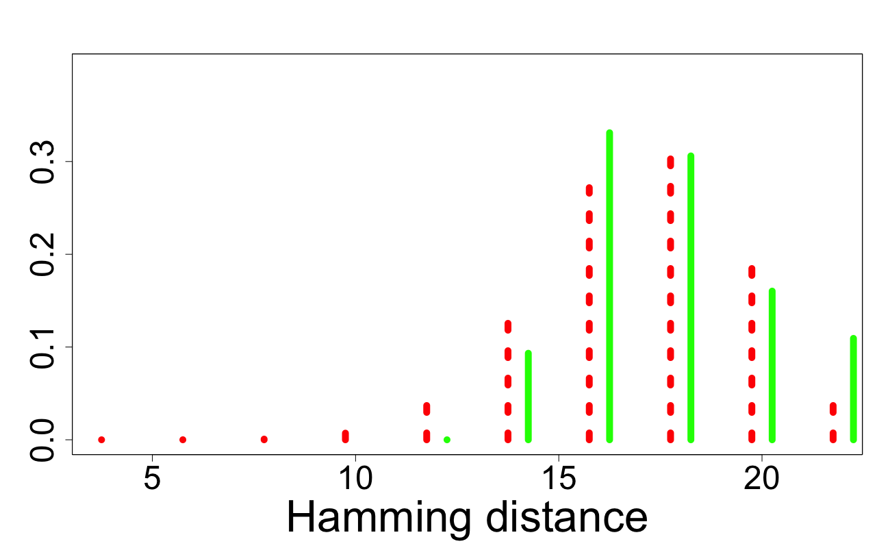
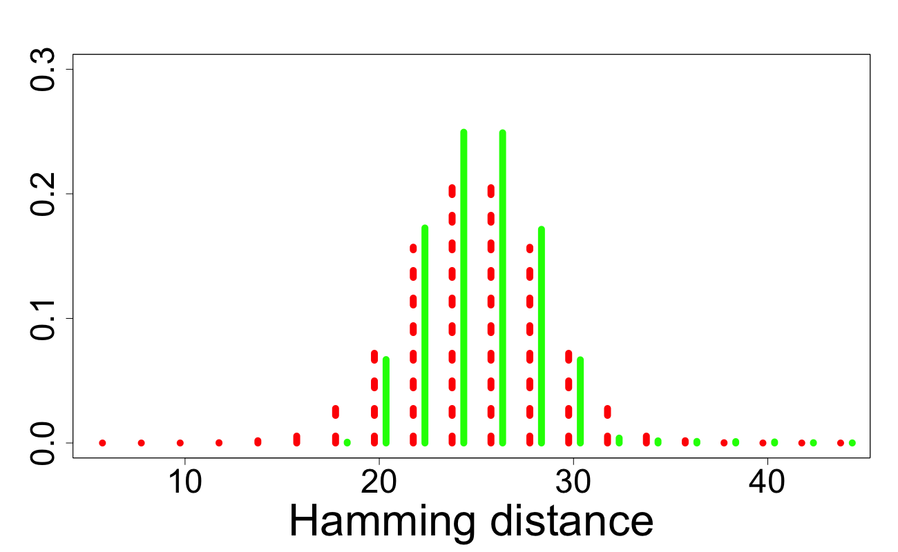
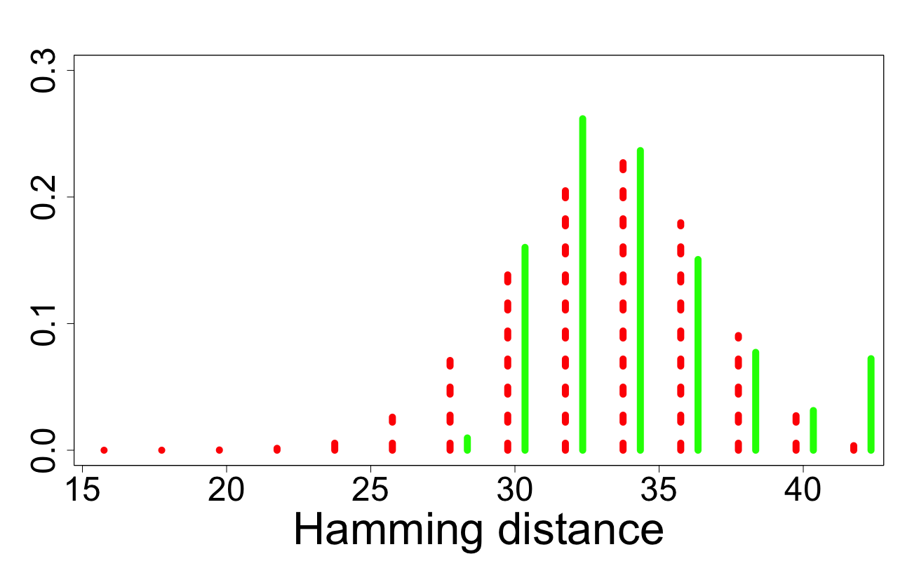
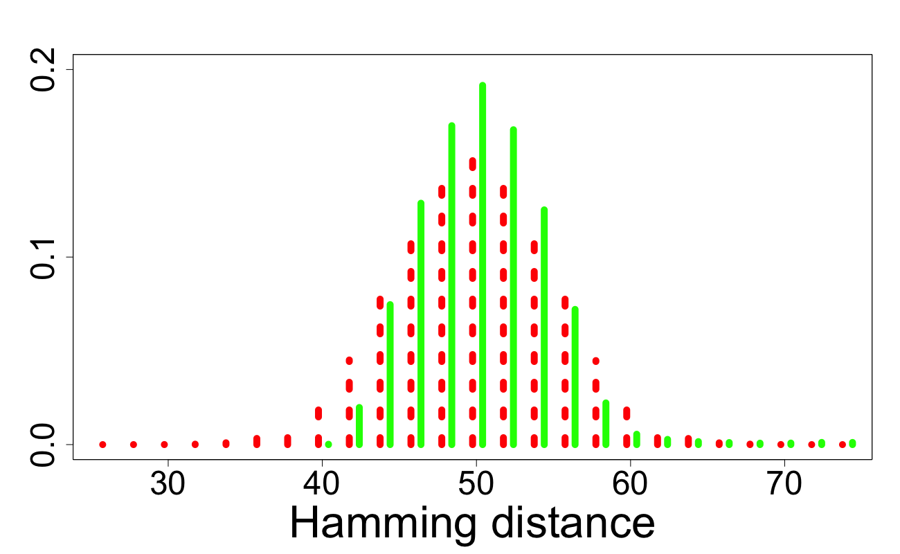
For the random design ${D}_{N}=\{X_{1},\ldots,X_{N}\}$ with each $X_{i}\in{D}_{N}$ chosen independently and uniformly in ${\cal P}_{n}^{s}$, the distribution of the Hamming distance between any two rows of ${\cal X}({D}_{N})$ can be computed. Without loss of generality, we only need to consider the first and second rows of ${\cal X}({D}_{N})$, that is ${\cal X}_{1}$ and ${\cal X}_{2}$. The random variable of interest is $d_{H}({\cal X}_{1},{\cal X}_{2})$. Assume $s\leq n/2$. Then for $x=0,1,\ldots s$ we clearly have

$${\rm Pr}\{d_{H}({\cal X}_{1},{\cal X}_{2})=2x\}={{s\choose s-x}{n-s\choose x}}/{{n\choose s}}\,.$$

In Figures 9–11, we plot the distribution of inter-row distances of ${\cal X}({D}_{N})$ in dotted red and ${\cal X}({D}_{N}^{\prime})$ in solid green, where ${D}_{N}^{\prime}$ is a design obtained by Algorithm 2. The truncation of the lower tail of the distribution in red demonstrates that Algorithm 2 performs very well at preventing small Hamming distances and encouraging large ones.

Figure 8: Distribution of inter-point Hamming distances for random (red) and after the application of Alg. 1 (green); $n=50$ and $s=11$.

Figure 9: Distribution of inter-point Hamming distances for random (red) and after the application of Alg. 1 (green); $n=50$ and $s=25$.

Figure 10: Distribution of inter-point Hamming distances for random (red) and after the application of Alg. 1 (green); $n=100$ and $s=21$.

Figure 11: Distribution of inter-point Hamming distances for random (red) and after the application of Alg. 1 (green); $n=100$ and $s=50$.

4.4 Simulation study for quasi-random designs

In Figures 13–15, we demonstrate the effect Algorithm 2 has on the probability of separation for the binary group testing problem. Using the red crosses we depict the probability ${\rm Pr}_{{\mathbb{Q}},{\mathbb{R}}}\{T\,$ is separated by ${D}_{N}\}$ as a function of $N$. With the black dots we plot the value of $1-\gamma^{*}$ as a function of $N_{\gamma}$. With green plusses we depict the probability of separation when the design ${D}_{N}^{\prime}$ is obtained by Algorithm 2. For these figures we have set $d=3$ and $s=s(n)=\lambda_{d}n$ with $\lambda_{d}$ chosen asymptotically optimally as $\lambda_{d}=1-2^{-1/d}$ (see Section 5.4). From these figures we can see Algorithm 2 significantly increases the probability of separation for the binary testing problem. This is particularly evident for smaller values of $N$.

Figure 12: Binary model with $n=20,s=5$;
random (red) vs improved random (green).

Figure 13: Binary model with $n=50,s=11$;
random (red) vs improved random (green).

Figure 14: Binary model with $n=100,s=21$;
random (red) vs improved random (green).

Figure 15: Binary model with $n=150,s=31$;
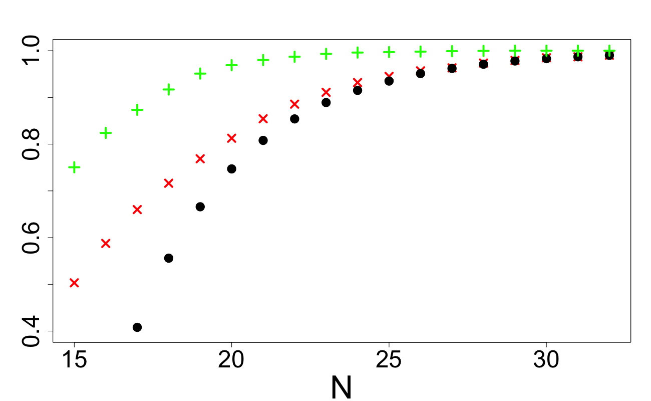
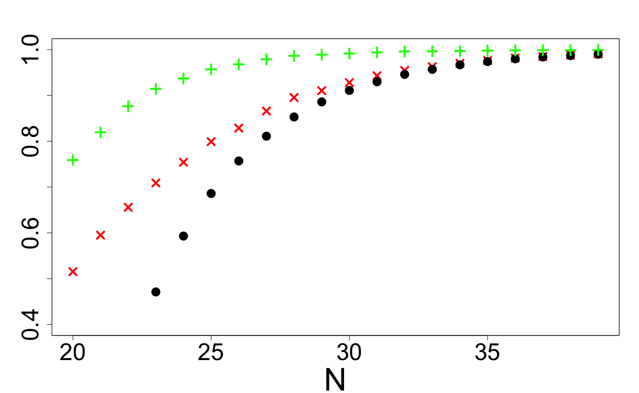
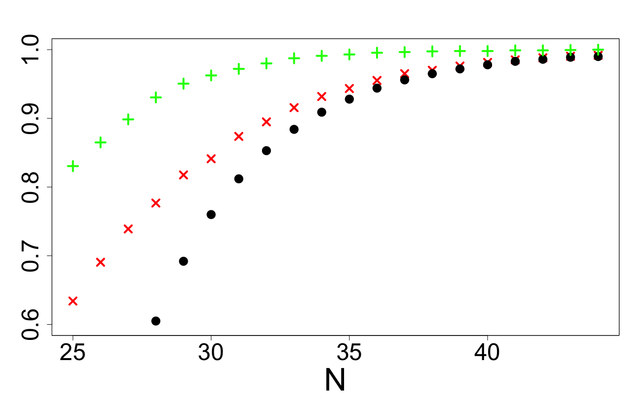
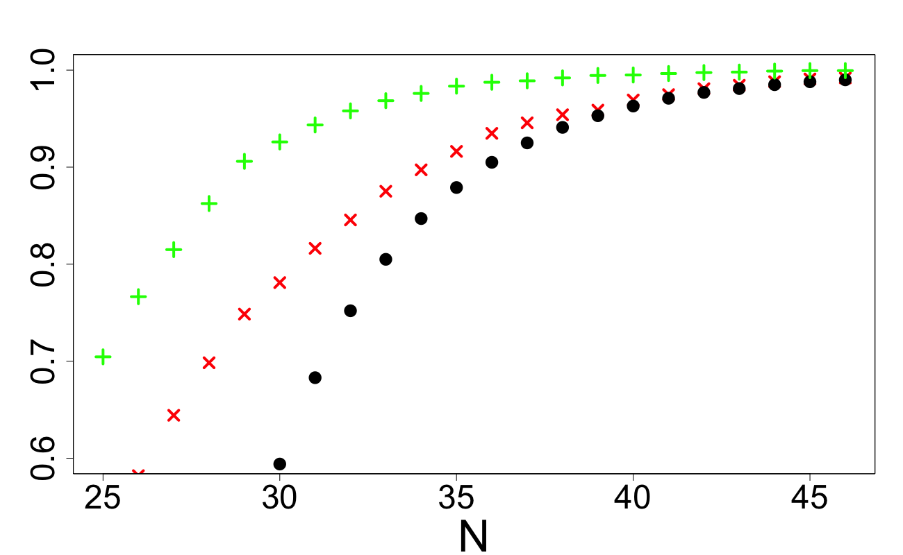
random (red) vs improved random (green).

4.5 Comparison with designs constructed from the disjunct matrices

Given a test matrix ${\cal X}({D}_{N}):=(a_{i,j})_{i,j=1}^{N,n}\,$, let ${\cal S}(a_{j}):=\{i:a_{i,j}=1\}$ denote set of tests in which item $a_{j}$ is included. For a subset ${\cal L}\subseteq{\cal A}$, let ${\cal{S}}({\cal L})=\cup_{a_{j}\in{\cal L}}{\cal S}(a_{j})$. Then a test matrix ${\cal X}={\cal X}({D}_{N})$ is called $d$-disjunct if for any subset ${\cal L}\subseteq{\cal A}$ satisfying $|{\cal L}|=d$ and any $a_{j}\notin{\cal L}$, we never have ${\cal S}(a_{j})\subseteq{\cal{S}}({\cal L})$. A $d$-disjunct matrix can be used to uniquely identify $d$ or less defective items and has the following simple decoding procedure to identify the true defective set: all items in a negative test are identified as non-defective whereas all remaining items are identified as (potentially) defective. This simple procedure is called the combinatorial orthogonal matching pursuit (COMP) algorithm, see (Aldridge et al., 2019, p. 37). Consider the following construction of $d$-disjunct matrices ${\cal X}$.

Let $[m]:=\{1,2,...,m\}$ be a set of integers. Then each of the $n$ columns is labeled by a (distinct) $k$ subset of $[m]$. The numbers $m$ and $k$ must satisfy $n\leq{m\choose k}$. Set ${\cal X}$ to have ${m\choose d}$ rows with each row labeled by a (distinct) $d$-subset of $[m]$, where $d<k<m$; $a_{i,j}$ = 1 if and only if the label of row $i$ is contained in the label of column $j$. It was proved in Macula (1996), that this procedure makes ${\cal X}$ $d$-disjunct. The number of rows in ${\cal X}$, and hence the number of tests performed, is $N={m\choose d}$ which can be very large and can make identification of the defective set expensive. To avoid a large number of tests, it was recommended in Macula (1998) to set $d=2$ regardless of the true $d$; we will call such a matrix 2-disjunct. Whilst the 2-disjunct matrix will no longer guarantee the identification of the defective set if the true $d>2$, it was claimed in Macula (1998), see also D’yachkov et al. (2005), that with high probability the defective set will be identified.

In Tables 10 and 11, we investigate the probability the defective set $T$ is identified when ${\cal T}={\cal P}_{n}^{3}$ and ${\cal T}={\cal P}_{n}^{4}$ for designs constructed by the following three procedures: (a) the design corresponding to the 2-disjunct matrix ${\cal X}$ with the full decoding; (b) the design corresponding to the 2-disjunct matrix ${\cal X}$ with only the COMP procedure used for decoding; (c) ${D}_{N}=\{X_{1},\ldots,X_{N}\}$ with each $X_{i}\in{D}_{N}$ chosen independently and ${\mathbb{R}}$-distributed on ${\cal D}={\cal P}_{n}^{s}$ where $s$ is chosen according to its asymptotically optimal value (see Section 5.4); (d) the design is an improved random design constructed from Algorithm 1. For different values of $n$, when constructing the 2-disjunct matrix ${\cal X}$ we have chosen $m$ and $k$ such that $n\leq{m\choose k}$, $2<k<m$ and $N={m\choose 2}$ is as small as possible. For $n=50,100,200$ and $300$, this results in choosing $m=8$ and $k=3$, $m=9$ and $k=4$, $m=10$ and $k=4$ and $m=11$ and $k=4$ respectively. We have then set the random and improved random designs (constructed from Algorithm 2) (c) and (d) to have the same value of $N$. In these tables, the letter next to $1-\gamma$ corresponds to the procedure used. Within Tables 10 and 11, results have been obtained from Monte Carlo simulations with $100,000$ repetitions.

We can make the following conclusions from the results presented in Tables 10 and 11: (i) random designs are slightly inferior to the designs obtained from 2-disjunct matrices (note, however, that random designs are nested and can be constructed for any $N$), (ii) the COMP decoding procedure alone is insufficient and makes the pair [design, decoding procedure] poor, and (iii) improved random designs constructed by applying Algorithm 1 have much better separability than both random designs and the designs obtained from 2-disjunct matrices.

$n$	$N$	$1-\gamma$ (a)	$1-\gamma$ (b)	$1-\gamma$ (c)	$1-\gamma$ (d)
50	28	0.99	0.82	0.89	0.96
100	36	0.95	0.67	0.95	0.97
200	45	0.98	0.70	0.98	0.98
300	55	0.98	0.77	0.98	0.99

Table 10: Separability comparison for 2-disjunct, random and improved random designs: ${\cal T}={\cal P}_{n}^{3}$.

$n$	$N$	$1-\gamma$ (a)	$1-\gamma$ (b)	$1-\gamma$ (c)	$1-\gamma$ (d)
50	28	0.90	0.51	0.53	0.86
100	36	0.76	0.26	0.70	0.92
200	45	0.86	0.29	0.84	0.96
300	55	0.92	0.38	0.94	0.99

Table 11: Separability comparison for 2-disjunct, random and improved random designs: ${\cal T}={\cal P}_{n}^{4}$.

4.6 Efficiency of the COMP decoding procedure for random designs

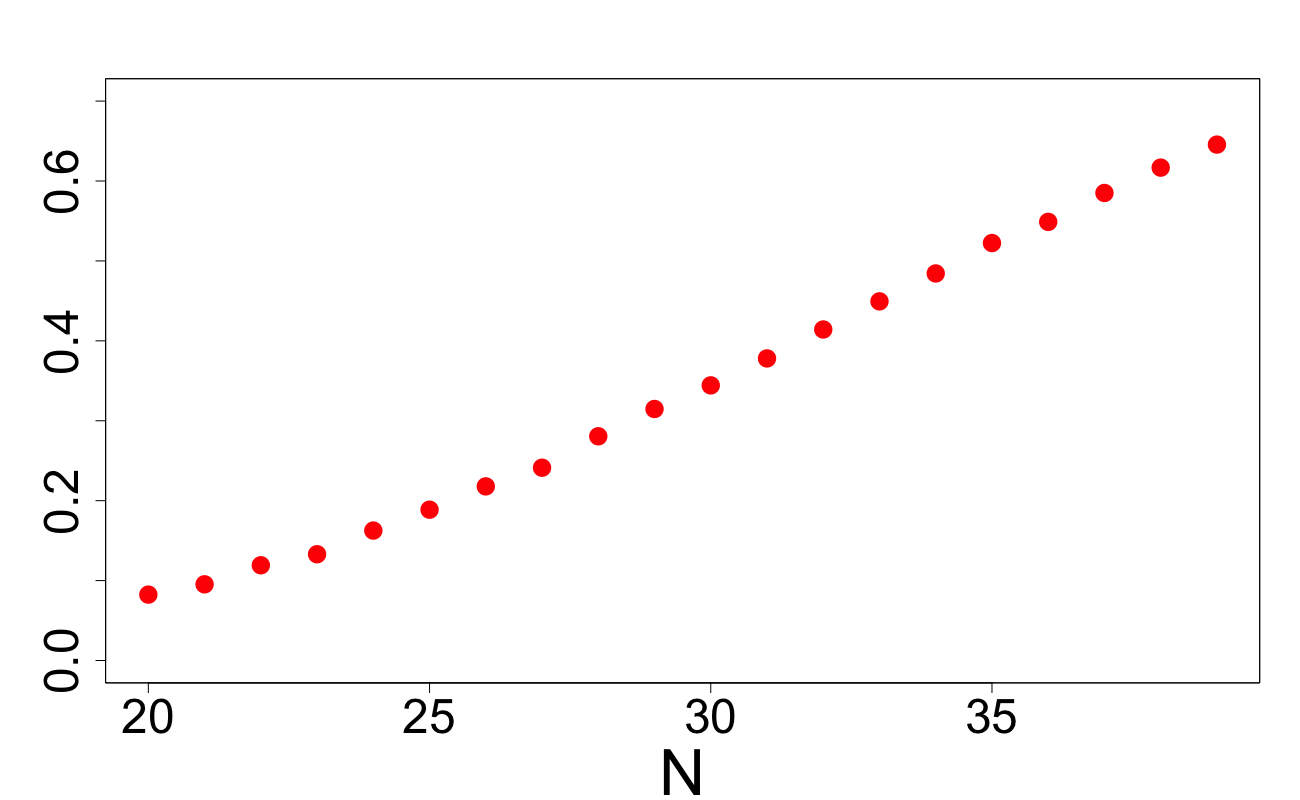
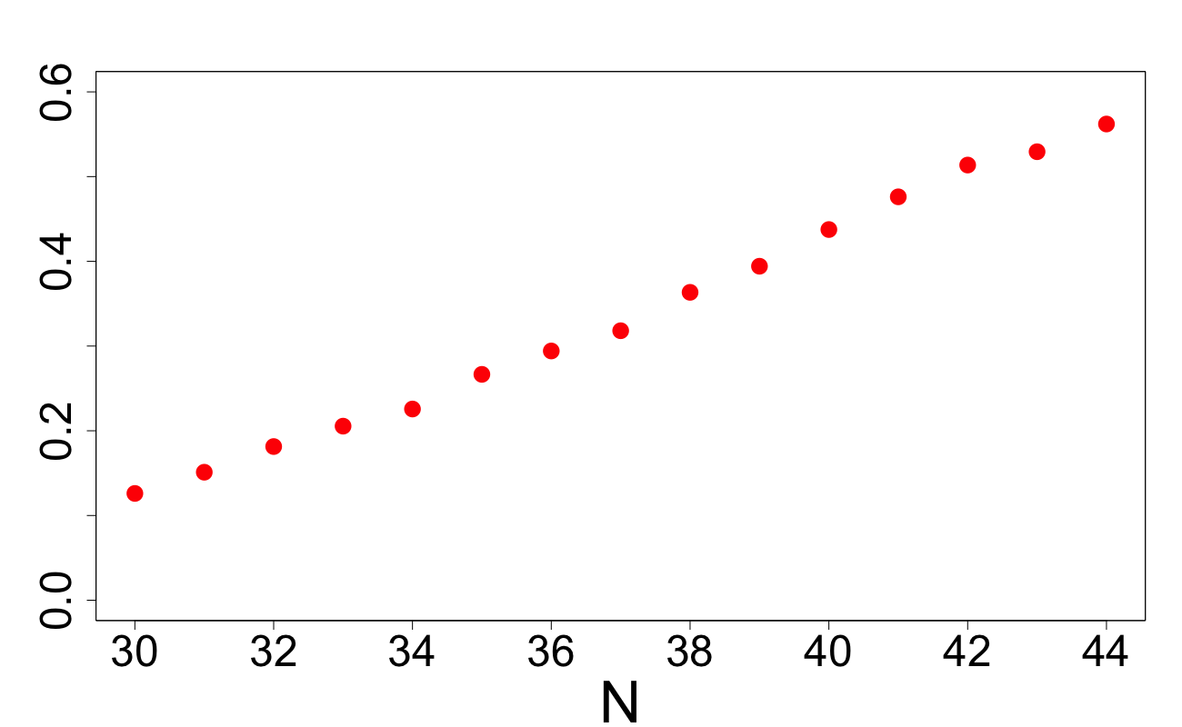
For a disjunct test matrix ${\cal X}$, the COMP decoding procedure described in Section 4.5 is guaranteed to find the defective set and can do so very efficiently (possibly defective items become definitely defective). When the design is not disjunct, say ${D}_{N}$ is constructed randomly, there is no guarantee the COMP procedure will identify the true defective set. Instead, the procedure will provide a set containing the true defective set possibly mixed in with some non-defectives. In (Aldridge et al., 2019, p.37), the set returned by the COMP algorithm is referred to as the largest satisfying set. For situations when the COMP procedure does not return a uniquely defined $T$, further analysis (based on the tests with positive results) must be performed to reduce the number of possible target groups of items $T$ consistent with all available test results. In Figures 17–17, we investigate the efficiency of COMP expressed as the ratio

$${\mbox{Pr}_{{\mathbb{Q}},{\mathbb{R}}}\{\text{COMP decoding returns exactly $T$ for design ${D}_{N}$}\}}/{{{\rm Pr}_{{\mathbb{Q}},{\mathbb{R}}}\{T\textrm{ is separated by }{D}_{N}\}}}\,$$

for the designs ${D}_{N}$ is constructed randomly. The values in these figures have been obtained from Monte Carlo methods with $50,000$ repetitions. From these figures we observe that despite for larger $N$ the COMP procedure has a higher efficiency, this efficiency is still very low. We thus conclude, also taking into account the second conclusion at the end of Section 4.5, for random designs ${D}_{N}$ the COMP procedure alone will not guarantee identification of the target set frequently enough and must be supplemented by further analysis of positive results.

Figure 16: Binary model with $n=50,s=11$.

Figure 17: Binary model with $n=100,s=21$.

4.7 Binary group testing with lies

As discussed in Section 2.3, the results of this paper can be extended to the case where several lies are allowed by introducing the final sum on the right hand side of (2.10). As an example, we shall provide a generalisation of part one of Corollary 3.

Corollary 5

Let the test function be defined by (4.3). Let ${\cal T}={\cal P}_{n}^{d}$ and ${\cal D}={\cal P}_{n}^{s}$, where $n\geq 2$, $1\leq d<n$, $1\leq s<n$ and suppose at most $L$ lies are allowed. Let ${\mathbb{Q}}$ and ${\mathbb{R}}$ be uniform distributions on ${\cal T}$ and ${\cal D}$ respectively. For a fixed $N\geq 1$, let ${D}_{N}=\{X_{1},\ldots,X_{N}\}$ be a random $N$-point design ${D}_{N}$ with each $X_{i}\in{D}_{N}$ chosen independently and ${\mathbb{R}}$-distributed. Then $\gamma^{*}({\mathbb{Q}},{\mathbb{R}},N)$ for the $L$-lie problem can be obtained from (3.4) by replacing

$$\frac{K({\cal P}_{n}^{s},n,d,d,p)}{{n\choose s}}=1-2\cdot\frac{{{n-d}\choose{s}}-{{n-2d+p}\choose{s}}}{{{n}\choose{s}}}\,$$

with

$$\sum_{l=0}^{2L}{{N}\choose{l}}\left(1-2\cdot\frac{{{n-d}\choose{s}}-{{n-2d+p}\choose{s}}}{{{n}\choose{s}}}\right)^{N-l}\left(2\cdot\frac{{{n-d}\choose{s}}-{{n-2d+p}\choose{s}}}{{{n}\choose{s}}}\right)^{l}\,.$$

In Table 12 and Table 13, we document the values of $N^{*}_{\gamma}$ obtained from Corollary 5 for $L=1$ and $L=2$ respectively, for several choices of $s$ and $n$. When comparing these tables with Table 5, we see the significant increase in tests needed when lies are present. In Figures 19–19, using red crosses we depict ${\rm Pr}_{{\mathbb{Q}},{\mathbb{R}}}\{T\textrm{ can be uniquely identified by }{D}_{N}\textrm{ with at most $1$ lies}\}$ as a function of $N$. This has been obtain from Monte Carlo methods with $50,000$ repetitions. With the black dots we plot the value of $1-\gamma^{*}$ as a function of $N_{\gamma}$ obtained via Corollary 5. In these figures we have set $s=n/4$ on the basis of Table 12. We see once again for small values of $\gamma$, the value of $\gamma^{*}$ is very close to $\gamma$ (equivalently $N_{\gamma}$ is very close to $N_{\gamma}$). For larger values of $\gamma$, we see that $\gamma^{*}$ is very conservative.

$\lambda$
0.05
0.10
0.15
0.20
0.25
0.30
0.35
0.40
0.45
0.50

$\gamma=0.01$
$n=10$	$n=20$	$n=50$	$n=100$
56	126	130	166
56	73	87	95
41	52	66	72
41	52	61	66
44	51	59	64
59	53	61	66
59	67	68	71
59	67	75	81
98	81	92	94
98	101	109	115

$\gamma=0.05$
$n=10$	$n=20$	$n=50$	$n=100$
47	108	113	145
47	63	76	83
34	44	58	63
34	44	53	58
37	44	52	56
37	46	53	58
50	58	59	63
50	58	66	71
83	69	81	83
83	87	96	102

Table 12: Values of $N_{\gamma}$ for binary model with $d=3$, $L=1$, $s=\lceil\lambda n\rceil$, various $n$ and $\lambda$.

$\lambda$
0.05
0.10
0.15
0.20
0.25
0.30
0.35
0.40
0.45
0.50

$\gamma=0.01$
$n=10$	$n=20$	$n=50$	$n=100$
73	163	166	210
73	94	111	120
53	67	84	91
53	67	78	84
57	66	76	81
57	69	79	84
77	87	87	91
77	87	96	102
127	104	118	120
127	131	139	146

$\gamma=0.05$
$n=10$	$n=20$	$n=50$	$n=100$
64	143	147	188
64	83	99	108
46	59	75	82
46	59	69	75
50	58	68	73
50	61	70	75
67	77	78	81
67	77	86	92
111	92	105	107
111	115	124	131

Table 13: Values of $N_{\gamma}$ for binary model with $d=3$, $L=2$, $s=\lceil\lambda n\rceil$, various $n$ and $\lambda$.

Figure 18: Lies; binary model with $n=20,L=1,s=5$.

Figure 19: Lies; binary model with $n=50,L=1,s=13$.

5 Asymptotic results

To start this section, let us make a general comment about the asymptotic expansions in group testing. In most of the known expansions (usually based on the use of Bernoulli designs) the authors are interested in the main asymptotic term only. The authors believe that this is not enough if the asymptotic expansions are intended for the use as (even rough) approximations; see, for example, a discussion in Section 5.4 on the asymptotic existence bound in the case of weak recovery in the binary model. All our expansions in the case of very sparse regime (that is, for fixed $d$) are accurate up to the constant term which we have confirmed by numerous numerical studies. As a result, all our sparse-regime asymptotic expansions can be used as rather accurate approximations already for moderate values of $n$ such as $n=1000$. Typically, this is not so if only the leading term in the expansions is kept. The situation in the sparse regime (when $d\to\infty$ but $d/n\to 0$ as $n\to\infty$) is different and depends on the rate of increase of $d$. If $d$ increases as $\log n$ then once again our expansions are rather accurate up to the constant term. However, if $d=n^{\beta}+o(1)$ as $n\to\infty$ with some $0<\beta<1$ then we usually can guarantee only the leading term in the expansions and hence the expansions become pretty useless if one wants to use them for deriving approximations. Moreover, our technique completely fails in the case when $d$ grows like ${\rm const}\!\cdot\!n$ as $n\to\infty$.

5.1 Technical results

The main technical result used for derivation of asymptotic upper bounds in the error-free environment (no lies) for both exact and weak recoveries is Theorem 5.1 in Zhigljavsky (2003), which we formulate below as Theorem 5.1. This theorem is especially useful in the case when ${{\cal D}}={\cal P}_{n}^{s}$ with $s=s(n)=\lambda n+o(1)$ (here $0<\lambda<1$ and $n\to\infty$) and ${{\cal T}}$ is either ${\cal P}_{n}^{d}$ or ${\cal P}_{n}^{\leq d}$ with $d$ fixed (that is, for a very sparse regime). As we show below some results can be extended to a sparse regime when $d\to\infty$ but $d/n\to 0$ as $n\to\infty$. However, unless $d$ tends to infinity very slowly (like $\log n$, for example), we lose the very attractive feature of the expansions, which is the correct constant term.

The authors are not confident that Theorem 5.1 can be applied to the problem of binomial group testing. Also, there are some extra technical difficulties in applying this theorem for Bernoulli designs. At least, we cannot get the constant term $c$ in (5.4) for Bernoulli designs (for these designs, the main term $C\log n$ is the same as for our main case ${{\cal D}}={\cal P}_{n}^{s}$ with $s=\lambda n+o(1)$ and suitable $\lambda$).

Theorem 5.1

Let $I$ be some integer, $c_{i},r_{i},\alpha_{i}$ $(i\!=\!1,\ldots,I)$ be some real numbers, $c_{i}\!>\!0,$ $0\!<\!r_{i}\!<\!1$, at least one of $\alpha_{i}$ be positive, $\{q_{i,n}\}$, $\{r_{i,n}\}$ be families of positive numbers $(i\!=\!1,\dots,I)$ such that $0\!<\!r_{i,n}\!<\!1$ for all $i$ and

$$q_{i,n}=c_{i}n^{\alpha_{i}}(1+o(1)),\quad r_{i,n}=r_{i}+o\left(\frac{1}{\log n}\right)\;\;\;\;{\rm as}\;\;n\rightarrow\infty\,.$$ (5.1)

Define $M(n)$ as the solution (with respect to $M$) of the equation $\sum^{I}_{i=1}q_{i,n}r_{i,n}^{M}\,=1\,$ and set

$$N(n)=\min\,\left\{k=1,2,\ldots\;\mbox{\rm such that }\;\;\sum^{I}_{i=1}q_{i,n}r_{i,n}^{k}\,<1\right\}\,,$$ (5.2)

$$C=\max_{i=1,\ldots,I}\;\frac{\alpha_{i}}{-\log r_{i}}\,.$$ (5.3)

Finally, let $c$ be the solution of the equation $\sum_{j\in{\cal J}}c_{j}r_{j}^{c}\,=1\,,$ where ${\cal J}$ is the subset of the set $\{1,\ldots,I\}$ at which the maximum in (5.3) is attained. Then $N(n)=\lfloor M(n)\rfloor+1$ and

$$M(n)=C\log n+c+o(1)\quad{\rm as}\quad n\rightarrow\infty\,.$$ (5.4)

Note that $C$ and $c$ in (5.4) are constants in the sense that they do not depend on $n$. Extensive numerical results for exact and weak recoveries in the binary, additive and multichannel models show that the resulting asymptotic formula (5.4) (in cases ${{\cal D}}={\cal P}_{n}^{s}$ and ${{\cal T}}={\cal P}_{n}^{d}$ or ${{\cal T}}={\cal P}_{n}^{\leq d}$) is very accurate even for moderate values of $n$. In fact, in all these cases the difference $N(n)-[C\log n+c]$ tends to zero very fast (as $n\to\infty$) as long as $d$ is not too large (here $N(n)$ is the upper bound in any of the existence theorems and is defined in (5.2)). In the sparse regime, when $d\to\infty$ (but $d/n\to 0$), the approximation $N(n)\simeq C\log n+c$ is still accurate but $n$ has to be significantly larger for this approximation to have close to zero accuracy. To distinguish the cases of exact recovery ($\gamma=0$) and weak recovery ($\gamma>0$) we shall write $M_{0}(n)$ for the upper bounds (5.4) in case of exact recovery and $M_{\gamma}(n)$ in case of weak recovery.

As follows from Theorem 3.2 and Corollary 1 of Section 3.1 for weak recovery (similar considerations are true for exact recovery), in cases ${{\cal D}}={\cal P}_{n}^{s}$ and either ${{\cal T}}={\cal P}_{n}^{d}$ or ${{\cal T}}={\cal P}_{n}^{\leq d}$, the existence bounds have the form (5.2). Establishment of the asymptotic relations (5.1), from which everything else follows, is usually a straightforward application of the following two simple asymptotic formulas (see Lemmas 5.1 and 5.2 in Zhigljavsky (2003)).

• Let $n\rightarrow\infty$, $u$ and $w$ be positive integers and $s\!=\!\lambda n\!+\!O(1)$ as $n\rightarrow\infty$ ($0\!<\!\lambda\!<\!1$). Then

  $${{\left({n-w}\atop{s-u}\right)}}\big{/}{{\left({n}\atop{s}\right)}}=\lambda^{u}(1-\lambda)^{w-u}+O\left({1}/{n}\right)\;\;{\rm as}\;\;n\rightarrow\infty\,.$$

• Let $Q(n,l,m,p)$ be as in (2.22), $p$, $m$, $l$ be fixed and $n\rightarrow\infty$. Then

  $$Q(n,l,m,p)=c_{l,m,p}\cdot n^{l+m-p}\left(1+O\left({1}/{n}\right)\right),\quad n\rightarrow\infty\,,$$

  $${\rm with}\;\;\;\; c_{l,m,p}=\left\{\begin{array}[]{ll}{1}/\left[{p!(m\!-\!p)!(l\!-\!p)}\right]&{\rm if}\;\;m\neq l\,,\\ {1}//\left[{2p!((m\!-\!p)!)^{2}}\right]&{\rm if}\;\;m=l\,.\end{array}\right.$$

The set ${\cal J}$ of Theorem 5.1 determines the set (or sets) ${\cal T}(n,l,m,p)$ (see (2.18)) of pairs of target groups $(T,T^{\prime})$ which are most difficult to separate by the random design. Theorem 5.1 establishes that by the time the pairs from these set/s ${\cal T}(n,l,m,p)$ will be separated (in the case of weak recovery, with probability $1-\gamma$), the pairs $(T,T^{\prime})$ from all other sets ${\cal T}(n,l,m,p)$ will be automatically separated with much higher probability which is infinitely close to 1. In most cases, the set ${\cal J}$ defined in Theorem 5.1 contains just one number and hence computation of the constant $c$ in (5.4) is immediate. Even if this is not the case, as in (5.13) below, a very accurate approximation to the exact value of $c$ can be easily found.

5.2 Additive model

For the additive model, the case ${\cal T}={\cal P}_{n}^{\leq d}$ is not very interesting (the same applies to the Binomial testing) as we can make an initial test with all items included into the test group and hence determine the total number of defectives. Therefore, we only consider the case ${\cal D}\!=\!{\cal P}_{n}^{s}$, ${\cal T}\!=\!{\cal P}_{n}^{d}$. Assume $n\rightarrow\infty$, $s=s(n)=\lambda n+O(1)$ when $n\rightarrow\infty$, $0<\gamma<1.$ The optimal value of $\lambda$ is $1/2$, both for weak and exact recovery. For $\lambda=1/2$, ${\cal J}$ consists of the single index corresponding to $l=m=d$ and $p=0$. This gives for exact and weak recovery respectively:

$$M_{0}(n) = (d+1)\log_{2}n\!-\!\log_{2}(d-1)!\!-\!1+o(1)\quad{\rm as}\quad n\rightarrow\infty\,,$$ (5.6)

$$M_{\gamma}(n) = \frac{d\log_{2}n\!-\!\log_{2}(d!\gamma)}{2d\!-\!\log_{2}((2d)!)\!+\!2\log_{2}(d!)}+o(1)\;\;{\rm as}\;n\rightarrow\infty\,.$$ (5.7)

The asymptotic expressions (5.6) and (5.7) have first appeared as (Zhigljavsky and Zabalkanskaya, 1996, Corollary 5.1). Let us make some observations from analyzing formulas (5.6) and (5.7).

First, the denominator $F(d)={2d\!-\!\log_{2}((2d)!)\!+\!2\log_{2}(d!)}$ in (5.7) is monotonically increasing with $d$ from $F(2)=3-\log_{2}3\simeq 1.415$ to $\infty$. This implies that the problem of exact recovery is much more complicated than the problem of weak recovery and ratio of leading coefficients in (5.6) and (5.7) tends to infinity as $d$ increases. This also shows the diminishing role of $\gamma$ in (5.7) and the possibility to allow $\gamma$ to slowly decrease as $d$ increases.

Second, the asymptotic expansion of $F(d)$ at $d=\infty$ is $F(d)=\frac{1}{2}\log_{2}(\pi d)+O\left(1/{d}\right)$ with the respective approximation $F(d)\simeq\frac{1}{2}\log_{2}(\pi d)$ being very accurate for all $d$. Stirling formula also gives $\log_{2}(d!)=d\log_{2}(d/e)+\frac{1}{2}\log_{2}(2\pi d)+O\left(1/{d}\right)$ as $d\to\infty$. This allows us to write the following asymptotic version of (5.7) in the sparse regime with $d=n^{\beta}+O(1)$ and $0<\beta<1$ as

$$\!\!\!M_{\gamma}(n)=\frac{n^{\beta}(1+2(1-\beta)\log n)}{\log(\pi n^{\beta})}\!+O(1)\;\;{\rm as}\;n\!\rightarrow\!\infty\,.$$

The sparse-regime version of (5.6) is very clear and need only the expansion $\log_{2}((d-1)!)=d\log_{2}(d/e)+\frac{1}{2}\log_{2}(2\pi/d)+O\left(1/{d}\right)$ as $d\to\infty$. Thus, for $d=\lfloor n^{\beta}\rfloor$ with $0<\beta<1$ we obtain

$$M_{0}(n)=(\lfloor n^{\beta}\rfloor+1+\beta/2)\log_{2}n\!+O((1)\;\;\;{\rm as}\;n\!\rightarrow\!\infty\,.$$

5.3 Binary model, exact recovery

Consider first the case of exact recovery in the binary model with ${\cal T}={\cal P}_{n}^{d}$, ${\cal D}={\cal P}_{n}^{s}$ and $s=s(n)=\lambda n+O(1)$. From Corollary 5.2 in Zhigljavsky (2003) we obtain the following: the optimal value of $\lambda$ is $\lambda=1/(d+1)$ for which the set ${\cal J}$ of Theorem 5.1 consists of one index corresponding to $l=m=d$ and $p=d-1$; this gives

$$M_{0}(n)=\frac{(d+1)\log_{2}n-\log_{2}(d-1)!-1}{-\log_{2}\left(1-{2d^{d}}/{(d+1)^{d+1}}\right)}\,+o(1)\quad{\rm as}\quad n\rightarrow\infty\,.$$ (5.8)

The numerator in (5.8) coincides with the rhs in (5.6). The denominator in the rhs of (5.8), $G(d):=-\log_{2}[(1-{2d^{d}}/(d+1)^{d+1}]$, provides the coefficient characterizing the complexity of the binary model with respect to the additive one. Function $G(d)$ monotonically decreases from $G(2)\simeq 0.507$ to 0 with $G(d)=2/[de\log 2]+O\left({d}^{-2}\right)$ for large $d$. This gives us the following sparse-regime version of (5.8) ($d=\lfloor n^{\beta}\rfloor,\;0<\beta<1/2$):

$$\!\!\!\!\!\!M_{0}(n)=\lfloor n^{\beta}\rfloor e\log\sqrt{2}\left[(\lfloor n^{\beta}\rfloor\!+\!1\!+\!\beta/2)\log_{2}n\!\right]\!+\!O(1)\;\;{\rm as}\;n\!\rightarrow\!\infty\,.\;\;\;\;$$ (5.9)

Consider now the case of exact recovery in the binary model with ${\cal T}={\cal P}_{n}^{\leq d}$, $d>2$, ${\cal D}={\cal P}_{n}^{s}$ and $s=s(n)=\lambda n+0(1)$. From Corollary 5.3 in Zhigljavsky (2003) we obtain the following: the optimal value of $\lambda$ is $\lambda=1/d$ for which the set ${\cal J}$ of Theorem 5.1 consists of one index corresponding to $l=d$ and $m=p=d-1$; this gives

$$M_{0}(n)=\frac{d\log_{2}n-\log_{2}(d-1)!}{-\log_{2}\left(1-{(d-1)^{d-1}}/{d^{d}}\right)}\,+o(1)\quad{\rm as}\quad n\rightarrow\infty\,.$$ (5.10)

The denominator $H(d):=-\log_{2}[\left(1-{(d-1)^{d-1}}/{d^{d}}\right)]$ in the rhs of (5.10) is noticeably smaller than the denominator $G(d)$ in the rhs of (5.8). For large $d$, we have $H(d)=1/[(d-1)e\log 2]+O\left({d}^{-2}\right)$. This gives us the following sparse-regime version of (5.10) for ${\cal T}={\cal P}_{n}^{\leq d}$ and $d=\lfloor n^{\beta}\rfloor$ with $0<\beta<1/2$:

$$\!\!\!\!\!\!M_{0}(n)=\lfloor n^{\beta}-1\rfloor e\log{2}\left[(\lfloor n^{\beta}\rfloor+\!\beta/2)\log_{2}n\right]\!+\!O(1)\;\;{\rm as}\;n\!\rightarrow\!\infty\,.\;\;\;\;$$ (5.11)

Comparing (5.9) with (5.11) we can conclude that in the sparse regime with $d\to\infty$, the problem of exact recovery in the binary model with ${\cal T}={\cal P}_{n}^{\leq d}$ is approximately twice harder than in the case of ${\cal T}={\cal P}_{n}^{d}$ in the sense that it requires approximately twice more tests needed to guarantee the exact recovery of all defectives.

5.4 Binary model, weak recovery

Consider now the case of weak recovery; the non-asymptotic version is considered in Corollary 3. Assume that ${\cal T}$ is either ${\cal P}_{n}^{d}$ or ${\cal T}={\cal P}_{n}^{\leq d}$, $d\geq 2$, $0<\gamma<1$, ${\cal D}={\cal P}_{n}^{s}$, $s=s(n)=\lambda n+O(1)$ when $n\rightarrow\infty$. Then the optimal value of $\lambda$ is $\lambda=1-2^{-1/d}$; for this value of $\lambda$ the set ${\cal J}$ of Theorem 5.1 consists of $d$ indices corresponding to $l=m=d$ and $p=0,1,\ldots,d-1$;

$$M_{\gamma}(n)=d\log_{2}n+c+o(1)\quad{\rm as}\quad n\rightarrow\infty\,,$$ (5.12)

where $c=c(\gamma,d)$ is the solution of the equation

$$\sum_{p=0}^{d-1}{2^{-c(d-p)/d}{\displaystyle\frac{d!}{p!(d-p)!^{2}}}}=\gamma\,.$$ (5.13)

Numerical results show that the asymptotic expansion (5.12) provides an approximation $N_{\gamma}(n)\simeq d\log_{2}n+c$ which is extremely accurate for even moderate values of $n$ such as $n=10^{3}$.

By comparing (5.13) with (5.8) and (5.10) we conclude that in the case of binary model, weak recovery (for any $0<\gamma<1$) is a much simpler problem than exact recovery.

Since the set ${\cal J}$ of Theorem 5.1 consists of $d$ indices rather than one, the constant $c$ is a solution of the equation containing $d$ summands, see (5.13). Despite formally we cannot neglect any of the terms in (5.13), keeping just one term, with $p=t-1$, provides an easily computable but rather accurate lower bound for $c$: $c\geq c_{\ast}=d\log_{2}(d/\gamma)\,.$ Table 14 shows that the loss of precision in (5.12) due to the substitution of $c$ by $c_{\ast}=d\log_{2}(d/\gamma)$ in (5.13) is minimal. As a by-product, Table 14 shows that neglecting the constant term in the asymptotic expressions like (5.12) would make such asymptotic formulas totally impractical as in practice $n$ is rarely astronomically large.

$d$	2	3	5	10	20	30	40	50
$c$	13.295	21.701	39.858	89.722	199.45	316.73	438.91	564.74
$c_{\ast}$	13.288	21.686	39.829	89.657	199.31	316.53	438.64	564.38

Table 14: Values of $c$ defined as the solution of (5.13) and $c_{\ast}=d\log_{2}(d/\gamma)$ for $\gamma=0.02$ and different values of $d$ .

As perhaps the main conclusion of this section, we offer the following approximation for $N_{\gamma}$ in the case of binary model with ${\cal D}={\cal P}_{n}^{s}$, ${\cal T}={\cal P}_{n}^{d}$ and ${\cal T}={\cal P}_{n}^{\leq d}$ and $s$ chosen asymptotically optimally by $s=\lfloor n(1-2^{-1/d})\rfloor$:

$$N_{\gamma}(n)\simeq d\log_{2}n+d\log_{2}(d/\gamma)\,.$$ (5.14)

If we use this formula and express $\gamma$ through $N_{\gamma}(n)$, then we get an approximation

$$\gamma^{*}({\mathbb{Q}},{\mathbb{R}},N)\simeq 2^{-N/d}nd$$ (5.15)

for the value $\gamma^{*}({\mathbb{Q}},{\mathbb{R}},N)$ of part one of Corollary 3. Formulas (5.14) and (5.15) connect all major parameters of interest, $n$, $d$, $N$ and $\gamma$, into one simple approximate relation. This relation can clearly show, in particular, allowed rates of increase of $d$ as a function of $n$ guaranteeing the same or even decreasing $\gamma$.

The approximation (5.14) is extremely accurate already for very moderate $n$ (say, $n\geq 200$) and not very large $d$. Rather surprisingly, the approximation (5.15) becomes reasonably accurate for moderate $n$ too, as long as the r.h.s. in (5.15) gets small enough. A very simple MAPLE code can provide such a comparison (with almost arbitrary computational precision) for values of $n$ up to $10^{6}$ and $d$ up to 20 or more. Actually, what is important for formula (5.15) getting high levels of accuracy is the value of $N$ which has to be large enough; this is consistent with very high level of accuracy of (5.14) for large values of $N_{\gamma}(n)$.

5.5 Extensions to noisy testing

In Zhigljavsky (2010) a technique is developed of transforming the asymptotic upper bounds (5.4), obtained from the non-asymptotic expression (5.2), for an upper bounds for $N$ in the same model when up to $L$ lies are allowed. Theorems 2 and 3 of Zhigljavsky (2010) imply that any asymptotic bound of the form (5.4) can be rewritten in the form

$$N(n)=C\log n+c_{1}\log\log n+c_{0}(n)\,,$$ (5.16)

where the constant $C$ is exactly the same as in (5.4) and the constant $c_{1}$ is computable from the considerations very similar to indicated in Theorem 5.1. The main difficulty in using the asymptotic expansion (5.16) as an approximation for finite $n$ is related to a rather difficult structure of the function $c_{0}(n)$, which is bounded (with a computable upper bound) but not monotonic in $n$. The first term in (5.16) dominates the asymptotical behaviour of $N(n)$. However, the constant $c_{1}$ is always larger than $C$ and, depending on the allowed number of lies $L$, could be very large. This makes the second term in (5.16) significantly more influential than the first term (assuming, for example, $L=5$). Moreover, for small or moderate values of $n$, the values of $c_{0}(n)$ could also be larger than the main asymptotic term $C\log n$.

Appendix A: Proofs

Proof of Theorem 2.2

We are interested in computing the value of $\gamma^{*}$ which satisfies the following.

$${\rm Pr}_{{\mathbb{Q}},{\mathbb{R}}}\{T\textrm{ can be uniquely identified by }{D}_{N}\textrm{ with at most $L$ lies}\}=1-\gamma$$

$$= \sum_{i=1}^{|{\cal T}|}{\rm Pr}_{{\mathbb{R}}}\{T_{i}\textrm{ can be uniquely identified by}{D}_{N}\textrm{ with at most $L$ lies}\}{\rm Pr}_{{\mathbb{Q}}}\{T=T_{i}\}$$

$$= \sum_{i=1}^{|{\cal T}|}{\rm Pr}_{{\mathbb{R}}}\{d_{H}(F_{T_{i}},F_{T_{j}})\geq 2L+1\text{ for all }j\neq i\}{\rm Pr}_{{\mathbb{Q}}}\{T=T_{i}\}$$

$$= 1-\sum_{i=1}^{|{\cal T}|}{\rm Pr}_{{\mathbb{R}}}\{d_{H}(F_{T_{i}},F_{T_{j}})\leq 2L\text{ for at least one }j\neq i\}{\rm Pr}_{{\mathbb{Q}}}\{T=T_{i}\}$$

$$\geq 1-\sum_{i=1}^{|{\cal T}|}{\rm Pr}_{{\mathbb{Q}}}\{T=T_{i}\}\sum_{j\neq i}{\rm Pr}_{{\mathbb{R}}}\{d_{H}(F_{T_{i}},F_{T_{j}})\leq 2L\}=1-\gamma^{*}\,.$$

For a given design ${D}_{N}=\{X_{1},\dots,X_{N}\}$, consider the matrix $\|f(X_{i},T_{j})\|_{i,j=1}^{N,|{\cal T}|}\,$ whose rows correspond to the test sets $X_{i}$ and the columns correspond to the targets $T_{j}$. Denote the columns of this matrix by $A_{j}$ ($j=1,\ldots,|{\cal T}|$).

Let $(X_{1},X_{2},\dots,X_{N})$ be a random sample from ${\cal D}$. Then for any fixed pair $(i,j)$ such that $i\neq j$ $\,(i,j=1,\dots,|{\cal T}|)$ and any integer $l$ $\,(0\leq l\leq N)$ we have

$$\Pr\{d_{H}(A_{i},A_{j})=l\}={{N}\choose{l}}\left(p_{ij}\right)^{N-l}\left(1-p_{ij}\right)^{l}$$

and therefore

$$\Pr\{d_{H}(A_{i},A_{j})\leq 2L\}=\sum_{l=0}^{2L}{{N}\choose{l}}\left(p_{ij}\right)^{N-l}\left(1-p_{ij}\right)^{l}\,.\hskip 142.26378pt\Box$$

Proof of Theorem 3.1

Let $(T_{i},T_{j})\in{\cal T}(n,l,m,p)$ and $a$ be some integer. Introduce the sets

$${\cal D}^{a,a}=\{X\in{\cal D}:\,|X\cap T_{i}|=a,\,|X\cap T_{j}|=a\}\,,$$

$${\cal D}^{a,>a}=\{X\in{\cal D}:\,|X\cap T_{i}|=a,\,|X\cap T_{j}|>a\}\,,$$

$${\cal D}^{>a,a}=\{X\in{\cal D}:\,|X\cap T_{i}|>a,\,|X\cap T_{j}|=a\}\,.$$

Remind that $k_{ij}=\left|\{X\in{\cal D}:\,f(X,T_{i})=f(X,T_{j})\}\right|$ and $f(X,T){=}\min\{{h},|X\cap T|\}$.

We have the equality $f(X,T_{i})=f(X,T_{j})\,$ if and only if one of the three following cases occurs: (i) $X\in{\cal D}^{a,a}$ for some $a\geq 0$; (ii) $X\in{\cal D}^{a,>a}$ for some $a\geq{h}$; (iii) $X\in{\cal D}^{>a,a}$ for some $a\geq{h}$. Therefore,

$$k_{ij}=\sum_{a\geq 0}|{\cal D}^{a,a}|+\sum_{a\geq{h}}|{\cal D}^{a,>a}|+\sum_{a\geq{h}}|{\cal D}^{>a,a}|.$$ (5.17)

The set of integers $n$, $m$, $l$, $p$, $u$, $v$ and $r$ satisfy then the constraints (2.25). Using these constraints and the definition of the coefficients $R(\cdot)$, see (2.24), we can re-express the sums in the right-hand side of (5.17) as follows:

$$\sum_{a\geq 0}|{\cal D}^{a,a}|=\sum_{r{=}0}^{p}\sum_{u{=}0}^{m{-}p}R(n,l,m,p,u,u,r)\,,$$

$$\sum_{a\geq{h}}|{\cal D}^{a,>a}|=\sum_{r{=}0}^{p}\sum_{u{=}w}^{l{-}p}\sum_{v{=}u{+}1}^{m{-}p}R(n,l,m,p,u,v,r)\,,$$

where $w=\max\{0,{h}-r\}$, and analogously

$$\sum_{a\geq{h}}|{\cal D}^{>a,a}|=\sum_{r{=}0}^{p}\sum_{v{=}w}^{m{-}p}\sum_{u{=}v{+}1}^{l{-}p}R(n,l,m,p,u,v,r)\,.$$

By substituting this into (5.17) we get (3.1). To finish the proof we just need to mention that the above calculation does not depend on the choice of the pair $(T_{i},T_{j})\in{\cal T}(n,l,m,p)$ since ${\cal D}={\cal P}_{n}^{s}$ is balanced. $\Box$

Proof of Theorem 3.2

Let ${D}_{N}=\{X_{1},\ldots,X_{N}\}$ be an ${\mathbb{R}}$-distributed random design and let $T$ be ${\mathbb{Q}}$-distributed. For some $0<\gamma<1$, we have ${\rm Pr}_{{\mathbb{Q}},{\mathbb{R}}}\{T\textrm{ is separated by }{D}_{N}\}=1-\gamma.$

Let ${\cal P}_{N}={\rm Pr}_{{\mathbb{Q}},{\mathbb{R}}}\{T\mbox{ is not separated by }{D}_{N}\}.$ Then ${\rm Pr}_{{\mathbb{Q}},{\mathbb{R}}}\{T\textrm{ is separated by }{D}_{N}\}=1-{\cal P}_{N}.$ By conditioning on $T\in{\cal P}_{n}^{{b}}$, for $0\leq{b}\leq d$, and ${\mathbb{B}}$-distributed random variable $\xi$ we have

$${\cal P}_{N}={\rm Pr}_{{\mathbb{Q}},{\mathbb{R}}}\{T\mbox{ is not separated by }{D}_{N}\}=\sum\limits_{{b}=0}^{d}P_{N,n,{b}}({\cal D}){\rm Pr}_{\mathbb{B}}\{\xi={b}\}\,,$$

where $P_{N,n,{b}}({\cal D})$ is the probability

$$P_{N,n,{b}}({\cal D})={\rm Pr}_{{\mathbb{Q}},{\mathbb{R}}}\{T\mbox{ is not separated by }{D}_{N}|\,|T|={b}\}\,.$$

Since ${\cal D}$ is balanced, the probability $P_{N,n,{b}}({\cal D})$ is correctly defined; that is, it does not depend on the choice of a particular $T$ such that $|T|={b}$.

For a pair $(T,T^{\prime})\in{\cal T}\times{\cal T}$ of different targets, set $P(N,T,T^{\prime})$ to be the probability of the event that $T$ and $T^{\prime}$ are not separated after $N$ random tests. If $T=T_{i}$ and $T^{\prime}=T_{j}$ then, in the notation of Section 2.1, $P(1,T,T^{\prime})=p_{ij}=k_{ij}/{{n\choose s}}$, where $k_{ij}$ are the Rényi coefficients and $P(N,T,T^{\prime})=(P(1,T,T^{\prime}))^{N}$.

For a fixed $T$, such that $|T|={b}$, the probability $P_{N,n,{b}}({\cal D})$ that after $N$ random tests $T$ is not separated from all $T^{\prime}\neq T$, is less than or equal to $P_{N,n,{b}}({\cal D})\leq Q_{N,n,{b}}({\cal D})$ where

$$Q_{N,n,{b}}({\cal D})=\min\{1,\sum_{T^{\prime}\neq T}P(N,T,T^{\prime})\}=\min\{1,S_{1}+S_{2}+S_{3}\}\,.$$

Here

$$S_{1}=\sum_{T^{\prime}:|T^{\prime}|<{b}}P(N,T,T^{\prime}),\;\;S_{2}=\sum_{T^{\prime}\neq T,|T^{\prime}|={b}}P(N,T,T^{\prime}),\;\;S_{3}=\sum_{T^{\prime}:|T^{\prime}|>{b}}P(N,T,T^{\prime})\,.$$

One can show that

$$S_{1}=\frac{1}{{{n}\choose{{b}}}}\sum_{m=0}^{{b}-1}\;\sum_{p=0}^{m}\!Q(n,{b},m,p)\left(\frac{K({\cal P}_{n}^{s},n,{b},m,p)}{{n\choose s}}\right)^{N}\,,$$

$$S_{2}=\frac{2}{{{n}\choose{{b}}}}\sum_{p=0}^{{b}-1}\!Q(n,{b},{b},p)\left(\frac{K({\cal P}_{n}^{s},n,{b},{b},p)}{{n\choose s}}\right)^{N}\,,\,$$

and

$$S_{3}=\frac{1}{{{n}\choose{{b}}}}\sum_{m={b}+1}^{d}\;\sum_{p=0}^{b}\!Q(n,{b},m,p)\left(\frac{K({\cal P}_{n}^{s},n,m,{b},p)}{{n\choose s}}\right)^{N}\,.$$

Using the definition of $q_{{\cal D},n,d,m,p}$ we obtain

$$S_{1}+S_{2}+S_{3}=\frac{1}{{{n}\choose{{b}}}}\sum_{m=0}^{d}\;\sum_{p=0}^{\min\{{b},m\}}{\textstyle{{n}\choose{p\;m-p\;{b}-p\;n-{b}-m+p}}}q^{N}_{{\cal D},n,{b},m,p}\,.$$

From the inequality

$${\cal P}_{N}=\sum_{{b}=0}^{d}{\rm Pr}_{\mathbb{B}}\{\xi={b}\}P_{N,n,{b}}({\cal D})\leq\sum_{{b}=0}^{d}{\rm Pr}_{\mathbb{B}}\{\xi={b}\}Q_{N,n,{b}}({\cal D})\,=\sum_{{b}=0}^{d}{\rm Pr}_{\mathbb{B}}\{\xi={b}\}\min\{1,S_{1}\!+\!S_{2}\!+\!S_{3}\}\,,$$

we obtain:

$${\rm Pr}_{{\mathbb{Q}},{\mathbb{R}}}\{T\textrm{ is separated by }{D}_{N}\}=1-\gamma\geq 1-\sum_{{b}=0}^{d}{\rm Pr}_{\mathbb{B}}\{\xi={b}\}Q_{N,n,{b}}({\cal D})\,$$

$$= 1-\sum_{{b}=0}^{d}{\rm Pr}_{\mathbb{B}}\{\xi={b}\}\min\{1,S_{1}\!+\!S_{2}\!+\!S_{3}\}=1-\gamma^{*}\,.\hskip 99.58464pt\Box$$

Proof of Theorem 4.1

Rewriting (3.1) for ${h}=1$ we obtain

$$K({\cal D},n,l,m,p)=\sum_{r{=}0}^{p}\sum_{u{=}0}^{m{-}p}R(n,l,m,p,u,u,r){+}\sum_{r{=}1}^{p}\sum_{u{=}0}^{l{-}p}\sum_{v{=}u{+}1}^{m{-}p}R(n,l,m,p,u,v,r)+$$

$$\sum_{r{=}1}^{p}\sum_{u{=}0}^{m{-}p}\sum_{v{=}u{+}1}^{l{-}p}R(n,\!l,\!m,\!p,\!v,\!u,\!r)+\sum_{u{=}1}^{l{-}p}\sum_{v{=}u{+}1}^{m{-}p}R(n,\!l,\!m,\!p,\!u,\!v,\!0)+\sum_{u{=}1}^{m{-}p}\sum_{v\!=\!u+\!1}^{l-p}R(n,\!l,\!m,\!p,\!v,\!u,\!0)$$

$$=\sum_{r{=}1}^{p}\sum_{u{=}0}^{l{-}p}\sum_{v{=}0}^{m{-}p}R(n,l,m,p,u,v,r)+\sum_{u{=}1}^{l{-}p}\sum_{v{=}1}^{m{-}p}R(n,l,m,p,u,v,0)+R(n,l,m,p,0,0,0).$$

By using Lemma 3.1 in Zhigljavsky (2003) the following identity holds

$$\left({n}\atop{s}\right)=\sum_{r{=}0}^{p}\sum_{u{=}0}^{l{-}p}\sum_{v{=}0}^{m{-}p}R(n,l,m,p,u,v,r)\,,$$

which allows us to state

$$K({\cal D},n,l,m,p)=\left({n}\atop{s}\right)-\left(\sum_{u=1}^{l-p}R(n,l,m,p,u,0,0)+\sum_{v=1}^{m-p}R(n,l,m,p,0,v,0)\right)\,.$$

By then applying the expression for $R(\cdot)$ given in (2.26), we obtain

$$K({\cal D},n,l,m,p)=\left({n}\atop{s}\right)-\sum_{u=1}^{l-p}\left({l\!-\!p}\atop{u}\right)\left({n\!-\!l\!-\!m\!+\!p}\atop{s-u}\right)-\sum_{v=1}^{m-p}\left({m\!-\!p}\atop{v}\right)\left({n\!-\!l\!-\!m\!+\!p}\atop{s-v}\right)\,.$$

Application of the Vandermonde convolution formula then provides (4.4). $\Box$

Appendix B: Pseudo-code for Algorithm 1 and Algorithm 2

Input: A design ${D}_{N}$.

Result: One test containing $s$ items to be used within Algorithm 2.

$Output=\{\}$;

For each item $1,\ldots,n$, determine the frequency it appears in ${D}_{N}$;

if there are at least $s$ items with equal smallest frequency of occurrence then

       Append to $Output$ a sample of $s$ elements from these items;

end if

else

       Append to $Output$ all the items with the smallest frequency of occurrence, say $s^{\prime}$ of these, and sample the remaining $s-s^{\prime}$ items randomly from groups that have not appeared the fewest;

      

end if

return Output

Algorithm 1

Input: $N$ and $N^{\prime}:=$ The number of candidate tests.

Result: A matrix ${\cal X}={\cal X}({D}_{N})$ or equivalent design ${D}_{N}$.

Construct ${\cal X}({D}_{N})$ with ${D}_{N}=\{X_{1}\}$, with $X_{1}$ ${\mathbb{R}}$-distributed from ${\cal D}={\cal P}_{n}^{s}$.

while Number of rows in ${\cal X}({D}_{N})<N$ do

       Create the $N^{\prime}$ candidate tests $C_{N^{\prime}}=\{X^{\prime}_{1},X^{\prime}_{2},\ldots X^{\prime}_{N^{\prime}}\}$ by: repeating Algorithm 1 on ${D}_{N}$ a total of $0.75\times N^{\prime}$ times; randomly sample without replacement from ${\cal D}={\cal P}_{n}^{s}$ a total of $0.25\times N^{\prime}$ times;

       Construct the test matrix ${\cal X}^{\prime}:={\cal X}^{\prime}(C_{N^{\prime}})$;

       Determine the row $k$ in ${\cal X}^{\prime}$ (that is ${\cal X}^{\prime}_{k})$ that satisfies: $\min_{1\leq j\leq N}d_{H}({\cal X}^{\prime}_{k},{\cal X}_{j})=\max_{1\leq i\leq N^{\prime}}\min_{1\leq j\leq N}d_{H}({\cal X}^{\prime}_{i},{\cal X}_{j})$ - if ties occur, select the item such that that $\sum_{j=1}^{N}d_{H}({\cal X}^{\prime}_{k},{\cal X}_{j})$ is highest;

       Append ${\cal X}^{\prime}_{k}$ to the rows of ${\cal X}={\cal X}({D}_{N})$.

end while

return ${\cal X}({D}_{N})$

Algorithm 2

References

- Aldridge et al. [2014] M. Aldridge, L. Baldassini, and O. Johnson. Group testing algorithms: bounds and simulations. IEEE Transactions on Information Theory, 60(6):3671–3687, 2014.
- Aldridge et al. [2016] M. Aldridge, O. Johnson, and J. Scarlett. Improved group testing rates with constant column weight designs. In 2016 IEEE Internat. Symposium on Inform. Theory (ISIT), pages 1381–1385. IEEE, 2016.
- Aldridge et al. [2019] M. Aldridge, O. Johnson, and J. Scarlett. Group testing: An information theory perspective. Foundations and Trends in Communications and Information Theory, 15(3–4):196–392, 2019.
- Bose and Chowla [1962] R. Bose and S. Chowla. Theorems in the additive theory of numbers. Commentarii Mathematici Helvetici, 37(1):141–147, 1962.
- Cantor and Mills [1966] D. Cantor and W. Mills. Determination of a subset from certain combinatorial properties. Canadian Journal of Mathematics, 18:42–48, 1966.
- Chan et al. [2014] C. Chan, S. Jaggi, V. Saligrama, and S. Agnihotri. Non-adaptive group testing: Explicit bounds and novel algorithms. IEEE Trans. on Information Theory, 60(5):3019–3035, 2014.
- Chen and Hwang [2008] H. Chen and F. Hwang. A survey on nonadaptive group testing algorithms through the angle of decoding. Journal of Combinatorial Optimization, 15(1):49–59, 2008.
- Coja-Oghlan et al. [2020a] A. Coja-Oghlan, O. Gebhard, M. Hahn-Klimroth, and P. Loick. Information-theoretic and algorithmic thresholds for group testing. IEEE Transactions on Information Theory, 66(12):7911–7928, 2020a.
- Coja-Oghlan et al. [2020b] A. Coja-Oghlan, O. Gebhard, M. Hahn-Klimroth, and P. Loick. Optimal group testing. In Conference on Learning Theory, pages 1374–1388. PMLR, 2020b.
- De Bonis et al. [1997] A. De Bonis, L. Gargano, and U. Vaccaro. Group testing with unreliable tests. Information sciences, 96(1-2):1–14, 1997.
- Dorfman [1943] R. Dorfman. The detection of defective members of large populations. The Annals of Mathematical Statistics, 14(4):436–440, 1943.
- Du and Hwang [2000] D. Du and F. Hwang. Combinatorial group testing and its applications. World Scientific, Singapore, 2000.
- Du and Hwang [2006] D. Du and F. Hwang. Pooling designs and nonadaptive group testing: important tools for DNA sequencing. World Scientific, 2006.
- D’yachkov [2014] A. D’yachkov. Lectures on designing screening experiments. arXiv:1401.7505, 2014.
- D’yachkov and Rykov [1981] A. D’yachkov and V. Rykov. On a coding model for a multiple-access adder channel. Problemy Peredachi Informatsii, 17(2):26–38, 1981.
- D’yachkov and Rykov [1983] A. D’yachkov and V. Rykov. A survey of superimposed code theory. Problems of Control and Information Theory, 12:229–242, 1983.
- Dyachkov et al. [1989] A. Dyachkov, V. Rykov, and A. Rashad. Superimposed distance codes. Problems of Control and Information, 18:237–250, 1989.
- D’yachkov et al. [2005] A D’yachkov, F. Hwang, A. Macula, P. Vilenkin, and C. Weng. A construction of pooling designs with some happy surprises. Journal of Computational Biology, 12(8):1129–1136, 2005.
- Erdős and A. [1963] P. Erdős and Rényi A. On two problems of information theory. Magyar Tud. Akad. Mat. Kutató Int. Közl, 8:229–243, 1963.
- Hill and Karim [1992] R. Hill and J. Karim. Searching with lies: the Ulam problem. Discrete mathematics, 106:273–283, 1992.
- Katona and Srivastava [1983] G. Katona and J. Srivastava. Minimal 2-covering of a finite affine space based on GF (2). Journal of statistical planning and inference, 8:375–388, 1983.
- Lindström [1964] B. Lindström. On a combinatory detection problem. i. I. Magyar Tud. Akad. Mat. Kutató Int. Közl, 9:195–207, 1964.
- Lindström [1969] B. Lindström. Determination of two vectors from the sum. Journal of Combinatorial Theory, 6(4):402–407, 1969.
- Lindström [1975] B. Lindström. Determining subsets by unramified experiments. A Survey of Statistical Design and Linear Models, 1975.
- Macula [1996] A. Macula. A simple construction of -disjunct matrices with certain constant weights. Discrete Mathematics, 162(1-3):311–312, 1996.
- Macula [1997a] A. Macula. Error-correcting nonadaptive group testing with -disjunct matrices. Discrete Applied Mathematics, 80:217–222, 1997a.
- Macula [1997b] A. Macula. A nonadaptive version of Ulam’s problem with one lie. Journal of statistical planning and inference, 61:175–180, 1997b.
- Macula [1998] A. Macula. Probabilistic nonadaptive and two-stage group testing with relatively small pools and DNA library screening. Journal of Combinatorial Optimization, 2(4):385–397, 1998.
- Macula and Reuter [1998] A. Macula and G. Reuter. Simplified searching for two defects. Journal of statistical planning and inference, 66(1):77–82, 1998.
- Mézard and Toninelli [2011] M. Mézard and C. Toninelli. Group testing with random pools: optimal two-stage algorithms. IEEE Transactions on Information Theory, 57(3):1736–1745, 2011.
- Mézard et al. [2008] M. Mézard, M. Tarzia, and C. Toninelli. Group testing with random pools: phase transitions and optimal strategy. Journal of Statistical Physics, 131(5):783–801, 2008.
- O’Geran et al. [1991] J. O’Geran, H. Wynn, and A. Zhigljavsky. Search. Acta Applicandae Mathematicae, 25:241–276, 1991.
- O’Geran et al. [1993] J. O’Geran, H. Wynn, and A. Zhiglyavsky. Mastermind as a test-bed for search algorithms. Chance, 6(1):31–37, 1993.
- Poltyrev [1987] G. Poltyrev. Improved upper bound on the probability of decoding error for codes of complex structure. Problemy Peredachi Informatsii, 23(4):5–18, 1987.
- Scarlett and Cevher [2016a] J. Scarlett and V. Cevher. Limits on support recovery with probabilistic models: an information-theoretic framework. IEEE Trans. on Inform. Theory, 63(1):593–620, 2016a.
- Scarlett and Cevher [2016b] J. Scarlett and V. Cevher. Phase transitions in group testing. In Proceedings of the twenty-seventh annual ACM-SIAM symposium on discrete algorithms, pages 40–53. SIAM, 2016b.
- Sobel and Groll [1959] M. Sobel and P. Groll. Group testing to eliminate efficiently all defectives in a binomial sample. Bell System Technical Journal, 38(5):1179–1252, 1959.
- Torney et al. [1998] D. Torney, F. Sun, and W. Bruno. Optimizing nonadaptive group tests for objects with heterogeneous priors. SIAM Journal on Applied Mathematics, 58(4):1043–1059, 1998.
- Tsybakov et al. [1983] B. Tsybakov, V. Mikhailov, and N. Likhanov. Bounds for packet transmission rate in a random-multiple-access system. Prob. Inform. Transm., 19:61–81, 1983.
- Zdeborová and Krzakala [2016] L. Zdeborová and F. Krzakala. Statistical physics of inference: thresholds and algorithms. Advances in Physics, 65(5):453–552, 2016.
- Zhigljavsky [2003] A. Zhigljavsky. Probabilistic existence theorems in group testing. Journal of statistical planning and inference, 115(1):1–43, 2003.
- Zhigljavsky [2010] A. Zhigljavsky. Nonadaptive group testing with lies: Probabilistic existence theorems. Journal of statistical planning and inference, 140(10):2885–2893, 2010.
- Zhigljavsky and Zabalkanskaya [1996] A. Zhigljavsky and L. Zabalkanskaya. Existence theorems for some group testing strategies. Journal of statistical planning and inference, 55(2):151–173, 1996.