Anharmonic lattice dynamics in large thermodynamic ensembles with machine-learning force fields: CsPbBr₃ a phonon-liquid with Cs rattlers

Abstract

The phonon dispersion relations of crystal lattices can often be well-described with the harmonic approximation. However, when the potential energy landscape exhibits more anharmonicity, for instance, in case of a weakly bonded crystal or when the temperature is raised, the approximation fails to capture all crystal lattice dynamics properly. Phonon-phonon scattering mechanisms become important and limit the phonon lifetimes. We take a novel approach and simulate the phonon dispersion of a complex dynamic solid at elevated temperatures with Machine-Learning Force Fields of near-first-principles accuracy. Through large-scale molecular dynamics simulations the projected velocity autocorrelation function (PVACF) is obtained. We apply this approach to the inorganic perovskite CsPbBr₃. Imaginary modes in the harmonic picture of this perovskite are absent in the PVACF, indicating a dynamic stabilization of the crystal. The anharmonic nature of the potential makes a decoupling of the system into a weakly interacting phonon gas impossible. The phonon spectra of CsPbBr₃ show the characteristics of a phonon liquid. Rattling motions of the Cs⁺ cations are studied by self-correlation functions and are shown to be nearly dispersionless motions of the cations with a frequency of $\sim$0.8 THz within the lead-bromide framework.

I Introduction

First-principles based simulation methods are an important part of the present materials science toolkit. However, most calculations are based on snapshots of the atomic structure out of an, in some cases, very diverse thermodynamic ensemble. Especially weakly bonded (ionic) crystals, with soft or low frequency optical phonons, can form a pool of accessible phonon modes resulting in, for example, non-negligible electron-phonon coupling or low thermal conductivity. Because of anharmonicities in the interaction potentials a harmonic spring approximation to describe the phonons does not suffice. With the development of machine-learning frameworks that efficiently capture the potential energy surface described by first-principles methodsBehler and Parrinello (2007); Bartók et al. (2010); Rupp et al. (2012); Bartók et al. (2013), we now have the ability to explore these structural ensembles and analyze their lattice dynamics. Previously, the computational complexity of the density functional theory (DFT) force calculations prohibited the required length and time scales of the simulations. We use this new capability and simulate the phonon band structure of the CsPbBr₃, as presented by the projected velocity autocorrelation function (PVACF) in large-scale molecular dynamics (MD). It serves as an example to show that this method can be applied to a much larger class of materials, which we here refer to as ”dynamic solids”. The metal-halide perovskites are materials with technologically very attractive properties and have been under increased research interest in recent years. They are inexpensive to produce by crystallization from their liquid solutionsWang et al. (2018a); Guo et al. (2017), are interesting for opto-electronic applicationsEaton et al. (2016); Chen et al. (2017); Wang et al. (2018a) and for thermoelectric applications because of their ultra-low thermal conductivityYuping and Giulia (2014); Mettan et al. (2015); Filippetti et al. (2016); Wang et al. (2018a). The CsPbBr₃ perovskite possesses three crystallographic phases, a low-temperature orthorhombic, a mid-temperature tetragonal and a high-temperature cubic phaseHirotsu et al. (1974); Jinnouchi et al. (2019a); Sarunas et al. (2020). Furthermore, it contains ”rattling” Cs⁺ cations locked in cavities between PbBr octahedra.

In this work, we study the phonon properties of this material by means of MD simulations based on recently developed on-the-fly trained Machine-Learning Force-Fields (MLFF)Jinnouchi et al. (2019a). Accurate phonon frequencies and line widths of these materials are of great interest, because they could be used to obtain free energies and entropic contributions to the materials propertiesSun et al. (2010a); Dong-Bo et al. (2014); Sun et al. (2014); Dong-Bo et al. (2017). The CsPbBr₃ perovksite system displays complex anharmonic dynamics with related crystal phase transitions (see Fig. 1). It is reported to possess closely spaced phonon branches and overlapping line widthsSimoncelli et al. (2019a); Tadano and Saidi (2021), and highly anharmonic coupling between the atomsMarronier et al. (2017); Yaffe et al. (2017). This makes this material a very interesting candidate to study the atomic vibrations in a framework with an accuracy beyond the harmonic approximationChai et al. (2003); Dong-Bo et al. (2014); Sun et al. (2014); Guo et al. (2017); Gehrmann and Egger (2019); Dong-Bo et al. (2017); Simoncelli et al. (2019a); Klarbring et al. (2020). The phonon properties will be studied with multiple methods: the harmonic approximationLandau and Lifschitz (2016); Togo and Tanaka (2015), the power spectrum of the velocity autocorrelation function (VACF) and the power spectrum of the velocity autocorrelation function projected onto the harmonic phonon eigenvectors (denoted by PVACF).

We have performed MLFF MD simulations with, for first-principles standards, very large supercells (10,240 atoms) and long simulation times ($200$ ps per trajectory). This enables one to resolve the PVACF spectra on a dense reciprocal space grid. Because large supercells and long trajectories were used to obtain converged phonon power spectra, codes for the applied analysis methods were written. Existing toolsTadano et al. (2014); Carreras et al. (2017); Zhang et al. (2019) exceeded modern workstations memory requirements. In total we used $150$ gigabytes of trajectory data per simulated crystal phase.

For CsPbBr₃ we will show the dynamic stabilization of the cubic phase, as indicated by renormalized positive frequencies compared to the imaginary modes in the harmonic approximation. The anharmonic coupling between the atoms and the close-lying phonon branches induce broad and non-Lorentzian peaks in the PVACF spectral density. Thereby the application of the weakly-interacting phonon picture to the measured signals becomes cumbersome and non-unique.

This paper is structured as follows: In Section II the used computational methods and the analysis tools are described. In Section III the results for CsPbBr₃ obtained during this study are presented. Finally, in Section IV, the results are discussed and conclusions are formulated.

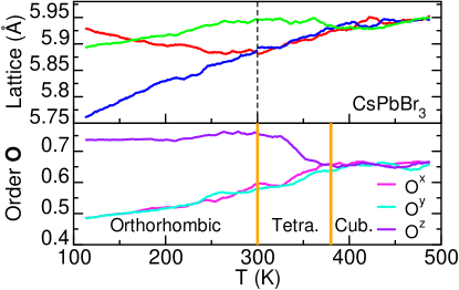
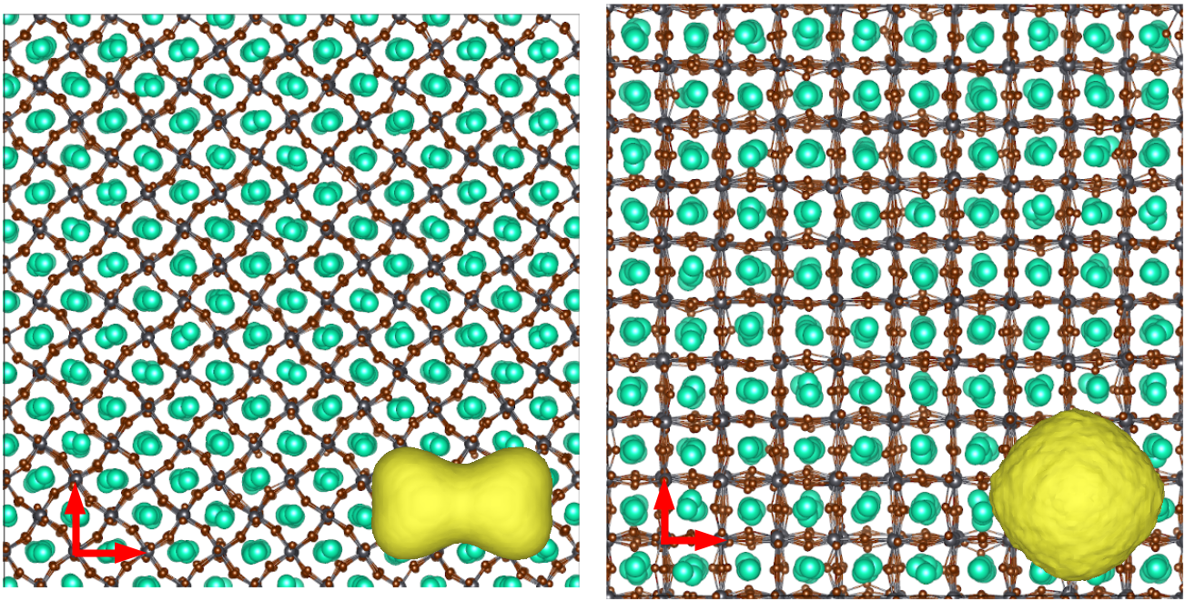
Figure 1: Lattice structure of CsPbBr₃ as function of temperature. Top: The lattice constants in pseudo-cubic representation and PbBr framework order parameter vector ($\mathbf{O}$) characterize a orthorhombic (T $<$ 300 K), tetragonal and cubic (T $>$ 380 K) perovskite phase. Data obtained from slow heating $NPT$-MD with the MLFFJinnouchi et al. (2019a). Bottom: Snapshots from the $8\times 8\times 8$ orthorhombic and $10\times 10\times 10$ cubic supercells during $NVT$-MD simulations at 150 K and 400 K, respectively. The unitcells are indicated by the red arrows. The yellow iso-surface shows the displacement of the Cs from the geometric center of the PbBr cages. The Supplementary Movie illustrates the ’rattling’ Cs⁺ cations in the two crystal phases.

II Computational Methods

II.1 Machine-Learning force-field molecular dynamics

An on-the-fly trained MLFF is used (in production mode, i.e. no new training) to run MD simulations for CsPbBr₃. The generation of this force field and its training parameters are described in detail in Ref.  Jinnouchi et al., 2019a. We briefly reiterate the most physically meaningful aspects. The MLFF is trained on total energies, forces and stress tensors obtained from DFT. The used algorithm automatically (on-the-fly) selects structures from the isothermal–isobaric ensemble by a Bayes error estimate. A variant of the GAP-SOAPBartók et al. (2010, 2013) method is used to describe the local atomic configuration for each atom. Within a cutoff radius of 6 Å (radial $\rho^{(2)}(r_{ij})$) and 5 Å (angular $\rho^{(3)}(r_{ij},s_{ik},\theta_{ijk})$) probability distributions are built by adding Gaussians with a width of 0.5 Å. The two-body descriptor $\rho_{i}^{(2)}$ of atom $i$ describes the probability of finding another atom $j$ at a distance $r_{ij}$. The three-body descriptor $\rho_{i}^{(3)}$ of atom $i$ describes the probability to find atom $j$ at a distance $r_{ij}$ while at the same time there is an atom $k$ at distance $s_{ik}$ from $i$, spanning an angle $\theta_{ijk}$ between the connection vectors $\mathbf{r}_{ij}$ and $\mathbf{s}_{ik}$. Note that in this implementation the two-body contribution ($j=k$) to $\rho_{i}^{(3)}$ is omitted, thereby creating two separable descriptorsLiu et al. (2021). The obtained distributions are projected onto spherical Bessel functions of the order 6 and 9 for the radial and angular part, respectively. The angular part is multiplied with spherical harmonics where the maximal angular momentum was set to $l_{max}=6$. The coefficients of the projections are gathered in the descriptor vector $\mathbf{X}_{i}$. A kernel-based regression method is applied to map the two descriptors to a local atomic energy

$$U_{i}=F[\rho_{i}^{(2)},\rho_{i}^{(3)}]=\sum_{i_{B}}^{N_{B}}w_{i_{B}}K(\mathbf{X}_{i},\mathbf{X}_{i_{B}}),$$ (1)

where $\rho_{i}^{(2)}$ and $\rho_{i}^{(3)}$ are the total two and three body descriptors of atom i. $N_{B}$ denotes the number of used local atomic reference configurations. The kernel is given by a polynomial function

$$K(\mathbf{X}_{i},\mathbf{X}_{i_{B}})=\frac{1}{2}(\mathbf{X}^{(2)}_{i}\cdot{}\mathbf{X}^{(2)}_{i_{B}})+\frac{1}{2}(\mathbf{X}^{(3)}_{i}\cdot{}\mathbf{X}^{(3)}_{i_{B}})^{4}.$$ (2)

On-the-fly training was performed during a $2\times 2\times 2$ supercell $NPT$-MD run in a stepwise manner. For 500 K, 370 K and 150 K, 100 ps long training runs were performedJinnouchi et al. (2019a). The DFT calculations use a plane-wave basis, the projector-augmented wave methodBlöchl (1994) and the SCANSun et al. (2015) density functional approximation. This density functional accurately describes the these types of lead-based halide perovskitesBokdam et al. (2017); Lahnsteiner et al. (2018). In total 572 DFT structure datasets were selected by the Bayesian error estimate during training, from which 187 (Pb), 1068 (Br) and 224 (Cs) local reference configurations are used. A comprehensive description of the on-the-fly MLFF generation implemented in the Vienna Ab-initio Simulation Package (VASP) is given in Ref. Jinnouchi et al., 2019b.

The MLFF was shown to predict phase-transition temperatures in close agreement with experimental observations, with predicted temperatures of $300$ K and $380$ K for the orthorhombic to tetragonal and the tetragonal to cubic transition, respectivelyJinnouchi et al. (2019a). These temperatures are based on the slow heating and cooling runs of supercells containing $6\times 6\times 6$ formula units. The change of the lattice parameters and change of the relative orientation of neighbouring PbBr octahedra while heating is shown in Fig. 1. These findings are in close agreement with experimental measurements based on variable temperature X-ray diffraction analysis showing phase transitions at $361$ K and $403$ KSarunas et al. (2020). The root-mean-square errors in energy, forces and stress between DFT and the MLFF over the total temperature interval are below 4 meV/atom, 0.05 meV/Å and 1 kBar, respectively. A detailed error analysis can be found in the supplementary material of Ref. Jinnouchi et al., 2019a. All of the above indicates that the constructed MLFF is an appropriate model to describe the CsPbBr₃ lattice dynamics.

In this work, large-scale simulations of CsPbBr₃ were done at $150$ K and $400$ K. The lattice constants for this simulations were extracted from Jinnouchi et.al.Jinnouchi et al. (2019a) and are reported in Table 1. For the orthorhombic simulation at $150$ K a unit cell containing 4 Pb, 4 Cs and 12 Br atoms was constructed. This unit cell was replicated $8\times 8\times 8$ times, containing in total 10,240 atoms. The $10\times 10\times 10$ cubic supercell was constructed from a simpler cubic unit cell containing 5 atoms. Hence, the cubic simulation contains in total 5,000 atoms. The time steps were adjusted to $10$ fs and $5$ fs for the orthorhombic and the cubic simulation, respectively. The two systems were equilibrated for $100$ ps. After this initialization 20 starting structures were taken with $100$ ps inbetween them, resulting in a total equilibration time of $2,100$ ps and 20 molecular dynamics runs per temperature. To obtain the trajectories required for our analysis every starting structure was propagated for $200$ ps in the microcanonical ensemble.

Table 1: Equilibrium unitcell lattice parameters of CsPbBr₃ in the microcanonical MD simulations. Parameters adapted from Ref. Jinnouchi et al., 2019a

Temperature [K]	$a$ [Å]	$b$ [Å]	$c$ [Å]
$150$	8.37	8.16	11.79
$400$	5.93	5.93	5.93

II.2 Notation

We represent crystals as supercells which are a periodic arrangement of unit cells. A sketch of a 2 dimensional $4\times 4$ supercell is shown in Fig 2 on the left hand side.

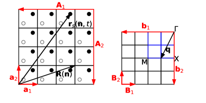
Figure 2: Left: A $4\times 4\times 4$ cubic primitive supercell in 2 dimensions. The vectors $\mathbf{a}_{i}$ denote the unit-cell, $\mathbf{A}_{i}$ are the vectors defining the created supercell, $\mathbf{R}(\mathbf{n})$ denotes the unit-cell positions, and $\mathbf{r}(\mathbf{n},t)$ are the coordinates of the atoms residing in the unit-cells.
Right: Reciprocal cell of the cubic cell. The vectors $\mathbf{b}_{i}$ denote the reciprocal primitive lattice. The blue squares are in the first irreducible Brillouin zone of the supercell spanned by $\mathbf{A}_{i}$. The vectors $\mathbf{B}_{i}$ are the reciprocal vectors of the supercell. The points named X, M and $\Gamma$ are the high symmetry points of a cubic primitive lattice in the considered plane.

To identify one of the unit-cells making up the supercell the vector $\mathbf{R}(\mathbf{n})$ is used. In 3 dimensional space the vector $\mathbf{R}(\mathbf{n})$ is given by

$$\mathbf{R}(\mathbf{n})=n_{1}\mathbf{a}_{1}+n_{2}\mathbf{a}_{2}+n_{3}\mathbf{a}_{3},$$ (3)

where $\mathbf{a}_{i}$ are the lattice vectors spanning the unit-cell. The index vector $\mathbf{n}$ uniquely determines a unit-cell within the supercell. The individual atoms residing in a unit-cell can be identified by the vector $\mathbf{r}_{s}(\mathbf{n},t)$. The time dependence $t$ of the atomic positions comes from the molecular dynamics approach. The index $s$ on the vector denotes the atom index within the unit-cell. The total number of atoms in a unit-cell is $\nu$. The lattice vectors of the supercell are given by $\mathbf{A}_{i}=N_{i}\mathbf{a}_{i}$ and $N{i}$ is the number of repeating unit-cells in the 3 different directions. For every supercell there exists a reciprocal cell. An example of a reciprocal cell is shown on the right-hand side of Fig 2. The reciprocal unit-cell vectors $\mathbf{b}_{i}$ are

$$\mathbf{b}_{1}=\frac{2\pi}{\mathbf{a}_{1}(\mathbf{a}_{2}\times\mathbf{a}_{3})}\mathbf{a}_{2}\times\mathbf{a}_{3}$$

$$\mathbf{b}_{2}=\frac{2\pi}{\mathbf{a}_{1}(\mathbf{a}_{2}\times\mathbf{a}_{3})}\mathbf{a}_{3}\times\mathbf{a}_{1}$$ (4)

$$\mathbf{b}_{3}=\frac{2\pi}{\mathbf{a}_{1}(\mathbf{a}_{2}\times\mathbf{a}_{3})}\mathbf{a}_{1}\times\mathbf{a}_{2}.$$

The reciprocal supercell is spanned by the vectors $\mathbf{B}_{i}=\frac{1}{N_{i}}\mathbf{b}_{i}$ where the number of repeating reciprocal unit-cells has to match the $N_{i}$ from the real space supercell. The sampled Brillouin zone is shown in Fig 2 on the right hand side by the blue square. Within the first Brillouin zone we define reciprocal wave vectors

$$\mathbf{q}=\frac{l_{1}}{N_{1}}\mathbf{b}_{1}+\frac{l_{2}}{N_{2}}\mathbf{b}_{2}+\frac{l_{3}}{N_{3}}\mathbf{b}_{3},$$ (5)

where the $l_{i}\in[0,-\frac{N_{i}}{2}]$ are a set of integers uniquely defining the accessible $\mathbf{q}$-points. To label the wave vectors in the result sections we use fractional coordinates $\frac{l_{i}}{N_{i}}$.

II.3 Phonon density of states computation

The phonon density-of-states (DOS) $f_{s}(\omega)$, for atom $s$ in the unit-cell is computed during an MD run from the VACF $f_{s}(t)$ given byDove (1993); Sun et al. (2014); Kneller and Hinsen (2001); Dickey and Paskin (1969)

$$f_{s}(t)=\frac{\left\langle\sum_{\mathbf{n}}\mathbf{v}_{s}(\mathbf{n},t^{\prime})\mathbf{v}_{s}(\mathbf{n},t^{\prime\prime})\right\rangle}{\langle\sum_{\mathbf{n}}\mathbf{v}_{s}(\mathbf{n},t^{\prime\prime})\mathbf{v}_{s}(\mathbf{n},t^{\prime\prime})\rangle},$$ (6)

where $\mathbf{v}_{s}(\mathbf{n},t^{\prime})$ is the 3-dimensional velocity of an certain atom $s$ in unit cell $\mathbf{n}$ at time t’. The time argument of the correlation function $f_{s}$ is given by $t=t^{\prime}-t^{\prime\prime}$, and the thermal average $\langle.\rangle$ is computed over the unit cells in the crystal for every atom $s$. The phonon DOS per atom $s$ is obtained by Fourier transforming Eq. (6)

$$f_{s}(\omega)=\int_{\mathbb{R}}f_{s}(t)e^{-i\omega t}dt.$$ (7)

From this, the total DOS is given as the mass-weighted sum of the individual atomic contributions

$$F(\omega)=\sum_{s=1}^{\nu}\sqrt{m_{s}}f_{s}(\omega).$$ (8)

The sum runs over all atoms with masses $m_{s}$ in the unit cell. Capital letters denote quantities reweighed by the square-root of the mass. The phonon DOS is expected to give peaks at all resonant frequencies $\omega$ of the studied system. The VACF does not contain any $\mathbf{q}$ resolution and can therefore be considered as a sum over the contributions arising from different $\mathbf{q}$.

II.4 $\mathbf{q}$-resolved velocity autocorrelation functions

A $\mathbf{q}$-resolved form of the VACF ($\mathbf{q}$-VACF) is computed analogous to Sec. II.3. This is done by Fourier transforming the mass weighed velocity field to $\mathbf{q}$-space

$$\mathbf{V}_{s}(\mathbf{q},t)=\sum_{\mathbf{n}}\sqrt{m}_{s}\mathbf{v}_{s}(\mathbf{n},t)e^{i\mathbf{q}\mathbf{r}_{s}(\mathbf{n},t)},$$ (9)

Then Eq. (9) is self-correlated and the temporal Fourier transform is computed

$$H_{s}(\mathbf{q},\omega)=\int\mathbf{V}_{s}(\mathbf{q},t^{\prime})\mathbf{V}_{s}(\mathbf{-q},t^{\prime\prime})e^{-i\omega t}dt,$$ (10)

with $t=t^{\prime}-t^{\prime\prime}$ and $\text{d}t$ the corresponding differential. The power spectrum of the so obtained function is a $\mathbf{q}$-resolved form of the phonon DOS Dong-Bo et al. (2014); Sun et al. (2014, 2010b); Ladd et al. (1986).

II.5 Projected velocity autocorrelation functions

The $\mathbf{q}$-VACF is decomposed by a set of phonon eigenvectors $\mathbf{e}_{s,\alpha}(\mathbf{q})$ Sun et al. (2010a); Dong-Bo et al. (2014, 2017); Sun et al. (2014); Kneller and Hinsen (2001), where $\alpha$ denotes the branch index. The branch index $\alpha$ goes from 1 to 3 times the number of atoms $\nu$ in the unit-cell. Details about the definition of the phonon eigenvectors can be found in Appendix A. The decomposition is done by projecting the velocities $\mathbf{v}_{s}(\mathbf{n},t)$ onto the phonon polarization vectors $\mathbf{e}_{s,\alpha}(\mathbf{q})$ $(\in\mathbb{R}^{3})$, with PVACF in $\mathbf{q}$ space is obtained by a spatial Fourier transform Sun et al. (2010a); Dong-Bo et al. (2014, 2017); Sun et al. (2014)

$$G_{\alpha}(\mathbf{q},t^{\prime}) =\sum_{\mathbf{n}}\sum_{s}\left(\left(\sqrt{m_{s}}\mathbf{v}_{s}(\mathbf{n},t^{\prime})\right)\mathbf{e}_{s,\alpha}(\mathbf{q})\right)e^{i\mathbf{q}\mathbf{r}_{s}(\mathbf{n},t^{\prime})}$$

$$=\sum_{\mathbf{n}}\sum_{s}\left(\mathbf{V}_{s}(\mathbf{n},t^{\prime})\mathbf{e}_{s,\alpha}(\mathbf{q})\right)e^{i\mathbf{q}\mathbf{r}_{s}(\mathbf{n},t^{\prime})}$$ (11)

The symbol $\mathbf{V}_{s}(\mathbf{n},t)$ denotes the mass-weighted velocity vector. The self-correlation of Equation (11),

$$G_{\alpha}(\mathbf{q},t)=\sum_{\mathbf{n},s,\mathbf{n}^{\prime}} \left[\mathbf{V}_{s}(\mathbf{n},t^{\prime})\mathbf{e}_{s,\alpha}(\mathbf{q})\right]\left[\mathbf{V}_{s}(\mathbf{n}^{\prime},t^{\prime\prime})\mathbf{e}_{s,\alpha}(\mathbf{q})\right]$$

$$\times e^{i\mathbf{q}\left(\mathbf{r}_{s}(\mathbf{n},t^{\prime})-\mathbf{r}_{s}(\mathbf{n}^{\prime},t^{\prime\prime})\right)},$$ (12)

results in a VACF in $\mathbf{q}$ space projected onto the phonon polarization vectors $\mathbf{e}_{s,\alpha}(\mathbf{q})$, with time variable $t=t^{\prime}-t^{\prime\prime}$. A temporal Fourier transform from time $t$ to frequency space $\omega$ is done for Eq. (12)

$$G_{\alpha}(\mathbf{q},\omega)=\int_{\mathbb{R}}G_{\alpha}(\mathbf{q},t)e^{-i\omega t}dt.$$ (13)

By computing the power spectrum $|G_{\alpha}(\mathbf{q},\omega)|^{2}$ of Eq. (13) we obtain the intensity of a particular phonon eigenmode $\mathbf{e}_{\alpha,s}(\mathbf{q})$ on the ($\mathbf{q},\omega$) grid. The positions of the peaks are related to the renormalized phonon eigen-frequencies $\tilde{\omega}_{\alpha}(\mathbf{q})$ of the states $\mathbf{e}_{\alpha}(\mathbf{q})$.

The power spectrum $|G_{\alpha}(\mathbf{q},\omega)|^{2}$ has to show a single, well-defined Lorentzian shaped peak to make physical sense. This means that the eigenvector represents a phonon mode with a particular frequency $\tilde{\omega}_{\alpha}(\mathbf{q})$ and a phonon lifetime inversely proportional to the peak width Dong-Bo et al. (2014); Sun et al. (2014, 2010b); Ladd et al. (1986). The eigenvectors are obtained by a Phonopy Togo and Tanaka (2015) calculation. The harmonic phonon calculations were done on $10\times 10\times 10$ supercells for the cubic and $8\times 8\times 8$ for the orthorhombic system. The ground state structures on which the harmonic approximation is computed were relaxed with an energy difference criterion of $10^{-4}eV$. The FORTRAN implementations of the $\mathbf{q}$-VACF and the PVACF were added to our DSLEAP-code which open-source available, see Sec. V. The correlation functions are computed piecewise in time such that it is possible to read the trajectory file structure by structure. We are aware that there are several codes available for computing the PVACF and extracting renormalized phonon frequencies such as the DynaPhoPyCarreras et al. (2017) code, the phq Zhang et al. (2019) code or the ALAMODE Tadano et al. (2014) code, giving the possibility to study anharmonic phonon frequencies. These codes are user-friendly and handy, but they are not applicable to the here shown simulations since they read in the whole trajectory file at once, thereby overflowing the memory.

II.6 Determining Cs⁺ rattling frequency

The Cs⁺ cations are locked in Pb-Br cages to which they are bound by electrostatic interactions. The Cs⁺ cations are expected to ’rattle’ in their octahedra at finite temperature. This rattling of the Cs⁺ ions was proposed as one of the mechanisms responsible for the low phonon lifetimes reported for this materialLee et al. (2017a); Wang et al. (2018b); Simoncelli et al. (2019a); Songvilay et al. (2019). To determine the rattling motions in terms of a self-correlation function, the time-dependent displacement vector $\mathbf{d}_{\text{Cs}}(t)$ of the Cs⁺ cation from the geometric center (GC) of its surrounding lead framework is used. Therefore, the first step is to determine the eight nearest lead atoms surrounding each Cs⁺ ion. Then the GC of the lead cube is computed $\mathbf{r}_{\text{GC}}(t)$. Thereafter, the displacement vector $\mathbf{d}_{\text{Cs}}(t)$ is defined as

$$\mathbf{d}_{\text{Cs}}(t)=\mathbf{r}_{\text{Cs}}(t)-\mathbf{r}_{\text{GC}}(t).$$ (14)

and its self-correlation function is given by

$$c_{Cs}(t_{1}-t_{2})=\mathbf{d}_{\text{Cs}}(t_{1})\mathbf{d}_{\text{Cs}}(t_{2}).$$ (15)

This results in a self-correlation function for the Cs⁺ motion relative to its GC position

$$c_{Cs}(t_{1}-t_{2})=\mathbf{d}_{\text{Cs}}(t_{1})\mathbf{d}_{\text{Cs}}(t_{2}).$$ (16)

Equation (16) is computed for the orthorhombic and the cubic simulation of CsPbBr₃. The obtained signals are then analyzed by means of a Fourier transform. The power spectra of the Fourier transformed signals $c_{Cs}(\omega)$ are fitted by a Lorentzian function

$$[I,\omega_{0},\Gamma] =\operatorname*{arg\,min}_{I,\omega_{0},\Gamma}\left(I\left[\frac{\Gamma^{2}}{(\omega-\omega_{0})^{2}+\Gamma^{2}}\right]\right.$$

$$\qquad\qquad\qquad\qquad\left.-|c_{Cs}(\omega)|^{2}\right)^{2}.$$ (17)

In Section III.1 we show that there are two separable decorrelation processes at play, one of which we assign to rattling.

II.7 Computation of thermal averages

For the computation of the thermal averages we apply two kinds of averages. First a time average over different starting times within a single trajectory, denoted by $\langle.\rangle_{\text{time}}$ is computed. Then the power spectra are computed and averaged over different molecular dynamics runs, resulting in a thermal average denoted by $\langle.\rangle_{\text{Traj}}$. To formalize this process we will illustrate it for an example function $h_{\alpha}(\mathbf{q},t)$. This function can be considered as any of the presented correlation functions, such as functions  6,10, 12 and 16. The time average of the correlation functions is computed by

$$\langle h_{\alpha}(\mathbf{q},t)\rangle_{\text{time}}=\frac{1}{N_{T}}\sum_{j=0}^{N_{T}-1}h_{\alpha}(\mathbf{q},t-\Delta tj),$$ (18)

with $\Delta t=\frac{T}{2(N_{T}-1)}$ for $N_{T}>1$. $N_{T}$ is chosen such that the time window after which a new starting configuration is sampled results in $\Delta t=50$ fs for both the cubic and the orthorhombic system. This results in 200 starting configurations per trajectory. The obtained time averaged function is Fourier transformed and the power spectrum is computed

$$\left|\langle h_{\alpha}(\mathbf{q},\omega)\rangle_{\text{time}}\right|^{2}=\left|\int_{-\infty}^{\infty}\langle h_{\alpha}(\mathbf{q},t)\rangle_{\text{time}}e^{-i\omega t}dt\right|^{2}.$$ (19)

The power spectrum is now averaged over the 20 simulated trajectories per perovskite phase

$$\left\langle\left|\langle h_{\alpha}(\mathbf{q},\omega)\rangle_{\text{time}}\right|^{2}\right\rangle_{\text{Traj}} =$$

$$\left\langle\left|\int_{-\infty}^{\infty}\langle h_{\alpha}(\mathbf{q},t)\rangle_{\text{time}}e^{-i\omega t}dt\right|^{2}\right\rangle_{\text{Traj}}.$$ (20)

During the analysis we also checked if the results would differ when first computing the trajectory average $\langle\rangle_{\text{Traj}}$ and then computing the Fourier transform and it’s power spectrum. If the trajectories are long enough the order of the computation does not matter and the two approaches result in the same spectral densities.

II.8 Renormalized eigenfrequency determination

From Equation (13) signals in frequency space $\omega$ are obtained for every phonon branch $\alpha$ and $\mathbf{q}$ vector. To obtain renormalized phonon frequencies $\tilde{\omega}_{\alpha}(\mathbf{q})$ Lorentzian functions are fitted to Eq. (13). Three parameter Lorentzians are used, one parameter to control the height ($I$), one parameter for the width ($\Gamma$) and a frequency parameter ($\omega_{0}$) equivalent to the renormalized frequency ($\tilde{\omega}_{\alpha}(\mathbf{q})$). The fitting procedure is described by,

$$[I_{\alpha}(\mathbf{q}),\tilde{\omega}_{\alpha}(\mathbf{q}),\Gamma_{\alpha}(\mathbf{q})] =\operatorname*{arg\,min}_{I,\omega_{0},\Gamma}\left(I\left[\frac{\Gamma^{2}}{(\omega-\omega_{0})^{2}+\Gamma^{2}}\right]\right.$$

$$\qquad\qquad\qquad\qquad\left.-|\langle G_{\alpha}(\mathbf{q},\omega)\rangle|^{2}\right)^{2}.$$ (21)

The three parameter Lorentzian is fitted with a linear least-square error to the signals $|\langle G_{\alpha}(\mathbf{q},\omega)\rangle|^{2}$. The parameter $\Gamma$ is related to the full width at half maximum (FWHM) by $(\text{FWHM)}_{\alpha}=2\Gamma_{\alpha}$ from which the phonon lifetimes can be computed by Dong-Bo et al. (2017)

$$\tau_{\alpha}(\mathbf{q})=\frac{1}{\left(\text{FWHM}\right)_{\alpha}(\mathbf{q})}=\frac{1}{2\Gamma_{\alpha}(\mathbf{q})}.$$ (22)

III Results

III.1 Cs⁺ Rattling in CsPbBr₃

Figure 3: Averaged self-correlation function of the displacement vector connecting the Cs atom to the geometric center of the surrounding PbBr cage.

Figure 1 shows that every $Cs^{+}$ cation in the CsPbBr₃ perovskite is surrounded by a lead bromide framework. Since the $Cs^{+}$ cations are only weakly bound to the framework by electrostatic interactions the $Cs^{+}$ ions will undergo rattling motions at finite temperature. The exact nature of these dynamics is unclear. We study the rattling motions of the $Cs^{+}$ cations by analysing the local order parameter described in section II.6. The Cs rattlers scattering with phonons that propagate through the crystal might be a possible explanation for the low phonon lifetimes Lee et al. (2017a); Wang et al. (2018b). We have calculated the displacement vector, see Eq. (14), of the $Cs^{+}$ with respect to the (geometric center) GC of the surrounding eight Pb atoms. Iso-surfaces of the 3-dimensional distributions of these vectors are shown in yellow color in Fig. 1 (bottom). Its self-correlation function is computed and is shown in Figure 3(a) for the cubic and orthorhombic phase. In the orthorhombic phase, the function converges to a plateau above zero. This shows that the $Cs^{+}$ cations at 150 K rattle around a fixed point away from the GC. At 400 K the $Cs^{+}$ displacement decorrelates completely, indicating that the $Cs^{+}$ rattles around the GC.

Figure 3(b) shows the Fourier transforms of the time signals. There are two underlying decorrelation processes: First, there is a random thermal motion (Brownian-like) of the Cs⁺ around its actual position described by an exponential function $e^{-kt}$Kubo and Hashitsume (1978). Secondly, a repositioning within the occupied lead cube to which we assign the rattling dynamics, described by $\text{cos}(\omega t)$. The related frequencies were estimated by fitting the results in the time domain (Eq. 16) of the cubic $400$ K simulation with $e^{-kt}\text{cos}(\omega t)$.

In the frequency domain, the parameter $k$ of the exponential is related to the width $\Gamma$ of the Lorentzian in Equation (17), and $\omega$ of the cosine is related to $\omega_{0}$. Therefore, the position $\omega_{0}$ of the Lorentzian describes the rattling frequency of the Cs⁺ cations.

The fitted function shown by the dashed lines in Fig. 3(b) assigns very similar rattling frequencies of $0.81$ THz and $0.79$ THz for the orthorhombic and the cubic phase, respectively. This shows that the rattling period is $\sim{}1.2$ ps. There also is a smaller peak in the orthorhombic phase at 1.9 THz. This rattling frequency is not visible in the cubic phase. The random thermal motion is faster, roughly $2.5$ THz, and similar in both phases. To illustrate the rattling motions two movies for the orthorhombic and the cubic phase were created and added as Supplementary Movie. For a better visualization of the rattling motions, a period of 0.4 ps has been set as the window size for a running average over two $NVE$ trajectories of 100 ps. In the following sections we will study the lattice dynamics of CsPbBr₃ and attempt to decompose them by means of a set of phonon eigenstates.

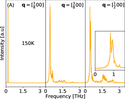
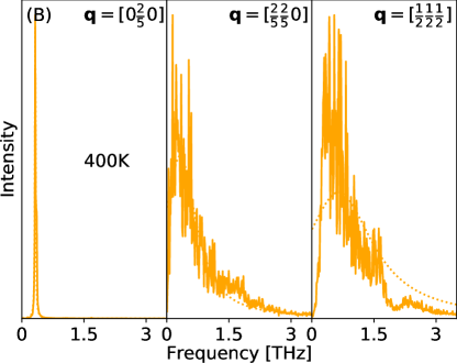
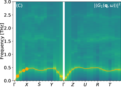
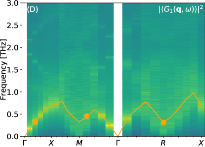
Figure 4: PVACFs of three selected $\mathbf{q}$-points projected on the eigenvectors of the first acoustic mode ($\alpha=1$) for (A) the orthorhombic phase at $150$ K and (B) cubic phase at 400 K. The solid lines show $|\langle G_{1}(\mathbf{q},\omega)\rangle|^{2}$ and the dotted-dashed orange lines shows Lorentzian fitting. $|\langle G_{1}(\mathbf{q},\omega)\rangle|^{2}$ along the full $\mathbf{q}$-point path obtained for (C) 150 K and (D) 400 K. Orange circles denote renormalised frequencies $\tilde{\omega}_{1}(\mathbf{q})$ corresponding to the peaks in (A,B) (from left to right).

III.2 The non-Lorentzian peak problem

When fitting the spectral densities obtained by Eq (13) a problem with the peak shape appears, which indicates the strong anharmonicity of the interaction potential. This problem is visualised in Figure 4 for both the orthorhombic and cubic phase. Fig. 4(A) shows three peaks corresponding to the PVACFs projected on eigenvectors of the first acoustic branch ($\alpha=1$) at three selected $\mathbf{q}$-points in the 150 K orthorhombic phase. The solid lines are the $\langle G_{1}(\mathbf{q},\omega)\rangle$ PVACFs power spectra and the dotted lines are the Lorentzian fits. The spectral density of only $\alpha=1$ along the full high symmetry $\mathbf{q}$-path is shown in Fig. 4(C). The orange circles in the plot are the renormalised frequencies $\tilde{\omega}_{1}(\mathbf{q})$ corresponding to the peaks shown in Fig. 4(A). For the $\mathbf{q}=\left[\frac{1}{8}\,\,0\,\,0\right]$ peak a Lorentzian with a well-defined eigenfrequency $\tilde{\omega}_{1}$ and linewidth $\Gamma_{1}$ can be fitted. For the $\mathbf{q}=\left[\frac{3}{8}\ 0\ 0\right]$ peak resonances appear as side peaks at higher frequencies in the spectrum. At $\mathbf{q}=\left[\frac{1}{2}\,\,0\,\,0\right]$ the power spectrum splits into two maxima emphasized by the inset of Fig 4(A). The fitting results in a Lorentzian engulfing both of the peaks. A well-defined weakly-interacting phonon quasi-particle should not show double peak signalsDong-Bo et al. (2014); Sun et al. (2014, 2010b); Ladd et al. (1986); Lu et al. (2017).

Also at 400 K in the cubic phase, the peak problem appears as shown in Figures 4(B,D). As before, only the acoustic branch $\alpha=1$ is shown in Figures 4(D). The $[0\ \frac{2}{5}\ 0]$ peak shows a well-defined phonon signal and can be fitted with a Lorentzian line shape. This is not the case for the peaks related to the slightly-off-M point $\mathbf{q}=\left[\frac{2}{5}\,\,\frac{2}{5}\,\,0\right]$ and R-point $\mathbf{q}=\left[\frac{1}{2}\,\,\frac{1}{2}\,\,\frac{1}{2}\right]$. According to Ref. Reissland (1973) a well-defined phonon has to satisfy the following inequality,

$$\tilde{\omega}_{\alpha}(\mathbf{q})\tau_{\alpha}(\mathbf{q})>1,$$ (23)

where $\tilde{\omega}_{\alpha}(\mathbf{q})$ is the renormalized frequency and $\tau_{\alpha}(\mathbf{q})$ is the phonon lifetime. The phonons of the first acoustic branch with wave vectors $\mathbf{q}=\left[\frac{2}{5}\ \frac{2}{5}\ 0\right]$ and $\mathbf{q}=\left[\frac{1}{2}\ \frac{1}{2}\ \frac{1}{2}\right]$ do not satisfy this criterion and therefore don’t form a well-defined state. Additionally, the form of the peaks deviates from the Lorentzian shape and would be better described by a skewed Gaussian distribution. Therefore, also in this type of peak, the PVACF approach with harmonic eigenvectors can not be applied in the strict sense of inequality (23).

Summarizing, phonons in CsPbBr₃ show many resonances with other phonon branches. Already in the spectral densities related to the first acoustic mode such resonances appear, as shown in Fig. 4. They show structure or high intensities not only for the mean frequency, but also for a broad part of the frequency spectrum. The further away from $\Gamma$ and the closer to the Brillouin zone boundary, the phonon quasiparticle in terms of the PVACF picture becomes hardly applicable.

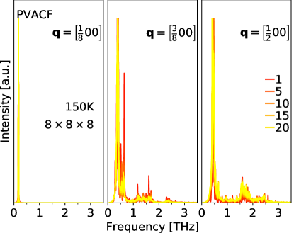
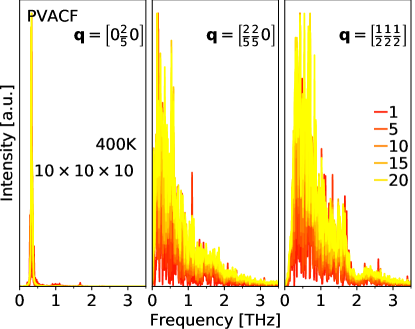
Figure 5: Convergence of the PVACF_α=1 power spectrum. The linear color scale of the curves depicts the number of trajectories, used for the average. Red is a single trajectory and yellow is an average over all 20 trajectories. Convergence of the signals for the orthorhombic ($8\times 8\times 8$) structure (top), and for the cubic ($10\times 10\times 10$) phase (bottom).

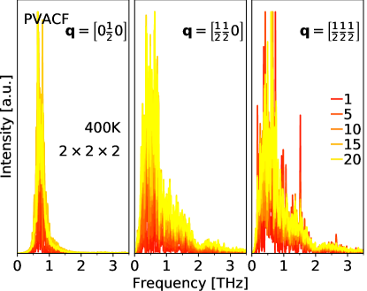
Figure 6: Convergence of the PVACF_α=1 power spectrum in a cubic $2\times 2\times 2$ simulation at 400K. Color scheme as in Fig. 5.

III.3 Convergence of the correlation functions

Before we start analysing the rest of the phonon spectrum (i.e. $\alpha\geq{}1$), we want to establish that our spectra are converged with respect to simulation time. In Figure 5 the simulation time convergence of the PVACF is shown for for $\alpha=1$ and the same $\mathbf{q}$-points as considered in Fig. 4. We are restricting our convergence analysis on the PVACF under the assumption that if the individual phonon branches are converged so has to be the $\mathbf{q}$-VACF which is a sum over the branch index $\alpha$. The orthorhombic simulations are shown in the upper panel and the cubic results are depicted in the lower panel. The color of the lines denote the number of independent (200 ps long) trajectories over which the average was computed. Each starting structure and the related velocities of a trajectory were taken from a well-equilibrated $NVT$ ensemble. From red to yellow the curves show averages taken over 2, 4 to 20 $NVE$ trajectories. The power spectra converge within the available amount of data of the PVACF. This can be seen because the double peak behaviour for the orthorhombic structure and the broad skewed distributions for the cubic structures remain in the PVACF, but are getting smoother. Notice the resonance peak intensities in Fig 5 at $\mathbf{q}=[\frac{3}{8}00]$ diminish during convergence. This indicates that a large amount of data is needed to obtain correct peak intensities. We also note that in the PVACF, peaks forming well-defined phonons converge faster than the more deformed peaks which experience stronger phonon-phonon interactions.

To test the influence of our large simulation box, similar simulations were done for a small $2\times 2\times 2$ structure at 400 K covering only $\frac{1}{125}$ of the volume of the large box. This is the typical dimension of the simulation box used in first-principles based MD simulations Guo et al. (2017); Klarbring et al. (2020); Chai et al. (2003); Dong-Bo et al. (2017, 2014); Sun et al. (2014). The convergence results for the high symmetry $\mathbf{q}$-points are shown in Figure 6. Also for this system size the spectra converge within the available amount of data. A comparison between the PVACF at 400 K in the $2\times 2\times 2$ (Fig. 6) and the $10\times 10\times 10$ (Figure 5) supercell at the $[\frac{1}{2}\frac{1}{2}\frac{1}{2}]$ $\mathbf{q}$-point shows equivalent signals for this $\mathbf{q}$-point. Only the relative noise in the case of the $2\times 2\times 2$-cell is slightly larger. This is a direct result of the smaller amount of samples when simulating a $2\times 2\times 2$-cell for the same amount of time.

In Fig. 7 a comparison between the power spectra of the first phonon branch in the $2\times 2\times 2$ and $10\times 10\times 10$ cubic phase is shown. Both boxes exhibit a narrow multi-peak signal $\mathbf{q}=[0\frac{1}{2}0]$, showing agreement between the box sizes for this $\mathbf{q}$-point. For $\mathbf{q}=[\frac{1}{2}\frac{1}{2}0]$ and $\mathbf{q}=[\frac{1}{2}\frac{1}{2}\frac{1}{2}]$, differences between the $2\times 2\times 2$ and the $10\times 10\times 10$ are visible. For both $\mathbf{q}$-points the peaks are narrower in the $10\times 10\times 10$ box. For $\mathbf{q}=[\frac{1}{2}\frac{1}{2}0]$ the fitted line widths ($\Gamma_{\alpha}(\mathbf{q}))$ are $\sim 0.40$ THz in the large box and $\sim 0.46$ THz in the small box. For $\mathbf{q}=[\frac{1}{2}\frac{1}{2}\frac{1}{2}]$ a similar behaviour is observed, where the $10\times 10\times 10$-box gives a linewidth of $\sim 0.39$ THz and the small box $\sim 0.49$ THz. Most notably is the shift of the peak maximum to smaller frequencies in the larger box. For $\mathbf{q}=[\frac{1}{2}\frac{1}{2}0]$ the renormalized frequency in the $10\times 10\times 10$ box is $\sim 0.32$ THz and in the $2\times 2\times 2$ box it is $\sim 0.55$ THz, resulting in a frequency shift of $\sim 0.21$ THz. For $\mathbf{q}=[\frac{1}{2}\frac{1}{2}\frac{1}{2}]$ the renormalized frequency in the larger box is $\sim 0.31$ THz and $\sim 0.55$ THz in the small box, what gives a frequency shift of $\sim 0.24$ THz similar to the previous $\mathbf{q}$-point. For the remaining acoustic and optical states we observe that if the powerspectrum of $G_{\alpha}(\mathbf{q})$ exhibits a narrow peak then the $10\times 10\times 10$ and the $2\times 2\times 2$ box give equivalent results as in the case of $\mathbf{q}=[0\frac{1}{2}0]$. But for states that experience a higher degree of anharmonicity broader peaks and higher frequencies are obtained in the $2\times 2\times 2$ box compared to the $10\times 10\times 10$ box.

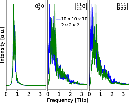
Figure 7: Comparison of the PVACF (${\alpha=1}$) power spectrum for a $10\times 10\times 10$ (blue) and a $2\times 2\times 2$ (green) supercell in the 400 K cubic phase.

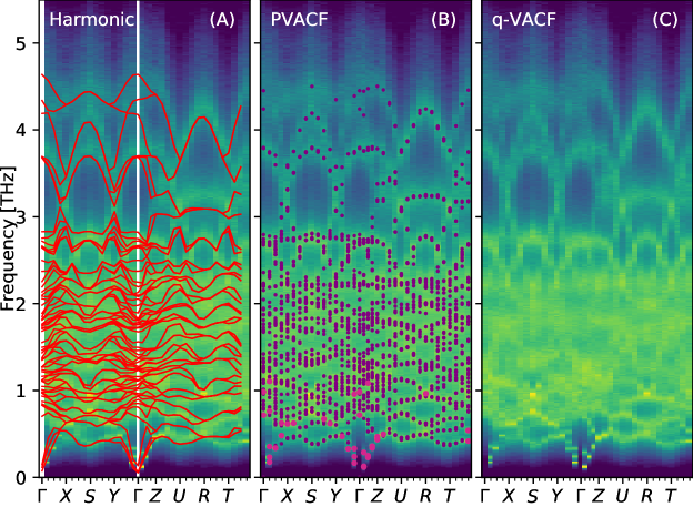
Figure 8: Phonon spectrum of orthorhombic CsPbBr₃ at 150 K. (a) The harmonic approximation is shown on top by the red lines. (b) the renormalized frequencies obeying inequality (23) and not showing multi-peaks are shown in dark-purple, renormalized frequencies obtained by ignoring multi-peaks and ignoring inequality (23) are shown by dark-purple dots. The background in (a) and (b) is the q-VACF as fully shown in (c).

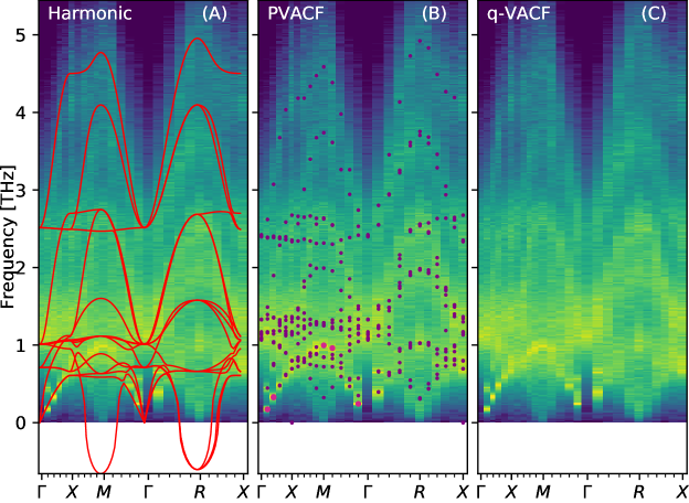
Figure 9: Phonon spectrum of orthorhombic CsPbBr₃ at 400 K. (a) The harmonic approximation is shown on top by the red lines. (b) the renormalized frequencies obeying inequality (23) and not showing multi-peaks are shown in dark-purple, renormalized frequencies obtained by ignoring multi-peaks and ignoring inequality (23) are shown by dark-purple dots. The background in (a) and (b) is the q-VACF as fully shown in (c).

Table 2: Renormalized eigenfrequencies $\tilde{\omega}_{\alpha}(\mathbf{q})$ and harmonic phonon eigenvectors at high symmetry points corresponding to modes with imaginary eigenfrequency in harmonic approximation.

Mode		M1	R1	R2	R3
$\tilde{\omega}$ [THz]		0.09	0.27	0.22	0.27
Pb	x	0.00	0.00	0.00	0.00
	y	0.00	0.00	0.00	0.00
	z	0.00	0.00	0.00	0.00
$\text{Br}_{x}$	x	0.00	0.00	0.00	0.00
	y	0.70	0.47	0.00	0.52
	z	0.00	-0.50	0.10	0.48
$\text{Br}_{y}$	x	-0.70	-0.47	-0.11	-0.52
	y	0.00	0.00	0.00	0.00
	z	0.00	-0.14	0.69	0.00
$\text{Br}_{z}$	x	0.00	0.51	0.11	-0.48
	y	0.00	0.15	-0.69	0.00
	z	0.00	0.00	0.00	0.00
Cs	x	0.00	0.00	0.00	0.00
	y	0.00	0.00	0.00	0.00
	z	0.00	0.00	0.00	0.00

III.4 CsPbBr₃ PVACF and q-VACF power spectra analysis

The dispersion relation for the orthorhombic phase including all acoustic and optical modes computed with the harmonic approximation is shown in Figure 8(A) by the red lines. The renormalized frequencies obtained from the PVACF are shown in Figure 8(B) by the dark and light-purple circles. The dark-purple points denote the PVACF power spectra for which the Lorentzian fitting was performed within the bounds of inequality (23) and without experiencing problems with multi-peak spectra. The light-purple points were obtained when ignoring the restrictions imposed by the used method. It is remarkable how few points in the bandstructure satisfy inequality (23) and show no resonance peak(s). Nevertheless, a comparison by eye of the so obtained renormalized frequencies to the colored background of the q-VACF seem to qualitatively agree with the dispersion obtained by the harmonic approximation. However, the average root-mean-square (rms) error computed between harmonic frequencies $\omega_{\alpha}(\mathbf{q})$ and the renormalized frequencies $\tilde{\omega}_{\alpha}(\mathbf{q})$ at the same $(\mathbf{q},\alpha)$ shows a large difference. Its large value of 0.3 THz indicates that the used fitting procedure has troubles with the many multi-peak features in the spectrum. This was exemplified by the inset of Fig 4(A).

In the q-VACF we can see overlapping flat bands up to a frequency range of around 3 THz. Overall, the broad and flat character of the bands suggests low phonon lifetimes and a high degree of anharmonicity, which is in agreement with previous studies Simoncelli et al. (2019b); Langian-Atkins et al. (2021); Guo et al. (2017); Lee et al. (2017b).

The analysis of the cubic phase at $400$ K is shown in Figure 9. The style of the figure is the same as that of Fig. 8. The renormalized frequencies $\tilde{\omega}_{\alpha}(\mathbf{q})$ obtained from the PVACF are depicted in Figure 9(B). The harmonic approximation Fig 9(A) shows imaginary eigenfrequencies for a single acoustic band at $\mathbf{q}=M$ and for all three acoustic modes at $\mathbf{q}=R$. The eigenvectors belonging to the imaginary eigenfrequencies are tabulated in table 2. These eigenmodes belong to polar rotational modes of the PbBr₆ octahedra around the enclosed lead atoms. Only Br atoms are participating in those stabilizing modes. By renormalizing the frequencies in the PVACF approach we obtain with real valued frequencies $\tilde{\omega}_{\alpha}(\mathbf{q})$. In this process the three-fold degeneracy of the acoustic mode at the R point is lifted.

As in the orthorhombic phase there are very few spectra that can be properly fitted, in the sense that it obeys the limits of inequality (23). Both the harmonic approximation and the PVACF show flat and close lying bands between 0.5 and 1.5 THz. The rms error between the harmonic approximation and the PVACF approach is 0.5 THz, i.e. slightly larger to the orthorhombic phase, what is expected for higher temperatures. The MD approach shows phonon mode softening for the two highest lying optical bands, compared to the harmonic approximation. The q-VACF is shown in Figure 9(C) and exhibits an overlapping band spectrum over the whole frequency region with only little structure. This indicates a high degree of anharmonicity in the underlying potential.

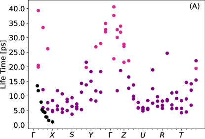
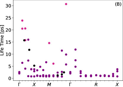
Figure 10: Acoustic phonon ($\alpha=1,2,3$) lifetimes for the (A) orthorhombic and the (B) cubic system obtained from the PVACF approach. The dark-purple circles depict the accurately fitted MD data. The light-purple circles represent peaks that were fitted by violating the proper phonon picture. The black circles show experimental phonon lifetimes of Ref. Songvilay et al. (2019).

III.5 Acoustic phonon lifetimes a comparison to experiment

The phonon lifetimes for the three acoustic modes were obtained by Eq. (22) from the fitted PVACF line widths $\Gamma_{\alpha}(\mathbf{q})$. The results are shown in Figure 10. Meaningful lifetimes in terms of inequality (23) could only be obtained around the $\Gamma$ point, as shown by the light-purple circles. The lifetimes indicated by the dark-purple circles were obtained by ignoring inequality (23) and the resonance peaks. Figure 10(A) shows three points for every $\mathbf{q}$-point corresponding to the lifetimes of the acoustic branches $\alpha=1,2,3$ in the orthorhombic phase. Additionally, experimental data for the acoustic modes measured by Songvilay et.al.Songvilay et al. (2019) is shown by the black circles. The experimental values and the phonon lifetimes measured from MLFF MD are of the same order of magnitude, and show the same trend when moving away from $\Gamma$. Interestingly, the experiment was only able to resolve phonon lifetimes in roughly the regions of the $\mathbf{q}$-space where our approach was able to predict lifetimes in agreement with inequality (23). Figure 10(B) shows that the cubic phase has on average shorter acoustic phonon lifetimes. Also here, qualitative agreement with experimentSongvilay et al. (2019) is found for the acoustic modes along the $\Gamma{\rm-X}$ and $\Gamma{\rm-M}$ paths.

For both the orthorhombic and the cubic simulations meaningful results can only be obtained for acoustic phonons with low momentum, ie. close to the $\Gamma$ point. The average acoustic phonon lifetimes are significantly higher in the orthorhombic compared to the cubic phase. This was to be expected since the atoms experience a lower degree of anharmonicity, as their displacements from equilibrium are smaller at lower temperatures.

III.6 Atom type resolved power spectra

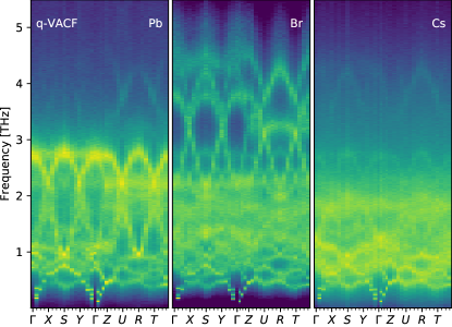
Figure 11: Atom resolved q-VACF for the (left) orthorhombic phase at 150 K and (right) cubic phase at 400 K.

As Figs.4, 8&9 have shown, the q-VACF and PVACF, show many highly anharmonic modes overlapping in the $[0.5,3]$ THz range. This makes the spectra difficult to disentangle. Therefore, a $\mathbf{q}$ and atom resolved form of q-VACF is shown in Figure 11. For both the cubic and the orthorhombic phase, the atom resolved q-VACF displays sharper features compared to the full q-VACF. A most remarkable feature is the broad flat band around $\sim$0.8 THz for the Cs⁺ cations extending over the whole Brillouin zone. This band is visible in both phases. In particular the q-VACF approach applied to the cubic phase visualizes this ’rattling band’. This band is nearly dispersionless around the rattling frequency (0.8 THz) obtained in Section III.1.

The phonon density of states and its atom decomposed form are computed and shown in Figure 12 for the orthorhombic and the cubic phase. We now clearly see that the low frequency peak of the Cs⁺ cations coincides with the rattling frequency. This Cs peak makes an important contribution to the total phonon DOS of the material. In the orthorhombic simulation there is another Cs peak visible at 1.9 THz, which is absent in the cubic simulations. This peak can not be assigned to the random thermal vibrations determined in Section III.1. This Cs peak is related to optical modes, and also shows the signatures of a dispersionless rattling band.

Furthermore, we can see the effect of the orthorhombic and cubic phase on the lead and bromide atoms. The DOS of the lead atoms show a peak at 2.75 THz, which is also visible in the total DOS. This peak is present in both phases, and experiences a red-shift of $\sim 0.1$ THz when going from orthorhombic to the cubic phase. In the bromide DOS of the orthorhombic phase multiple peaks are observed below 3 THz, which are smeared out in the cubic phase.

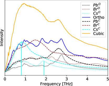
Figure 12: Phonon density of states obtained from unprojected velocity autocorrelation functions. The letter O in the legend denotes orthorhombic and C denotes cubic simulations. The vertical light-blue lines are the Cs rattling frequencies.

III.7 Disentangling phonon resonances in the acoustic branches

Before discussing the results and formulating our conclusions we will analyse the multi-peak spectra observed in the orthorhombic structure in more detail. We consider the three acoustic phonon branches at $\mathbf{q}=[\frac{1}{2}00]$, shown in Figure 13 as representatives. Phonon resonances can also occur between different $\mathbf{q}$-vectors, but as a simplification we will restrict ourselves to a single $\mathbf{q}$-point. All three acoustic signals show multi-peak behaviour. The positions marked with squares denote the locations of the renormalized eigenfrequencies. Beside the eigen-peaks every signal shows a number of resonant-peaks. The first acoustic phonon branch ($\alpha=1$) shows a multi-peak at $\sim 0.45$ THz. The second acoustic branch shows a very similar behaviour, with multi-peaks around the fitted frequency of $\sim 0.47$ THz. The two close lying peaks and the close lying eigen-frequencies of these two states indicate that they are very likely to resonate. In terms of the first acoustic branch we could argue that the peak higher in intensity is the phonon peak and the smaller one is the resonance with phonon branch 2. This argumentation can not be used for the second branch $\alpha=2$ because in this case the peaks are equal in magnitude and no unique choice what the main peak should be can be made. Moreover, both signals $\alpha=1$ and $\alpha=2$ show small resonances roughly at the positions of the main peak of the third acoustic branch ($\alpha=3$). The third acoustic branch has its eigenfrequency located at $\sim 0.6$ THz. It shows a resonant peak ($\sim 0.7$ THz) that can not be assigned to any of the acoustic branches at the same $\mathbf{q}$-point. All three acoustic branches show resonances with higher lying optical modes at the same $\mathbf{q}$-point with frequencies above $1.2$ THz. This indicates same $\mathbf{q}$-point interaction of phonon states with frequencies lying more than $1$ THz appart.

Figure 13: Power spectra of acoustic phonons measured in the orthorhombic phase at $\mathbf{q}=[\frac{1}{2}00]$. Circles show the maximum peak. The square symbols show the fitted peak maxima, i.e. the renormalized frequencies $\tilde{\omega}_{1}(\mathbf{q})$

From this analysis it follows that a decoupling of the atomic motions into independent phonon eigenmodes is not possible for this material. The potential is too anharmonic and the spacing between the phonon bands in the orthorhombic phase is too small to avoid resonances. Therefore it is not possible to decouple the system into independent modes. These phonon-phonon resonances are not only visible in the acoustic branch but are occurring throughout the whole phonon spectrum. Especially in regions of close lying bands and high crystal momentum $|\mathbf{q}|$, the power spectra show more resonances between phonon modes $\alpha$ and $\alpha^{\prime}$.

IV Discussion and Conclusion

In this work it was shown that large-scale MD simulations with accurate machine-learning potentials enable realistic simulations of the lattice dynamics of highly anharmonic materials such as the CsPbBr₃ perovskite. The importance of phonon-phonon interactions for CsPbBr₃ was reported in the computational work of Simonicelli et.al. Simoncelli et al. (2019b). Here, we showed that large supercell sizes are required in order to capture all phonon-phonon interactions properly. This was verified by our finite size analysis comparing the PVACF calculations of a $2\times 2\times 2$ and a $10\times 10\times 10$ supercell. This showed that depending on the phonon state the anharmonicity the phonon is experiencing can vary with the system size (Fig 7). The statistical convergence analysis showed that a large amount of MD samples are needed to properly converge the power spectra. The large-scale MD could not have been carried out with first-principles based MD in previous works Guo et al. (2017); Gehrmann and Egger (2019); Klarbring et al. (2020); Chai et al. (2003); Dong-Bo et al. (2017, 2014); Sun et al. (2014). Larger simulations would be computationally too expensive and only small supercells are tractable. The applied machine-learning approachJinnouchi et al. (2019a) combined with the here developed analysis code “DSLEAP” opens up the possibility to study anharmonic lattice dynamics by large-scale MD simulations and taking into account all degrees of anharmonicity. The extracted acoustic phonon lifetimes qualitatively agree with experimental results Songvilay et al. (2019); they are of the same order of magnitude and show similar $\mathbf{q}$-dependence. The phonon lifetimes are inversely proportional to their distance from $\Gamma$.

We conclude that it is not possible to decompose the lattice dynamics of CsPbBr₃ into a set of independent oscillators. Inequality 23 only holds for peaks close to the $\Gamma$ point in the orthorhombic and only for the acoustic modes close to the $\Gamma$ point in the cubic phase. This shows that phonon-phonon interactions play a major role in this system and cannot be ignored. Therefore we propose that the phonons in CsPbBr₃ have to be considered as a phonon-liquid and not as a weakly interacting gas. This can be clearly recognized by the strong resonances observed in the power spectra indicating coupled phonon states. We are using the term phonon-liquid as an analogy between phonons and particles in real space. If real space particles are very diluted, then their interactions can be neglected and they form a gaseous state. This is analogous to phonons in a harmonic solid. The phonons are only very weakly interacting and form a so called phonon gasReissland (1973). If the density of real space particles is raised, the interactions become important and we are talking about a liquid. The analogous behaviour in the phonon picture is a highly anharmonic crystal. The anharmonicities introduce strong phonon-phonon interactions that can not be ignored and hence we are talking about a phonon-liquid. The importance of phonon-phonon interactions was also recognized in Ref. Simoncelli et al. (2019b) and in the neutron scattering study of Ref. Langian-Atkins et al. (2021). Similar results were obtained in a combined experimental and theoretical work by Sharma et.al. for the MAPbI₃ perovskiteSharma et al. (2020). In this study we attempted to identify main and resonance peaks by comparing the acoustic phonon branches for a selected $\mathbf{q}$-point (see Fig. 13). The intensity of these resonant peaks can be used as a measure for the importance of the phonon-phonon interaction. In some cases the resonant peaks are nearly as intense as the main peak. These findings indicate a high degree of anharmonicity in the underlying potential.

In the literature the ultra-low thermal conductivity is partly attributed to ’rattling’ motions of the Cs⁺ cationsLee et al. (2017b); Simoncelli et al. (2019a). Rattling motions are also said to be responsible for low thermal conductivities in other materials as for example in sodium cobaltate Voneshen et al. (2013) or CuCrSe₂ Niedziela et al. (2019). The study of the Cs⁺ cation correlation function showed that rattling frequencies can be extracted from MD runs by the use of correlation functions of atomic displacements. A rattling frequency of $0.8$ THz and a faster random motion of roughly $2.5$ THz, characterizes this process. The atom decomposed $\mathbf{q}$-VACF show that rattling motions show only very weak dispersion. Therefore, we define rattling motions as a nearly dispersionless atomic oscillation with a broad frequency spectrum, but with a well defined average frequency.

The analysis of the dispersion curves has shown that the CsPbBr₃ is dynamically stabilized. Dynamic stabilization is indicated by imaginary modes in the harmonic approximation that can be renormalized by the PVACF approach to give positive frequencies. This finding is in agreement with the computational studies of Refs. Langian-Atkins et al. (2021); Guo et al. (2017); Gehrmann and Egger (2019). The modes responsible for the dynamic stabilization are the M and R points, and contain only motions of the Br atoms. These modes form the characteristic rotation and tilting pattern known to be important in many perovskite structures. For example, in the CaSiO₃ Sun et al. (2014) or MAPbI₃ Whalley et al. (2016); Sharma et al. (2020) perovskites.

Summarizing, we have shown that the phonon properties of such highly anharmonic materials as the CsPbBr₃ perovskite can be studied in large-scale MLFF MD simulations. Without large-scale MD there is no guarantee to obtain the converged power spectrum when working with VACF methods. The CsPbBr₃ perovskite has shown to form a phonon liquid when its dynamics are projected onto harmonic eigenmodes. Only the acoustic modes close to the $\Gamma$ point show well-behaved power spectra in the sense of inequality (23). The rattling motion was identified to be a nearly dispersionless movement of the Cs⁺ cations at an effective frequency of 0.8 THz within the accessible space formed by the PbBr₆ octahedra. Last, the dynamic stabilization is caused by collective octahedral tilting modes only involving displacements of Br atoms.

V Code Availability

Algorithms were implemented for computing the (P)VACF in large supercells with long MD trajectories. The open source analysis code: Dynamic Solids Large Ensemble Analysis Package (DSLEAP) as well as a manual can be downloaded from: GitHub.

VI Acknowledgements

The authors would like to thank Ryosuke Jinnouchi and Georg Kresse for stimulating discussions. We thank Max Rang for providing valuable feedback on the manuscript. We acknowledge funding by the Austrian Science Fund (FWF): P 30316-N27. Computations were partly performed on the Vienna Scientific Cluster VSC3. This work was sponsored by NWO Domain Sience for the use of supercomputing facilities.

Appendix A The Harmonic Approximation

Using the notation introduced in section II.2 and defining the displacement from the equilibrium position as $\mathbf{u}_{s}(\mathbf{n},t)$, for atom $s$ in unit-cell $\mathbf{n}$. The harmonic approach uses a quadratic potential to approximate the true potential, that is defined by the model describing the atomic interactions. The Lagrangian of the harmonic crystal is given byLandau and Lifschitz (2016)

$$L= \frac{1}{2}\sum_{\mathbf{n},s}m_{s}\dot{\mathbf{u}}^{2}_{s}(\mathbf{n},t)-$$

$$\frac{1}{2}\sum_{\mathbf{n},\mathbf{n}^{\prime}}\sum_{s,s^{\prime}}\mathbf{u}^{T}_{s^{\prime}}(\mathbf{n}^{\prime},t)\mathbf{\Lambda}_{s,s^{\prime}}(\mathbf{n}-\mathbf{n^{\prime}})\mathbf{u}_{s}(\mathbf{n},t),$$ (24)

where $\mathbf{\Lambda}_{s,s^{\prime}}(\mathbf{n}-\mathbf{n^{\prime}})$ is a $3\times 3$ matrix describing the coupling strength between a pair of atoms $s$ and $s^{\prime}$ located in unit cells $\mathbf{n}$ and $\mathbf{n}^{\prime}$. Because the coupling of the atoms only depends on their relative positions the argument of $\mathbf{\Lambda}_{s,s^{\prime}}$ is $\mathbf{n}-\mathbf{n^{\prime}}$ Landau and Lifschitz (2016). The velocities of the atoms are $\dot{\mathbf{u}}_{s}(\mathbf{n},t)$ and the masses of the atoms are given by $m_{s}$. From the Lagrangian the equations of motions can be obtained

$$m_{s}\ddot{\mathbf{u}}_{s}(\mathbf{n},t)=-\sum_{\mathbf{n}^{\prime},s^{\prime}}\mathbf{\Lambda}_{s,s^{\prime}}(\mathbf{n}-\mathbf{n}^{\prime})\mathbf{u}_{s^{\prime}}(\mathbf{n}^{\prime},t),$$ (25)

where $\ddot{\mathbf{u}}_{s}(\mathbf{n},t)$ is the acceleration of atom $s$ in unit-cell $\mathbf{n}$. A monochromatic plane wave Ansatz for the atomic displacements

$$\mathbf{u}_{s}(\mathbf{n},t)=\frac{1}{\sqrt{m_{s}}}\mathbf{e}_{s}(\mathbf{q})e^{i[\mathbf{q}\mathbf{r}_{s}(\mathbf{n},t)-\omega t]}$$ (26)

is used, where $\mathbf{e}_{s}(\mathbf{q})$ is the phonon polarization vector. Note that the polarization vector $\mathbf{e}_{s}(\mathbf{q}$ only depends on the atomic index $s$ and is therefore the same for same atom types in different unit-cells. Inserting the plane wave Ansatz (26) into the equation of motion (25) results in

$$\omega^{2}\sqrt{m_{s}}\mathbf{e}_{s}(\mathbf{q}) e^{i\mathbf{q}\mathbf{r}_{s}(\mathbf{n},t)}=$$ (27)

$$\sum_{\mathbf{n}^{\prime},s^{\prime}}\mathbf{\Lambda}_{s,s^{\prime}}(\mathbf{n}-\mathbf{n}^{\prime})\frac{1}{\sqrt{m_{s^{\prime}}}}\mathbf{e}_{s^{\prime}}(\mathbf{q})e^{i\mathbf{q}\mathbf{r}_{s^{\prime}}(\mathbf{n}^{\prime},t)}.$$

Dividing by $e^{i\mathbf{q}\mathbf{r}_{s}(\mathbf{n},t)}$ and carrying out the summation over $\mathbf{n}^{\prime}$ yields

$$\omega^{2}\sqrt{m_{s}}\mathbf{e}_{s}(\mathbf{q})=\sum_{s^{\prime}}\mathbf{\Lambda}_{s,s^{\prime}}(\mathbf{q})\frac{1}{\sqrt{m_{s^{\prime}}}}\mathbf{e}_{s^{\prime}}(\mathbf{q}),$$ (28)

where

$$\mathbf{\Lambda}_{s,s^{\prime}}(\mathbf{q})=\sum_{\mathbf{n^{\prime}}}\mathbf{\Lambda}_{s,s^{\prime}}(\mathbf{n}-\mathbf{n}^{\prime})e^{i\mathbf{q}[\mathbf{r}_{s^{\prime}}(\mathbf{n}^{\prime},t)-\mathbf{r}_{s}(\mathbf{n},t)]}.$$ (29)

Equation 28 is now divided by $\sqrt{m_{s}}$ and multiplied from the right by $e_{s^{\prime}}(\mathbf{q})$ to give

$$\mathbf{\Lambda}_{s,s^{\prime}}(\mathbf{q})\frac{1}{\sqrt{m_{s}m_{s^{\prime}}}}-\omega^{2}\delta_{s,s^{\prime}}=0$$ (30)

To obtain the solutions of this algebraic equation the determinant is taken

$$\text{det}|\mathbf{\Lambda}_{s,s^{\prime}}(\mathbf{q})\frac{1}{\sqrt{m_{s}m_{s^{\prime}}}}-\omega^{2}\delta_{s,s^{\prime}}|=0,$$ (31)

to obtain the $3\nu$ eigenvalues $\omega_{\alpha}(\mathbf{q})$, known as the dispersion relation. This implies that the eigenvectors must be indexed by the branch index to uniquely define them, giving $\mathbf{e}_{s,\alpha}(\mathbf{q})$.

The harmonic approximation decomposes the real crystal into a non-interacting phonon gas with phonon frequencies given by the dispersion relation $\omega_{\alpha}(\mathbf{q})$.

References

- Behler and Parrinello (2007) J. Behler and M. Parrinello, Phys. Rev. Lett. 98, 146401 (2007).
- Bartók et al. (2010) A. P. Bartók, M. C. Payne, R. Kondor, and G. Csányi, Phys. Rev. Lett. 104, 136403 (2010).
- Rupp et al. (2012) M. Rupp, A. Tkatchenko, K.-R. Müller, and O. A. von Lilienfeld, Phys. Rev. Lett. 108, 058301 (2012).
- Bartók et al. (2013) A. P. Bartók, R. Kondor, and G. Csányi, Phys. Rev. B 87, 184115 (2013).
- Wang et al. (2018a) Y. Wang, R. Lin, P. Zhu, Q. Zheng, Q. Wang, and D. Li, Nano Lett. 18, 2772 (2018a).
- Guo et al. (2017) Y. Guo, P. Xia, J. Gong, C. Stoumpos, C., M. McCall, K., C. B. Alexander, G., Z. H. G. D. J. Ma, Z., B. Ketterson, J., G. X. T. Kanatzidis, M., M. Chan, and R. Schaller, ACS Energy Letters 2, 2463 (2017).
- Eaton et al. (2016) S. W. Eaton, M. Lai, N. A. Gibson, A. B. Wong, L. Dou, J. Ma, L.-W. Wang, S. R. Leone, and P. Yang, Proc. Natl. Acad. Sci. U.S.A. 113, 1993 (2016).
- Chen et al. (2017) J. Chen, Y. Fu, L. Samad, L. Dang, Y. Zhao, S. Shen, L. Guo, and S. Jin, Nano Lett. 17, 460 (2017).
- Yuping and Giulia (2014) H. Yuping and G. Giulia, Chem. Mat. 26, 5394 (2014).
- Mettan et al. (2015) X. Mettan, A. Pisoni, J. Jacimovic, B. Nafradi, M. Spina, D. Pavuna, L. Forro, and E. Horvath, Journal of Physical Chemistry C 119, 11506 (2015).
- Filippetti et al. (2016) A. Filippetti, C. Caddeo, P. Delugas, and A. Mattoni, Journal of Physical Chemistry C 120, 28472 (2016).
- Hirotsu et al. (1974) S. Hirotsu, J. Harada, M. Irzumi, and K. Gesi, J. Phys. Soc. Jpn. 37, 1393 (1974).
- Jinnouchi et al. (2019a) R. Jinnouchi, J. Lahnsteiner, F. Karsai, G. Kresse, and M. Bokdam, Phys. Rev. Lett. 122, 225701 (2019a).
- Sarunas et al. (2020) S. Sarunas, S. Balciunas, M. Simenas, G. Usevicius, M. Kinka, M. Velicka, D. Kubicki, M. Castillo, A. Karabanov, V. Shvartsman, de Rosario S., V. Sablinskas, A. Salak, D. Lupascu, and J. Banys, J. Mater. Chem. A 8, 14015 (2020).
- Sun et al. (2010a) T. Sun, X. Shen, and B. Allen, Philip, Phys. Rev. B 82, 224304 (2010a).
- Dong-Bo et al. (2014) Z. Dong-Bo, T. Sun, and R. Wentzcovitch, Phys. Rev. Lett. 112, 058501 (2014).
- Sun et al. (2014) T. Sun, Z. Dong-Bo, and R. Wentzcovitch, Phys. Rev. B 89, 094109 (2014).
- Dong-Bo et al. (2017) Z. Dong-Bo, S. T. Allen, Phillip, B., and R. Wentzcovitch, Phys. Rev. B 96, 100302 (2017).
- Simoncelli et al. (2019a) M. Simoncelli, N. Marzari, and F. Mauri, Nature Phys. 15, 809 (2019a).
- Tadano and Saidi (2021) T. Tadano and A. Saidi, W., arXiv , 2103.00745 (2021).
- Marronier et al. (2017) A. Marronier, H. Lee, B. Geffroy, J. Even, Y. Bonnassieux, and G. Roma, J. Phys. Chem. Lett. 8, 2659 (2017).
- Yaffe et al. (2017) O. Yaffe, Y. Guo, L. Z. Tan, D. A. Egger, T. Hull, C. C. Stoumpos, F. Zheng, T. F. Heinz, L. Kronik, M. G. Kanatzidis, J. S. Owen, A. M. Rappe, M. A. Pimenta, and L. E. Brus, Phys. Rev. Lett. 118, 136001 (2017).
- Chai et al. (2003) J. Chai, D. Stroud, J. Hafner, and G. Kresse, Phys. Rev. B 67, 100302 (2003).
- Gehrmann and Egger (2019) C. Gehrmann and D. A. Egger, Nature Comm. 10, 3141 (2019).
- Klarbring et al. (2020) J. Klarbring, O. Hellman, A. Abrikosov, I., and I. Simak, S., Phys. Rev. Lett. 125, 045701 (2020).
- Landau and Lifschitz (2016) L. Landau and E. Lifschitz, Statistische Physik Teil 1 (Europa Lehrmittel, 2016).
- Togo and Tanaka (2015) A. Togo and I. Tanaka, Scr. Mater. 108, 1 (2015).
- Tadano et al. (2014) T. Tadano, Y. Gohda, and S. Tsuneyuki, J. Phys.: Condens. Matter 26, 225402 (2014).
- Carreras et al. (2017) A. Carreras, A. Togo, and I. Tanaka, Comp. Phys. Comm. 221, 221 (2017).
- Zhang et al. (2019) Z. Zhang, B. S. T. Zhang, D., and M. Wentzcovitch, R., Comp. Phys. Comm. 243, 110 (2019).
- Liu et al. (2021) P. Liu, C. Verdi, F. Karsai, and G. Kresse, Phys. Rev. Mat. 5, 053804 (2021).
- Blöchl (1994) P. E. Blöchl, Phys. Rev. B 50, 17953 (1994).
- Sun et al. (2015) J. Sun, A. Ruzsinszky, and J. P. Perdew, Phys. Rev. Lett. 115, 036402 (2015).
- Bokdam et al. (2017) M. Bokdam, J. Lahnsteiner, B. Ramberger, T. Schäfer, and G. Kresse, Phys. Rev. Lett. 119, 145501 (2017).
- Lahnsteiner et al. (2018) J. Lahnsteiner, G. Kresse, J. Heinen, and M. Bokdam, Phys. Rev. Mat. 2, 073604 (2018).
- Jinnouchi et al. (2019b) R. Jinnouchi, F. Karsai, and G. Kresse, Phys. Rev. B 100, 014105 (2019b).
- Dove (1993) D. Dove, Martin, Introduction to Lattice Dynamics (Cambridge University Press, 1993).
- Kneller and Hinsen (2001) R. Kneller, G. and K. Hinsen, J. Chem. Phys. 115, 11097 (2001).
- Dickey and Paskin (1969) M. Dickey, J. and A. Paskin, Phys. Rev. 188, 1407 (1969).
- Sun et al. (2010b) T. Sun, X. Shen, and P. Allen, Phys. Rev. B 82, 224304 (2010b).
- Ladd et al. (1986) J. C. Ladd, Anthony, B. Moran, and G. Hoover, William, Phys. Rev. B 34, 5058 (1986).
- Lee et al. (2017a) W. Lee, H. Li, A. B. Wong, D. Zhang, M. Lai, Y. Yu, Q. Kong, E. Lin, J. J. Urban, J. C. Grossman, and P. Yang, Proc. Natl. Acad. Sci. U.S.A. 114, 8693 (2017a).
- Wang et al. (2018b) Y. Wang, R. Lin, P. Zhu, Q. Zheng, Q. Wang, D. Li, and J. Zhu, Nano Lett. 18, 2772 (2018b).
- Songvilay et al. (2019) M. Songvilay, N. Giles-Donovan, M. Bari, G. Ye, Z., L. Minns, J., M. Green, G. Xu, M. Gehring, P., K. Schmalzl, D. Ratcliff, W., M. Brown, C., D. Chernyshov, W. Beek, S. Cochran, and C. Stock, Phys. Rev. Mat. 3, 093602 (2019).
- Kubo and Hashitsume (1978) R. Kubo and N. Hashitsume, Statistical Physics II (Springer-Verlag, 1978).
- Lu et al. (2017) Y. Lu, T. Sun, P. Zhang, P. Zhang, D.-B. Zhang, and R. Wentzcovitch, Phys. Rev. Lett. 118, 145702 (2017).
- Reissland (1973) A. Reissland, J., The Physics of Phonons (John Wiley and Sons Ltd., 1973).
- Simoncelli et al. (2019b) M. Simoncelli, N. Marzari, and F. Mauri, Nature Phys. 15, 809 (2019b).
- Langian-Atkins et al. (2021) T. Langian-Atkins, X. He, J. Krogstad, M., M. Pajerowski, D., L. Abernathy, D., M. N. X. Guangyong, N., X. Xu, Y. Chung, D., G. Kanatzidis, M., S. Rosenkranz, R. Osborn, and O. Delaire, Nature Mater. 20, 977–983 (2021).
- Lee et al. (2017b) W. Lee, H. Li, A. B. Wong, D. Zhang, M. Lai, Y. Yu, Q. Kong, E. Lin, J. J. Urban, J. C. Grossman, and P. Yang, Proc. Natl. Acad. Sci. U.S.A. 114, 8693 (2017b).
- Sharma et al. (2020) R. Sharma, Z. Dai, L. Gao, T. Brenner, L. Yadgarov, J. Zhang, Y. Rakita, R. Korobko, A. Rappe, and O. Yaffe, Phys. Rev. Mat. 4, 092401 (2020).
- Voneshen et al. (2013) J. Voneshen, D., K. Refson, E. Borissenko, A. P. A. Krisch, M. Bosak, E. Cemal, M. Enderle, M. Gutmann, M. Hoesch, L. Roger, M. Gannon, A. Boothroyd, S. Uthayakumar, D. Porter, and J. Goff, Nature Mater. 12, 1028 (2013).
- Niedziela et al. (2019) L. Niedziela, J., D. Bansal, F. May, A., L.-A. T. Ding, J., G. Ehlers, L. Abernathy, D., A. Said., and O. Delaire, Nature Phys. 15, 73 (2019).
- Whalley et al. (2016) L. Whalley, J. Skelton, M. Frost, and A. Walsh, Phys. Rev. B 94, 220301 (2016).