Katugampola fractional integral and fractal dimension of bivariate functions

Abstract.

The subject of this note is the mixed Katugampola fractional integral of a bivariate function defined on a rectangular region in the Cartesian plane. This is a natural extension of the Katugampola fractional integral of a univariate function - a concept well-received in the recent literature on fractional calculus and its applications. It is shown that the mixed Katugampola fractional integral of a prescribed bivariate function preserves properties such as boundedness, continuity and bounded variation of the function. Furthermore, we estimate fractal dimension of the graph of the mixed Katugampola integral of a continuous bivariate function. Some examples for bivariate functions that are not of bounded variation but with graphs having box dimension $2$ are constructed. The findings in the current note may be viewed as a sequel to our work reported in [Appl. Math. Comp., 339, 2018, pp. 220-230].

.

1. INTRODUCTION

Fractal Geometry (FG) and Fractional Calculus (FC) have become rapidly growing fields in theory and applications. FG is the mathematical study of the concepts of self-similarity, fractals, chaos and their applications to the modeling of natural phenomena. FC is the field of mathematical analysis which deals with the possibility of taking noninteger order differentiation and integration. The present work lies broadly in the intersection of these two fields.

Due to its applications in diverse fields of scientific knowledge, FC experienced a fast development in recent decades. For a short review of various definitions of fractional derivatives and integrals we refer to [9], and the book [11] for a detailed treatment. To the best of our knowledge, the fundamental question that whether it is possible to define a general class of fractional integral/derivative operators that encompass all the standard fractional operators is still open.

Two forms of the fractional integral that have been studied extensively for their applications are the Riemann-Liouville fractional integral and Hadamard fractional integral. In reference [4], Katugampola provided a new fractional integral of a univariate function which includes both the Riemann-Liouville and Hadamard fractional integrals. See also [5] for a more general definition of the fractional integral of a function with respect to another function. In the first part of this paper, we extend this to bivariate function and introduce the mixed Katugampola integral for bivariate functions analogous to the mixed Riemann-Liouville integral; see, for instance, [11].

The quest for the geometric and physical interpretations of fractional-order operators and linguistical reasons motivated researchers to explore the relation between FC and FG. Although this may not be the primary purpose, in reference [6], Liang obtained the box dimension of the graph of the Riemann-Liouville fractional integral of a continuous function of bounded variation. Results connecting fractional integrals and fractal dimension can be consulted also in [7, 8, 10]. A counterpart of the result in [6] for the Katugampola fractional integral was given later by the authors in [13]. The focus in references [6, 13] is on the univariate functions and it is not known until now whether the results therein have straightforward extensions to higher dimensions.

In the second part of this note, we investigate the fractal dimensions (Hausdorff dimension and box dimension) of the graph of the mixed Katugampola fractional integral of a continuous bivariate function of bounded variation defined on a rectangle $[a,b]\times[c,d]$ in $\mathbb{R}^{2}$. It is worth to mention that in the context of multivariate functions there are different notions of bounded variation (see, for instance, [2]). However, we confine our discussion to bounded variation in the sense of Arzelá. While the current note, as alluded earlier, shares a natural kinship with [13], the reader can also recognize a considerable degree of distinction between them.

We make no claim about the novelty of the techniques used to prove our results. In fact, most of the proofs herein are elementary, rely on the standard tools in mathematical analysis, and follow from relevant known results and definitions. We acknowledge that this paper is a part of the Ph.D. thesis [12] of the first author submitted to IIT Delhi.

2. Background and preliminaries

In this section we gather some preliminary definitions and facts that are needed in the sequel.

As hinted in the introductory section, there are several ways to extend the notion of bounded variation to multivariate functions, see [2] for a review of different approaches for functions of two variables. In what follows, we shall recall only the bounded variation of a bivariate function in the sense of Arzelá. We shall refer to a function that is not of bounded variation as a function of unbounded variation.

Definition 2.1.

[2] Let $f:[a,b]\times[c,d]\rightarrow\mathbb{R}$ be a function and $(x_{i},y_{j})~{}~{}~{}~{}(i,j=0,1,2,\dots,m)$ be a set of points satisfying the conditions

$$a=x_{0}\leq x_{1}\leq x_{2}\leq\dots\leq x_{m}=b;$$

$$c=y_{0}\leq y_{1}\leq y_{2}\leq\dots\leq y_{m}=d.$$

Let $\Delta f(x_{i},y_{i})=f(x_{i+1},y_{i+1})-f(x_{i},y_{i}).$ The function $f(x,y)$ is said to be of bounded variation in the sense of Arzelá if the sum

$$\sum_{i=0}^{m-1}|\Delta f(x_{i},y_{i})|$$

is bounded for all such sets of points.

Theorem 2.2.

[1] A necessary and sufficient condition for a function $f:[a,b]\times[c,d]\rightarrow\mathbb{R}$ is of bounded variation in Arzelá’s sense is the following. The function $f$ can be expressed as the difference between two bounded functions $f_{1}$ and $f_{2}$ satisfying the inequalities

$$\Delta_{10}f_{i}(x,y)\geq 0,\quad\Delta_{01}f_{i}(x,y)\geq 0,\quad\quad i=1,2,$$

where $\Delta_{10}f(x_{i},y_{j})=f(x_{i+1},y_{j})-f(x_{i},y_{j}),$ $\Delta_{01}f(x_{i},y_{j})=f(x_{i},y_{j+1})-f(x_{i},y_{j}).$

Remark 2.3.

We shall refer to the bounded function $f_{i}$ satisfying conditions in the previous theorem as a monotone function.

The two different notions of fractal dimension commonly used are Hausdorff dimension and box dimension. We refer [3] for these definitions and notation.

For a function $f:[a,b]\times[c,d]\rightarrow\mathbb{R}$, let us denote by $G(f)$ its graph defined as

$$G(f)=\big{\{}(\textbf{x},f(\textbf{x})):\textbf{x}\in[a,b]\times[c,d]\big{\}}.$$

Lemma 2.4.

[3] Let $A\subseteq\mathbb{R}^{n}$ and $f:A\rightarrow\mathbb{R}$ be continuous on $A.$ Then we have

$$\dim_{H}\big{(}G(f)\big{)}\geq\dim_{H}(A).$$

In particular, if $f:[a,b]\times[c,d]\rightarrow\mathbb{R}$ is continuous, then $\dim_{H}\big{(}G(f)\big{)}\geq 2.$

Definition 2.5.

For a function $f:[a,b]\times[c,d]\rightarrow\mathbb{R}$, the maximum range of $f$ over the rectangle $A:=[a,b]\times[c,d]$ is defined by

$$R_{f}[A]=\sup_{(t,u),(x,y)\in A}|f(t,u)-f(x,y)|.$$

The following is a bivariate analogue of [3, Proposition 11.1]. Proof may be consulted in [14].

Lemma 2.6.

Let $f:[a,b]\times[c,d]\rightarrow\mathbb{R}$ be continuous. Suppose that $0<\delta<\min\{b-a,d-c\},$ $\frac{b-a}{\delta}\leq m\leq 1+\frac{b-a}{\delta}$ and $\frac{d-c}{\delta}\leq n\leq 1+\frac{d-c}{\delta}$ for some $m,n\in\mathbb{N}.$ If $N_{\delta}(G(f))$ is the number of $\delta$-cubes that intersect the graph $G(f)$ of the function $f,$ then

$$\sum_{j=1}^{n}\sum_{i=1}^{m}\max\Big{\{}\frac{R_{f}[A_{ij}]}{\delta},1\Big{\}}\leq N_{\delta}(G(f))\leq 2mn+\frac{1}{\delta}\sum_{j=1}^{n}\sum_{i=1}^{m}R_{f}[A_{ij}],$$

where $A_{ij}$ denotes the $(i,j)$-th sub-rectangle obtained by the chosen partition of $[a,b]\times[c,d]$.

Now the following corollary can be deduced from the above lemma on lines similar to [3, Corollary 11.2]; see also [14] .

Corollary 2.7.

Let $f:[a,b]\times[c,d]\rightarrow\mathbb{R}$ be a continuous function.

1. Suppose

   $$\big{|}f(t,u)-f(x,y)\big{|}\leq c~{}~{}\|(t,u)-(x,y)\|_{2}^{s}~{}~{}~{}~{}\forall~{}~{}(t,u),(x,y)\in[a,b]\times[c,d],$$

   where $c>0$ and $0\leq s\leq 1.$ Then

   $$\dim_{H}(G_{f})\leq\underline{\dim}_{B}(G_{f})\leq\overline{\dim}_{B}(G_{f})\leq 3-s.$$

   The conclusion remains true if Hölder condition holds when $\|(t,u)-(x,y)\|_{2}<\delta$ for some $\delta>0.$

2. Suppose that there are numbers $c>0$, $\delta_{0}>0$ and $0\leq s\leq 1$ with the following property: for each $(x,y)\in[a,b]\times[c,d]$ and $0<\delta<\delta_{0}$ there exists $(t,u)$ such that $\|(t,u)-(x,y)\|_{2}\leq\delta$ and

   $$|f(t,u)-f(x,y)|\geq c\delta^{s}.$$

   Then $\underline{\dim}_{B}(G_{f})\geq 3-s.$

2.1. Fractional integral

Two most common forms of fractional integrals that studied for their applications are Riemann-Liouville fractional integral and the Hadamard fractional integral. We shall recall a version of fractional integral introduced by Katugampola [4], which includes these two well known fractional integrals.

Definition 2.8.

The Katugampola fractional integral of $f:[a,b]\to\mathbb{R}$ is defined as

$$\big{(}^{\rho}_{a}\mathfrak{I}^{\alpha}f\big{)}(x)=\frac{(\rho+1)^{1-\alpha}}{\Gamma(\alpha)}\int_{a}^{x}(x^{\rho+1}-t^{\rho+1})^{\alpha-1}t^{\rho}f(t)~{}\mathrm{d}t,$$

where $\alpha>0$ and $\rho\neq-1$ are real numbers.

Analogous to the definition of Riemann-Liouville fractional integral for a univariate function, the mixed Riemann-Liouville fractional integral of multivariate function is defined naturally as follows, see, for instance, [11].

Definition 2.9.

Let $a=(a_{1},a_{2},\dots,a_{n})$ be a fixed point in $\mathbb{R}^{n}$ and $\phi(x)=\phi(x_{1},x_{2},\dots,x_{n})$ be a function of $n$ variables given for $x_{k}>a_{k}$. The left-hand sided mixed Riemann-Liouville fractional integral of order $\alpha=(\alpha_{1},\alpha_{2},\dots,\alpha_{n})$ is defined as

$$\big{(}{\mathfrak{R}}_{a}^{\alpha}\phi\big{)}(x)=\frac{1}{\Gamma(\alpha)}\int_{a_{1}}^{x_{1}}\dots\int_{a_{n}}^{x_{n}}\frac{\phi(t)}{(x-t)^{1-\alpha}}~{}\mathrm{d}t,\quad\alpha>0,$$

where $\Gamma(\alpha)=\Gamma(\alpha_{1})\Gamma(\alpha_{2})\dots\Gamma(\alpha_{n}),$ $\mathrm{d}t=\mathrm{d}t_{1}\dots\mathrm{d}t_{n}$ and $(x-t)^{\alpha-1}=(x_{1}-t_{1})^{\alpha_{1}-1}\dots(x_{n}-t_{n})^{\alpha_{n}-1}$. In particular, for a function $f$ defined on a closed rectangle $[a,b]\times[c,d],$ the left-hand sided mixed Riemann-Liouville fractional integral of $f$ is defined as

$$\big{(}{\mathfrak{R}}_{(a,c)}^{(\alpha_{1},\alpha_{2})}f\big{)}(x,y)=\frac{1}{\Gamma(\alpha_{1})\Gamma(\alpha_{2})}\int_{a}^{x}\int_{c}^{y}(x-t_{1})^{\alpha_{1}-1}(y-t_{2})^{\alpha_{2}-1}f(t_{1},t_{2})~{}\mathrm{d}t_{1}~{}\mathrm{d}t_{2},$$

where $\alpha_{1}>0,\alpha_{2}>0.$ Similarly, the right-hand sided mixed fractional integral can be defined.

3. The Mixed Katugampola fractional integral and some basic properties

Let $0<a<b<\infty$ and $0<c<d<\infty.$ On lines similar to the mixed Riemann-Liouville fractional integral, in what follows, we define the notion of mixed Katugampola fractional integral of a bivariate function.

Definition 3.1.

Let $f$ be a function on a closed rectangle $[a,b]\times[c,d].$ The mixed (left-hand sided) Katugampola fractional integral of $f$ is defined as

$$\begin{split}\big{(}^{(p,q)}_{(a,c)}\mathfrak{I}^{(\alpha,\beta)}f\big{)}(x,y)=&~{}\frac{(p+1)^{1-\alpha}(q+1)^{1-\beta}}{\Gamma(\alpha)\Gamma(\beta)}.\\ &~{}\int_{a}^{x}\int_{c}^{y}(x^{p+1}-s^{p+1})^{\alpha-1}(y^{q+1}-t^{q+1})^{\beta-1}s^{p}t^{q}f(s,t)~{}\mathrm{d}s~{}\mathrm{d}t,\end{split}$$

where $\alpha,\beta>0$ and $(p,q)\neq(-1,-1).$

Remark 3.2.

When $(p,q)=(0,0),$ one reobtains the mixed Riemann-Liouville fractional integral, as expected. Moreover, using the L’hospital rule, when $p,q\rightarrow-1^{+},$ we have,

$$\lim_{p,q\rightarrow-1^{+}}~{}~{}\big{(}^{(p,q)}_{(a,c)}\mathfrak{I}^{(\alpha,\beta)}f\big{)}(x,y)$$

$$= \lim_{p,q\rightarrow-1^{+}}\frac{(p+1)^{1-\alpha}(q+1)^{1-\beta}}{\Gamma(\alpha)\Gamma(\beta)}\int_{a}^{x}\int_{c}^{y}(x^{p+1}-s^{p+1})^{\alpha-1}(y^{q+1}-t^{q+1})^{\beta-1}s^{p}t^{q}f(s,t)~{}\mathrm{d}s~{}\mathrm{d}t$$

$$= ~{}\frac{1}{\Gamma(\alpha)\Gamma(\beta)}\int_{a}^{x}\int_{c}^{y}\lim_{p\rightarrow-1^{+}}\Big{(}\frac{x^{p+1}-s^{p+1}}{\rho+1}\Big{)}^{\alpha-1}s^{p}\lim_{q\rightarrow-1^{+}}\Big{(}\frac{y^{q+1}-t^{q+1}}{q+1}\Big{)}^{\beta-1}t^{q}f(s,t)~{}\mathrm{d}s~{}\mathrm{d}t$$

$$= ~{}\frac{1}{\Gamma(\alpha)\Gamma(\beta)}\int_{a}^{x}\int_{c}^{y}(\log\frac{x}{s})^{\alpha-1}(\log\frac{y}{t})^{\beta-1}\frac{f(s,t)}{st}~{}\mathrm{d}s~{}\mathrm{d}t,$$

which coincides with the mixed Hadamard fractional integral.

Theorem 3.3.

If $f$ is bounded function on $[a,b]\times[c,d]$, $\alpha>0$, $\beta>0$ and $p,q>-1$, then ${}^{(p,q)}_{(a,c)}\mathfrak{I}^{(\alpha,\beta)}f$ is bounded.

Proof.

Since $f$ is bounded, there exists $M>0$ such that

$$|f(x,y)|\leq M~{}~{}\forall~{}~{}(x,y)\in[a,b]\times[c,d].$$

Now,

$$~{}\Big{|}\big{(}^{(p,q)}_{(a,c)}\mathfrak{I}^{(\alpha,\beta)}f\big{)}(x,y)\Big{|}$$

$$~{}= \Bigg{|}\frac{(p+1)^{1-\alpha}(q+1)^{1-\beta}}{\Gamma(\alpha)\Gamma(\beta)}~{}\int_{a}^{x}\int_{c}^{y}(x^{p+1}-s^{p+1})^{\alpha-1}(y^{q+1}-t^{q+1})^{\beta-1}s^{p}t^{q}f(s,t)~{}\mathrm{d}s~{}\mathrm{d}t\Bigg{|}$$

$$\leq ~{}\frac{(p+1)^{1-\alpha}(q+1)^{1-\beta}}{\Gamma(\alpha)\Gamma(\beta)}\int_{a}^{x}\int_{c}^{y}\Big{|}(x^{p+1}-s^{p+1})^{\alpha-1}(y^{q+1}-t^{q+1})^{\beta-1}s^{p}t^{q}\Big{|}\Big{|}f(s,t)\Big{|}~{}\mathrm{d}s~{}\mathrm{d}t$$

$$\leq ~{}\frac{M(p+1)^{1-\alpha}(q+1)^{1-\beta}}{\Gamma(\alpha)\Gamma(\beta)}\int_{a}^{x}\int_{c}^{y}(x^{p+1}-s^{p+1})^{\alpha-1}(y^{q+1}-t^{q+1})^{\beta-1}s^{p}t^{q}~{}\mathrm{d}s~{}\mathrm{d}t.$$

For $0<a<b<\infty$ and $p,q>-1$, we have positive values inside the modulus in right side of the above inequality. Applying the transformation $s^{p+1}=u,t^{q+1}=v,$ in the double integral in the right hand side, we get

$$~{}\Big{|}\big{(}^{(p,q)}_{(a,c)}\mathfrak{I}^{(\alpha,\beta)}f\big{)}(x,y)\Big{|}$$

$$\leq ~{}\frac{M(p+1)^{-\alpha}(q+1)^{-\beta}}{\Gamma(\alpha)\Gamma(\beta)}\int_{a^{p+1}}^{x^{p+1}}\int_{c^{q+1}}^{y^{q+1}}(x^{p+1}-u)^{\alpha-1}(y^{q+1}-v)^{\beta-1}~{}\mathrm{d}u~{}\mathrm{d}v$$

$$\leq ~{}\frac{M(p+1)^{-\alpha}(q+1)^{-\beta}}{\Gamma(\alpha+1)\Gamma(\beta+1)}(b^{p+1}-a^{p+1})^{\alpha}(d^{q+1}-c^{q+1})^{\beta},$$

which reveals that ${}^{(p,q)}_{(a,c)}\mathfrak{I}^{(\alpha,\beta)}f$ is bounded. ∎

Theorem 3.4.

Let $p,q>-1$ and $\alpha,\beta>0.$ The mixed Katugampola fractional integral ${}^{(p,q)}_{(a,c)}\mathfrak{I}^{(\alpha,\beta)}f$ of a continuous function $f:[a,b]\times[c,d]\to\mathbb{R}$, is continuousl.

Proof.

Let $0<a\leq x<x+h\leq b$ and $0<c\leq y<y+k\leq d.$

$$\big{(}^{(p,q)}_{(a,c)}\mathfrak{I}^{(\alpha,\beta)}f\big{)}(x+h,y+k)-\big{(}^{(p,q)}_{(a,c)}\mathfrak{I}^{(\alpha,\beta)}f\big{)}(x,y)$$

$$= \frac{(p+1)^{1-\alpha}(q+1)^{1-\beta}}{\Gamma(\alpha)\Gamma(\beta)}\Bigg{[}\int_{a}^{x+h}\int_{c}^{y+k}((x+h)^{p+1}-s^{p+1})^{\alpha-1}((y+k)^{q+1}-t^{q+1})^{\beta-1}$$

$$.s^{p}t^{q}f(s,t)~{}\mathrm{d}s~{}\mathrm{d}t-\int_{a}^{x}\int_{c}^{y}(x^{p+1}-s^{p+1})^{\alpha-1}(y^{q+1}-t^{q+1})^{\beta-1}s^{p}t^{q}f(s,t)~{}\mathrm{d}s~{}\mathrm{d}t\Bigg{]}$$

$$= \frac{(p+1)^{1-\alpha}(q+1)^{1-\beta}}{\Gamma(\alpha)\Gamma(\beta)}\Bigg{[}\int_{a}^{a+h}\int_{c}^{c+k}((x+h)^{p+1}-s^{p+1})^{\alpha-1}((y+k)^{q+1}-t^{q+1})^{\beta-1}$$

$$.s^{p}t^{q}f(s,t)~{}\mathrm{d}s~{}\mathrm{d}t+\int_{a+h}^{x+h}\int_{c}^{c+k}((x+h)^{p+1}-s^{p+1})^{\alpha-1}((y+k)^{q+1}-t^{q+1})^{\beta-1}$$

$$.s^{p}t^{q}f(s,t)~{}\mathrm{d}s~{}\mathrm{d}t+\int_{a}^{a+h}\int_{c+k}^{y+k}((x+h)^{p+1}-s^{p+1})^{\alpha-1}((y+k)^{q+1}-t^{q+1})^{\beta-1}$$

$$.s^{p}t^{q}f(s,t)~{}\mathrm{d}s~{}\mathrm{d}t+\int_{a+h}^{x+h}\int_{c+k}^{y+k}((x+h)^{p+1}-s^{p+1})^{\alpha-1}((y+k)^{q+1}-t^{q+1})^{\beta-1}$$

$$.s^{p}t^{q}f(s,t)~{}\mathrm{d}s~{}\mathrm{d}t-\int_{a}^{x}\int_{c}^{y}(x^{p+1}-s^{p+1})^{\alpha-1}(y^{q+1}-t^{q+1})^{\beta-1}s^{p}t^{q}f(s,t)~{}\mathrm{d}s~{}\mathrm{d}t\Bigg{]}$$

$$:= \frac{(p+1)^{1-\alpha}(q+1)^{1-\beta}}{\Gamma(\alpha)\Gamma(\beta)}\big{[}I_{1}+I_{2}+I_{3}+I_{4}-I_{5}\big{]}.$$

Let us consider the integral:

$$I_{4}:=\int_{a+h}^{x+h}\int_{c+k}^{y+k}((x+h)^{p+1}-s^{p+1})^{\alpha-1}((y+k)^{q+1}-t^{q+1})^{\beta-1}s^{p}t^{q}f(s,t)~{}\mathrm{d}s~{}\mathrm{d}t.$$

Consider the transformation $(x+h)^{p+1}-s^{p+1}=x^{p+1}-u^{p+1}$. Noting that $a_{*}:=\sqrt[p+1]{(x^{p+1}-(x+h)^{p+1}+(a+h)^{p+1})}\leq a,$ we have

$$I_{4}= ~{}\int_{a_{*}}^{x}\int_{c+k}^{y+k}(x^{p+1}-u^{p+1})^{\alpha-1}((y+k)^{q+1}-t^{q+1})^{\beta-1}u^{p}t^{q}$$

$$.f(\sqrt[p+1]{(u^{p+1}+(x+h)^{p+1}-x^{p+1})},t)~{}\mathrm{d}u~{}\mathrm{d}t$$

$$:= ~{}I_{4,1}+I_{4,2},$$

where

$$I_{4,1}= ~{}\int_{a_{*}}^{a}\int_{c+k}^{y+k}(x^{p+1}-u^{p+1})^{\alpha-1}((y+k)^{q+1}-t^{q+1})^{\beta-1}u^{p}t^{q}$$

$$.f(\sqrt[p+1]{(u^{p+1}+(x+h)^{p+1}-x^{p+1})},t)~{}\mathrm{d}u~{}\mathrm{d}t$$

$$I_{4,2}= ~{}\int_{a}^{x}\int_{c+k}^{y+k}(x^{p+1}-u^{p+1})^{\alpha-1}((y+k)^{q+1}-t^{q+1})^{\beta-1}u^{p}t^{q}$$

$$.f(\sqrt[p+1]{(u^{p+1}+(x+h)^{p+1}-x^{p+1})},t)~{}\mathrm{d}u~{}\mathrm{d}t\$$

Turning to the integral $I_{4,2}$, we see from the substitution $(y+k)^{q+1}-t^{q+1}=y^{q+1}-v^{q+1}$ that

$$I_{4,2}=I_{4,2}^{1}+I_{4,2}^{2},$$

where

$$\begin{split}I_{4,2}^{1}=&~{}\int_{a}^{x}\int_{\sqrt[q+1]{(y^{q+1}-(y+k)^{q+1}+(c+k)^{q+1})}}^{c}(x^{p+1}-u^{p+1})^{\alpha-1}(y^{q+1}-v^{q+1})^{\beta-1}u^{p}v^{q}\\ &.f\Big{(}\sqrt[p+1]{(u^{p+1}+(x+h)^{p+1}-x^{p+1})},\sqrt[q+1]{(v^{q+1}+(y+k)^{q+1}-y^{q+1})}\Big{)}~{}\mathrm{d}u~{}\mathrm{d}v\\ I_{4,2}^{2}=&~{}\int_{a}^{x}\int_{c}^{y}(x^{p+1}-u^{p+1})^{\alpha-1}(y^{q+1}-v^{q+1})^{\beta-1}u^{p}v^{q}\\ &.\Big{[}f\Big{(}\sqrt[p+1]{(u^{p+1}+(x+h)^{p+1}-x^{p+1})},\sqrt[q+1]{(v^{q+1}+(y+k)^{q+1}-y^{q+1})}\Big{)}\mathrm{d}u~{}\mathrm{d}v\end{split}$$

Combining these we obtain

$$\big{(}^{(p,q)}_{(a,c)}\mathfrak{I}^{(\alpha,\beta)}f\big{)}(x+h,y+k)-\big{(}^{(p,q)}_{(a,c)}\mathfrak{I}^{(\alpha,\beta)}f\big{)}(x,y)$$

$$=\frac{(p+1)^{1-\alpha}(q+1)^{1-\beta}}{\Gamma(\alpha)\Gamma(\beta)}\Bigg{[}\int_{a}^{a+h}\int_{c}^{c+k}((x+h)^{p+1}-s^{p+1})^{\alpha-1}((y+k)^{q+1}-t^{q+1})^{\beta-1}$$

$$.s^{p}t^{q}f(s,t)~{}\mathrm{d}s~{}\mathrm{d}t+\int_{a+h}^{x+h}\int_{c}^{c+k}((x+h)^{p+1}-s^{p+1})^{\alpha-1}((y+k)^{q+1}-t^{q+1})^{\beta-1}$$

$$.s^{p}t^{q}f(s,t)~{}\mathrm{d}s~{}\mathrm{d}t+\int_{a}^{a+h}\int_{c+k}^{y+k}((x+h)^{p+1}-s^{p+1})^{\alpha-1}((y+k)^{q+1}-t^{q+1})^{\beta-1}$$

$$.s^{p}t^{q}f(s,t)~{}\mathrm{d}s~{}\mathrm{d}t+\int_{\sqrt[p+1]{x^{p+1}-(x+h)^{p+1}+(a+h)^{p+1}}}^{a}\int_{c+k}^{y+k}(x^{p+1}-s^{p+1})^{\alpha-1}$$

$$.((y+k)^{q+1}-t^{q+1})^{\beta-1}s^{p}t^{q}f(\sqrt[p+1]{s^{p+1}+(x+h)^{p+1}-x^{p+1}},t)~{}\mathrm{d}s~{}\mathrm{d}t$$

$$+\int_{a}^{x}\int_{\sqrt[q+1]{y^{q+1}-(y+k)^{q+1}+(c+k)^{q+1}}}^{c}(x^{p+1}-s^{p+1})^{\alpha-1}(y^{q+1}-t^{q+1})^{\beta-1}s^{p}t^{q}$$

$$.f\Big{(}\sqrt[p+1]{s^{p+1}+(x+h)^{p+1}-x^{p+1}},\sqrt[q+1]{t^{q+1}+(y+k)^{q+1}-y^{q+1}}\Big{)}~{}\mathrm{d}s~{}\mathrm{d}t$$

$$+\int_{a}^{x}\int_{c}^{y}(x^{p+1}-s^{p+1})^{\alpha-1}(y^{q+1}-t^{q+1})^{\beta-1}s^{p}t^{q}$$

$$.\Big{[}f\Big{(}\sqrt[p+1]{s^{p+1}+(x+h)^{p+1}-x^{p+1}},\sqrt[q+1]{t^{q+1}+(y+k)^{q+1}-y^{q+1}}\Big{)}-f(s,t)\Big{]}~{}\mathrm{d}s~{}\mathrm{d}t\Bigg{]}.$$

By the triangle inequality it is plain to see that

$$\Big{|}\big{(}^{(p,q)}_{(a,c)}\mathfrak{I}^{(\alpha,\beta)}f\big{)}(x+h,y+k)-\big{(}^{(p,q)}_{(a,c)}\mathfrak{I}^{(\alpha,\beta)}f\big{)}(x,y)\Big{|}$$

$$\leq\frac{(p+1)^{1-\alpha}(q+1)^{1-\beta}}{\Gamma(\alpha)\Gamma(\beta)}$$

$$\Bigg{[}\int_{a}^{a+h}\int_{c}^{c+k}|((x+h)^{p+1}-s^{p+1})^{\alpha-1}((y+k)^{q+1}-t^{q+1})^{\beta-1}s^{p}t^{q}f(s,t)|~{}\mathrm{d}s~{}\mathrm{d}t$$

$$+\int_{a+h}^{x+h}\int_{c}^{c+k}|((x+h)^{p+1}-s^{p+1})^{\alpha-1}((y+k)^{q+1}-t^{q+1})^{\beta-1}s^{p}t^{q}f(s,t)|~{}\mathrm{d}s~{}\mathrm{d}t$$

$$+\int_{a}^{a+h}\int_{c+k}^{y+k}|((x+h)^{p+1}-s^{p+1})^{\alpha-1}((y+k)^{q+1}-t^{q+1})^{\beta-1}s^{p}t^{q}f(s,t)|~{}\mathrm{d}s~{}\mathrm{d}t$$

$$+\int_{\sqrt[p+1]{x^{p+1}-(x+h)^{p+1}+(a+h)^{p+1}}}^{a}\int_{c+k}^{y+k}|(x^{p+1}-s^{p+1})^{\alpha-1}((y+k)^{q+1}-t^{q+1})^{\beta-1}$$

$$.s^{p}t^{q}f(\sqrt[p+1]{s^{p+1}+(x+h)^{p+1}-x^{p+1}},t)|~{}\mathrm{d}s~{}\mathrm{d}t$$

$$+\int_{a}^{x}\int_{\sqrt[q+1]{y^{q+1}-(y+k)^{q+1}+(c+k)^{q+1}}}^{c}|(x^{p+1}-s^{p+1})^{\alpha-1}(y^{q+1}-t^{q+1})^{\beta-1}$$

$$.s^{p}t^{q}f(\sqrt[p+1]{s^{p+1}+(x+h)^{p+1}-x^{p+1}},\sqrt[q+1]{t^{q+1}+(y+k)^{q+1}-y^{q+1}})|~{}\mathrm{d}s~{}\mathrm{d}t$$

$$+\int_{a}^{x}\int_{c}^{y}|(x^{p+1}-s^{p+1})^{\alpha-1}(y^{q+1}-t^{q+1})^{\beta-1}s^{p}t^{q}|$$

$$.|f(\sqrt[p+1]{s^{p+1}+(x+h)^{p+1}-x^{p+1}},\sqrt[q+1]{t^{q+1}+(y+k)^{q+1}-y^{q+1}})-f(s,t)|~{}\mathrm{d}s~{}\mathrm{d}t\Bigg{]}.$$

By the continuity of $f$, we have:
(i) $|f(t,u)|\leq M$ for every $(t,u)\in[a,b]\times[c,d]$ and for some $M>0$.
(ii) for a given $\epsilon>0,$ there exists $\delta>0$ such that $|f(t,u)-f(z,w)|<\epsilon$ whenever $\|(t,u)-(z,w)\|_{2}<\delta.$
For suitable constants $M_{i}$, $i=1,2\dots,6$ one can deduce that

$$\Big{|}\big{(}^{(p,q)}_{(a,c)}\mathfrak{I}^{(\alpha,\beta)}f\big{)}(x+h,y+k)-\big{(}^{(p,q)}_{(a,c)}\mathfrak{I}^{(\alpha,\beta)}f\big{)}(x,y)\Big{|}$$

$$\leq ~{}M_{1}~{}\int_{a}^{a+h}\int_{c}^{c+k}~{}\mathrm{d}s~{}\mathrm{d}t+M_{2}~{}\int_{a+h}^{x+h}\int_{c}^{c+k}((x+h)^{p+1}-s^{p+1})^{\alpha-1}s^{p}~{}\mathrm{d}s~{}\mathrm{d}t$$

$$+M_{3}\int_{a}^{a+h}\int_{c+k}^{y+k}((y+k)^{q+1}-t^{q+1})^{\beta-1}t^{q}~{}\mathrm{d}s~{}\mathrm{d}t$$

$$+M_{4}\int_{\sqrt[p+1]{x^{\rho+1}-(x+h)^{\rho+1}+(a+h)^{\rho+1}}}^{a}\int_{c+k}^{y+k}((y+k)^{q+1}-t^{q+1})^{\beta-1}t^{q}~{}\mathrm{d}s~{}\mathrm{d}t$$

$$+M_{5}\int_{a}^{x}\int_{\sqrt[q+1]{y^{q+1}-(y+k)^{q+1}+(c+k)^{q+1}}}^{c}(x^{p+1}-s^{p+1})^{\alpha-1}s^{p}~{}\mathrm{d}s~{}\mathrm{d}t$$

$$+M_{6}~{}\epsilon~{}\int_{a}^{x}\int_{c}^{y}(x^{p+1}-s^{p+1})^{\alpha-1}(y^{q+1}-t^{q+1})^{\beta-1}s^{p}t^{q}~{}\mathrm{d}s~{}\mathrm{d}t.$$

Further calculations yield

$$\Big{|}\big{(}^{(p,q)}_{(a,c)}\mathfrak{I}^{(\alpha,\beta)}f\big{)}(x+h,y+k)-\big{(}^{(p,q)}_{(a,c)}\mathfrak{I}^{(\alpha,\beta)}f\big{)}(x,y)\Big{|}$$

$$\leq ~{}M_{1}hk+\bar{M_{2}}k+\bar{M_{3}}h+\bar{M_{6}}~{}\epsilon$$

$$+\bar{M_{4}}(a-\sqrt[p+1]{x^{p+1}-(x+h)^{p+1}+(a+h)^{p+1}}$$

$$+\bar{M_{5}}(c-\sqrt[q+1]{y^{q+1}-(y+k)^{q+1}+(c+k)^{q+1}}.$$

From the above estimate we infer that ${}^{(p,q)}_{(a,c)}\mathfrak{I}^{(\alpha,\beta)}f$ is continuous. ∎

Let us recall the notation

$$\Delta_{10}f(x_{i},y_{j})=f(x_{i+1},y_{j})-f(x_{i},y_{j}),\quad\Delta_{01}f(x_{i},y_{j})=f(x_{i},y_{j+1})-f(x_{i},y_{j}).$$

Let us call $f$ to be monotone if $\triangle_{10}f\geq 0$ and $\triangle_{01}f\geq 0.$ This next lemma can be viewed as the bivariate analogue of [15, Theorem 6.6]; see also [6, Lemma 2.2]. For a proof, we refer to [14].

Lemma 3.5.

If $f:[a,b]\times[c,d]\rightarrow\mathbb{R}$ is of bounded variation in the sense of Arzelá, then the following holds:

1. If $f(a,c)\geq 0,$ then there exist monotone functions $f_{1}$ and $f_{2}$ such that $f=f_{1}-f_{2}$ with $f_{1}(a,c)\geq 0$ and $f_{2}(a,c)=0.$

2. If $f(a,c)<0,$ then there exist monotone function $f_{1}$ and $f_{2}$ such that $f=f_{1}-f_{2}$ with $f_{1}(a,c)=0$ and $f_{2}(a,c)>0.$

Theorem 3.6.

Let $p,q>-1$ and $\alpha,\beta>0.$ If $f$ is of bounded variation on $[a,b]\times[c,d]$ in the sense of Arzelá, then the mixed Katugampola integral ${}^{(p,q)}_{(a,c)}\mathfrak{I}^{(\alpha,\beta)}f$ is also of bounded variation on $[a,b]\times[c,d].$

Proof.

Since $f$ is of bounded variation on $[a,b]\times[c,d]$ in the sense of Arzelá, by Lemma 3.5 it follows that

$$f(x,y)=f_{1}(x,y)-f_{2}(x,y)~{}~{}~{}~{}\forall~{}~{}(x,y)\in[a,b]\times[c,d],$$

where $f_{1}$ and $f_{2}$ are monotone functions. It is enough to show that ${}^{(p,q)}_{(a,c)}\mathfrak{I}^{(\alpha,\beta)}f$ is a difference of two monotone functions.

First let us assume $f(a,c)\geq 0.$ By Lemma 3.5, we can choose $f_{1}(a,c)\geq 0$ and $f_{2}(a,c)=0.$ Define functions $F_{1}$ and $F_{2}$ as follows.

$$F_{1}(x,y):=\big{(}^{(p,q)}_{(a,c)}\mathfrak{I}^{(\alpha,\beta)}f_{1}\big{)}(x,y),\quad F_{2}(x,y):=\big{(}^{(p,q)}_{(a,c)}\mathfrak{I}^{(\alpha,\beta)}f_{1}\big{)}(x,y).$$

By the linearity of the mixed Katugampola fractional integral

$$\big{(}^{(p,q)}_{(a,c)}\mathfrak{I}^{(\alpha,\beta)}f\big{)}(x,y)=F_{1}(x,y)-F_{2}(x,y).$$

Now we show that $F_{1}$ and $F_{2}$ are monotone functions. To this end, let $a\leq x_{1}\leq x_{2}\leq b$ and $c\leq y\leq d.$

$$F_{1}(x_{2},y)-F_{1}(x_{1},y)= ~{}\frac{(p+1)^{1-\alpha}(q+1)^{1-\beta}}{\Gamma(\alpha)\Gamma(\beta)}\int_{a}^{x_{2}}\int_{c}^{y}(x_{2}^{p+1}-s^{p+1})^{\alpha-1}(y^{q+1}-t^{q+1})^{\beta-1}$$

$$s^{p}t^{q}f_{1}(s,t)~{}\mathrm{d}s~{}\mathrm{d}t-\frac{(p+1)^{1-\alpha}(q+1)^{1-\beta}}{\Gamma(\alpha)\Gamma(\beta)}\int_{a}^{x_{1}}\int_{c}^{y}(x_{1}^{p+1}-s^{p+1})^{\alpha-1}$$

$$(y^{q+1}-t^{q+1})^{\beta-1}s^{p}t^{q}f_{1}(s,t)~{}\mathrm{d}s~{}\mathrm{d}t.$$

Putting $x_{1}^{p+1}-s^{p+1}=x_{2}^{p+1}-u^{p+1}$ in the second term, we have $s^{p}~{}\mathrm{d}s=u^{p}~{}\mathrm{d}u$. The limits of integration are $u=\sqrt[p+1]{x_{2}^{p+1}-x_{1}^{p+1}+a^{p+1}}$ and $u=x_{2}.$ Therefore, the second term in the right hand side of the above equation takes the following form

$$\begin{split}\frac{(p+1)^{1-\alpha}(q+1)^{1-\beta}}{\Gamma(\alpha)\Gamma(\beta)}\int_{\sqrt[p+1]{x_{2}^{p+1}-x_{1}^{p+1}+a^{p+1}}}^{x_{2}}\int_{c}^{y}(x_{2}^{p+1}-u^{p+1})^{\alpha-1}&\\ .(y^{q+1}-t^{q+1})^{\beta-1}u^{p}t^{q}f_{1}(\sqrt[p+1]{u^{p+1}+x_{1}^{p+1}-x_{2}^{p+1}},t)~{}\mathrm{d}u~{}\mathrm{d}t.\end{split}$$

Consequently,

$$F_{1}(x_{2},y)-F_{1}(x_{1},y)$$

$$= ~{}\frac{(p+1)^{1-\alpha}(q+1)^{1-\beta}}{\Gamma(\alpha)\Gamma(\beta)}\Bigg{[}\int_{a}^{\sqrt[p+1]{{x_{2}^{p+1}-x_{1}^{p+1}+a^{p+1}}}}\int_{c}^{y}(x_{2}^{p+1}-s^{p+1})^{\alpha-1}(y^{q+1}-t^{q+1})^{\beta-1}$$

$$.s^{p}t^{q}f_{1}(s,t)~{}\mathrm{d}s~{}\mathrm{d}t+\int_{\sqrt[p+1]{x_{2}^{p+1}-x_{1}^{p+1}+a^{p+1}}}^{x_{2}}\int_{c}^{y}(x_{2}^{p+1}-s^{p+1})^{\alpha-1}(y^{q+1}-t^{q+1})^{\beta-1}s^{p}t^{q}$$

$$.\Big{(}f_{1}(s,t)-f_{1}(\sqrt[p+1]{s^{p+1}+x_{1}^{p+1}-x_{2}^{p+1}},t)\Big{)}~{}\mathrm{d}s~{}\mathrm{d}t\Bigg{]}.$$

Since $\sqrt[p+1]{s^{p+1}+x_{1}^{p+1}-x_{2}^{p+1}}\leq s,$ $f_{1}(a,c)\geq 0$ and $f_{1}$ is increasing with respect to the first variable, it follows that $F_{1}(x_{2},y)-F_{1}(x_{1},y)\geq 0,$ that is, $\triangle_{10}F_{1}\geq 0.$ On similar lines, for $c\leq y_{1}\leq y_{2}\leq d$ and $a\leq x\leq b,$ we arrive at $\triangle_{01}F_{1}\geq 0.$ Therefore, $F_{1}$ is monotone. Similarly, $F_{2}$ is monotone as well.
If $f(a,c)<0,$ by Lemma 3.5 we choose $f_{1}$ and $f_{2}$ such that $f_{1}(a,c)=0$ and $f_{2}(a,c)>0.$ As in the previous case, we deduce that $F_{1}$ and $F_{2}$ are monotone functions, completing the proof. ∎

Here is a preparatory lemma which may be viewed as a bivariate analogue of the main theorem in Liang [6, Theorem 1.5].

Lemma 3.7.

If $f:[a,b]\times[c,d]\rightarrow\mathbb{R}$ is continuous and of bounded variation in the sense of Arzelá, then $\dim_{B}(G(f))=\dim_{H}(G(f))=2.$

Proof.

Since $f:[a,b]\times[c,d]\rightarrow\mathbb{R}$ is continuous $\dim_{H}(G(f))\geq\dim_{H}\big{(}[a,b]\times[c,d]\big{)}=2$. Thus

$$2\leq\dim_{H}(G(f))\leq\underline{\dim}_{B}(G(f))\leq\overline{\dim}_{B}(G(f)).$$

Consider a square net, that is, a set of parallels to the coordinate axes $x=x_{i}$ and $y=y_{j}$ such that $x_{i+1}-x_{i}=y_{j+1}-y_{j}=D$ is a constant independent of $i,j$ that covers the whole plane. A finite number of squares so determined will contain points of $[a,b]\times[c,d]$. Denote by $\omega_{r}$ the oscillation of $f(x,y)$ in the $r$-th square. Since $f:[a,b]\times[c,d]\rightarrow\mathbb{R}$ is of bounded variation in the sense of Arzelá, it follows that [2] $\sum_{r}Dw_{r}$ is bounded for all such nets in which $D$ is less than a fixed number.

Let $0<\delta<\min\{b-a,d-c\}$, $\frac{b-a}{\delta}\leq m\leq 1+\frac{b-a}{\delta}$ and $\frac{d-c}{\delta}\leq n\leq 1+\frac{d-c}{\delta}$ for some $m,n\in\mathbb{N}.$ From Lemma 2.6 the number of $\delta-$cubes that intersect $G(f)$ is

$$N_{\delta}(G(f))\leq 2mn+\frac{1}{\delta}\sum_{j=1}^{n}\sum_{i=1}^{m}R_{f}[A_{ij}].$$

From the previous paragraph it follows that $\sum_{j=1}^{n}\sum_{i=1}^{m}\delta R_{f}[A_{ij}]$ is bounded for all $\delta$ where $0<\delta<\delta_{0}$ for some fixed $\delta_{0}>0.$ To calculate the box dimension of $G(f)$, it suffices to work with small $\delta-$cover of $G(f)$ and hence assume that $\sum_{j=1}^{n}\sum_{i=1}^{m}\delta R_{f}[A_{ij}]$ is bounded for all sufficiently small $\delta>0.$ That is, there exists a constant $K>0$ such that

$$\sum_{j=1}^{n}\sum_{i=1}^{m}R_{f}[A_{ij}]=\sum_{j=1}^{n}\sum_{i=1}^{m}\omega_{ij}\leq K.\frac{1}{\delta}$$

for sufficiently small $\delta>0$. Consequently,

$$\overline{\lim}_{\delta\rightarrow 0}\frac{\log N_{\delta}(G(f))}{-\log\delta}\leq\lim_{\delta\rightarrow 0}\frac{\log(2mn+\frac{1}{\delta}K\frac{1}{\delta})}{-\log\delta},$$

which on calculation produces

$$\overline{\dim}_{B}(G(f))=\overline{\lim}_{\delta\rightarrow 0}\frac{\log N_{\delta}(G_{f})}{-\log\delta}\leq 2,$$

completing the proof. ∎

The upcoming theorem which provides the box dimension and Hausdorff dimension of the graph of the mixed Katugampola integral can be deduced as a direct consequence of the previous lemma, Theorem 3.4 and Theorem 3.6.

Theorem 3.8.

Let $p,q>-1$ and $\alpha,\beta>0.$ Suppose that $f$ is a continuous function of bounded variation on $[a,b]\times[c,d]$. Then

$$\dim_{B}\Big{(}G\big{(}^{(p,q)}_{(a,c)}\mathfrak{I}^{(\alpha,\beta)}f\big{)}\Big{)}=\dim_{H}\Big{(}G\big{(}^{(p,q)}_{(a,c)}\mathfrak{I}^{(\alpha,\beta)}f\big{)}\Big{)}=2.$$

Remark 3.9.

Let $g:[a,b]\rightarrow\mathbb{R}$ be continuous. We define a bivariate function $f:[a,b]\times[c,d]\rightarrow\mathbb{R}$ by $f(x,y)=g(x).$ Clearly, $f$ is continuous on $[a,b]\times[c,d].$ We have

$$\big{(}^{(p,q)}_{(a,c)}\mathfrak{I}^{(\alpha,\beta)}f\big{)}(x,y)= \frac{(p+1)^{1-\alpha}(q+1)^{1-\beta}}{\Gamma(\alpha)\Gamma(\beta)}\int_{a}^{x}\int_{c}^{y}(x^{p+1}-s^{p+1})^{\alpha-1}$$

$$.(y^{q+1}-t^{q+1})^{\beta-1}s^{p}t^{q}f(s,t)~{}\mathrm{d}s~{}\mathrm{d}t.$$

For $\beta=1$ and $q=0$ we obtain

$$\big{(}^{(p,0)}_{(a,c)}\mathfrak{I}^{(\alpha,1)}f\big{)}(x,y)=\frac{(p+1)^{1-\alpha}}{\Gamma(\alpha)}\int_{a}^{x}\int_{c}^{y}(x^{p+1}-s^{p+1})^{\alpha-1}s^{p}f(s,t)~{}\mathrm{d}s~{}\mathrm{d}t.$$

$$\big{(}^{(p,0)}_{(a,c)}\mathfrak{I}^{(\alpha,1)}f\big{)}(x,y)= ~{}\frac{(p+1)^{1-\alpha}}{\Gamma(\alpha)}\int_{a}^{x}\int_{c}^{y}(x^{p+1}-s^{p+1})^{\alpha-1}s^{p}f(s,t)~{}\mathrm{d}s~{}\mathrm{d}t$$

$$= ~{}(y-c)\frac{(p+1)^{1-\alpha}}{\Gamma(\alpha)}\int_{a}^{x}(x^{p+1}-s^{p+1})^{\alpha-1}s^{p}g(s)~{}\mathrm{d}s$$

$$= ~{}(y-c)\frac{(p+1)^{1-\alpha}}{\Gamma(\alpha)}\int_{a}^{x}(x^{p+1}-s^{p+1})^{\alpha-1}s^{p}g(s)~{}\mathrm{d}s$$

$$= ~{}(y-c)\big{(}^{p}_{a}\mathfrak{I}^{\alpha}g\big{)}(x),$$

where ${}^{p}_{a}\mathfrak{I}^{\alpha}g$ is the standard Katugampola fractional integral of the univariate function $g$. By the previous relation between the mixed Katugampola fractional integral and Katugampola fractional integral we have

$$\dim_{B}\big{(}G\big{(}^{(p,0)}_{(a,c)}\mathfrak{I}^{(\alpha,1)}f\big{)}\big{)}\leq\dim_{B}\big{(}G(^{p}_{a}\mathfrak{I}^{\alpha}g)\big{)}+1,$$

whenever $g$ is continuous. If $g$ is a continuous function of bounded variation on $[a,b]$, by [13, Theorem 3.8]

$$\dim_{B}\big{(}G(^{p}_{a}\mathfrak{I}^{\alpha}g)\big{)}=1.$$

Consequently, $\dim_{B}\big{(}G\big{(}^{(p,0)}_{(a,c)}\mathfrak{I}^{(\alpha,1)}f\big{)}\big{)}=2$. This corroborates the previous theorem that $\dim_{B}\big{(}G\big{(}^{(p,0)}_{(a,c)}\mathfrak{I}^{(\alpha,1)}f\big{)}\big{)}=2$.

The following theorem provides an upper bound for the upper box dimension of the graph of the mixed Katugampola fractional integral of a continuous function.

Theorem 3.10.

For $0<a<b<\infty,$ $-1<p,q\leq 0$ and $0<\alpha,\beta<1.$ If $f:[a,b]\times[c,d]\to\mathbb{R}$ is continuous, then the upper box dimension of the graph of the mixed Katugampola fractional integral of $f$ is at most $3-\min\{\alpha,\beta\}.$

Proof.

Let $0<a\leq x<x+h\leq b$ and $0<c\leq y<y+k\leq d$. Note that

$$\big{(}^{(p,q)}_{(a,c)}\mathfrak{I}^{(\alpha,\beta)}f\big{)}(x+h,y+k)-~{}\big{(}^{(p,q)}_{(a,c)}\mathfrak{I}^{(\alpha,\beta)}f\big{)}(x,y)$$

$$= \frac{(p+1)^{1-\alpha}(q+1)^{1-\beta}}{\Gamma(\alpha)\Gamma(\beta)}\Bigg{[}\int_{a}^{x+h}\int_{c}^{y+k}((x+h)^{p+1}-s^{p+1})^{\alpha-1}((y+k)^{q+1}-t^{q+1})^{\beta-1}$$

$$.s^{p}t^{q}f(s,t)~{}\mathrm{d}s~{}\mathrm{d}t-\int_{a}^{x}\int_{c}^{y}(x^{p+1}-s^{p+1})^{\alpha-1}(y^{q+1}-t^{q+1})^{\beta-1}s^{p}t^{q}f(s,t)~{}\mathrm{d}s~{}\mathrm{d}t\Bigg{]}$$

$$= ~{}J_{1}+J_{2}+J_{3}+J_{4},$$

wherein

$$J_{1}= ~{}\frac{(p+1)^{1-\alpha}(q+1)^{1-\beta}}{\Gamma(\alpha)\Gamma(\beta)}\int_{a}^{x}\int_{c}^{y}\Big{[}((x+h)^{p+1}-s^{p+1})^{\alpha-1}((y+k)^{q+1}-t^{q+1})^{\beta-1}$$

$$-(x^{p+1}-s^{p+1})^{\alpha-1}(y^{q+1}-t^{q+1})^{\beta-1}\Big{]}s^{p}t^{q}f(s,t)~{}\mathrm{d}s~{}\mathrm{d}t,$$

$$J_{2}= ~{}\frac{(p+1)^{1-\alpha}(q+1)^{1-\beta}}{\Gamma(\alpha)\Gamma(\beta)}\int_{a}^{x}\int_{y}^{y+k}((x+h)^{p+1}-s^{p+1})^{\alpha-1}((y+k)^{q+1}-t^{q+1})^{\beta-1}$$

$$.s^{p}t^{q}f(s,t)~{}\mathrm{d}s~{}\mathrm{d}t,$$

$$J_{3}= ~{}\frac{(p+1)^{1-\alpha}(q+1)^{1-\beta}}{\Gamma(\alpha)\Gamma(\beta)}\int_{x}^{x+h}\int_{c}^{y}((x+h)^{p+1}-s^{p+1})^{\alpha-1}((y+k)^{q+1}-t^{q+1})^{\beta-1}$$

$$.s^{p}t^{q}f(s,t)~{}\mathrm{d}s~{}\mathrm{d}t,$$

$$J_{4}= ~{}\frac{(p+1)^{1-\alpha}(q+1)^{1-\beta}}{\Gamma(\alpha)\Gamma(\beta)}\int_{x}^{x+h}\int_{y}^{y+k}((x+h)^{p+1}-s^{p+1})^{\alpha-1}((y+k)^{q+1}-t^{q+1})^{\beta-1}$$

$$.s^{p}t^{q}f(s,t)~{}\mathrm{d}s~{}\mathrm{d}t.$$

Since $f$ is continuous on $[a,b]\times[c,d],$ there exists $M>0$ such that

$$|f(t,u)|\leq M~{}~{}\forall~{}(t,u)\in[a,b]\times[c,d].$$

Next we shall bound $J_{1}$ as follows:

$$|J_{1}|\leq \frac{M(p+1)^{1-\alpha}(q+1)^{1-\beta}}{\Gamma(\alpha)\Gamma(\beta)}\int_{a}^{x}\int_{c}^{y}\Big{[}(x^{p+1}-s^{p+1})^{\alpha-1}(y^{q+1}-t^{q+1})^{\beta-1}$$

$$~{}-((x+h)^{p+1}-s^{p+1})^{\alpha-1}((y+k)^{q+1}-t^{q+1})^{\beta-1}\Big{]}s^{p}t^{q}~{}\mathrm{d}s~{}\mathrm{d}t.$$

Considering the transformations $s^{p+1}=u$ and $t^{q+1}=v$ in the above integral we obtain

$$|J_{1}|\leq{} \frac{M(p+1)^{-\alpha}(q+1)^{-\beta}}{\Gamma(\alpha)\Gamma(\beta)}\int_{a^{p+1}}^{x^{p+1}}\int_{c^{q+1}}^{y^{q+1}}\Big{[}(x^{p+1}-u)^{\alpha-1}(y^{q+1}-v)^{\beta-1}$$

$$-((x+h)^{p+1}-u)^{\alpha-1}((y+k)^{q+1}-v)^{\beta-1}\Big{]}~{}\mathrm{d}u~{}\mathrm{d}v$$

$$={} \frac{M(p+1)^{-\alpha}(q+1)^{-\beta}}{\Gamma(\alpha)\Gamma(\beta)}\int_{a^{p+1}}^{x^{p+1}}\int_{c^{q+1}}^{y^{q+1}}\Big{[}(x^{p+1}-u)^{\alpha-1}(y^{q+1}-v)^{\beta-1}$$

$$-((x+h)^{p+1}-u)^{\alpha-1}(y^{q+1}-v)^{\beta-1}+((x+h)^{p+1}-u)^{\alpha-1}(y^{q+1}-v)^{\beta-1}$$

$$~{}-((x+h)^{p+1}-u)^{\alpha-1}((y+k)^{q+1}-v)^{\beta-1}\Big{]}~{}\mathrm{d}u~{}\mathrm{d}v$$

$$={} \frac{M(p+1)^{-\alpha}(q+1)^{-\beta}}{\Gamma(\alpha)\Gamma(\beta)}\Bigg{[}\int_{a^{p+1}}^{x^{p+1}}\int_{c^{q+1}}^{y^{q+1}}(y^{q+1}-v)^{\beta-1}\Big{[}(x^{p+1}-u)^{\alpha-1}$$

$$~{}-((x+h)^{p+1}-u)^{\alpha-1}\Big{]}~{}\mathrm{d}u~{}\mathrm{d}v+\int_{a^{p+1}}^{x^{p+1}}\int_{c^{q+1}}^{y^{q+1}}((x+h)^{p+1}-u)^{\alpha-1}$$

$$~{}.\Big{[}(y^{q+1}-v)^{\beta-1}-((y+k)^{q+1}-v)^{\beta-1}\Big{]}~{}\mathrm{d}u~{}\mathrm{d}v\Bigg{]}.$$

Using the Bernoulli’s inequality that reads $(1+x)^{r}\leq 1+rx$ for $0\leq r\leq 1$ and $x\geq-1$ we get

$$K_{1}= ~{}\int_{a^{p+1}}^{x^{p+1}}(x^{p+1}-u)^{\alpha-1}-((x+h)^{p+1}-u)^{\alpha-1}~{}\mathrm{d}u$$

$$= ~{}\frac{1}{\alpha}\Big{[}\big{(}(x+h)^{p+1}-x^{p+1}\big{)}^{\alpha}-\big{(}(x+h)^{p+1}-a^{p+1}\big{)}^{\alpha}+(x^{p+1}-a^{p+1})^{\alpha}\Big{]}$$

$$\leq ~{}\frac{(p+1)^{\alpha}a^{\alpha p}h^{\alpha}}{\alpha}.$$

Similarly, we have

$$K_{2}= ~{}\int_{c^{q+1}}^{y^{q+1}}(y^{q+1}-v)^{\beta-1}-((y+k)^{q+1}-v)^{\beta-1}~{}\mathrm{d}v$$

$$\leq ~{}\frac{(q+1)^{\beta}c^{\beta q}k^{\beta}}{\beta}.$$

Using the estimate for $K_{1}$ and $K_{2}$, $|J_{1}|$ may be bounded as follows:

$$|J_{1}|\leq{} \frac{M(p+1)^{-\alpha}(q+1)^{-\beta}}{\Gamma(\alpha)\Gamma(\beta)}\Bigg{[}\frac{(p+1)^{\alpha}a^{\alpha p}h^{\alpha}}{\alpha}\int_{c^{q+1}}^{y^{q+1}}(y^{q+1}-v)^{\beta-1}~{}\mathrm{d}v$$

$$~{}+\frac{(q+1)^{\beta}c^{\beta q}k^{\beta}}{\beta}\int_{a^{p+1}}^{x^{p+1}}((x+h)^{p+1}-u)^{\alpha-1}~{}\mathrm{d}u\Bigg{]}$$

$$\leq ~{}\frac{M(p+1)^{-\alpha}(q+1)^{-\beta}}{\Gamma(\alpha)\Gamma(\beta)}\Bigg{[}\frac{(p+1)^{\alpha}a^{\alpha p}h^{\alpha}}{\alpha\beta}(d^{q+1}-c^{q+1})^{\beta}$$

$$~{}+\frac{(q+1)^{\beta}c^{\beta q}k^{\beta}}{\alpha\beta}(b^{p+1}-a^{p+1})^{\alpha}\Bigg{]}$$

Therefore, for a suitable constant $C_{1}$ we have

$$|J_{1}|\leq C_{1}(h^{\alpha}+k^{\beta}).$$

Similarly, with suitable constants $C_{2}$, $C_{3}$ and $C_{4}$, a now familiar argument lead to the following.

$$|J_{2}|\leq C_{2}k^{\beta},\quad|J_{3}|\leq C_{3}h^{\alpha},\quad|J_{4}|\leq C_{4}h^{\alpha}k^{\beta}.$$

Consequently, we see that for sufficiently small positive constants $h,k$, $\gamma:=\min\{\alpha,\beta\}$ and a suitable constant $C$

$$\Big{|}\big{(}^{(p,q)}_{(a,c)}\mathfrak{I}^{(\alpha,\beta)}f\big{)}(x+h,y+k)-~{}\big{(}^{(p,q)}_{(a,c)}\mathfrak{I}^{(\alpha,\beta)}f\big{)}(x,y)\Big{|}\leq ~{}|J_{1}|+|J_{2}|+|J_{3}|+|J_{4}|$$

$$\leq ~{}C(h^{\alpha}+k^{\beta})$$

$$\leq ~{}C\Big{(}h^{\gamma}+k^{\gamma}\Big{)}$$

$$\leq ~{}C\|(x+h,y+k)-(x,y)\|_{2}^{\gamma}.$$

In view of Corollary 2.7 the above estimate completes the proof. ∎

We prove the semigroup property of the mixed Katugampola integral introduced in the present note. This may be treated as a bivariate counterpart of [4, Theorem 4.1].

Theorem 3.11.

For an integrable function $f:[a,b]\times[c,d]\rightarrow\mathbb{R}$ for which the mixed Katugampola fractional integral ${}^{(p,q)}_{(a,c)}\mathfrak{I}^{(\alpha,\beta)}f$ exists, the semigroup property holds. That is,

$${}^{(p,q)}_{(a,c)}\mathfrak{I}^{(\alpha,\beta)}~{}^{(p,q)}_{(a,c)}\mathfrak{I}^{(\gamma,\theta)}f=^{(p,q)}_{(a,c)}\mathfrak{I}^{(\alpha+\gamma,\beta+\theta)}f.$$

Proof.

Using the Fubini’s theorem and the Dirichlet technique, we obtain

$$\big{(}^{(p,q)}_{(a,c)}\mathfrak{I}^{(\alpha,\beta)}~{}^{(p,q)}_{(a,c)}\mathfrak{I}^{(\gamma,\theta)}f\big{)}(x,y)$$

$$=\frac{(p+1)^{2-\alpha-\gamma}(q+1)^{2-\beta-\theta}}{\Gamma(\alpha)\Gamma(\beta)\Gamma(\gamma)\Gamma(\theta)}\int_{a}^{x}\int_{c}^{y}\Bigg{[}\int_{s}^{x}\int_{t}^{y}(x^{p+1}-u^{p+1})^{\alpha-1}(u^{p+1}-s^{p+1})^{\gamma-1}$$

$$.(y^{q+1}-v^{q+1})^{\beta-1}(v^{q+1}-t^{q+1})^{\theta-1}u^{p}v^{q}~{}\mathrm{d}u~{}\mathrm{d}v\Bigg{]}~{}s^{p}t^{q}f(s,t)~{}\mathrm{d}s~{}\mathrm{d}t.$$

Using the change of variable $z=\dfrac{u^{p+1}-s^{p+1}}{x^{p+1}-u^{p+1}}$ and the well known formula for beta function we have

$$\int_{s}^{x}(x^{p+1}-u^{p+1})^{\alpha-1}(u^{p+1}-s^{p+1})^{\gamma-1}u^{p}~{}\mathrm{d}u= \frac{(x^{p+1}-s^{p+1})^{\alpha+\gamma-1}}{p+1}\int_{0}^{1}(1-z)^{\alpha-1}z^{\gamma-1}~{}\mathrm{d}z$$

$$= \frac{(x^{p+1}-s^{p+1})^{\alpha+\gamma-1}}{p+1}\frac{\Gamma(\alpha)\Gamma(\gamma)}{\Gamma(\alpha+\gamma)}.$$

Consequently

$$\big{(}^{(p,q)}_{(a,c)}\mathfrak{I}^{(\alpha,\beta)}~{}^{(p,q)}_{(a,c)}\mathfrak{I}^{(\gamma,\theta)}f\big{)}(x,y)= \frac{(p+1)^{1-(\alpha+\gamma)}(q+1)^{1-(\beta+\theta)}}{\Gamma(\alpha+\gamma)\Gamma(\beta+\theta)}\int_{a}^{x}\int_{c}^{y}(x^{p+1}-s^{p+1})^{\alpha+\gamma-1}$$

$$.(y^{q+1}-t^{q+1})^{\beta+\theta-1}s^{p}t^{q}f(s,t)~{}\mathrm{d}s~{}\mathrm{d}t$$

$$= \big{(}^{(p,q)}_{(a,c)}\mathfrak{I}^{(\alpha+\gamma,\beta+\theta)}f\big{)}~{}(x,y),$$

and the proof is complete. ∎

With the help of the relation between the Hausdorff dimension and the upper box dimension, Theorem 3.10 and Theorem 3.11, one can easily prove:

Theorem 3.12.

Let $f:[a,b]\times[c,d]\to\mathbb{R}$ be continuous, $0<a<b<\infty$, $0<c<d<\infty$ and $-1<p,q\leq 0.$

1. If $0<\alpha,\beta<1,$ then

   $$2\leq\dim_{H}\Big{(}G({{}^{(p,q)}_{(a,c)}\mathfrak{I}^{(\alpha,\beta)}f})\Big{)}\leq\dim_{B}\Big{(}G({{}^{(p,q)}_{(a,c)}\mathfrak{I}^{(\alpha,\beta)}f})\Big{)}\leq 3-\min\{\alpha,\beta\}.$$

2. If $\alpha,\beta\geq 1,$ then

   $$\dim_{H}\Big{(}G({{}^{(p,q)}_{(a,c)}\mathfrak{I}^{(\alpha,\beta)}f})\Big{)}=\dim_{B}\Big{(}G({{}^{(p,q)}_{(a,c)}\mathfrak{I}^{(\alpha,\beta)}f})\Big{)}=2.$$

4. Some Examples

The fact that the fractal dimension of the graph of a bivariate continuous function of bounded variation (in the sense of Arzelá) is $2$ may motivate to ask whether there exists a bivariate continuous function which is not of bounded variation with box dimension of its graph being $2$. It is to this that we now turn. A univariate counterpart of the construction herein can be consulted in [13].

Given $[a,b]\times[c,d]$, consider a monotonically increasing sequence of real numbers $(a_{n})$ in $[a,b]$ such that $\lim_{n\to\infty}a_{n}=b$. For example, we consider a sequence $(a_{n})_{n\geq 0}$ by defining $a_{0}=a$ and $a_{n}=a+\frac{b-a}{2}+\dots+\frac{b-a}{2^{n}}$, $n\in\mathbb{N}$. Let $\phi:[a_{0},a_{1}]\times[c,d]$ be a continuous function such that

$$\phi(a_{0},y)=\phi(a_{1},y)~{}\forall~{}y\in[c,d].$$

Let us call $\phi$ as the generating function. Let $\psi_{n}$ be map from $[a_{n-1},a_{n}]$ onto $[a_{0},a_{1}]$ defined by

$$\psi_{n}(x)=\frac{2^{n}\big{[}(a_{1}-a_{0})x+a_{0}a_{n}-a_{1}a_{n-1}\big{]}}{b-a}.$$

Let $F_{1}(x,y)=\phi(x,y)$ for $(x,y)\in[a_{0},a_{1}]\times[c,d]$ and for $n\geq 2$,

$$F_{n}(x,y)=\frac{1}{n}\phi\big{(}\psi_{n}(x),y\big{)}+\frac{n-1}{n}\phi(a_{0},y)~{}\text{for}~{}x\in[a_{n-1},a_{n}]\times[c,d].$$

Consider a sequence of functions $(T_{n})_{n\in\mathbb{N}}$ on $[a,b]$ as follows. For each $n\in\mathbb{N},$

$$T_{n}(x,y)=\begin{cases}F_{k}(x,y)~{}\text{for}~{}(x,y)\in[a_{k-1},a_{k}]\times[c,d],~{}k=1,2,\dots,n\\ F_{n}(a_{n},y)~{}\text{for}~{}(x,y)\in[a_{n},b]\times[c,d].\end{cases}$$

Let

$$T(x,y)=\lim_{n\rightarrow\infty}T_{n}(x,y).$$

The following theorem is obtained by modifying and adapting [13, Theorem 4.1] to the present setting of bivariate function.

Theorem 4.1.

If the generating function $\phi$ is a non-constant function along the line $y=y_{0}$ for some $y_{0}\in[c,d],$ then the function $T$ is not of bounded variation on $[a,b]\times[c,d].$

Proof.

Since $\phi$ is a non-constant function along the line $y=y_{0}$ for some $y_{0}\in[c,d],$ we have

$$|\phi(t,y_{0})-\phi(u,y_{0})|\geq c,$$

for some $t,u\in[a_{0},a_{1}]$ with $t\leq u,$ and $c>0$. Choose $t_{1},t_{2}\in[a_{0},a_{1}]$, $t_{1}<t_{2}$ such that

$$|F_{1}(t_{1},y_{0})-F_{1}(t_{2},y_{0})|=|\phi(t,y_{0})-\phi(u,y_{0})|\geq c.$$

We can choose $t_{3},t_{4}\in[a_{1},a_{2}]$ such that $t_{3}<t_{4}$ and

$$|F_{2}(t_{3},y_{0})-F_{2}(t_{4},y_{0})|=\frac{1}{2}|\phi(t,y_{0})-\phi(u,y_{0})|\geq\frac{c}{2}.$$

Using the linear maps we see that for $i>1$, $t_{i}=\psi_{i-1}^{-1}(t)$ and $t_{i+1}=\psi_{i-1}^{-1}(u)$. Continuing like this, we obtain a collection $P^{\prime}=\{t_{i}:t_{1}<t_{2}<t_{3}<\dots<t_{2n}\}.$ We take a partition $P$ of $[a,b],$ which contains $P^{\prime}.$ The variation of $T$ (treated as a univariate function) along the line $y=y_{0}$ denoted by $V(T,[a,b],y_{0})$ is

$$V(T,[a,b],y_{0})\geq\sum_{i=1}^{2n}|T(t_{i+1},y_{0})-T(t_{i},y_{0})|\geq\sum_{i=1}^{n}|F_{i}(t_{i+1},y_{0})-F_{i}(t_{i},y_{0})|\geq\sum_{i=1}^{n}\frac{c}{i}.$$

Since $\sum_{i=1}^{\infty}\frac{1}{i}=\infty$ and $c>0,$ restriction of $T$ along the line $y=y_{0}$ is not of bounded variation on $[a,b].$ From a well-known property of a univariate function of bounded variation on $[a,b]$, we obtain that the restriction of $T$, $T|_{y=y_{0}},$ along the line $y=y_{0}$ can not be written as difference of two increasing functions $f_{1},f_{2}:[a,b]\rightarrow\mathbb{R}.$ That is, $T|_{y=y_{0}}=f_{1}-f_{2}$ with $\triangle_{10}f_{i}(x,y_{0})\geq 0,i=1,2$ does not hold. This clearly indicates that $T$ will not be of bounded variation on $[a,b]\times[c,d]$ in the sense of Arzelá. ∎

Theorem 4.2.

If $\phi$ is of bounded variation in the sense of Arzelá, then the box dimension of its graph $G(T)$ is $2.$

Proof.

Since the function $\phi$ is of bounded variation, surface area of $z=\phi(x,y)$ is finite say $L;$ see [2]. We have

$$2\leq\dim_{H}(G(T))\leq\underline{\dim}_{B}(G(T))\leq\overline{\dim}_{B}(G(T)).$$

Consequently, it is enough to show that $\overline{\dim}_{B}(G_{T})\leq 2.$ Let $0<\delta<\min\{b-a,d-c\},$ $m$ and $n$ be the natural numbers such that

$$\frac{b-a}{\delta}\leq m<1+\frac{b-a}{\delta},\quad\frac{d-c}{\delta}\leq n<1+\frac{d-c}{\delta}.$$

Denote by $N_{\delta}(G(T))$ the number of squares of the $\delta-$mesh that intersect $G(T).$ By Lemma 2.6

$$N_{\delta}(G(T))\leq 2mn+L.\delta^{-2}\sum_{i=1}^{\left\lceil{\frac{m}{b-a}}\right\rceil}\frac{1}{i},$$

where $\left\lceil{.}\right\rceil$ denotes the ceiling function. Using the inequality $\sum_{i=1}^{n}\frac{1}{i}\leq\log n+1$, we obtain

$$\frac{\log N_{\delta}(G(T))}{-\log\delta}\leq\frac{\log\Big{(}2mn+L.\delta^{-2}\big{(}\log(\left\lceil{\frac{m}{b-a}}\right\rceil)+1\big{)}\Big{)}}{-\log\delta}.$$

This gives, $\overline{\lim}_{m\rightarrow\infty}\frac{\log N_{\delta}(G(T))}{-\log\delta}\leq 2$ and consequently, $\overline{\dim}_{B}(G(T))\leq 2$ providing the assertion. ∎

Theorem 4.3.

If $\phi$ is of bounded variation in the sense of Arzelá, then the Hausdorff dimension of $G(T)$ is $2.$

Proof.

By hypotheses that function $\phi$ is of bounded variation in the sense of Arzelá, we have $\dim_{H}\big{(}G(\phi)\big{)}=2.$ Note that $\dim_{H}\big{(}G(F_{n})\big{)}=2~{}~{}\forall~{}n\in\mathbb{N}.$ By the countable additivity of Hausdorff dimension, the result follows. ∎

Theorem 4.4.

(Theorem 16, [1]) If $f:[a,b]\times[c,d]\rightarrow\mathbb{R}$ is of bounded variation (in the sense of Arzelá), then $f$ is totally differentiable almost everywhere.

The proof of the upcoming theorem follows from the above theorem and the construction of $T$, and hence omitted.

Theorem 4.5.

If the generating function $\phi$ is of bounded variation in the sense of Arzelá, then $T$ is totally differentiable almost everywhere.

Theorems 4.1 and 4.2 provide examples for a bivariate continuous function that is not of bounded variation (in the sense of Arzelá) with graph having box dimension $2$. Let us consider the region $[0,1]\times[0,1]$, $a_{0}=0,a_{1}=0.5,\dots$ and the generating function defined on $[0,0.5]\times[0,1]$ as $\phi(x,y)=x(x-0.5)\sin y$, $\phi(x,y)=\sin\big{(}x(x-0.5)\big{)}$. Correspondingly, we obtain the bivariate continuous functions that are not of bounded variations with graphs having fractal dimension $2$ depicted in the following figures.

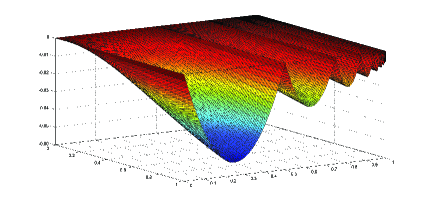
Figure 1. Continuous function $T$ of unbounded variation with generating function $\phi(x,y)=x(x-0.5)\sin y$.

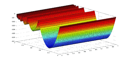
Figure 2. Continuous function $T$ of unbounded variation with generating function $\phi(x,y)=\sin\big{(}x(x-0.5)\big{)}$

Next we present a simple example of a function which is neither continuous nor of bounded variation, with its graph having the box dimension and Hausdorff dimension $2.$

Example 4.6.

Let $A=[a,b]\times[c,d]$ and define a function $f:A\rightarrow\mathbb{R}$ as follows.

$$f(x,y)=\begin{cases}0\quad\text{if}\quad x,y~{}~{}\text{are rational~{} numbers,}\\ 1\quad\text{otherwise}.\end{cases}$$

We may write the graph of the function $f$ as

$$\begin{split}G(f)=&~{}\big{\{}(x,y,0):(x,y)\in A\cap(\mathbb{Q}\times\mathbb{Q})\big{\}}\cup\big{\{}(x,y,1):(x,y)\in A\cap(\mathbb{Q}\times\mathbb{Q})^{c}\big{\}}\\ :=&~{}G_{1}\cup G_{2}\end{split}$$

The set $G_{1}$ is countable, so the Hausdorff measure is zero [3]. Using the countable additive property of Hausdorff measure [3], we have

$$\dim_{H}(G(f))=2.$$

Therefore $2=\dim_{H}(G(f))\leq\underline{\dim}_{B}(G(f))\leq\overline{\dim}_{B}(G(f)).$ Using a property of the upper box dimension [3], we have

$$\overline{\dim}_{B}(G_{1})=\overline{\dim}_{B}(\overline{G_{1}})=2,\quad\overline{\dim}_{B}(G_{2})=\overline{\dim}_{B}(\overline{G_{2}})=2.$$

Since $\overline{\dim}_{B}$ is finitely stable, we get

$$\overline{\dim}_{B}(G(f))=2.$$

Therefore, $\dim_{B}(G(f))=\dim_{H}(G(f))=2.$

Acknowledgements

The first author thanks the University Grants Commission (UGC), India for financial support in the form of a Senior Research Fellowship.

References

- [1] C. R. Adams, J. A. Clarkson, Properties of functions of bounded variation, Trans. Amer. Math. Soc., 36 (1934) 711-730.
- [2] J. A. Clarkson, C. R. Adams, On definitions of bounded variation for functions of two variables, Trans. Amer. Math. Soc., 35 (1933) 824-854.
- [3] K. J. Falconer, Fractal Geometry: Mathematical Foundations and Applications, John Wiley Sons Inc., New York, 1999.
- [4] U. N. Katugampola, New approach to a generalized fractional integral, Appl. Math. Comput., 218 (2011) 860-865.
- [5] A. A. Kilbas, H. M. Srivastava, J. J. Trujillo, Theory and applications of fractional differential equations, North-Holland Mathematics Studies, 204, Elsevier Science B.V., Amsterdam, 2006.
- [6] Y. S. Liang, Box dimensions of Riemann-Liouville fractional integrals of continuous functions of bounded variation, Nonlin. Anal., 72 (2010) 4304-4306.
- [7] Y. S. Liang, W.Y. Su, Fractal dimensions of fractional integral of continuous functions, Acta Math. Sin. (Engl. Ser.), 32(12) (2016) 1494-1508.
- [8] K. Yao, Y.S. Liang, F. Zhang, On the connection between the order of the fractional derivative and the Hausdorff dimension of a fractal function, Chaos, Solitons & Fractals, 41(5) (2009) 2538-2545.
- [9] E. C. Oliveira, J. A. Machado, A Review of definitions for fractional derivatives and integral, Math. Problems in Eng., 2014 (2014) Article ID 238459, 6 pages.
- [10] H-J Ruan, W-Y Su, K. Yao, Box dimension and fractional integral of linear fractal interpolation functions, J. Approx. Theory, 161(1) (2009) 187-197.
- [11] S. G. Samko, A. A. Kilbas, O. N. Marichev, Fractional Integrals and Derivatives: Theory and Applications, Gordon and Breach Science Publishers, 1993.
- [12] S. Verma, Some Results on Fractal Functions, Fractal Dimensions and Fractional Calculus, Ph.D. thesis, Indian Institute of Technology Delhi, India, 2020.
- [13] S. Verma, P. Viswanathan, A note on Katugampola fractional calculus and fractal dimensions, Appl. Math. Comp., 339 (2018) 220-230.
- [14] S. Verma, P. Viswanathan, Bivariate functions of bounded variation: Fractal dimension and fractional integral, Indag. Math., 31 (2020) 294-309.
- [15] W.X. Zheng, S.W. Wang, Real Function and Functional Analysis, High Education Publication, Beijing, 1980 (in Chinese).