Stochastic Learning Approach to Binary Optimization for Optimal Design of Experiments

Abstract

We present a novel stochastic approach to binary optimization for optimal experimental design (OED) for Bayesian inverse problems governed by mathematical models such as partial differential equations. The OED utility function, namely, the regularized optimality criterion, is cast into a stochastic objective function in the form of an expectation over a multivariate Bernoulli distribution. The probabilistic objective is then solved by using a stochastic optimization routine to find an optimal observational policy. The proposed approach is analyzed from an optimization perspective and also from a machine learning perspective with correspondence to policy gradient reinforcement learning. The approach is demonstrated numerically by using an idealized two-dimensional Bayesian linear inverse problem, and validated by extensive numerical experiments carried out for sensor placement in a parameter identification setup.

62K05, 35Q62, 62F15, 35R30, 35Q93, 65C60, 93E35

1 Introduction

Optimal experimental design (OED) is the general mathematical formalism for configuring an observational setup. This can refer to the frequency of data collection or the spatiotemporal distribution of observational gridpoints for physical experiments. OED has seen a recent surge of interest in the field sensor placement for applications of model-constrained Bayesian inverse problems; see, for example, [40, 22, 38, 50, 24, 26, 25, 28, 16, 2, 5, 4, 3, 1, 8, 9].

Many physical phenomena can be simulated by using mathematical models. The accuracy of the mathematical models is limited, however, by the level at which the physics of the true system is captured by the model and by the numerical errors produced, for example, by computer simulations. Model-based simulations are often corrected based on snapshots of reality, such as sensor-based measurements. Such corrections involve first inferring the model parameter from the noisy measurements, a problem referred to as the “inverse problem,” which can be solved by different inversion or data assimilation methods; see e.g.,  [13, 19, 35, 11, 10]. These observations themselves are noisy but in general follow a known probability distribution. The OED problem is concerned with finding the most informative, and thus optimal, observational grid configuration out of a set of candidates, which, when deployed, will result in a reliable solution of the inverse problem.

OED is most beneficial when there is a limit on the number of sensors that can be used, for example, when sensors are expensive to deploy and/or operate. In order to solve an OED problem for sensor placement, a binary optimization problem is formulated by assigning a binary design variable $\mathbf{{\zeta}}_{i}$ for each candidate sensor location. The objective is often set to a utility function that summarizes the uncertainty in the inversion parameter or the amount of information gained from the observations. The optimal design is then defined as the optimizer of this objective function. The objective is constrained by the model evolution equations, such as partial differential equations, and also by any regularity or sparsity constraints on the design. Here we focus on sparse and binary designs. A popular choice of a penalty function to enforce a sparse and binary design is the $\ell_{0}$ penalty [3].

Solving such binary optimization problems is computationally prohibitive, and often the binary optimization problem is replaced with a relaxation. In the relaxation of an OED problem, the design variable is allowed to take any value in the interval $[0,1]$ and is often interpreted as an importance weight of the candidate location. Once a solution of the relaxed problem is obtained numerically, for example, by a gradient-based optimization procedure, a binarization (rounding) procedure is required to transform the solution of the relaxed problem into an equivalent solution of the original problem. In general, however, the numerical solutions of the two problems are not guaranteed to be related or even similar.

Using a gradient-based approach to solve the relaxed OED problem requires many evaluations of the simulation model in order to evaluate the objective function and its gradient. Moreover, this approach requires the penalty function to be differentiable with respect to the design variables. To this end, since $\ell_{0}$ is discontinuous, numerous efforts have been dedicated to approximating the effect of $\ell_{0}$ sparsification with other approaches. For example, in [24], an $\ell_{1}$ penalty followed by a thresholding method is used; however, $\ell_{1}$ is nonsmooth and hence is nondifferentiable. Continuation procedures are used in [3, 32], where a series of OED problems are solved with a sequence of penalty functions that successively approximate $\ell_{0}$ sparsification. Another approach that can potentially induce a binary design is the sum-up-rounding algorithm [53], which also provides optimality guarantees.

Here we propose a new efficient approach for directly solving the original binary OED problem. In this framework, the objective function, namely, the regularized optimality criterion, is cast into an objective function in the form of an expectation over a multivariate Bernoulli distribution. A stochastic optimization approach is then applied to solve the reformulated optimization problem in order to find an optimal observational policy.

Related work on stochastic optimization for OED has been explored in [27], where the utility function, in other words, the optimality criterion, is approximated by using Monte Carlo estimators. A stochastic optimization procedure is then applied with the gradient of the utility function with respect to the design being approximated by using Robbins–Monro stochastic approximation [42], or sample average approximation [47, 36].

The main differences from the standard OED approach and previous stochastic OED approaches, which highlight our main contributions in this work, are as follows. First, the proposed methodology searches for an optimal probability distribution representing the optimal binary design; hence it does not require relaxation or binarization to follow the optimization step as in the traditional OED formulation. Second, in our approach the penalized OED criterion is not required to be differentiable with respect to the design. Thus, one can incorporate the $\ell_{0}$ regularization norm to enforce sparsification without needing to approximate it with the $\ell_{1}$ penalty term or apply a continuation procedure to retrieve a binary optimal design. Third, the proposed stochastic OED formulation does not require formulating the gradient of the objective function with respect to the design, thus implying a massive reduction in computation cost. Fourth, the proposed approach and solution algorithms are completely independent from the specific choice of the OED optimality criterion and the penalty function and hence can be used with both linear and nonlinear problems.

In this work, for simplicity we provide numerical experiments for Bayesian inverse problems constrained by linear forward operators, and we consider an A-optimal design, that is, a design that minimizes the trace of the posterior covariances of the inversion parameter. The approach proposed, however, extends easily to other OED optimality criteria, such as D-optimality. We provide an analysis of the method from a mathematical point of view and an interpretation from a machine learning (ML) perspective. Specifically, the proposed algorithm has a direct link to policy gradient algorithms widely used in neuro-dynamic programming and reinforcement learning [14, 51, 49]. Numerical experiments using a toy example are provided to help with understanding the problem; the proposed algorithm; and the relation between the binary OED problem, the relaxed OED problem, and the proposed formulation. Moreover, extensive numerical experiments are performed for optimal sensor placement for an advection-diffusion problem that simulates the spatiotemporal evolution of the concentration of a contaminant in a bounded domain.

The paper is organized as follows. Section 2 gives a brief description of the Bayesian inverse problem and the standard formulation of an optimal experimental design in the context of Bayesian inversion. In Section 3, we describe our proposed approach for solving the binary OED problem and present a detailed analysis of the proposed algorithms. An explanatory example and extensive numerical experiments are given in Section 4. Discussion and concluding remarks are presented in Section 5.

Throughout the paper, we use boldface symbols for vectors and matrices. $\mathsf{diag}\left(\mathbf{{x}}\right)$ is a diagonal matrix with diagonal entries set to the entries of the vector $\mathbf{{x}}$. The $i$th cardinality vector in the Euclidean space $\mathbb{R}^{n}$ is denoted by $\mathbf{{e}}_{i}\in\mathbb{R}^{n}$. Subscripts refer to entries of vectors and matrices, and square brackets are used to symbolize instances of a vector, for example, randomly drawn from a particular distribution. Superscripts with round brackets are reserved for iterations in optimization routines.

2 OED for Bayesian Inversion

Consider the forward model described by

(1) $$\mathbf{y}=\mathbf{F}(\mathbf{{\theta}})+\mathbf{{\delta}}\,,$$

where $\mathbf{{\theta}}\in\mathbb{R}^{\textsc{N}_{\rm state}}$ is the discretized model parameter and $\mathbf{y}\in\mathbb{R}^{\textsc{N}_{\rm obs}}$ is the observation, where $\mathbf{{\delta}}\in\mathbb{R}^{\textsc{N}_{\rm obs}}$ is the observation error. Assuming Gaussian observational noise $\mathbf{{\delta}}\sim\mathcal{N}\!\left({\mathbf{{0}}},{\mathbf{{\Gamma}}_{{\rm noise}}}\right)$, then the data likelihood takes the form

(2) $$\mathcal{L}{\left(\mathbf{y}|\mathbf{{\theta}}\right)}\propto\exp{\left(-\frac{1}{2}\left\|{\mathbf{F}(\mathbf{{\theta}})-\mathbf{y}}\right\|^{2}_{\mathbf{{\Gamma}}_{{\rm noise}}^{-1}}\right)}\,,$$

where $\mathbf{{\Gamma}}_{{\rm noise}}$ is the observation error covariance matrix (positive definite) and the matrix-weighted norm is defined as $\left\|{\mathbf{{x}}}\right\|^{2}_{\mathbf{{A}}}=\mathbf{{x}}^{\mkern-1.5mu\mathsf{T}}\mathbf{{A}}\mathbf{{x}}$.

An inverse problem refers to the retrieval of the model parameter $\mathbf{{\theta}}$ from the noisy observation $\mathbf{y}$, conditioned by the model dynamics. In Bayesian inversion, the goal is to study the probability distribution of $\mathbf{{\theta}}$ conditioned by the observation $\mathbf{y}$ that is the posterior obtained by applying Bayes’ theorem,

(3) $$\mathbb{P}\left(\mathbf{{\theta}}|\mathbf{y}\right)\propto\mathbb{P}\left(\mathbf{y}|\mathbf{{\theta}}\right)\mathbb{P}(\mathbf{{\theta}})\,$$

where $\mathbb{P}(\mathbf{{\theta}})$ is the prior distribution of the inversion parameter $\mathbf{{\theta}}$, which in many cases is assumed to be Gaussian $\mathbf{{\theta}}\sim\mathcal{N}\!\left({\mathbf{{\theta}}_{\rm pr}},{\mathbf{{\Gamma}}_{{\rm pr}}}\right)$. If the parameter-to-observable map $\mathbf{F}$ is linear, the posterior $\mathbb{P}\left(\mathbf{{\theta}}|\mathbf{y}\right)$ is Gaussian $\mathcal{N}\!\left({\mathbf{{\theta}}_{\rm post}^{\mathbf{y}}},{\mathbf{{\Gamma}}_{{\rm post}}}\right)$ with

(4) $$\mathbf{{\Gamma}}_{{\rm post}}=\left(\mathbf{F}^{\mkern-1.5mu\mathsf{*}}\mathbf{{\Gamma}}_{{\rm noise}}^{-1}\mathbf{F}+\mathbf{{\Gamma}}_{{\rm pr}}^{-1}\right)^{-1}\,,\quad\mathbf{{\theta}}_{\rm post}^{\mathbf{y}}=\mathbf{{\Gamma}}_{{\rm post}}\left(\mathbf{{\Gamma}}_{{\rm pr}}^{-1}\mathbf{{\theta}}_{\rm pr}+\mathbf{F}^{\mkern-1.5mu\mathsf{*}}\mathbf{{\Gamma}}_{{\rm noise}}^{-1}\,\mathbf{y}\right)\,,$$

where $\mathbf{F}^{\mkern-1.5mu\mathsf{*}}$ is the forward operator adjoint. If the forward operator $\mathbf{F}$ is nonlinear, however, the posterior distribution is no longer Gaussian. A Gaussian approximation of the posterior can be obtained in this case by linearization of $\mathbf{F}$ around the maximum a posteriori (MAP) estimate, which is inherently data dependent. For simplicity, we will focus on linear models; however, the approach proposed in this work is not limited to the linear case. Further analysis for nonlinear settings will follow in separate works.

In a Bayesian OED context (see, e.g., [1, 2, 3, 8, 9, 24, 25]), the observation covariance $\mathbf{{\Gamma}}_{{\rm noise}}$ is replaced with a weighted version $\mathbf{{W}}_{\Gamma}(\mathbf{{\zeta}})$, parameterized by the design $\mathbf{{\zeta}}$, resulting in the following weighted data-likelihood $\mathcal{L}{\left(\mathbf{y}|\mathbf{{\theta}};\mathbf{{\zeta}}\right)}$ and posterior covariance $\mathbf{{\Gamma}}_{{\rm post}}(\mathbf{{\zeta}})$.

(5) $$\mathcal{L}{\left(\mathbf{y}|\mathbf{{\theta}};\mathbf{{\zeta}}\right)}\propto\exp{\left(-\frac{1}{2}\left\|{\mathbf{F}(\mathbf{{\theta}})-\mathbf{y}}\right\|^{2}_{\mathbf{{W}}_{\Gamma}(\mathbf{{\zeta}})}\right)}\,,\quad\mathbf{{\Gamma}}_{{\rm post}}(\mathbf{{\zeta}})=\left(\mathbf{F}^{\mkern-1.5mu\mathsf{*}}\mathbf{{W}}_{\Gamma}(\mathbf{{\zeta}})\mathbf{F}+\mathbf{{\Gamma}}_{{\rm pr}}^{-1}\right)^{\mkern-1.5mu\mathsf{-1}}\,.$$

The exact form of the posterior covariance $\mathbf{{\Gamma}}_{{\rm post}}(\mathbf{{\zeta}})$ depends on how $\mathbf{{W}}_{\Gamma}(\mathbf{{\zeta}})$ is formulated. We are interested mainly in binary designs $\mathbf{{\zeta}}\in\{0,1\}^{n_{\rm s}}$, required, for example, in sensor placement applications; see, for example, [1, 9]. In this case, we assume a set of $n_{\rm s}$ candidate sensor locations, and we seek the optimal subset of locations. Note that selecting a subset of the observations is equivalent to applying a projection operator onto the subspace spanned by the activated sensors. This is equivalent to defining the weighed design matrix as $\mathbf{{W}}_{\Gamma}:=\mathbf{{\Gamma}}_{{\rm noise}}^{-1/2}\mathbf{{W}}\mathbf{{\Gamma}}_{{\rm noise}}^{-1/2}$, where $\mathbf{{W}}:=\mathsf{diag}\left(\mathbf{{\zeta}}\right)$ is a diagonal matrix with binary values on its diagonal. The $i$th entry of the design is set to $1$ to activate a sensor and is set to $0$ to turn it off.

The optimal design $\mathbf{{\zeta}}^{\mkern-1.5mu\mathrm{opt}}$ is the one that optimizes a predefined criterion $\Psi(\cdot)$ of choice. The most popular optimality criteria in the Bayesian inversion context are A- and D-optimality. Both criteria define the optimal design as the one that minimizes a scalar summary of posterior uncertainty associated with an inversion parameter or state of an inverse problem. Specifically, $\Psi(\mathbf{{\zeta}}):=\mathrm{Tr}\left(\mathbf{{\Gamma}}_{{\rm post}}(\mathbf{{\zeta}})\right)$ for an A-optimal design, and $\Psi(\mathbf{{\zeta}}):=\log\det\left(\mathbf{{\Gamma}}_{{\rm post}}(\mathbf{{\zeta}})\right)$ for a D-optimal design, i.e., the sum of the eigenvalues of $\mathbf{{\Gamma}}_{{\rm post}}(\mathbf{{\zeta}})$, and the sum of the logarithms of the eigenvalues of $\mathbf{{\Gamma}}_{{\rm post}}(\mathbf{{\zeta}})$, respectively.

To prevent experimental designs that are simply dense, one typically adds a regularization term $\Phi(\mathbf{{\zeta}})$ that promotes sparsity, for example. Thus, to find an optimal design $\mathbf{{\zeta}}^{\mkern-1.5mu\mathrm{opt}}$, one needs to solve the following binary optimization problem,

(6) $$\mathbf{{\zeta}}^{\mkern-1.5mu\mathrm{opt}}=\operatorname*{arg\,min}_{\mathbf{{\zeta}}\in\{0,1\}^{n_{\rm s}}}\mathcal{J}(\mathbf{{\zeta}}):=\Psi(\mathbf{{\zeta}})\,+\alpha\,\Phi(\mathbf{{\zeta}})\,,$$

where the function $\Phi(\mathbf{{\zeta}})$ promotes regularization or sparsity on the design and $\alpha$ is a user-defined regularization parameter. For example, $\Phi$ could represent a budget constraint on the form $\Phi(\mathbf{{\zeta}}):=\left\|{\mathbf{{\zeta}}}\right\|_{0}\leq k\,;k\in\mathtt{Z}_{+}$ or a sparsifying (possibly discontinuous) function, for example, $\left\|{\mathbf{{\zeta}}}\right\|_{0}$ or $\left\|{\mathbf{{\zeta}}}\right\|_{1}$.

Traditional binary optimization approaches [52] for solving the optimization problem are expensive, rendering the exact solution of (6) computationally intractable. The optimization problem (7) is a continuous relaxation of (6) and is often used in practice as a surrogate for solving (6) with a suitable rounding scheme:

(7) $$\mathbf{{\zeta}}^{\mkern-1.5mu\mathrm{opt}}=\operatorname*{arg\,min}_{\mathbf{{\zeta}}\in[0,1]^{n_{\rm s}}}\mathcal{J}(\mathbf{{\zeta}}):=\Psi(\mathbf{{\zeta}})\,+\alpha\,\Phi(\mathbf{{\zeta}})\,.$$

In sensor placement we seek a sparse design in order to minimize the deployment cost, and thus we would utilize $\ell_{0}$ as a penalty function. Solving the relaxed optimization problem (7) follows a gradient-based approach, and thus using $\ell_{0}$ as a penalty function is replaced with the nonsmooth $\ell_{1}$ norm; see [3] for more details.

The relaxed problem (7) provides a lower bound on (6), and any binary solution $\mathbf{{\zeta}}^{\mkern-1.5mu\mathrm{opt}}\in\{0,1\}^{n}_{\rm s}$ of (7) is also an optimal solution of (6). Given a solution of (7) that is not binary, we can obtain a binary solution by rounding; however, there is no guarantee that the resulting binary solution is optimal, unless we use sum-up-rounding. In Section 3 we present a new approach for directly solving the original OED binary optimization problem (6) without the need to relax the design space or to round the relaxations.

3 Stochastic Learning Approach for Binary OED

Our main goal is to find the solution of the original binary regularized OED problem (6) without solving a mixed-integer programming problem or resorting to the relaxation approach widely followed in OED for Bayesian inversion (as summarized in Section 2). We propose to reformulate and solve the binary optimization problem (6) as a stochastic optimization problem defined over the parameters of a probability distribution. Specifically, we assume $\mathbf{{\zeta}}$ is a random variable that follows a multivariate Bernoulli distribution.

3.1 Stochastic formulation of the OED problem

We associate with each candidate sensor location $x_{i}$ a probability of activation $\mathbf{{\theta}}_{i}$. Specifically, we assume that $\mathbf{{\zeta}}_{i},\,i=1,2,\ldots,n_{\rm s}$ are independent Bernoulli random variables associated with the candidate sensor locations $x_{i},\,i=1,2,\ldots,n_{\rm s}$. The activation (success) probabilities of the respective sensors are $\mathbf{{\theta}}_{i},\,i=1,2,\ldots,n_{\rm s}$; that is, $\mathbb{P}(\mathbf{{\zeta}}_{i}=1)=\mathbf{{\theta}}_{i},\,\mathbb{P}(\mathbf{{\zeta}}_{i}=0)=1-\mathbf{{\theta}}_{i}$. The probability associated with any observational configuration is then described by the joint probability of all candidate locations. Note that assuming independent activation variables $\mathbf{{\zeta}}_{i}$ does not interfere the correlation structure of the observational errors, manifested by the observation error covariance matrix $\mathbf{{\Gamma}}_{{\rm noise}}$. Conversely, setting $\mathbf{{\zeta}}_{i}$ to $0$ corresponds to removing the $i$th row and column from the precision matrix $\mathbf{{\Gamma}}_{{\rm noise}}^{\mkern-1.5mu\mathsf{-1}}$, while setting the design variable value to $1$ corresponds to keeping the corresponding row and column, respectively. We let $\mathbb{P}\left(\mathbf{{\zeta}}|\mathbf{{\theta}}\right)$ denote the joint multivariate Bernoulli probability, with the following probability mass function (PMF):

(8) $$\mathbb{P}\left(\mathbf{{\zeta}}|\mathbf{{\theta}}\right):=\prod_{i=1}^{n_{\rm s}}{\mathbf{{\theta}}_{i}^{\mathbf{{\zeta}}_{i}}\,\left(1-\mathbf{{\theta}}_{i}\right)^{1-\mathbf{{\zeta}}_{i}}}\,,\quad\mathbf{{\zeta}}_{i}\in\{0,1\},\,\quad\mathbf{{\theta}}_{i}\in[0,1]\,.$$

We then replace the original problem (6) with the following stochastic optimization problem:

(9) $$\mathbf{{\theta}}^{\mkern-1.5mu\mathrm{opt}}=\operatorname*{arg\,min}_{\mathbf{{\theta}}\in[0,1]^{n_{\rm s}}}\Upsilon(\mathbf{{\theta}}):=\mathbb{E}_{\mathbf{{\zeta}}\sim\mathbb{P}\left(\mathbf{{\zeta}}|\mathbf{{\theta}}\right)}{\Bigl{[}\mathcal{J}(\mathbf{{\zeta}})\Bigr{]}}=\mathbb{E}_{\mathbf{{\zeta}}\sim\mathbb{P}\left(\mathbf{{\zeta}}|\mathbf{{\theta}}\right)}{\Bigl{[}\Psi(\mathbf{{\zeta}})+\alpha\,\Phi(\mathbf{{\zeta}})\Bigr{]}}\,.$$

Because the support of the probability distribution is discrete, the possible values of $\mathbf{{\zeta}}\in\{0,1\}^{n_{\rm s}}$ are countable and can be assigned unique indexes. An index $k$ is assigned to each possible realization of $\mathbf{{\zeta}}:=(\mathbf{{\zeta}}_{1},\mathbf{{\zeta}}_{2},\ldots,\mathbf{{\zeta}}_{n_{\rm s}})$, based on the values of its components using the relation

(10) $$k=1+\sum_{i=1}^{n_{\rm s}}{\mathbf{{\zeta}}_{i}\,2^{i-1}}\,,\quad\mathbf{{\zeta}}_{i}\in\{0,1\}\,.$$

Thus, all possible designs are labeled as $\mathbf{{\zeta}}[k],k\!=\!1,2,\ldots,2^{n_{\rm s}}$. With the indexing scheme (10), the optimization problem (9) takes the following equivalent form:

(11) $$\mathbf{{\theta}}^{\mkern-1.5mu\mathrm{opt}}=\operatorname*{arg\,min}_{\mathbf{{\theta}}\in[0,1]^{n_{\rm s}}}\Upsilon(\mathbf{{\theta}}):=\sum_{k=1}^{2^{n_{\rm s}}}\mathcal{J}(\mathbf{{\zeta}}[k])\mathbb{P}\left(\mathbf{{\zeta}}[k]|\mathbf{{\theta}}\right)\,.$$

To solve (11), one can follow a gradient-based optimization approach to find the optimal parameter $\mathbf{{\theta}}^{\mkern-1.5mu\mathrm{opt}}$. The gradient of the objective in (11) with respect to the distribution parameters $\mathbf{{\theta}}$ is

(12) $$\nabla_{\mathbf{{\theta}}}\,\Upsilon(\mathbf{{\theta}})=\nabla_{\mathbf{{\theta}}}\,\mathbb{E}_{\mathbf{{\zeta}}\sim\mathbb{P}\left(\mathbf{{\zeta}}|\mathbf{{\theta}}\right)}{\Bigl{[}\mathcal{J}(\mathbf{{\zeta}})\Bigr{]}}=\nabla_{\mathbf{{\theta}}}\,\sum_{\mathbf{{\zeta}}}\mathcal{J}(\mathbf{{\zeta}})\mathbb{P}\left(\mathbf{{\zeta}}|\mathbf{{\theta}}\right)=\sum_{k=1}^{2^{n_{\rm s}}}\mathcal{J}(\mathbf{{\zeta}}[k])\nabla_{\mathbf{{\theta}}}\,\mathbb{P}\left(\mathbf{{\zeta}}[k]|\mathbf{{\theta}}\right)\,,$$

where $\nabla_{\mathbf{{\theta}}}\,\mathbb{P}\left(\mathbf{{\zeta}}|\mathbf{{\theta}}\right)$ is the gradient of the joint Bernoulli PMF (8) (see Appendix A for details):

(13) $$\nabla_{\mathbf{{\theta}}}\,\mathbb{P}\left(\mathbf{{\zeta}}[k]|\mathbf{{\theta}}\right)=\sum_{j=1}^{n_{\rm s}}\left.\frac{\partial{\mathbb{P}\left(\mathbf{{\zeta}}[k]|\mathbf{{\theta}}\right)}}{\partial{\mathbf{{\theta}}_{j}}}\right|_{\mathbf{{\zeta}}=\mathbf{{\zeta}}[k]}=\sum_{j=1}^{n_{\rm s}}(-1)^{1-\mathbf{{\zeta}}_{j}[k]}\prod_{\begin{subarray}{c}i=1\\ i\neq j\end{subarray}}^{n_{\rm s}}{\mathbf{{\theta}}_{i}^{\mathbf{{\zeta}}_{i}[k]}\left(1-\mathbf{{\theta}}_{i}\right)^{1-\mathbf{{\zeta}}_{i}[k]}}\mathbf{{e}}_{j}\,.$$

In Appendix A, we provide a detailed discussion of the multivariate Bernoulli distribution, with identities and lemmas that will be useful for the following discussion.

Clearly, (11) and (12) are not practical formula, because their statement alone requires the evaluation of all possible designs $\mathcal{J}(\mathbf{{\zeta}}[k])$, which is equivalent to complete enumeration of (6). We show below how we can utilize stochastic gradient approaches to avoid complete enumeration. Practical and efficient solution of (9) is discussed in Section 3.3. We first establish in Section 3.2 the connection between the solution of the two problems (6) and (9) and discuss the benefits of the proposed approach.

3.2 Benefits of the stochastic formulation

The connections between the two problems (6 and 9) and their respective solutions are summarized by Proposition 3.1 and Lemma 3.3. The relation between the objective functions in these two problems, and their domains and codomains, is sketched in Figure 1.

Proposition 3.1.

Consider the two functions $\mathcal{J}:\Omega_{\mathbf{{\zeta}}}:=\{0,1\}^{n_{\rm s}}\to\mathbb{R}$ and $\Upsilon:\Omega_{\mathbf{{\theta}}}:=[0,1]^{n_{\rm s}}\to\mathbb{R}$, defined in (6) and (9), respectively. Let $\mathbf{{\zeta}}\in\Omega_{\mathbf{{\zeta}}}$ be a random vector following the multivariate Bernoulli distribution (8), with parameter $\mathbf{{\theta}}\in\Omega_{\mathbf{{\theta}}}$. Let $C:=\{c\!\in\!\mathbb{R}\,|\,c\!:=\!\mathcal{J}(\mathbf{{\zeta}})\,,\,\mathbf{{\zeta}}\in\Omega_{\mathbf{{\zeta}}}\}$, be the set of objective values corresponding to all possible designs, $\mathbf{{\zeta}}\in\Omega_{\mathbf{{\zeta}}}$. Then:

1. $\Omega_{\mathbf{{\theta}}}$ is the convex hull of $\Omega_{\mathbf{{\zeta}}}$ in $\mathbb{R}^{n_{\rm s}}$.

2. The values of $\Upsilon$ (9) form the convex hull of $C$ in $\mathbb{R}$, denoted by $conv(C)$, with points $c\in C$ being the extreme points of $conv(C)$; that is, $conv(C)\equiv\{\Upsilon(\mathbf{{\theta}})|\mathbf{{\theta}}\in\Omega_{\mathbf{{\theta}}}\}$.

3. $\Upsilon(\mathbf{{x}})=\mathcal{J}(\mathbf{{x}})\,\forall\mathbf{{x}}\in{\Omega_{\mathbf{{\zeta}}}}$.

4. For any realization of $\mathbf{{\theta}}\in\Omega_{\mathbf{{\theta}}}$, it holds that $\min\{C\}\leq\Upsilon(\mathbf{{\theta}})\leq\max\{C\}$; moreover, $\Upsilon(\mathbf{{\theta}}^{\mkern-1.5mu\mathrm{opt}})=\min\{C\}=\mathcal{J}(\mathbf{{\zeta}}^{\mkern-1.5mu\mathrm{opt}})$.

Proof 3.2.

1. This follows from the definition of $\Omega_{\mathbf{{\zeta}}}$ and $\Omega_{\mathbf{{\theta}}}$ and the fact that $\Omega_{\mathbf{{\theta}}}$ is the hypercube in $\mathbb{R}^{n_{\rm s}}$ whose vertices formulate the set $\Omega_{\mathbf{{\zeta}}}$.

2. For any realization $\mathbf{{\theta}}$, the function $\Upsilon$ defines a convex combination of all points in $C$, because the coefficients $\mathbb{P}\left(\mathbf{{\zeta}}|\mathbf{{\theta}}\right),\,\mathbf{{\zeta}}\in\Omega_{\mathbf{{\zeta}}}$ are probabilities satisfying that $0\leq\mathbb{P}\left(\mathbf{{\zeta}}|\mathbf{{\theta}}\right)\leq 1$ and $\sum_{\mathbf{{\zeta}}\in\Omega_{\mathbf{{\zeta}}}}\mathbb{P}\left(\mathbf{{\zeta}}|\mathbf{{\theta}}\right)=1$.

3. Setting $\mathbf{{\theta}}$ to any $\mathbf{{x}}\in\Omega_{\mathbf{{\zeta}}}$ yields a degenerate multivariate Bernoulli distribution, which is a Dirac measure $\delta_{\mathbf{{\zeta}}}(\{\mathbf{{x}}\})$ defined on the set $\{\mathbf{{x}}\}$. Thus, $\mathbb{P}\left(\mathbf{{\zeta}}|\mathbf{{\theta}}=\mathbf{{x}}\right)=\delta_{\mathbf{{\zeta}}}(\{\mathbf{{x}}\})$, and $\Upsilon(\mathbf{{x}})=\sum_{\mathbf{{\zeta}}\in\Omega_{\mathbf{{\theta}}}}\mathbb{P}\left(\mathbf{{\zeta}}|\mathbf{{\theta}}\!=\!\mathbf{{x}}\right)\mathcal{J}(\mathbf{{\zeta}})=\sum_{\mathbf{{\zeta}}\in\Omega_{\mathbf{{\theta}}}}\delta_{\mathbf{{\zeta}}}(\{\mathbf{{x}}\})\,\mathcal{J}(\mathbf{{\zeta}})=\mathcal{J}(\mathbf{{x}})\,$.

4. It follows from Carathéodory’s theorem that for any realization of $\mathbf{{\theta}}\in\Omega_{\mathbf{{\theta}}}$, the value of the objective $\Upsilon(\mathbf{{\theta}})$ falls on a line segment in $\mathbb{R}$ that connects at most two points in $C$. This guarantees that $\min\{C\}\leq\Upsilon(\mathbf{{\theta}})\leq\max\{C\}$. Additionally, from points a) and b) above, it follows that $\Upsilon(\mathbf{{\theta}}^{\mkern-1.5mu\mathrm{opt}})=\min\{conv(C)\}=\min\{C\}=\mathcal{J}(\mathbf{{\zeta}}^{\mkern-1.5mu\mathrm{opt}})$.

Figure 1: Relation between problems 6 and 9 and their respective domains and codomains.

Lemma 3.3.

The optimal solutions of the two problems (6) and (9) are such that

$$\operatorname*{arg\,min}\limits_{\mathbf{{\zeta}}\in\Omega_{\mathbf{{\zeta}}}}{\mathcal{J}(\mathbf{{\zeta}})}\subseteq\operatorname*{arg\,min}\limits_{\mathbf{{\theta}}\in\Omega_{\mathbf{{\theta}}}}{\Upsilon(\mathbf{{\theta}})}\,.$$

Moreover, if the optimal solution $\mathbf{{\zeta}}^{\mkern-1.5mu\mathrm{opt}}$ of (6) is unique, then $\mathbf{{\theta}}^{\mkern-1.5mu\mathrm{opt}}=\mathbf{{\zeta}}^{\mkern-1.5mu\mathrm{opt}}$, where $\mathbf{{\theta}}^{\mkern-1.5mu\mathrm{opt}}$ is the unique optimal solution of (9).

Proof 3.4.

Proposition 3.1 guarantees that $\nexists\mathbf{{\theta}}\in\Omega_{\mathbf{{\theta}}},\,\Upsilon(\mathbf{{\theta}})<\mathcal{J}(\mathbf{{\zeta}}^{\mkern-1.5mu\mathrm{opt}})$. Additionally, from points a) and c) in Proposition 3.1, it follows that $\operatorname*{arg\,min}\limits_{\mathbf{{\zeta}}\in\Omega_{\mathbf{{\zeta}}}}{\mathcal{J}(\mathbf{{\zeta}})}\subseteq\operatorname*{arg\,min}\limits_{\mathbf{{\theta}}\in\Omega_{\mathbf{{\theta}}}}{\Upsilon(\mathbf{{\theta}})}\,$.

Assume $\mathbf{{\zeta}}^{\mkern-1.5mu\mathrm{opt}}$ is the unique optimal solution of (6); it follows that $\mathbf{{\theta}}^{\mkern-1.5mu\mathrm{opt}}=\mathbf{{\zeta}}^{\mkern-1.5mu\mathrm{opt}}$ is an optimal solution of (9). Now assume $\exists\mathbf{{\theta}}\in\Omega_{\mathbf{{\theta}}}$ such that $\mathbf{{\theta}}\neq\mathbf{{\theta}}^{\mkern-1.5mu\mathrm{opt}},\,\Upsilon(\mathbf{{\theta}})=\Upsilon(\mathbf{{\theta}}^{\mkern-1.5mu\mathrm{opt}})=\mathcal{J}(\mathbf{{\zeta}}^{\mkern-1.5mu\mathrm{opt}})$. If $\mathbf{{\theta}}$ is the parameter of a degenerate Bernoulli distribution, then $\mathbf{{\theta}}\in\Omega_{\mathbf{{\zeta}}}$ and $\mathcal{J}(\mathbf{{\theta}})=\mathcal{J}(\mathbf{{\zeta}}^{\mkern-1.5mu\mathrm{opt}})$, thus contradicting the uniqueness of $\mathbf{{\zeta}}^{\mkern-1.5mu\mathrm{opt}}$. Conversely, if $\mathbf{{\theta}}$ is the parameter of a nondegenerate multivariate Bernoulli distribution, then there are at least two designs $\mathbf{{\zeta}},\mathbf{{\eta}}\in\Omega_{\mathbf{{\zeta}}}$ with nontrivial probabilities $\in(0,1)$, with $\mathcal{J}(\mathbf{{\zeta}})=\mathbf{{\zeta}}(\mathbf{{\eta}})$, again contradicting the uniqueness assumption of $\mathbf{{\zeta}}^{\mkern-1.5mu\mathrm{opt}}$.

The stochastic formalism proposed in Section 3.1 is beneficial for multiple reasons. First, this probabilistic formulation (9) to solving the original optimization problem (6) enables converting a binary design domain into a bounded continuous domain, where the optimal solution of the two problems (9) and (6) coincide. Second, the stochastic formulation (9) enables utilizing efficient stochastic optimization algorithms to solve binary optimization problems, which are not applicable for the deterministic binary optimization problem (6). Third, the solution of the stochastic problem (9) is an optimal parameter $\mathbf{{\theta}}^{\mkern-1.5mu\mathrm{opt}}$ that can be used for sampling binary designs $\mathbf{{\zeta}}$ by sampling $\mathbb{P}\left(\mathbf{{\zeta}}|\mathbf{{\theta}}^{\mkern-1.5mu\mathrm{opt}}\right)$ , even if only a suboptimal solution is found. Fourth, the stochastic formulation (9) requires evaluating the derivative of $\Upsilon$ with respect to the parameter of the probability distribution $\mathbf{{\theta}}$, instead of the design $\mathbf{{\zeta}}$. Thus, we do not need to evaluate the derivative of $\mathcal{J}$ with respect to the design $\mathbf{{\zeta}}$. In OED for Bayesian inversion, as discussed in Section 2, evaluating the gradient (with respect to the design) is very expensive since it requires many forward and backward solves of expensive simulation models. Fifth, because $\mathcal{J}$ is not required to be differentiable with respect to the design $\mathbf{{\zeta}}$, a nonsmooth penalty function $\Phi$ can be utilized in defining $\mathcal{J}$, for example to enforce sparsity or budget constraints, with the need to approximate this penalty with a smoother penalty approximation. Note that in this case, as explained by (6 and 9), the penalty is asserted on the design, rather than the distribution parameter $\mathbf{{\theta}}$.

3.3 Approximately solving the stochastic OED optimization problem

The objective in (11) and the gradient (12) amount to evaluating a large finite sum, which can be approximated by sampling. The simplest approach for approximately solving  (11) is to follow a Monte Carlo (MC) sample-based approximation to the objective $\Upsilon$ and the gradient $\nabla_{\mathbf{{\theta}}}\Upsilon$, where the sample is drawn from an appropriate probability distribution. However, the objective (9) is deterministic with respect to $\mathbf{{\theta}}$. Nevertheless, one can add randomness by assuming a uniform random variable (an index) over all terms of the objective and the associated gradient. This allows utilizing external and internal sampling-based stochastic optimization algorithms; see, for example, [34, 31, 21, 30, 46, 20, 41, 45]. These algorithms, however, are beyond the scope of this work.

Here, instead, we focus on efficient algorithmic procedures inspired by recent developments in reinforcement learning [14, 51, 49]. Specifically, we view $\mathbb{P}\left(\mathbf{{\zeta}}|\mathbf{{\theta}}\right)$ as a policy and the design $\mathbf{{\zeta}}$ as a state, and we seek an optimal policy to configure the observational grid. The reward is prescribed by the value of the original objective function, and we seek the optimal design that minimizes the total expected reward. This is further explained below.

An alternative form of the gradient (12) can be obtained by using the “kernel trick”, which utilizes the fact that $\nabla_{\mathbf{{\theta}}}{\log(\mathbb{P}\left(\mathbf{{\zeta}}|\mathbf{{\theta}}\right))}=\frac{1}{\mathbb{P}\left(\mathbf{{\zeta}}|\mathbf{{\theta}}\right)}\nabla_{\mathbf{{\theta}}}{\mathbb{P}\left(\mathbf{{\zeta}}|\mathbf{{\theta}}\right)}$, and thus $\nabla_{\mathbf{{\theta}}}{\mathbb{P}\left(\mathbf{{\zeta}}|\mathbf{{\theta}}\right)}={\mathbb{P}\left(\mathbf{{\zeta}}|\mathbf{{\theta}}\right)}\,\nabla_{\mathbf{{\theta}}}{\log(\mathbb{P}\left(\mathbf{{\zeta}}|\mathbf{{\theta}}\right))}$. Using this identity, we can rewrite the gradient (12) as

(14) $$\nabla_{\mathbf{{\theta}}}\,\Upsilon(\mathbf{{\theta}})=\sum_{k=1}^{2^{n_{\rm s}}}\Bigl{(}\mathcal{J}(\mathbf{{\zeta}}[k])\,\nabla_{\mathbf{{\theta}}}\,\log{\mathbb{P}\left(\mathbf{{\zeta}}[k]|\mathbf{{\theta}}\right)}\Bigr{)}\mathbb{P}\left(\mathbf{{\zeta}}[k]|\mathbf{{\theta}}\right)=\mathbb{E}_{\mathbf{{\zeta}}\sim\mathbb{P}\left(\mathbf{{\zeta}}|\mathbf{{\theta}}\right)}{\Bigl{[}\mathcal{J}(\mathbf{{\zeta}})\,\nabla_{\mathbf{{\theta}}}\,\log{\mathbb{P}\left(\mathbf{{\zeta}}|\mathbf{{\theta}}\right)}\Bigr{]}}\,.$$

We assume, without loss of generality, that $\mathbf{{\theta}}$ falls inside the open ball $(0,1)^{n_{\rm s}}$, and thus both the logarithm and the associated derivative of the log-probability are well defined. If any of the components of $\mathbf{{\theta}}$ attain their bound, then the distribution becomes degenerate in this direction, and the probability is set to either $0$ or $1$ and is thus taken out of the formulation since the gradient in that direction is set to $0$. This is equivalent to projecting $\mathbf{{\theta}}$ onto a lower-dimensional subspace.

The form of the gradient described by (14) is equivalent to (12). However, it shows that the gradient can be written as an expectation of gradients. This enables us to approximate the gradient using MC sampling by following a stochastic optimization approach. Specifically. given a sample $\mathbf{{\zeta}}[j]\sim\mathbb{P}\left(\mathbf{{\zeta}}|\mathbf{{\theta}}\right),\,j=1,2,\ldots,\textsc{N}_{\rm ens}$, we can use the following MC approximation of the gradient,

(15) $$\mathbf{{g}}:=\nabla_{\mathbf{{\theta}}}\,\mathbb{E}_{\mathbb{P}\left(\mathbf{{\zeta}}|\mathbf{{\theta}}\right)}{\Bigl{[}\mathcal{J}(\mathbf{{\zeta}})\Bigr{]}}\approx\widehat{\mathbf{{g}}}:=\frac{1}{\textsc{N}_{\rm ens}}\sum_{j=1}^{\textsc{N}_{\rm ens}}\mathcal{J}(\mathbf{{\zeta}}[j])\nabla_{\mathbf{{\theta}}}\,\log{\mathbb{P}\left(\mathbf{{\zeta}}[j]|\mathbf{{\theta}}\right)}\,,$$

where $\nabla_{\mathbf{{\theta}}}\log{\mathbb{P}\left(\mathbf{{\zeta}}[j]|\mathbf{{\theta}}\right)}$ is the score function of the multivariate Bernoulli distribution (see Appendix A for details). By combining (15) with (62), we obtain the following form of the stochastic gradient:

(16) $$\widehat{\mathbf{{g}}}=\frac{1}{\textsc{N}_{\rm ens}}\sum_{j=1}^{\textsc{N}_{\rm ens}}\mathcal{J}(\mathbf{{\zeta}}[j])\sum_{i=1}^{n_{\rm s}}\left(\frac{\mathbf{{\zeta}}_{i}[j]}{\mathbf{{\theta}}_{i}}+\frac{\mathbf{{\zeta}}_{i}[j]-1}{1-\mathbf{{\theta}}_{i}}\right)\,\mathbf{{e}}_{i}\,.$$

To solve the optimization problem (9), one can start with an initial policy, in other words, an initial set of parameters $\mathbf{{\theta}}$, and iteratively follow an approximate descent direction until an approximately optimal policy is obtained.

Because the optimization problems described here require box constraints, we introduce the projection operator $\mathit{P}{}{}$, which maps an arbitrary point $\mathbf{{\theta}}$ onto the feasible region described by the box constraints. One can apply projection by truncation (see [37, Section 16.7]):

(17) $$\mathit{P}{\left(\mathbf{{\theta}}_{i}\right)}:=\min\{1,\max\{0,\mathbf{{\theta}}_{i}\}\}\equiv\begin{cases}0\quad&\text{ if}\quad\mathbf{{\theta}}_{i}<0\,,\\ \mathbf{{\theta}}_{i}\quad&\text{ if}\quad\mathbf{{\theta}}_{i}\in[0,1]\,,\\ 1\quad&\text{ if}\quad\mathbf{{\theta}}_{i}>1\,,\end{cases}$$

where the projection $\mathit{P}{\left(\mathbf{{\theta}}\right)}$ is applied componentwise to the parameters vector $\mathbf{{\theta}}$. Alternatively, the following metric projection operator can be utilized:

(18) $$\mathit{P}{\left(\mathbf{{\theta}}\right)}:=\operatorname*{arg\,min}_{\mathbf{{\theta}}^{\prime}\in[0,1]^{n_{\rm s}}}\left\|{\mathbf{{\theta}}^{\prime}-\mathbf{{\theta}}}\right\|_{2}\,.$$

Note that the projection operator $\mathit{P}$ is nonexpansive and thus is orthogonal. This guarantees that for any $\mathit{P}{\left(\mathbf{{\theta}}[1]\right)},\,\mathit{P}{\left(\mathbf{{\theta}}[2]\right)}\in\mathbb{R}^{n_{\rm s}}$, it follows that

(19) $$\left\|{\mathit{P}{\left(\mathbf{{\theta}}[1]\right)}-\mathit{P}{\left(\mathbf{{\theta}}[2]\right)}}\right\|\leq\left\|{\mathbf{{\theta}}[1]-\mathbf{{\theta}}[2]}\right\|\,.$$

A stochastic steepest-descent step to solve (9) is approximated by the stochastic approximation of the gradient (16) and is described as

(20) $$\mathbf{{\theta}}^{(n+1)}=\mathit{P}{\left(\mathbf{{\theta}}^{(n)}-\eta^{(n)}\widehat{\mathbf{{g}}}^{(n)}\right)}\,,$$

where $\eta^{(n)}$ is the step size (learning rate) at the $n$th iteration. Equation 20 describes a stochastic gradient descent approach, using the stochastic approximation (16) at each iteration in place of $g^{(n)}$, where the sample is generated from $\mathbb{P}\left(\mathbf{{\zeta}}|\mathbf{{\theta}}^{(n)}\right)$. One can choose a fixed step size or follow a decreasing schedule to guarantee convergence or can do a line search using the sampled design to approximate the objective function. Additionally, one can use approximate second-order information and create a quasi-Newton-like step.

Algorithm 1 describes a stochastic descent approach for solving (6) by solving (9) followed by a sampling step. Note that because $\mathbf{{\zeta}}$ is sampled from a multivariate Bernoulli distribution with parameter $\mathbf{{\theta}}$, in Step 7 if $\mathbf{{\theta}}_{i}\in\{0,1\}$, then $\mathbf{{\zeta}}_{i}=\mathbf{{\theta}}_{i}$. Thus the corresponding term in the summation vanishes.

Algorithm 1 Stochastic optimization algorithm for binary OED.

1:Initial distribution parameter $\mathbf{{\theta}}^{(0)}$, step size schedule $\eta^{(n)}$, $\textsc{N}_{\rm ens},\,m$

2:$\mathbf{{\zeta}}^{\mkern-1.5mu\mathrm{opt}}$

3:Initialize $n=0$

4:while Not Converged do

5:      Update $n\leftarrow n+1$

6:      Sample $\{\mathbf{{\zeta}}[i];i=1,2,\ldots,\textsc{N}_{\rm ens}\}\sim\mathbb{P}\left(\mathbf{{\zeta}}|\mathbf{{\theta}}^{(n)}\right)$

7:      Calculate $\widehat{g}^{(n)}=\frac{1}{\textsc{N}_{\rm ens}}\sum_{j=1}^{\textsc{N}_{\rm ens}}\left(\mathcal{J}(\mathbf{{\zeta}}[j])\right)\sum_{i=1}^{n_{\rm s}}\left(\frac{\mathbf{{\zeta}}_{i}[j]}{\mathbf{{\theta}}_{i}}+\frac{\mathbf{{\zeta}}[j]_{i}-1}{1-\mathbf{{\theta}}_{i}}\right)\,\mathbf{{e}}_{i}$

8:      Update $\mathbf{{\theta}}^{(n+1)}=\mathit{P}{\left(\mathbf{{\theta}}^{(n)}-\eta^{(n)}\widehat{g}^{(n)}\right)}$

9:end while

10:Set $\mathbf{{\theta}}^{\mkern-1.5mu\mathrm{opt}}=\mathbf{{\theta}}^{(n)}$

11:Sample $\{\mathbf{{\zeta}}[j];j=1,2,\ldots,m\}\sim\mathbb{P}\left(\mathbf{{\zeta}}|\mathbf{{\theta}}^{\mkern-1.5mu\mathrm{opt}}\right)$, and calculate $\mathcal{J}(\mathbf{{\zeta}}[j])$

12:return $\mathbf{{\zeta}}^{\mkern-1.5mu\mathrm{opt}}$: the design $\mathbf{{\zeta}}$ with smallest value of $\mathcal{J}$ in the sample.

Algorithm 1 is a stochastic gradient descent method with convergence guarantees in expectation only; see Section 3.4. In practice, the convergence test could be replaced with a maximum number of iterations. Doing so, however, might not result in degenerate PMF. The output of the algorithm $\mathbf{{\theta}}^{\mkern-1.5mu\mathrm{opt}}=\mathbf{{\theta}}^{(a)}$ is used for sampling binary designs $\mathbf{{\zeta}}$, by sampling $\mathbb{P}\left(\mathbf{{\zeta}}|\mathbf{{\theta}}^{\mkern-1.5mu\mathrm{opt}}\right)$, even if a suboptimal solution is found. Another potential convergence criterion is the magnitude of the projected gradient $\left\|{\mathit{P}{\left(g^{(k)}\right)}}\right\|\leq\textrm{pgtol}$. We also note that Algorithm 1 is equivalent to the vanilla policy gradient REINFORCE algorithm [51]. The remainder of Section 3 is devoted to addressing convergence guarantees, convergence analysis, and improvements of Algorithm 1.

3.4 Convergence analysis

Here, we show that the optimal solution of (11) is a degenerate multivariate Bernoulli distribution and that the convergence of Algorithm 1 to such an optimal distribution in expectation is guaranteed under mild conditions.

First, we study the properties of the exact objective defined by (11) and the associated exact gradient (12). We then address the stochastic approximation and the performance of Algorithm 1.

3.4.1 Analysis of the exact stochastic optimization problem

Recall that the objective function utilized in (11) and the associated gradient take the respective forms

(21) $$\Upsilon(\mathbf{{\theta}})=\sum_{k=1}^{2^{n_{\rm s}}}\mathcal{J}(\mathbf{{\zeta}}[k])\mathbb{P}\left(\mathbf{{\zeta}}[k]|\mathbf{{\theta}}\right)\,,\quad\nabla_{\mathbf{{\theta}}}\,\Upsilon(\mathbf{{\theta}})\equiv\mathbf{{g}}=\sum_{k=1}^{2^{n_{\rm s}}}\mathcal{J}(\mathbf{{\zeta}}[k])\nabla_{\mathbf{{\theta}}}\,\mathbb{P}\left(\mathbf{{\zeta}}[k]|\mathbf{{\theta}}\right)\,,$$

where $\mathbf{{\theta}}\in\Omega_{\mathbf{{\theta}}}:=[0,1]^{n_{\rm s}}$, $\mathbb{P}\left(\mathbf{{\zeta}}|\mathbf{{\theta}}\right)$ is the multivariate Bernoulli distribution (8), and we use the indexing scheme (10). Note that we are viewing the objective $\Upsilon$ explicitly as a function of the PMF parameter $\mathbf{{\theta}}$, because all possible combinations of binary designs $\mathbf{{\zeta}}[k];\,k=1,2,\ldots,2^{n_{\rm s}}$ are present in the expectation.

Here, we show that the exact gradient of $\Upsilon$ is bounded (Lemma 3.5) and that the Hessian of $\Upsilon$ is bounded; hence, by following a steepest-descent approach, a locally optimal design is obtained. This will set the ground for an analysis of Algorithm 1.

Lemma 3.5.

Let $\mathbf{{\zeta}}\in\Omega_{\mathbf{{\zeta}}}=\{0,1\}^{n_{\rm s}}$, and let $C=\max\limits_{\mathbf{{\zeta}}\in\Omega_{\mathbf{{\zeta}}}}{\{\left|\mathcal{J}(\mathbf{{\zeta}})\right|\}}$. Then the following bounds of the gradient of the stochastic objective $\Upsilon$ hold,

(22a) $$\left\|{\nabla_{\mathbf{{\theta}}}\,\Upsilon(\mathbf{{\theta}})}\right\| \leq \sqrt{n_{\rm s}\left|\Omega_{\mathbf{{\zeta}}}\right|}\,C\,,\quad\mathbf{{\theta}}\in\Omega_{\mathbf{{\theta}}}\,,$$

(22b) $$\left\|{\nabla_{\mathbf{{\theta}}}\,\Upsilon(\mathbf{{\theta}}[1])-\nabla_{\mathbf{{\theta}}}\,\Upsilon(\mathbf{{\theta}}[2])}\right\| \leq 2\sqrt{n_{\rm s}\left|\Omega_{\mathbf{{\zeta}}}\right|}\,C\,,\quad\mathbf{{\theta}}[1],\mathbf{{\theta}}[2]\in\Omega_{\mathbf{{\theta}}}\,,$$

where $\left|\Omega_{\mathbf{{\zeta}}}\right|=2^{n_{\rm s}}$ is the cardinality of the design domain. Moreover, the Hessian is bounded by

(23) $$\left|{\frac{\partial^{2}{\Upsilon}}{\partial{\mathbf{{\theta}}_{i}}\,\partial{\mathbf{{\theta}}_{j}}}}\right|\leq\sqrt{\left|\Omega_{\mathbf{{\zeta}}}\right|}\,C\,.$$

Proof 3.6.

The first bound is obtained as follows:

(24) $$\left\|{\nabla_{\mathbf{{\theta}}}\,\Upsilon(\mathbf{{\theta}})}\right\|^{2} =\left\|{\sum_{k=1}^{2^{n_{\rm s}}}\mathcal{J}(\mathbf{{\zeta}}[k])\nabla_{\mathbf{{\theta}}}\,\mathbb{P}\left(\mathbf{{\zeta}}[k]|\mathbf{{\theta}}\right)}\right\|^{2}$$

$$\leq\sum_{k=1}^{2^{n_{\rm s}}}\left\|{\mathcal{J}(\mathbf{{\zeta}}[k])\nabla_{\mathbf{{\theta}}}\,\mathbb{P}\left(\mathbf{{\zeta}}[k]|\mathbf{{\theta}}\right)}\right\|^{2}$$

$$=\sum_{k=1}^{2^{n_{\rm s}}}\left(\mathcal{J}(\mathbf{{\zeta}}[k])\right)^{2}\left\|{\nabla_{\mathbf{{\theta}}}\,\mathbb{P}\left(\mathbf{{\zeta}}[k]|\mathbf{{\theta}}\right)}\right\|^{2}\leq C^{2}\sum_{k=1}^{2^{n_{\rm s}}}\left\|{\nabla_{\mathbf{{\theta}}}\,\mathbb{P}\left(\mathbf{{\zeta}}[k]|\mathbf{{\theta}}\right)}\right\|^{2}\,.$$

In Appendix A, we derive a bound on $\nabla_{\mathbf{{\theta}}}\,\mathbb{P}\left(\mathbf{{\zeta}}[k]|\mathbf{{\theta}}\right)$, the gradient of log probability of the multivariate Bernoulli distribution (8). Specifically, Lemma A.3 shows that $\left\|{\nabla_{\mathbf{{\theta}}}\,\mathbb{P}\left(\mathbf{{\zeta}}|\mathbf{{\theta}}\right)}\right\|\leq\sqrt{n_{\rm s}}\,\max\limits_{j=1,\ldots,n_{\rm s}}\,\min\limits_{\begin{subarray}{c}k=1,\ldots,n_{\rm s}\\ k\neq j\end{subarray}}\mathbb{P}\left(\mathbf{{\zeta}}_{k}|\mathbf{{\theta}}_{k}\right)$. Hence it follows from (24) that

(25) $$\left\|{\nabla_{\mathbf{{\theta}}}\,\Upsilon(\mathbf{{\theta}})}\right\|^{2} \leq n_{\rm s}\,C^{2}\sum_{i=1}^{2^{n_{\rm s}}}\max\limits_{j=1,\ldots,n_{\rm s}}\,\min\limits_{\begin{subarray}{c}k=1,\ldots,n_{\rm s}\\ k\neq j\end{subarray}}\mathbb{P}\left(\mathbf{{\zeta}}_{k}[i]|\mathbf{{\theta}}_{k}\right)$$

$$\leq n_{\rm s}2^{n_{\rm s}}C^{2}\max\limits_{i=1,\ldots,2^{n_{\rm s}}}\max\limits_{j=1,\ldots,n_{\rm s}}\min\limits_{\begin{subarray}{c}k=1,\ldots,n_{\rm s}\\ k\neq j\end{subarray}}\mathbb{P}\left(\mathbf{{\zeta}}_{k}[i]|\mathbf{{\theta}}_{k}\right)\,.$$

Because $\mathbb{P}\left(\mathbf{{\zeta}}|\mathbf{{\theta}}\right)\leq 1$, it follows immediately that $\left\|{\nabla_{\mathbf{{\theta}}}\,\Upsilon(\mathbf{{\theta}})}\right\|^{2}\leq n_{\rm s}\,2^{n_{\rm s}}\,C^{2}$, and the bound (22a) follows by taking the square root on both sides. The second bound (22b) follows immediately by noting that

(26) $$\left\|{\nabla_{\mathbf{{\theta}}}\,\Upsilon(\mathbf{{\theta}}[1])-\nabla_{\mathbf{{\theta}}}\,\Upsilon(\mathbf{{\theta}}[2])}\right\|\leq\left\|{\nabla_{\mathbf{{\theta}}}\,\Upsilon(\mathbf{{\theta}}[1])}\right\|+\left\|{\nabla_{\mathbf{{\theta}}}\,\Upsilon(\mathbf{{\theta}}[2])}\right\|\leq 2\sqrt{n_{\rm s}\left|\Omega_{\mathbf{{\zeta}}}\right|}C\,.$$

The second-order derivative of the objective $\Upsilon$ is

(27) $$\mathrm{Hess}_{\mathbf{{\theta}}}\Upsilon=\nabla_{\mathbf{{\theta}}}\nabla_{\mathbf{{\theta}}}\Upsilon=\sum_{\mathbf{{\zeta}}}\mathcal{J}(\mathbf{{\zeta}})\nabla_{\mathbf{{\theta}}}\nabla_{\mathbf{{\theta}}}\,\mathbb{P}\left(\mathbf{{\zeta}}|\mathbf{{\theta}}\right)=\sum_{i=k}^{2^{n_{\rm s}}}\mathcal{J}(\mathbf{{\zeta}}[k])\nabla_{\mathbf{{\theta}}}\nabla_{\mathbf{{\theta}}}\,\mathbb{P}\left(\mathbf{{\zeta}}[k]|\mathbf{{\theta}}\right)\,.$$

Equation 27 shows that the $(i,j)$th entry of the Hessian (27) is $\sum_{k=1}^{2^{n_{\rm s}}}\mathcal{J}(\mathbf{{\zeta}}[k])\frac{\partial^{2}{\mathbb{P}\left(\mathbf{{\zeta}}|\mathbf{{\theta}}\right)}}{\partial{\mathbf{{\theta}}_{i}}\,\partial{\mathbf{{\theta}}_{j}}}$. The second-order derivative of the Bernoulli distribution is discussed in detail in Appendix A, and it follows from (61) that $\frac{\partial^{2}{\mathbb{P}\left(\mathbf{{\zeta}}|\mathbf{{\theta}}\right)}}{\partial{\mathbf{{\theta}}_{i}}\,\partial{\mathbf{{\theta}}_{j}}}\leq 1$. This means that the entries of the Hessian  (27) are bounded as follows,

(28) $$\left({\frac{\partial^{2}{\Upsilon}}{\partial{\mathbf{{\theta}}_{i}}\,\partial{\mathbf{{\theta}}_{j}}}}\right)^{2}=\left({\sum_{i=k}^{2^{n_{\rm s}}}\mathcal{J}(\mathbf{{\zeta}}[k])\frac{\partial^{2}{\mathbb{P}\left(\mathbf{{\zeta}}|\mathbf{{\theta}}\right)}}{\partial{\mathbf{{\theta}}_{i}}\,\partial{\mathbf{{\theta}}_{j}}}}\right)^{2}\leq C^{2}\sum_{k=1}^{2^{n_{\rm s}}}\left({\frac{\partial^{2}{\mathbb{P}\left(\mathbf{{\zeta}}[k]|\mathbf{{\theta}}\right)}}{\partial{\mathbf{{\theta}}_{i}}\,\partial{\mathbf{{\theta}}_{j}}}}\right)^{2}\leq C^{2}2^{n_{\rm s}}\,,$$

and the bound in (23) follows by taking square root of both sides.       

Lemma 3.5 is especially interesting because it shows that the gradient of $\Upsilon(\mathbf{{\theta}})$ is bounded. On the contrary, $\mathcal{J}(\mathbf{{\zeta}})$ does not have bounded gradients for $\ell_{0}$ regularization. Additionally, it follows from Lemma 3.5 that the entries of the Hessian are bounded, implying that the Hessian is bounded. Thus the objective $\Upsilon$ is Lipschitz smooth. Finding the Lipschitz constant, however, depends on the value of the function $\mathcal{J}$ evaluated at all possible values of $\mathbf{{\zeta}}$, or at least the maximum value. This is impossible to know a priori, without any prior knowledge about the problem in hand. Moreover, the bound given above indicates that the Lipschitz constant decreases for higher dimensions, since it is exponentially proportional to the cardinality of the design space $\Omega_{\mathbf{{\zeta}}}$. However, one can estimate the Hessian matrix by using an ensemble of realizations and use it to estimate the Lipschitz constant. This can be helpful for choosing a proper step size for a steepest-descent algorithm. Alternatively, one can use a decreasing step-size sequence $\{\eta^{(}k)\}_{k=0}^{\infty}$ such that $\lim_{k\rightarrow\infty}\eta^{(}k)=0$ and $\sum_{k}\eta^{(}k)=\infty$, which guarantees convergence to a local optimum; see [15, Proposition 4.1].

3.4.2 Analysis of stochastic steepest-descent algorithm

Here we show that $\widehat{\mathbf{{g}}(\mathbf{{\theta}})}$ is an unbiased estimator of the true gradient $\mathbf{{g}}(\mathbf{{\theta}})$. This fact, along with Lemma 3.5 and the fact that $\Upsilon$ is a convex combination, guarantees convergence, in expectation, of Algorithm 1 to a locally optimal policy. At each iteration $n$ of  Algorithm 1, the gradient is approximated with a sample from the respective conditional distribution $\mathbb{P}\left(\mathbf{{\zeta}}|\mathbf{{\theta}}^{(n)}\right)$. First, we note that

(29) $$\left\|{\widehat{\mathbf{{g}}}}\right\| =\left\|{\frac{1}{\textsc{N}_{\rm ens}}\sum_{j=1}^{\textsc{N}_{\rm ens}}\mathcal{J}(\mathbf{{\zeta}}[j])\nabla_{\mathbf{{\theta}}}\log{\mathbb{P}\left(\mathbf{{\zeta}}[j]|\mathbf{{\theta}}\right)}}\right\|\leq\frac{1}{\textsc{N}_{\rm ens}}\sum_{j=1}^{\textsc{N}_{\rm ens}}|\mathcal{J}(\mathbf{{\zeta}}[j])|\left\|{\nabla_{\mathbf{{\theta}}}\log{\mathbb{P}\left(\mathbf{{\zeta}}[j]|\mathbf{{\theta}}\right)}}\right\|\,,$$

which shows that the magnitude of $\widehat{g}$ is bounded. Moreover, we will show next that $\widehat{\mathbf{{g}}}(\mathbf{{\theta}})$ is an unbiased estimator of $\mathbf{{g}}(\mathbf{{\theta}})$ and that the variance of this estimator is bounded.

Lemma 3.7.

The stochastic estimator $\widehat{\mathbf{{g}}}$ defined by (15) is unbiased, with sampling total variance $\mathsf{var}\Bigl{(}\widehat{\mathbf{{g}}}\Bigr{)}$, such that

(30) $$\mathbb{E}{\Bigl{[}\widehat{\mathbf{{g}}}\Bigr{]}}=\mathbf{{g}}=\nabla_{\mathbf{{\theta}}}\Upsilon(\mathbf{{\theta}})\,;\quad\mathsf{var}\Bigl{(}\widehat{\mathbf{{g}}}\Bigr{)}=\frac{1}{\textsc{N}_{\rm ens}}\mathsf{var}\Bigl{(}\mathcal{J}(\mathbf{{\zeta}})\nabla_{\mathbf{{\theta}}}{\log{\mathbb{P}\left(\mathbf{{\zeta}}|\mathbf{{\theta}}\right)}}\Bigr{)}\,,$$

where the total variance operator evaluates the trace of the variance-covariance matrix of the random vector. Moreover, the total variance of $\widehat{\mathbf{{g}}}$ is bounded, and there exist some positive constants $K_{1},\,K_{2}$, such that

(31) $$\mathbb{E}{\Bigl{[}\widehat{\mathbf{{g}}}^{\mkern-1.5mu\mathsf{T}}\widehat{\mathbf{{g}}}\Bigr{]}}=\mathbb{E}{\left\|{\widehat{\mathbf{{g}}}}\right\|^{2}}\leq K_{1}+K_{2}\left\|{\mathbf{{g}}}\right\|^{2}=K_{1}+K_{2}\mathbf{{g}}^{\mkern-1.5mu\mathsf{T}}\mathbf{{g}}\,.$$

Proof 3.8.

For any realization of the random design $\mathbf{{\zeta}}\sim\mathbb{P}\left(\mathbf{{\zeta}}|\mathbf{{\theta}}\right)$, it holds that

(32) $$\mathbb{E}{\Bigl{[}\mathcal{J}(\mathbf{{\zeta}})\nabla_{\mathbf{{\theta}}}\log{\mathbb{P}\left(\mathbf{{\zeta}}|\mathbf{{\theta}}\right)}\Bigr{]}} =\sum_{\mathbf{{\zeta}}}\mathcal{J}(\mathbf{{\zeta}})\nabla_{\mathbf{{\theta}}}\log{\mathbb{P}\left(\mathbf{{\zeta}}|\mathbf{{\theta}}\right)}\mathbb{P}\left(\mathbf{{\zeta}}|\mathbf{{\theta}}\right)=\sum_{\mathbf{{\zeta}}}\mathcal{J}(\mathbf{{\zeta}})\nabla_{\mathbf{{\theta}}}\mathbb{P}\left(\mathbf{{\zeta}}|\mathbf{{\theta}}\right)$$

$$=\nabla_{\mathbf{{\theta}}}\sum_{\mathbf{{\zeta}}}\mathcal{J}(\mathbf{{\zeta}})\mathbb{P}\left(\mathbf{{\zeta}}|\mathbf{{\theta}}\right)=\nabla_{\mathbf{{\theta}}}\mathbb{E}{\Bigl{[}\mathcal{J}(\mathbf{{\zeta}})\Bigr{]}}=\nabla_{\mathbf{{\theta}}}\Upsilon(\mathbf{{\theta}})\,.$$

Thus, unbiasedness of the estimator $\widehat{\mathbf{{g}}}$ follows because

(33) $$\mathbb{E}{\Bigl{[}\widehat{\mathbf{{g}}}\Bigr{]}} =\mathbb{E}{\Bigl{[}\frac{1}{\textsc{N}_{\rm ens}}\sum_{j=1}^{\textsc{N}_{\rm ens}}\mathcal{J}(\mathbf{{\zeta}}[j])\nabla_{\mathbf{{\theta}}}\,\log{\mathbb{P}\left(\mathbf{{\zeta}}[j]|\mathbf{{\theta}}\right)}\Bigr{]}}$$

$$=\frac{1}{\textsc{N}_{\rm ens}}\sum_{j=1}^{\textsc{N}_{\rm ens}}\mathbb{E}{\Bigl{[}\mathcal{J}(\mathbf{{\zeta}}[j])\nabla_{\mathbf{{\theta}}}\,\log{\mathbb{P}\left(\mathbf{{\zeta}}[j]|\mathbf{{\theta}}\right)}\Bigr{]}}\stackrel{{\scriptstyle(\ref{eqn:unbiased_estimate})}}{{=}}\frac{1}{\textsc{N}_{\rm ens}}\sum_{j=1}^{\textsc{N}_{\rm ens}}\nabla_{\mathbf{{\theta}}}\Upsilon(\mathbf{{\theta}})=\nabla_{\mathbf{{\theta}}}\Upsilon(\mathbf{{\theta}})\,.$$

The total variance $\mathsf{var}\Bigl{(}\widehat{\mathbf{{g}}}\Bigr{)}$ follows by definition of $\widehat{\mathbf{{g}}}$ as

(34) $$\mathsf{var}\Bigl{(}\widehat{\mathbf{{g}}}\Bigr{)}=\mathsf{var}\Bigl{(}\frac{1}{\textsc{N}_{\rm ens}}\sum_{j=1}^{\textsc{N}_{\rm ens}}\mathcal{J}(\mathbf{{\zeta}}[j])\nabla_{\mathbf{{\theta}}}{\log{\mathbb{P}\left(\mathbf{{\zeta}}[j]|\mathbf{{\theta}}\right)}}\Bigr{)}=\frac{1}{\textsc{N}_{\rm ens}}\mathsf{var}\Bigl{(}\mathcal{J}(\mathbf{{\zeta}})\nabla_{\mathbf{{\theta}}}{\log{\mathbb{P}\left(\mathbf{{\zeta}}|\mathbf{{\theta}}\right)}}\Bigr{)}\,.$$

To prove (31), we rewrite (34) as follows,

(35) $$\mathbb{E}{\Bigl{[}\widehat{\mathbf{{g}}}^{\mkern-1.5mu\mathsf{T}}\widehat{\mathbf{{g}}}\Bigr{]}} =\mathsf{var}\Bigl{(}\widehat{\mathbf{{g}}}\Bigr{)}+\mathbb{E}{\Bigl{[}\widehat{\mathbf{{g}}}\Bigr{]}}^{\mkern-1.5mu\mathsf{T}}\mathbb{E}{\Bigl{[}\widehat{\mathbf{{g}}}\Bigr{]}}=\frac{1}{\textsc{N}_{\rm ens}}\mathsf{var}\Bigl{(}\mathcal{J}(\mathbf{{\zeta}})\nabla_{\mathbf{{\theta}}}{\log{\mathbb{P}\left(\mathbf{{\zeta}}|\mathbf{{\theta}}\right)}}\Bigr{)}+\mathbf{{g}}^{\mkern-1.5mu\mathsf{T}}\mathbf{{g}}$$

$$\leq\frac{1}{\textsc{N}_{\rm ens}}\mathsf{var}\Bigl{(}C\nabla_{\mathbf{{\theta}}}{\log{\mathbb{P}\left(\mathbf{{\zeta}}|\mathbf{{\theta}}\right)}}\Bigr{)}+\mathbf{{g}}^{\mkern-1.5mu\mathsf{T}}\mathbf{{g}}$$

$$=\frac{C^{2}}{\textsc{N}_{\rm ens}}\mathsf{var}\Bigl{(}\nabla_{\mathbf{{\theta}}}{\log{\mathbb{P}\left(\mathbf{{\zeta}}|\mathbf{{\theta}}\right)}}\Bigr{)}+\mathbf{{g}}^{\mkern-1.5mu\mathsf{T}}\mathbf{{g}}\leq\frac{C^{2}\,n_{\rm s}}{\textsc{N}_{\rm ens}}\left(\frac{1}{\min\limits_{i}\mathbf{{\theta}}}+\frac{1}{1-\max\limits_{i}\mathbf{{\theta}}}\right)+\mathbf{{g}}^{\mkern-1.5mu\mathsf{T}}\mathbf{{g}}\,,$$

where the last inequality follows by (70), and, as before, $C=\max\limits_{\mathbf{{\zeta}}\in\Omega_{\mathbf{{\zeta}}}}{\{\left|\mathcal{J}(\mathbf{{\zeta}})\right|\}}$. From Lemma 3.5, the gradient is bounded. By setting $K_{1}=\frac{C^{2}n_{\rm s}}{\textsc{N}_{\rm ens}}\left(\frac{1}{\min\mathbf{{\theta}}_{i}}+\frac{1}{1-\max\mathbf{{\theta}}_{i}}\right)$ and $K_{2}=1$, one can guarantee that $\mathbb{E}{\Bigl{[}\widehat{\mathbf{{g}}}^{\mkern-1.5mu\mathsf{T}}\widehat{\mathbf{{g}}}\Bigr{]}}\leq K_{1}+K_{2}\mathbf{{g}}^{\mkern-1.5mu\mathsf{T}}\mathbf{{g}}\,.\qquad$

The significance of Lemma 3.7 is that (31) guarantees that Assumption (d) of [15, Assumptions 4.2] is satisfied. This, along with the fact that $\widehat{\mathbf{{g}}}$ is unbiased, and given the boundedeness of entries of the Hessian (Lemma 3.5), and by complying with the step-size requirement, guarantees convergence of Algorithm 1 to a locally optimal policy $\mathbf{{\theta}}^{\mkern-1.5mu\mathrm{opt}}$ .

The sample-based approximation of the gradient described by (16) exhibits high variance, however, and thus requires a prohibitively large number of samples in order to achieve acceptable convergence behavior to a locally optimal policy. Alternatively, one can use importance sampling [6] or antithetic variates [33] or can add a baseline to the objective, in order to reduce the variability of the estimator. This issue is discussed next (Section 3.5).

3.5 Variance reduction: introducing the baseline

The formulation of the stochastic estimator $\widehat{\mathbf{{g}}}$ defined by (15) provides limited control over its variability. The implication of Lemma 3.7 is that, while the gradient estimator is unbiased, large samples are required to reduce its variability. Instead of increasing the sample size, one can reduce the estimator variability by introducing a baseline $b$ to the objective function. Specifically, it follows from (30) that $\mathsf{var}{(\widehat{g}})=\mathcal{O}{\left(\textsc{N}_{\rm ens}^{-1}\right)}$; thus, to reduce the variability of the estimator, one would need to increase the sample size. In general, MC estimators are known to suffer from high variance; thus this estimator, while unbiased, will be impractical especially if $n_{\rm s}$ is large and the sample size $\textsc{N}_{\rm ens}$ is small. The objective function $\Upsilon$ can be replaced with the following baseline version,

(36) $$\Upsilon^{\rm b}(\mathbf{{\theta}}):=\mathbb{E}_{\mathbf{{\zeta}}\sim\mathbb{P}\left(\mathbf{{\zeta}}|\mathbf{{\theta}}\right)}{\Bigl{[}\mathcal{J}(\mathbf{{\zeta}})-b\Bigr{]}}\,,$$

where $b$ is a baseline assumed to be independent from the parameter $\mathbf{{\theta}}$. Since $b$ is independent from $\Upsilon$ and by linearity of the expectation, it follows that $\Upsilon^{\rm b}(\mathbf{{\theta}})=\mathbb{E}_{\mathbf{{\zeta}}\sim\mathbb{P}\left(\mathbf{{\zeta}}|\mathbf{{\theta}}\right)}{\Bigl{[}\mathcal{J}(\mathbf{{\zeta}})\Bigr{]}}-b$, and thus $\operatorname*{arg\,min}_{\mathbf{{\theta}}}{\Upsilon^{\rm b}}=\operatorname*{arg\,min}_{\mathbf{{\theta}}}{\Upsilon}$, and $\nabla_{\mathbf{{\theta}}}\Upsilon^{\rm b}=\nabla_{\mathbf{{\theta}}}\Upsilon-\nabla_{\mathbf{{\theta}}}b=\nabla_{\mathbf{{\theta}}}\Upsilon\,.$ By applying the kernel trick again, we can write the gradient of (36) as

(37) $$\nabla_{\mathbf{{\theta}}}\Upsilon^{\rm b}(\mathbf{{\theta}})=\mathbb{E}_{\mathbf{{\zeta}}\sim\mathbb{P}\left(\mathbf{{\zeta}}|\mathbf{{\theta}}\right)}{\Bigl{[}\left(\mathcal{J}(\mathbf{{\zeta}})-b\right)\nabla_{\mathbf{{\theta}}}\log{\mathbb{P}\left(\mathbf{{\zeta}}|\mathbf{{\theta}}\right)}\Bigr{]}}\,,$$

which can be approximated by the sample estimator

(38) $$\widehat{\mathbf{{g}}}^{\rm b} :=\frac{1}{\textsc{N}_{\rm ens}}\sum_{j=1}^{\textsc{N}_{\rm ens}}\left(\mathcal{J}(\mathbf{{\zeta}}[j])-b\right)\nabla_{\mathbf{{\theta}}}\,\log{\mathbb{P}\left(\mathbf{{\zeta}}[j]|\mathbf{{\theta}}\right)}=\widehat{\mathbf{{g}}}-\frac{b}{\textsc{N}_{\rm ens}}\sum_{j=1}^{\textsc{N}_{\rm ens}}\nabla_{\mathbf{{\theta}}}\,\log{\mathbb{P}\left(\mathbf{{\zeta}}[j]|\mathbf{{\theta}}\right)}\,.$$

Note that (37) is also an unbiased estimator since $\mathbb{E}{\Bigl{[}\widehat{\mathbf{{g}}}^{\rm b}\Bigr{]}}=\mathbb{E}{\Bigl{[}\widehat{\mathbf{{g}}}\Bigr{]}}=\mathbf{{g}}$. The variance of such an estimator, however, can be controlled by choosing an adequate baseline $b$. In Section 3.5.1, we provide guidance for choosing the baseline. In what follows, however, we keep the baseline as a user-defined parameter, opening the door for other choices. For example, as shown in the numerical experiments, $b=\frac{1}{2}\left(\mathcal{J}(0)+\mathcal{J}(1)\right)$ can be an utilized as a constant baseline, which avoids the additional overhead of calculating (47) at each iteration. This empirical choice, however, is suboptimal and is not guaranteed to provide acceptable results in all settings.

3.5.1 On the choice of the baseline

We define the optimal baseline to be the one that minimizes the variability in the gradient estimator. We provide the following results that will help us obtain an optimal baseline.

Lemma 3.9.

Let $\mathbf{{d}}=\frac{1}{\textsc{N}_{\rm ens}}\sum_{j=1}^{\textsc{N}_{\rm ens}}\nabla_{\mathbf{{\theta}}}\log{\mathbb{P}\left(\mathbf{{\zeta}}[j]|\mathbf{{\theta}}\right)}$. Then the following identities hold:

(39a) $$\mathbb{E}{\Bigl{[}\mathbf{{d}}\Bigr{]}} =0\,,$$

(39b) $$\mathsf{var}\Bigl{(}\mathbf{{d}}\Bigr{)} =\frac{1}{\textsc{N}_{\rm ens}}\sum_{i=1}^{n_{\rm s}}\frac{1}{\mathbf{{\theta}}_{i}-\mathbf{{\theta}}_{i}^{2}}\,.$$

Proof 3.10.

The first identity follows from

(40) $$\mathbb{E}{\Bigl{[}\mathbf{{d}}\Bigr{]}}=\mathbb{E}{\Bigl{[}\frac{1}{\textsc{N}_{\rm ens}}\sum_{j=1}^{\textsc{N}_{\rm ens}}\nabla_{\mathbf{{\theta}}}\log{\mathbb{P}\left(\mathbf{{\zeta}}[j]|\mathbf{{\theta}}\right)}\Bigr{]}}=\frac{1}{\textsc{N}_{\rm ens}}\sum_{j=1}^{\textsc{N}_{\rm ens}}\mathbb{E}{\Bigl{[}\nabla_{\mathbf{{\theta}}}\log{\mathbb{P}\left(\mathbf{{\zeta}}[j]|\mathbf{{\theta}}\right)}\Bigr{]}}=0\,,$$

where the last equality follows from (65). Because $\mathbb{E}{\Bigl{[}\mathbf{{d}}\Bigr{]}}=0$, and by utilizing Lemma A.1, the second identity follows as

(41) $$\mathsf{var}\Bigl{(}\mathbf{{d}}\Bigr{)} =\mathbb{E}{\Bigl{[}\mathbf{{d}}^{\mkern-1.5mu\mathsf{T}}\mathbf{{d}}\Bigr{]}}-\mathbb{E}{\Bigl{[}\mathbf{{d}}\Bigr{]}}^{\mkern-1.5mu\mathsf{T}}\mathbb{E}{\Bigl{[}\mathbf{{d}}\Bigr{]}}=\mathbb{E}{\Bigl{[}\mathbf{{d}}^{\mkern-1.5mu\mathsf{T}}\mathbf{{d}}\Bigr{]}}=\frac{1}{\textsc{N}_{\rm ens}^{2}}\sum_{j=1}^{\textsc{N}_{\rm ens}}\mathsf{var}\Bigl{(}\nabla_{\mathbf{{\theta}}}\log{\mathbb{P}\left(\mathbf{{\zeta}}[j]|\mathbf{{\theta}}\right)}\Bigr{)}$$

$$=\frac{1}{\textsc{N}_{\rm ens}^{2}}\sum_{j=1}^{\textsc{N}_{\rm ens}}\sum_{i=1}^{n_{\rm s}}\frac{1}{\mathbf{{\theta}}_{i}-\mathbf{{\theta}}_{i}^{2}}=\frac{1}{\textsc{N}_{\rm ens}}\sum_{i=1}^{n_{\rm s}}\frac{1}{\mathbf{{\theta}}_{i}-\mathbf{{\theta}}_{i}^{2}}\,.$$

      

Lemma 3.11.

The ensemble estimator $\widehat{\mathbf{{g}}}^{\rm b}$ described by (38) is unbiased, with sampling total variance $\mathsf{var}\Bigl{(}\widehat{\mathbf{{g}}}^{\rm b}\Bigr{)}$, such that

(42) $$\mathbb{E}{\Bigl{[}\widehat{\mathbf{{g}}}^{\rm b}\Bigr{]}}=\mathbf{{g}}=\nabla_{\mathbf{{\theta}}}\Upsilon(\mathbf{{\theta}})\,;\quad\mathsf{var}\Bigl{(}\widehat{\mathbf{{g}}}^{\rm b}\Bigr{)}=\mathsf{var}\Bigl{(}\widehat{\mathbf{{g}}}\Bigr{)}-2b\mathbb{E}{\Bigl{[}\widehat{\mathbf{{g}}}^{\mkern-1.5mu\mathsf{T}}\mathbf{{d}}\Bigr{]}}+\frac{b^{2}}{\textsc{N}_{\rm ens}}\sum_{i=1}^{n_{\rm s}}\frac{1}{\mathbf{{\theta}}_{i}-\mathbf{{\theta}}_{i}^{2}}\,.$$

Proof 3.12.

The estimator is unbiased because $\nabla_{\mathbf{{\theta}}}\Upsilon^{\rm b}(\mathbf{{\theta}})=\nabla_{\mathbf{{\theta}}}\Upsilon(\mathbf{{\theta}})\,,$ and

(43) $$\mathbb{E}{\Bigl{[}\widehat{\mathbf{{g}}}^{\rm b}\Bigr{]}} =\mathbb{E}{\Bigl{[}\frac{1}{\textsc{N}_{\rm ens}}\sum_{j=1}^{\textsc{N}_{\rm ens}}\mathcal{J}(\mathbf{{\zeta}}[j]-b)\nabla_{\mathbf{{\theta}}}\log{\mathbb{P}\left(\mathbf{{\zeta}}[j]|\mathbf{{\theta}}\right)}\Bigr{]}}$$

$$=\frac{1}{\textsc{N}_{\rm ens}}\sum_{j=1}^{\textsc{N}_{\rm ens}}\mathbb{E}{\Bigl{[}\mathcal{J}(\mathbf{{\zeta}}[j]-b)\nabla_{\mathbf{{\theta}}}\log{\mathbb{P}\left(\mathbf{{\zeta}}[j]|\mathbf{{\theta}}\right)}\Bigr{]}}$$

$$=\frac{1}{\textsc{N}_{\rm ens}}\sum_{j=1}^{\textsc{N}_{\rm ens}}\mathbb{E}{\Bigl{[}\mathcal{J}(\mathbf{{\zeta}}[j])\nabla_{\mathbf{{\theta}}}\log{\mathbb{P}\left(\mathbf{{\zeta}}[j]|\mathbf{{\theta}}\right)}\Bigr{]}}-\frac{1}{\textsc{N}_{\rm ens}}\sum_{j=1}^{\textsc{N}_{\rm ens}}\mathbb{E}{\Bigl{[}b\nabla_{\mathbf{{\theta}}}\log{\mathbb{P}\left(\mathbf{{\zeta}}[j]|\mathbf{{\theta}}\right)}\Bigr{]}}$$

$$=\nabla_{\mathbf{{\theta}}}\Upsilon(\mathbf{{\theta}})-\frac{b}{\textsc{N}_{\rm ens}}\sum_{j=1}^{\textsc{N}_{\rm ens}}\mathbb{E}{\Bigl{[}\nabla_{\mathbf{{\theta}}}\log{\mathbb{P}\left(\mathbf{{\zeta}}[j]|\mathbf{{\theta}}\right)}\Bigr{]}}$$

$$=\nabla_{\mathbf{{\theta}}}\Upsilon(\mathbf{{\theta}})\,,$$

where the last step follows by Lemma A.1. The total variance of the estimator $\widehat{\mathbf{{g}}}^{\rm b}$ is given by

(44) $$\mathsf{var}\Bigl{(}\widehat{\mathbf{{g}}}^{\rm b}\Bigr{)}=\mathbb{E}{\Bigl{[}\left(\widehat{\mathbf{{g}}}^{\rm b}\right)^{\mkern-1.5mu\mathsf{T}}\widehat{\mathbf{{g}}}^{\rm b}\Bigr{]}}-\mathbb{E}{\Bigl{[}\widehat{\mathbf{{g}}}^{\rm b}\Bigr{]}}^{\mkern-1.5mu\mathsf{T}}\mathbb{E}{\Bigl{[}\widehat{\mathbf{{g}}}^{\rm b}\Bigr{]}}=\mathbb{E}{\Bigl{[}\left(\widehat{\mathbf{{g}}}^{\rm b}\right)^{\mkern-1.5mu\mathsf{T}}\widehat{\mathbf{{g}}}^{\rm b}\Bigr{]}}-\mathbf{{g}}^{\mkern-1.5mu\mathsf{T}}\mathbf{{g}}\,,$$

where $\mathbf{{g}}=\nabla_{\mathbf{{\theta}}}\Upsilon^{\rm b}=\nabla_{\mathbf{{\theta}}}\Upsilon$. The first term follows as

(45) $$\mathbb{E}{\Bigl{[}\left(\widehat{\mathbf{{g}}}^{\rm b}\right)^{\mkern-1.5mu\mathsf{T}}\widehat{\mathbf{{g}}}^{\rm b}\Bigr{]}} =\mathbb{E}{\Bigl{[}\left(\widehat{\mathbf{{g}}}-b\mathbf{{d}}\right)^{\mkern-1.5mu\mathsf{T}}\left(\widehat{\mathbf{{g}}}-b\mathbf{{d}}\right)\Bigr{]}}$$

$$=\mathbb{E}{\Bigl{[}\widehat{\mathbf{{g}}}^{\mkern-1.5mu\mathsf{T}}\widehat{\mathbf{{g}}}\Bigr{]}}-2\mathbb{E}{\Bigl{[}\widehat{\mathbf{{g}}}^{\mkern-1.5mu\mathsf{T}}b\mathbf{{d}}\Bigr{]}}+\mathbb{E}{\Bigl{[}b\mathbf{{d}}^{\mkern-1.5mu\mathsf{T}}b\mathbf{{d}}\Bigr{]}}$$

$$=\mathsf{var}\Bigl{(}\widehat{\mathbf{{g}}}\Bigr{)}+\mathbb{E}{\Bigl{[}\widehat{\mathbf{{g}}}\Bigr{]}}^{\mkern-1.5mu\mathsf{T}}\mathbb{E}{\Bigl{[}\widehat{\mathbf{{g}}}\Bigr{]}}-2b\mathbb{E}{\Bigl{[}\widehat{\mathbf{{g}}}^{\mkern-1.5mu\mathsf{T}}\mathbf{{d}}\Bigr{]}}+b^{2}\mathsf{var}\Bigl{(}\mathbf{{d}}\Bigr{)}+b^{2}\mathbb{E}{\Bigl{[}\mathbf{{d}}\Bigr{]}}^{\mkern-1.5mu\mathsf{T}}\mathbb{E}{\Bigl{[}\mathbf{{d}}\Bigr{]}}$$

$$=\mathsf{var}\Bigl{(}\widehat{\mathbf{{g}}}\Bigr{)}+\mathbf{{g}}^{\mkern-1.5mu\mathsf{T}}\mathbf{{g}}-2b\mathbb{E}{\Bigl{[}\widehat{\mathbf{{g}}}^{\mkern-1.5mu\mathsf{T}}\mathbf{{d}}\Bigr{]}}+b^{2}\mathsf{var}\Bigl{(}\mathbf{{d}}\Bigr{)}$$

$$=\mathsf{var}\Bigl{(}\widehat{\mathbf{{g}}}\Bigr{)}+\mathbf{{g}}^{\mkern-1.5mu\mathsf{T}}\mathbf{{g}}-2b\mathbb{E}{\Bigl{[}\widehat{\mathbf{{g}}}^{\mkern-1.5mu\mathsf{T}}\mathbf{{d}}\Bigr{]}}+\frac{b^{2}}{\textsc{N}_{\rm ens}}\sum_{i=1}^{n_{\rm s}}\frac{1}{\mathbf{{\theta}}_{i}-\mathbf{{\theta}}_{i}^{2}}\,.$$

From (44, 45), the total variance follows as

(46) $$\mathsf{var}\Bigl{(}\widehat{\mathbf{{g}}}^{\rm b}\Bigr{)}=\mathsf{var}\Bigl{(}\widehat{\mathbf{{g}}}\Bigr{)}-2b\mathbb{E}{\Bigl{[}\widehat{\mathbf{{g}}}^{\mkern-1.5mu\mathsf{T}}\mathbf{{d}}\Bigr{]}}+\frac{b^{2}}{\textsc{N}_{\rm ens}}\sum_{i=1}^{n_{\rm s}}\frac{1}{\mathbf{{\theta}}_{i}-\mathbf{{\theta}}_{i}^{2}}\,.$$

The variance of $\widehat{\mathbf{{g}}}^{\rm b}$ is described by Lemma 3.11. We can view (46) as a quadratic expression in $b$ and minimize it over $b$. Because $\sum_{i=1}^{n_{\rm s}}\frac{1}{\mathbf{{\theta}}_{i}-\mathbf{{\theta}}_{i}^{2}}>0$, the quadratic is convex, and the min in $b$ is obtained by equating the derivative of the estimator variance (46) to zero, which yields the following optimal baseline:

(47) $$b^{\rm opt}=\frac{\textsc{N}_{\rm ens}}{\sum_{i=1}^{n_{\rm s}}\frac{1}{\mathbf{{\theta}}_{i}-\mathbf{{\theta}}_{i}^{2}}}\,\mathbb{E}{\Bigl{[}\widehat{\mathbf{{g}}}^{\mkern-1.5mu\mathsf{T}}\mathbf{{d}}\Bigr{]}}\,.$$

The expectation in (47), however, depends on the value of the function $\Upsilon$ and can be estimated by an ensemble of realizations $\widehat{\mathbf{{g}}}[j],\,\mathbf{{d}}[j],\,j=1,2,\ldots,m$,

(48) $$\mathbb{E}{\Bigl{[}\widehat{\mathbf{{g}}}^{\mkern-1.5mu\mathsf{T}}\mathbf{{d}}\Bigr{]}}\approx\frac{1}{b_{m}}\sum_{e=1}^{b_{m}}\widehat{\mathbf{{g}}}[e]^{\mkern-1.5mu\mathsf{T}}\mathbf{{d}}[e]\,,$$

where $\mathbf{{g}}[e]$ and $\mathbf{{d}}[e]$ are realizations of $\mathbf{{g}}$ and $\mathbf{{d}}$, respectively. Thus, we propose to estimate the optimal baseline $b^{\mkern-1.5mu\mathrm{opt}}$ as follows. Given a realization $\mathbf{{\theta}}$ of the hyperparameter, a set of $b_{m}$ batches each of size $\textsc{N}_{\rm ens}$ are sampled from $\mathbb{P}\left(\mathbf{{\zeta}}|\mathbf{{\theta}}\right)$, resulting in the multivariate Bernoulli samples $\{\mathbf{{\zeta}}[e,j];e=1,2,\ldots,b_{m};\,j=1,2,\ldots,\textsc{N}_{\rm ens}\}$. The following function is then used to estimate $b^{\mkern-1.5mu\mathrm{opt}}$:

(49) $$b^{\mkern-1.5mu\mathrm{opt}}\approx\widehat{b}^{\mkern-1.5mu\mathrm{opt}}:=\frac{\sum\limits_{e=1}^{b_{m}}\left(\sum\limits_{j=1}^{\textsc{N}_{\rm ens}}\mathcal{J}(\mathbf{{\zeta}}[e,j])\nabla_{\mathbf{{\theta}}}\log{\mathbb{P}\left(\mathbf{{\zeta}}[e,j]|\mathbf{{\theta}}\right)}\right)^{\mkern-1.5mu\mathsf{T}}\!\left(\sum\limits_{j=1}^{\textsc{N}_{\rm ens}}\nabla_{\mathbf{{\theta}}}\log{\mathbb{P}\left(\mathbf{{\zeta}}[e,j]|\mathbf{{\theta}}\right)}\right)}{\textsc{N}_{\rm ens}\,b_{m}\,\sum\limits_{i=1}^{n_{\rm s}}\frac{1}{\mathbf{{\theta}}_{i}-\mathbf{{\theta}}_{i}^{2}}}\,.$$

3.5.2 Complete algorithm statement

We conclude this section with an algorithmic description of the stochastic steepest-descent algorithm with the optimal baseline suggested here. Algorithm 2 is a modification of Algorithm 1, where we added only the baseline (49).

Algorithm 2 Stochastic optimization for binary OED with the optimal baseline.

1:Initial distribution parameter $\mathbf{{\theta}}^{(0)}$, step size schedule $\eta^{(n)}$, sample sizes $\textsc{N}_{\rm ens},\,m$, baseline batch size $b_{m}$

2:$\mathbf{{\zeta}}^{\mkern-1.5mu\mathrm{opt}}$

3:initialize $n=0$

4:while Not Converged do

5:      Update $n\leftarrow n+1$

6:      Sample $\{\mathbf{{\zeta}}[j];j=1,2,\ldots,\textsc{N}_{\rm ens}\}\sim\mathbb{P}\left(\mathbf{{\zeta}}|\mathbf{{\theta}}^{(n)}\right)$

7:      Calculate $b$ = OptimalBaseline($\mathbf{{\theta}}^{(n)}$, $\textsc{N}_{\rm ens}$, $b_{m}$)

8:      Calculate $\mathbf{{g}}^{(n)}=\frac{1}{\textsc{N}_{\rm ens}}\sum_{j=1}^{\textsc{N}_{\rm ens}}\left(\mathcal{J}(\mathbf{{\zeta}}[j]-b)\right)\sum_{i=1}^{n_{\rm s}}\left(\frac{\mathbf{{\zeta}}_{i}[j]}{\mathbf{{\theta}}_{i}}+\frac{\mathbf{{\zeta}}[j]_{i}-1}{1-\mathbf{{\theta}}_{i}}\right)\,\mathbf{{e}}_{i}$

9:      Update $\mathbf{{\theta}}^{(n+1)}=\mathit{P}{\left(\mathbf{{\theta}}^{(n)}-\eta^{(n)}g^{(n)}\right)}$

10:end while

11: Set $\mathbf{{\theta}}^{\mkern-1.5mu\mathrm{opt}}=\mathbf{{\theta}}^{(n)}$

12: Sample $\{\mathbf{{\zeta}}[j];j=1,2,\ldots,m\}\sim\mathbb{P}\left(\mathbf{{\zeta}}|\mathbf{{\theta}}^{\mkern-1.5mu\mathrm{opt}}\right)$, and calculate $\mathcal{J}(\mathbf{{\zeta}}[j])$ return $\mathbf{{\zeta}}^{\mkern-1.5mu\mathrm{opt}}$: the design $\mathbf{{\zeta}}$ with smallest value of $\mathcal{J}$ in the sample.

13:function OptimalBaseline($\theta$, $\textsc{N}_{\rm ens}$, $b_{m}$)

14:     Initialize $b\leftarrow 0$

15:     for $e$ $\leftarrow 1$ to $b_{m}$ do

16:         for $j$ $\leftarrow 1$ to $\textsc{N}_{\rm ens}$ do

17:               Sample $\mathbf{{\zeta}}[j]\sim\mathbb{P}\left(\mathbf{{\zeta}}|\mathbf{{\theta}}\right)$

18:               Calculate $\mathbf{{r}}[j]=\sum_{i=1}^{n_{\rm s}}\left(\frac{\mathbf{{\zeta}}_{i}[j]}{\mathbf{{\theta}}_{i}}+\frac{\mathbf{{\zeta}}[j]_{i}-1}{1-\mathbf{{\theta}}_{i}}\right)\,\mathbf{{e}}_{i}$

19:         end for

20:          Calculate $\mathbf{{d}}[e]=\frac{1}{\textsc{N}_{\rm ens}}\sum_{j=1}^{\textsc{N}_{\rm ens}}\mathbf{{r}}[j]$

21:          Calculate $\mathbf{{g}}[e]=\frac{1}{\textsc{N}_{\rm ens}}\sum_{j=1}^{\textsc{N}_{\rm ens}}\mathcal{J}(\mathbf{{\zeta}}[j])\,\mathbf{{r}}[j]$

22:          Update $b\leftarrow b+\left(\mathbf{{g}}[e]\right)^{\mkern-1.5mu\mathsf{T}}\mathbf{{d}}[e]$

23:     end for

24:      Update $b\leftarrow b\times\frac{\textsc{N}_{\rm ens}}{b_{m}\,\sum_{i=1}^{n_{\rm s}}\frac{1}{\mathbf{{\theta}}_{i}-\mathbf{{\theta}}_{i}^{2}}}$

25:     return $b$

26:end function

Note that in both Algorithm 1 and Algorithm 2, the value of $\mathcal{J}$ is evaluated repeatedly at instances of the binary design $\mathbf{{\zeta}}$. With the algorithm proceeding, it becomes more likely to revisit previously sampled designs. One should keep track of the sampled designs and the corresponding value of $\mathcal{J}$, for example, by utilizing the indexing scheme (10), to prevent redundant computations. We remark that as noted in Algorithm 1, if $\mathbf{{\theta}}_{i}\in\{0,1\}$ in Step 8 or Step 18 of Algorithm 2, then $\mathbf{{\zeta}}_{i}=\mathbf{{\theta}}_{i}$. Thus the corresponding term in the summation vanishes.

3.6 Computational considerations

Here, we discuss the computational cost of the proposed algorithms and of standard OED approaches in terms of the number of forward $\mathbf{F}$ and adjoint $\mathbf{F}^{\mkern-1.5mu\mathsf{*}}$ model evaluations. We assume $\mathcal{J}$ is set to the A-optimality criterion, that is, the trace of the posterior covariance of the inversion parameter. This discussion extends easily to other OED optimality criteria.

Standard OED approaches require solving the relaxed OED problem (7), which requires evaluating the gradient of the objective $\mathcal{J}$, namely, the optimality criterion, with respect to the relaxed design, in addition to evaluating the objective itself $\mathcal{J}$ for line-search optimization. Formulating the gradient requires one Hessian solve and a forward integration of the model $\mathbf{F}$ for each entry of the gradient. The Hessian, being the inverse of the posterior covariance, is a function of the relaxed design; see, for example, [8] for details. Hessian solves can be done by using a preconditioned conjugate gradient (CG) method. Each application of the Hessian requires a forward and an adjoint model evaluation. If the prior covariance is employed as a preconditioner, and assuming $r\ll\textsc{N}_{\rm state}$ is the numerical rank of the prior preconditioned data misfit Hessian (see [16, 29]), then the cost of one Hessian solve is $\mathcal{O}(r)$ CG iterations, that is, $\mathcal{O}(2r)$ evaluations of the forward model $\mathbf{F}$. To summarize, the cost of evaluating the optimality criterion $\mathcal{J}$ for a given design $\mathbf{{\zeta}}$ is $\mathcal{O}{\left(2\,r\,\textsc{N}_{\rm state}\right)}$ forward model solves. Moreover, the cost of evaluating the gradient of $\mathcal{J}$ with respect to the design is $\mathcal{O}{\left(2\,r\,n_{\rm s}\textsc{N}_{\rm state}\right)}$ model solves.

In contrast, with the proposed algorithms, we do not need to evaluate the gradient of $\mathcal{J}$ with respect to the design. At each iteration of Algorithm 1, the function $\mathcal{J}$ is evaluated for each sampled design to evaluate the stochastic gradient. Assuming the size of the sample used to formulate the stochastic gradient $\widehat{\mathbf{{g}}}$ is $\textsc{N}_{\rm ens}$, then the cost of each iteration is $\mathcal{O}{\left(2\,r\,\textsc{N}_{\rm ens}\textsc{N}_{\rm state}\right)}$. The cost of evaluating the gradient of the multivariate Bernoulli distribution (13) is negligible compared with solving the forward model $\mathbf{F}$.

Note that unlike the case with the relaxed OED formulation, in the proposed framework the design space is binary by definition; and as we will show later, as the optimization algorithm proceeds, it reuses previously sampled designs. Moreover, the value of $\mathcal{J}$ can be evaluated independently, and thus the stochastic gradient approximation is embarrassingly parallel.

4 Numerical Experiments

We start this section with a small illustrative model to clarify the approach proposed and provide additional insight. Next, we present numerical experiments using an advection-diffusion model.

4.1 Results for a two-dimensional problem

Here we discuss an idealized problem following the definition of the linear forward and inverse problem described in Section 2. Python code for this set of experiments is available from [7]. We define the forward operator $\mathbf{F}$ as a short wide matrix that projects model space into observation space. Moreover, we specify prior and observation covariance matrices and formulate the posterior covariance matrix $\mathbf{{\Gamma}}_{{\rm post}}$ and the objective $\mathcal{J}$ accordingly. The forward operator and prior and observation noise covariances are

(50) $$\mathbf{F}:=\begin{bmatrix}0.5&0.5&0&0\\ 0&0&0.5&0.5\end{bmatrix};\quad\mathbf{{\Gamma}}_{{\rm pr}}:=\mathsf{diag}\left(4,1,0.25,1\right)\,;\quad\mathbf{{\Gamma}}_{{\rm noise}}:=\mathsf{diag}\left(0.25,1\right)\,,$$

which result in the following form of the objective $\mathcal{J}=\mathrm{Tr}\left(\mathbf{{\Gamma}}_{{\rm post}}(\mathbf{{\zeta}})\right)$:

(51) $$\mathcal{J}(\mathbf{{\zeta}})=\mathrm{Tr}\left(\begin{bmatrix}\mathbf{{\zeta}}_{1}+0.25&\mathbf{{\zeta}}_{1}&0&0\\ \mathbf{{\zeta}}_{1}&\mathbf{{\zeta}}_{1}+1&0&0\\ 0&0&0.25\mathbf{{\zeta}}_{2}+4&0.25\mathbf{{\zeta}}_{2}\\ 0&0&0.25\mathbf{{\zeta}}_{2}&0.25\mathbf{{\zeta}}_{2}+1\end{bmatrix}\right)=2\,\mathbf{{\zeta}}_{1}+0.5\,\mathbf{{\zeta}}_{2}+6.25\,.$$

Figure 2 (left) shows the surface of the two objective functions $\mathcal{J}$ and $\Upsilon$, respectively. The objective functions are evaluated on a regular grid of $15$ values equally spaced in each direction. In the same plot we also display the progress of Algorithm 2 with various choices of the baseline $b$. Specifically, we first set $b$ to $0$ (this corresponds to applying Algorithm 1). Next, we set the baseline to an empirically chosen value

(52) $$b=\frac{\mathcal{J}(\mathbf{{0}})+\mathcal{J}(\mathbf{{1}})}{2}\,,$$

where $\mathbf{{0}}$ corresponds to turning all sensors off and $\mathbf{{1}}$ corresponds to activating all sensors. This gives an empirical estimate of the average value of the deterministic objective function $\mathcal{J}$ and thus, in principle, may scale the gradient properly. We utilize the optimal baseline $b^{\mkern-1.5mu\mathrm{opt}}$ described in Section 3.5.1. In all cases, we set the learning rate to $0.25$.

The value of the objective function $\Upsilon$ evaluated at each iteration of the optimizer is shown in Figure 2 (right).

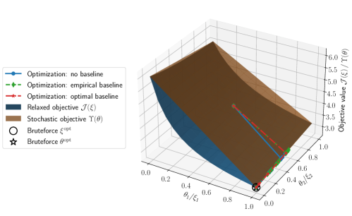
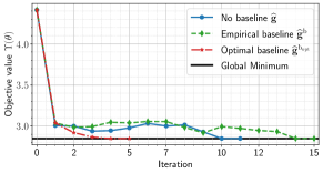
Figure 2: Left: surface plot of the objective function $\mathcal{J}$ of the relaxed OED problem and the objective function $\Upsilon$ of the corresponding stochastic OED problem. In each direction $15$ equally spaced points are taken to create the surface plots. Iterations of the optimization algorithm are shown on the surface plot for various choices of the baseline $b$. Right: value of the objective function $\Upsilon$ evaluated at each iteration of the algorithm until convergence. Brute-force results are obtained by searching over all $4$ possible values of the binary design $\mathbf{{\zeta}}\in\Omega_{\mathbf{{\zeta}}}$. The initial parameter $\mathbf{{\theta}}^{(0)}$ of the optimizer is set to $(0.5,0.5)^{\mkern-1.5mu\mathsf{T}}$, and the algorithm terminates when the magnitude of the projected gradient (pgtol) is lower than $10^{-8}$.

We note that, as explained in Section 3.2, the values of $\mathcal{J}(\mathbf{{\zeta}})$ and $\mathbf{{\theta}}$ coincide at the extremal points of the domain $[0,1]^{n_{\rm s}}$. Moreover, unlike the surface of the stochastic objective $\Upsilon$, the surface of the original objective function $\mathcal{J}$, evaluated at the relaxed design, flattens out for values of $\mathbf{{\theta}}_{1}$ greater than $0.5$. This behavior makes applying a sparsification procedure challenging when associated with traditional OED approaches.

While the performance varies slightly based on the choice of the baseline $b$, we note that, in general, the optimizer initially moves quickly toward a lower-dimensional space corresponding to lower values of the objective function $\Upsilon$ and then moves slowly toward a local optimum. We also note that since both candidate parameter values $(0,1)^{\mkern-1.5mu\mathsf{T}}$ and $(1,1)^{\mkern-1.5mu\mathsf{T}}$ have similar objective values, the optimizer moves slowly between them, since the value of the gradient in this direction is close to zero. If the optimizer is terminated before convergence (say after the first iteration where $\mathbf{{\theta}}_{1}$ is set to $1$ here), the returned value of $\mathbf{{\theta}}_{2}$ is in the interval $(0,1)$, which allows sampling estimates of $\mathbf{{\zeta}}_{1}^{\mkern-1.5mu\mathrm{opt}}$ from $\{0,1\}$, and the decision can be made based on the value of $\mathcal{J}$ or other decisions, such as budget constraints. Alternatively, one could modify (51) by adding a regularization term to enforce desired constraints. This will be explained further in Section 4.2.

Figure 3 shows the gradient of the stochastic objective function $\Upsilon$ evaluated (or approximated) at various choices of $\mathbf{{\theta}}$. The top-left panel show results using the exact formulation of the gradient (12). The top-right panel shows the gradient evaluated using (15). The lower two panels show evaluations of the gradient using (38) with an empirical choice baseline (52) and the estimate of the optimal baseline (49), respectively. These results show that the stochastic approximations of the gradient utilized in Algorithm 1 and Algorithm 2, better approximate the true gradient, given any realization of the parameter $\mathbf{{\theta}}$. However, the estimates with the baseline (both empirical choice and optimal estimate) exhibit much lower variability than the gradient evaluated without the baseline. This is also reflected by the performance of the optimization results in Figure 2.

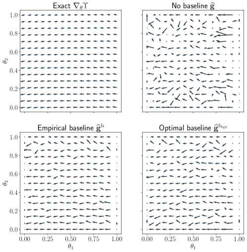
Figure 3: Evaluation of the gradient of the objective $\Upsilon(\mathbf{{\theta}}):=\mathbb{E}_{\xi\sim\mathbb{P}\left(\xi|\mathbf{{\theta}}\right)}{\Bigl{[}\mathcal{J(\xi)}\Bigr{]}}$, where $\mathcal{J}$ is defined by (50). Gradients are evaluated (or approximated) at $15$ equally spaced points in each direction. Top-left: gradient is evaluated exactly using (12). Top-right: gradient is approximated using (15). Bottom-left: gradient is approximated using (38), with $b$ set to (52). Bottom-right: gradient is approximated using (38), with $b$ evaluated using (49).

4.2 Experimental setup for an advection-diffusion problem

In this subsection we demonstrate the effectiveness of our proposed approach using an advection-diffusion model simulation that has been used extensively in the literature; see, for example, [39, 8, 9] and references therein.

The advection-diffusion model simulates the spatiotemporal evolution of a contaminant field $u=u(\mathbf{{x}},t)$ in a closed domain $\mathcal{D}$. Given a set of candidate locations to deploy sensors to measure the contaminant concentration, we seek the optimal subset of sensors that once deployed would enable inferring the initial distribution of the contaminant with minimum uncertainty. To this end, we seek the optimal subset of candidate sensors that minimized the A-optimality criterion, that is, the trace of the posterior covariance matrix.

We carry out numerical experiments in two settings with varying complexities. Specifically, we start with a setup where only $14$ candidate sensor locations are considered inside the domain $\mathcal{D}$. The number of possible combinations of active sensors in this case is $2^{14}=16,384$. Despite being large, this allows us to carry out a brute-force search. The purpose of the brute-force search here is to study the behavior of the proposed methodology and its capability in exploring the design space and utilizing any constraints properly, while seeking the optimal design. In particular, we can compare the quality of our solution with the global minimum in this case.

Model setup: advection-diffusion

In both sets of experiments, we use the same model setup. Specifically, the contaminant field $u=u(\mathbf{x},t)$ is governed by the advection-diffusion equation

(53) $$u_{t}-\kappa\Delta u+\mathbf{{v}}\cdot\nabla u =0\quad\text{in }\mathcal{D}\times[0,T],$$

$$u(x,\,0) =\theta\quad\text{in }\mathcal{D},$$

$$\kappa\nabla u\cdot\mathbf{{n}} =0\quad\text{on }\partial\mathcal{D}\times[0,T],$$

where $\kappa>0$ is the diffusivity, $T$ is the simulation final time, and $\mathbf{{v}}$ is the velocity field. The spatial domain here is $\mathcal{D}=[0,1]^{2}$, with two rectangular regions inside the domain simulating two buildings where the flow is not allowed to enter. Here, $\partial\mathcal{D}$ refers to the boundary of the domain, which includes both the external boundary and the walls of the two buildings. The velocity field $\mathbf{{v}}$ is assumed to be known and is obtained by solving a steady Navier–Stokes equation, with the side walls driving the flow; see [39] for further details.

To create a synthetic simulation, we use the initial distribution of contaminant shown in Figure 4 (left) as the ground truth.

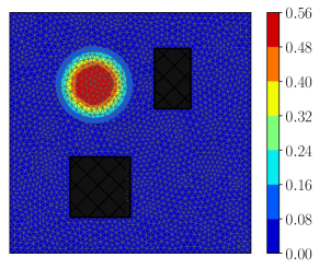
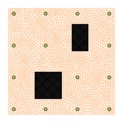
Figure 4: Advection-diffusion model domain, discretization, candidate sensor locations, and the true model parameter, in other words, the true initial condition. Left: The physical domain $\mathcal{D}$ including outer boundary and the two buildings, the model grid discretization, and the true model parameter. Right: Candidate observational sensor locations.

Observational setup

We consider a set of uniformly distributed candidate sensor locations (spatial observational gridpoints). Specifically, we consider $n_{\rm s}=14$ candidate sensor locations as described by Figure 4 (right), and we assume that the sensor locations do not change over time. An observation vector $\mathbf{y}$ represents the concentration of the contaminant at the sensor locations, at a set of predefined time instances $\{t_{1},\,t_{2},\,\ldots,\,t_{n_{t}}\}\subset[0,T]$. The observation times are set to $t_{1}\!+\!s\Delta t$, with initial observation time $t_{1}\!=\!1$; $\Delta t\!=\!0.2$ is the model simulation timestep; and $s=0,1,\ldots,20$. The result is $n_{t}=16$ observation time instances, over the simulation window $[0,\,T\!=\!4]$. The dimension of the observation space is thus $\textsc{N}_{\rm obs}=n_{\rm s}\times n_{t}$.

The observation error distribution is $\mathcal{N}\!\left({\mathbf{{0}}},{\mathbf{{\Gamma}}_{{\rm noise}}}\right)$, with $\mathbf{{\Gamma}}_{{\rm noise}}\in\mathbb{R}^{\textsc{N}_{\rm obs}\times\textsc{N}_{\rm obs}}$ describing spatiotemporal correlations of observational errors. We assume that observation errors are time-invariant and are calculated as follows. For simplicity, we assume that observation errors are uncorrelated, with fixed standard deviation; that is, the observation error covariance matrix takes the form $\mathbf{{\Gamma}}_{{\rm noise}}=\sigma_{\rm obs}^{2}\mathbf{{I}}$, where $\mathbf{{I}}\in\mathbb{R}^{\textsc{N}_{\rm obs}\times\textsc{N}_{\rm obs}}$ is the identity matrix. Here, we set the observation error variances to $\sigma_{\rm obs}\!=\!2.482\!\times\!10^{-2}$. This specific value is obtained by considering a noise level of $5\%$ of the maximum value of the contaminant concentration captured at all observation points, by running a simulation over $[0,T]$, using the ground truth of the model parameter; see Figure 4 (left).

Forward operator, adjoint operator, and the prior

The forward operator $\mathbf{F}$ maps the model parameter $\mathbf{{\theta}}$, here the model initial condition, to the observation space. Specifically, $\mathbf{F}$ represents a forward simulation over the interval $[0,T]$ followed by applying an observation operator (here, a restriction operator), to extract concentrations at sensor locations at observation time instances. The forward operator here is linear, and the adjoint is defined by using the Euclidean inner product weighted by the finite-element mass matrix $\mathbf{{M}}$ as $\mathbf{F}^{\mkern-1.5mu\mathsf{*}}:=\mathbf{{M}}^{\mkern-1.5mu\mathsf{-1}}\mathbf{{F}}^{\mkern-1.5mu\mathsf{T}}$; see [17] for further details.

The prior distribution of the parameter $\mathbf{{\theta}}$ is modeled by a Gaussian distribution $\mathcal{N}\!\left({\mathbf{{\theta}}_{\rm pr}},{\mathbf{{\Gamma}}_{{\rm pr}}}\right)$, where $\mathbf{{\Gamma}}_{{\rm pr}}$ is a discretization of $\mathcal{A}^{-2}$, with $\mathcal{A}$ being a Laplacian (following [17]).

4.3 The OED optimization problem

Now we define the design space and formulate the OED optimization problem. To find the best subset of candidate sensor locations, we assign a binary design variable $\mathbf{{\zeta}}_{i}$ to each candidate sensor location $x_{i}$, where $i=1,2,\ldots,n_{\rm s}$, and hence $\mathbf{{\zeta}}\in\{0,1\}^{n_{\rm s}}$. We aim to find a binary A-optimal design, that is, the minimizer of the trace of the posterior covariance matrix. Moreover, to promote sparsity of the design, we employ an $\ell_{0}$ penalty term $\Phi$. We thus define the objective function $\mathcal{J}$ for this problem as

(54) $$\mathcal{J}(\mathbf{{\zeta}})=\mathrm{Tr}\left(\left(\mathbf{{M}}^{\mkern-1.5mu\mathsf{-1}}\mathbf{{F}}^{\mkern-1.5mu\mathsf{T}}\mathbf{{\Gamma}}_{{\rm noise}}^{-1/2}\mathsf{diag}\left(\mathbf{{\zeta}}\right)\mathbf{{\Gamma}}_{{\rm noise}}^{-1/2}\mathbf{F}+\mathbf{{\Gamma}}_{{\rm pr}}^{-1}\right)^{\mkern-1.5mu\mathsf{-1}}\right)+\alpha\Phi(\mathbf{{\zeta}})\,,$$

where $\alpha$ is the user-defined penalty parameter. This parameter controls the level of sparsity that we desire to impose on the design. Specifically, we set $\Phi(\mathbf{{\zeta}}):=\left\|{\mathbf{{\zeta}}}\right\|_{0}$ to impose sparsity. On the other hand, if we have a specific budget $\lambda$, it would be more reasonable to define the penalty function as $\Phi(\mathbf{{\zeta}}):=\alpha\left|{\left\|{\mathbf{{\zeta}}}\right\|_{0}-\lambda}\right|=\alpha\left|{\sum_{i=1}^{n_{\rm s}}{\mathbf{{\zeta}}_{i}}-\lambda}\right|$. We will discuss these two cases in the following and in the numerical experiments. The stochastic optimization problem (9) is formulated given the definition of $\mathcal{J}$ in  (54) as

(55) $$\mathbf{{\theta}}^{\mkern-1.5mu\mathrm{opt}}=\operatorname*{arg\,min}_{\mathbf{{\theta}}\in[0,1]^{n_{\rm s}}}\mathbb{E}_{\mathbf{{\zeta}}\sim\mathbb{P}\left(\mathbf{{\zeta}}|\mathbf{{\theta}}\right)}{\Bigl{[}\mathrm{Tr}\left(\left(\mathbf{{M}}^{\mkern-1.5mu\mathsf{-1}}\mathbf{{F}}^{\mkern-1.5mu\mathsf{T}}\mathbf{{\Gamma}}_{{\rm noise}}^{-1/2}\mathsf{diag}\left(\mathbf{{\zeta}}\right)\mathbf{{\Gamma}}_{{\rm noise}}^{-1/2}\mathbf{F}+\mathbf{{\Gamma}}_{{\rm pr}}^{-1}\right)^{\mkern-1.5mu\mathsf{-1}}\right)+\alpha\Phi(\mathbf{{\zeta}})\Bigr{]}}\,,$$

where $\mathbb{P}\left(\mathbf{{\zeta}}|\mathbf{{\theta}}\right)$ is the multivariate Bernoulli distribution with PMF given by (8).

4.4 Numerical results with advection-diffusion model

The main goal of this set of experiments is to study the behavior of the proposed Algorithm 2 compared with the global solution of (55).

Solution by enumeration (brute-force) is carried out for all $2^{14}=16,384$ possible designs, and the corresponding value of $\mathcal{J}$ is recorded to identify the global solution of (55). In addition, we run Algorithm 2 with the maximum number of iterations set to $20$. We choose this tight number to test the performance of the stochastic optimization algorithm upon early termination. We choose the learning rate $\eta=0.25$ and set the gradient tolerance pgtol to $10^{-8}$. Each sensor is equipped with an initial probability $0.5$. This is employed by choosing the initial parameter $\mathbf{{\theta}}^{(0)}$ of the stochastic optimization algorithm to $\mathbf{{\theta}}^{(0)}=(0.5,0.5,\ldots,0.5)^{\mkern-1.5mu\mathsf{T}}$. In all experiments, we set the batch size for estimating the stochastic gradient to $32$ and the number of epochs for the optimal baseline to $10$.

The optimization algorithm returns samples from the multivariate Bernoulli distribution associated with the parameter $\mathbf{{\theta}}$ at the final step. Then, it picks $\mathbf{{\zeta}}^{\mkern-1.5mu\mathrm{opt}}$ as the sampled design associated with the smallest value of $\mathcal{J}$. We assume that the optimization procedure samples $10$ designs upon termination, from the final distribution. Note that all samples will be identical if the probability distribution is degenerate. In the numerical results discussed next, we show not only the final optimal design returned by the optimization procedure but also the sampled designs.

4.4.1 Results without penalty term

We start with numerical results obtained by setting the penalty parameter $\alpha=0$. Figure 5 shows the results of the brute-force search, along with results returned by Algorithm 1. Specifically, in Figure 5 (left), the value of $\mathcal{J}:=\mathrm{Tr}\left(\mathbf{{\Gamma}}_{{\rm post}}(\mathbf{{\zeta}})\right)$ is evaluated at each possible binary design $\mathbf{{\zeta}}$ and is shown on the y-axis. Candidate binary designs are grouped on the x-axis by the number of entries set to $1$, that is, the number of active sensors. In this setup, we have access to the value of $\mathcal{J}$ corresponding to all possible designs, and thus we can in fact evaluate $\Upsilon(\mathbf{{\theta}})\equiv\mathbb{E}_{\mathbf{{\zeta}}\sim\mathbb{P}\left(\mathbf{{\zeta}}|\mathbf{{\theta}}\right)}{\Bigl{[}\mathcal{J}(\mathbf{{\zeta}})\Bigr{]}}$ exactly, for any choice of the parameter $\mathbf{{\theta}}$. Of course, such an action is impossible in practice; however, we are interested in understanding the behavior of the optimization algorithm. Figure 5 (right) shows the value of $\Upsilon$ evaluated at the $k$th step of Algorithm 1.

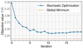
Figure 5: Results of the policy gradient Algorithm 1 compared with brute-force search of all candidate binary designs. No penalty is used here; that is, we set the penalty parameters $\alpha=0$. Left: candidate designs are grouped by the number of active sensors, on the x-axis, with the corresponding value of $\mathcal{J}$ displayed on the y-axis. Brute-force results are shown as blue dots. The results of Step 11 of Algorithm 1 with $m=10$ are shown as red stars, and the optimal solution returned from the algorithm is shown as a green circle. Right: The value of the stochastic objective $\Upsilon(\mathbf{{\theta}})$ evaluated at the $\mathbf{{\theta}}^{(k)}$ at each iteration $k$ of Algorithm 1.

In this setup, without any constraints on the number of sensors, the global optimal minimum is attained by $\mathbf{{\zeta}}^{\mkern-1.5mu\mathrm{opt}}=\mathbf{{1}}\in\mathbb{R}^{n_{\rm s}}$, that is, by activating all sensors. However, we note that increasing the number of sensors, say more than $8$, would add little to information gain from data. The reason is the similarity of the values of $\mathcal{J}$ for all designs with more than $8$ active sensors. The designs sampled from the final distribution obtained by Algorithm 1 are marked as red stars, which in this case are identical, showing that the final probability distribution is degenerate. The algorithm moves quickly toward a local minimum, but it fails to explore the space near the global optimum. This action is expected because of sampling error and the high variability of the estimator. As discussed in 3.5, improvements could be achieved by incorporating baseline in the objective function.

In Figure 6, we show results obtained by introducing baseline $b$ to the stochastic gradient estimator, as described by Algorithm 2. We show results with both the heuristic baseline estimate (52)  (Figure 6 (top)) and the optimal baseline estimate (47)  (Figure 6 (bottom)). Both Algorithm 1 and Algorithm 2 result in probability distributions (defined by $\mathbf{{\theta}}$) associated with small values. However, Algorithm 2 with the optimal baseline (47) outperforms both Algorithm 1, and Algorithm 2 with the heuristic baseline (52) and generates designs with significantly smaller objective values. Specifically, as shown in Figure 6 (bottom), the objective value $\mathcal{J}$ evaluated at the designs generated by Algorithm 2 are all similar and fall within $1\%$ of the global optimum.

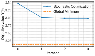
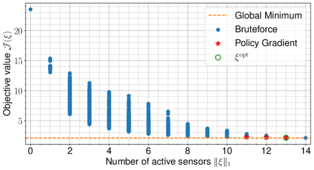
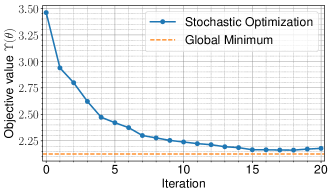
Figure 6: Same as Figure 5. Here, we show results of Algorithm 2, that is, stochastic optimization with the baseline. The top panels show results with the heuristic baseline estimate (52). The bottom panels show results with the optimal baseline estimate (47).

Evaluating the optimal baseline estimate, however, requires additional evaluations of $\mathcal{J}$. We monitor the number of additional evaluations of $\mathcal{J}$ carried out at each iteration of the optimizer. Note that we keep track of the values of $\mathcal{J}$ for each sampled design $\mathbf{{\zeta}}$ during the course of the algorithm. By doing so, we avoid any computational redundancy due to recalculating the objective function multiple times for the same design. Figure 7 shows the number of new function evaluations carried out at each step of the optimization algorithm.

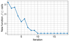
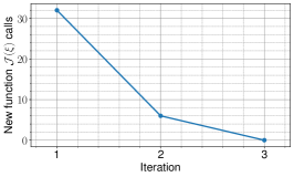
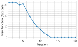
Figure 7: Number of new function evaluations carried out by the stochastic optimization algorithm. Left: results of Algorithm 1. Middle: results of Algorithm 2 with the heuristic baseline estimate (52). Right: results of Algorithm 2 with the optimal baseline estimate (47).

Figure 7 (left) suggests that, by using the heuristic baseline (52), the optimization algorithm converges quickly to a suboptimal probability space and does not require many additional function evaluations. A smaller step size $\eta$, in this case, might result in better performance. Conversely, comparing results in both Figure 7 (left) and Figure 7 (right), we notice that the computational cost, explained by the number of function evaluations, is not significantly different, especially after the first few iterations.

4.4.2 Results with sparsity constraint

To study the behavior of the optimization procedures in the presence $\ell_{0}$ sparsity constraints, we set the penalty function to $\Phi(\mathbf{{\zeta}}):=\left\|{\mathbf{{\zeta}}}\right\|_{0}$ and the regularization penalty parameter to $\alpha=1.0$. Here we do not concern ourselves with the choice of $\alpha$, and we leave it for the user to tune based on the application at hand and the required level of sparsity. Results are shown in Figure 8 and  Figure 9, respectively. For clarity we omit results obtained by the heuristic baseline.

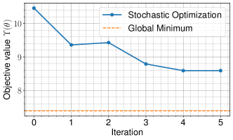
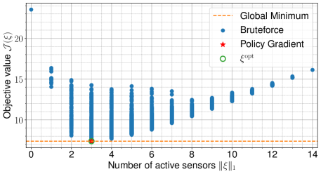
Figure 8: Results of the policy gradient procedures ( Algorithm 1, Algorithm 2), compared with the brute-force search of all candidate binary designs. Here, we set the sparsity penalty parameter to $\alpha=1.0$ and use a sparsity constraint, defined by $\Phi(\mathbf{{\zeta}}):=\left\|{\mathbf{{\zeta}}}\right\|_{0}$. Top: results of  Algorithm 1. Bottom:  Algorithm 2) with the optimal baseline estimate (47).

As suggested by Figure 8 (left), there is a unique global optimum design with only $3$ active sensors. Both Algorithm 1, and Algorithm 2 result in degenerate probability distributions. The global optimal design, however, is attained by utilizing the optimal baseline estimate as shown in Figure 8 (bottom). The computational cost of both algorithms, explained by the number of objective function evaluations, is shown in Figure 9.

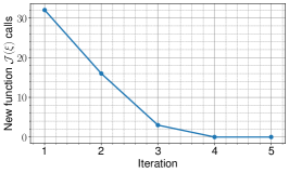
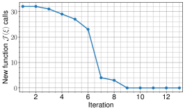
Figure 9: Similar to Figure 7. Here, we set the sparsity penalty parameter to $\alpha=1.0$ and use sparsity constraint, defined by $\Phi(\mathbf{{\zeta}}):=\left\|{\mathbf{{\zeta}}}\right\|_{0}$.

4.4.3 Results with fixed-budget constraint

To study the behavior of the optimization algorithms in the presence of an exact budget constraint $\left\|{\mathbf{{\zeta}}}\right\|_{0}=\lambda$, we carry out the same procedure, with the penalty function set to $\Phi(\mathbf{{\zeta}}):=\left|{\left\|{\mathbf{{\zeta}}}\right\|_{0}-\lambda}\right|$ and the regularization penalty parameter set to $\alpha=1.0$, and we set the budget to $\lambda=8$ sensors. Results are shown in Figure 10 and Figure 11, respectively. For clarity we omit results obtained by the heuristic baseline.

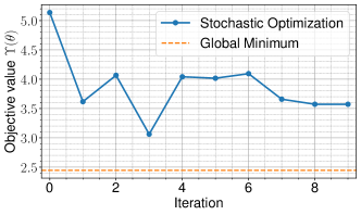
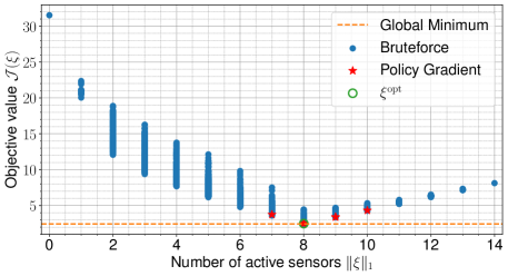
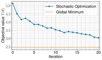
Figure 10: Results of the policy gradient procedures ( Algorithm 1 and Algorithm 2), compared with the brute-force search of all candidate binary designs. Here, we set the sparsity penalty parameter to $\alpha=1.0$ and use budget constraint, defined by $\Phi(\mathbf{{\zeta}}):=\left\|{\mathbf{{\zeta}}-\lambda}\right\|_{0}$, where $\lambda=8$. Top: results of  Algorithm 1. Bottom:  Algorithm 2) with the optimal baseline estimate (47).

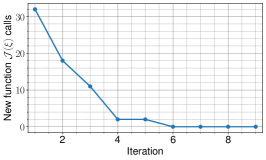
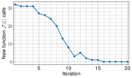
Figure 11: Similar to Figure 7. Here we set the sparsity penalty parameter to $\alpha=1.0$ and use the penalty constraint defined by $\Phi(\mathbf{{\zeta}}):=\left|{\left\|{\mathbf{{\zeta}}}\right\|_{0}-\lambda}\right|$, where $\lambda=8$.

We note that the performance of both Algorithm 1, and Algorithm 2 is consistent with and without sparsity constraints. Moreover, by incorporating the optimal baseline estimate (47) in Algorithm 2, at slight additional computational cost, the global optimum design is more likely to be discovered by the optimization algorithm.

4.4.4 Results with various learning rates

We conclude this section of experiments with results obtained by different learning rates. We use the setup in Section 4.4.3; that is, we assume an exact budget of $\lambda=8$ sensors and enforce it by setting the penalty function $\Phi(\mathbf{{\zeta}}):=\left\|{\mathbf{{\zeta}}}\right\|_{0}$ and the penalty parameter $\alpha=1$. Figure 12 shows results obtained by varying the learning rate $\eta$ in the optimization algorithm. Specifically, we show results obtained from Algorithm 2, with the optimal baseline estimate (47) and note that similar behavior was observed for the other settings used earlier in the paper.

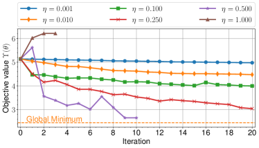
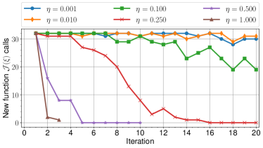
Figure 12: Similar to Figure 7. Here, we set the sparsity penalty parameter to $\alpha=1.0$ and use the budget constraint defined by $\Phi(\mathbf{{\zeta}}):=\left|{\left\|{\mathbf{{\zeta}}}\right\|_{0}-\lambda}\right|$, where $\lambda=8$.

Figure 12 (left) shows the value of the stochastic objective function corresponding to the parameter $\mathbf{{\theta}}^{(k)}$ at the $k$th iteration of the optimization algorithm for various choices of the learning rate. Figure 12 (right) shows the number of new calls to the function $\mathcal{J}$ made at each iteration of the algorithm. We note that by increasing the learning rate $\eta$, the algorithm tends to converge quickly and explore the space of probability distributions near the global optimal policy very quickly. However, this action is also associated with the risk of divergence. We note that $\eta=0.5$ is the best learning rate among the tested values.

In general, one can choose a small learning rate or even a decreasing sequence and run the optimization algorithm long enough to guarantee convergence to an optimal policy. Doing so, however, will likely increase the computational cost manifested in the number of evaluations of $\mathcal{J}$. This problem is widely known as the exploration-exploitation trade-off in the reinforcement learning literature. Finding an analytically optimal learning rate is beyond the scope of this paper and will be explored in separate work.

5 Discussion and Concluding Remarks

In this work, we presented a new approach for the optimal design of experiments for Bayesian inverse problems constrained by expensive mathematical models, such as partial differential equations. The regularized utility function is cast into a stochastic objective defined over the parameters of multivariate Bernoulli distribution. A policy gradient algorithm is used to optimize the new objective function and thus yields an approximately optimal probability distribution, that is, policy from which an approximately optimal design is sampled. The proposed approach does not require differentiability of the design utility function nor the penalty function generally employed to enforce sparsity or regularity conditions on the design. Hence, the computational cost of the proposed methods, in terms of the number of forward model solves, is much less than the cost required by traditional gradient-based approach for optimal experimental design. The decrease in computational cost is due mostly to the fact that the proposed method does not require evaluation of the simulation model for each entry of the gradient. Sparsity-enforcing penalty functions such as $\ell_{0}$ can be used directly, without the need to utilize a continuation procedure or apply a rounding technique.

The main open issue pertains to the optimal selection of the learning rate parameter. While using a decreasing sequence satisfying the Robbins–Monro conditions guarantees convergence of the proposed algorithm almost surely, such a choice may require many iterations before convergence to a degenerate optimal policy. This issue will be addressed in detail in separate work.

Note that the proposed stochastic formulation can be solved by other sample-based optimization algorithms, including sample average approximation [42, 47, 36]. The performance of these algorithms compared with that of the proposed algorithms will be also considered in separate works.

We note that utilizing traditional cost-reduction methods, including randomized matrix methods [12, 43, 44], and other reduced-order modeling approaches (see, e.g., [48, 23, 18, 11]), to reduce the cost of the OED criterion $\mathcal{J}$ apply to both the relaxed approach and our proposed approach equally. This shows that the proposed algorithms introduce massive computational savings to the OED solution process, compared with the traditional relaxation approach.

Appendix A Multivariate Bernoulli Distribution

The probabilities of a Bernoulli random variable $\mathbf{{\zeta}}\in\{0,1\}$ are described by

(56) $$\mathbb{P}\left(\mathbf{{\zeta}}=v|\mathbf{{\theta}}\right):=\begin{cases}\mathbf{{\theta}}&;\quad v=1\,,\\ 1-\mathbf{{\theta}}&;\quad v=0\,,\end{cases}$$

where $\mathbf{{\theta}}_{i}\in[0,1]$ can be thought of as the probability of success in a one-trial experiment. The probability mass function (PMF) of this variable takes the compact form $\mathbb{P}\left(\mathbf{{\zeta}}|\mathbf{{\theta}}\right)=\mathbf{{\theta}}^{\mathbf{{\zeta}}}\,(1-\mathbf{{\theta}})^{(1-\mathbf{{\zeta}})}$. Moreover, the following identity holds:

(57) $$\frac{\partial{\mathbb{P}\left(\mathbf{{\zeta}}|\mathbf{{\theta}}\right)}}{\partial{\mathbf{{\theta}}}}=(-1)^{1-\mathbf{{\zeta}})}\,.$$

Assuming $\mathbf{{\zeta}}_{i},\,i=1,2,\ldots,n_{\rm s}$ are mutually independent Bernoulli random variables with respective success probabilities $\mathbf{{\theta}}_{i},\,i=1,2,\ldots,n_{\rm s}$, then the joint probability mass function of the random variable $\mathbf{{\zeta}}=(\mathbf{{\zeta}}_{1},\mathbf{{\zeta}}_{2},\ldots,\mathbf{{\zeta}}_{n_{\rm s}})^{\mkern-1.5mu\mathsf{T}}$, parameterized by $\mathbf{{\theta}}=(\mathbf{{\theta}}_{1},\mathbf{{\theta}}_{2},\ldots,\mathbf{{\theta}}_{n_{\rm s}})^{\mkern-1.5mu\mathsf{T}}$, takes the form

(58) $$\mathbb{P}\left(\mathbf{{\zeta}}|\mathbf{{\theta}}\right)=\prod_{i=1}^{n_{\rm s}}{\mathbf{{\theta}}_{i}^{\mathbf{{\zeta}}_{i}}\,\left(1-\mathbf{{\theta}}_{i}\right)^{1-\mathbf{{\zeta}}_{i}}}\equiv\prod_{i=1}^{n_{\rm s}}\Bigl{(}{\mathbf{{\theta}}_{i}{\mathbf{{\zeta}}_{i}}\,+\left(1-\mathbf{{\theta}}_{i}\right)\left(1-\mathbf{{\zeta}}_{i}\right)}\Bigr{)}\,,\quad\mathbf{{\zeta}}_{i}\in\{0,1\}\,.$$

By using (57), the first-order derivative of (58) w.r.t the parameters $\mathbf{{\theta}}_{i}$ is described by

(59) $$\frac{\partial{\mathbb{P}\left(\mathbf{{\zeta}}|\mathbf{{\theta}}\right)}}{\partial{\mathbf{{\theta}}_{j}}} =\frac{\partial{}}{\partial{\mathbf{{\theta}}_{j}}}\left(\mathbf{{\theta}}_{j}^{\mathbf{{\zeta}}_{j}}\,\left(1-\mathbf{{\theta}}_{j}\right)^{1-\mathbf{{\zeta}}_{j}}\prod_{\begin{subarray}{c}i=1\\ i\neq j\end{subarray}}^{n_{\rm s}}{\mathbf{{\theta}}_{i}^{\mathbf{{\zeta}}_{i}}\left(1-\mathbf{{\theta}}_{i}\right)^{1-\mathbf{{\zeta}}_{i}}}\right)=(-1)^{1-\mathbf{{\zeta}}_{j}}\prod_{\begin{subarray}{c}i=1\\ i\neq j\end{subarray}}^{n_{\rm s}}{\mathbf{{\theta}}_{i}^{\mathbf{{\zeta}}_{i}}\left(1-\mathbf{{\theta}}_{i}\right)^{1-\mathbf{{\zeta}}_{i}}}\,.$$

Thus, the gradient can be written as

(60) $$\nabla_{\mathbf{{\theta}}}\,\mathbb{P}\left(\mathbf{{\zeta}}|\mathbf{{\theta}}\right)=\sum_{j=1}^{n_{\rm s}}\frac{\partial{\mathbb{P}\left(\mathbf{{\zeta}}|\mathbf{{\theta}}\right)}}{\partial{\mathbf{{\theta}}_{j}}}=\sum_{j=1}^{n_{\rm s}}(-1)^{1-\mathbf{{\zeta}}_{j}}\prod_{\begin{subarray}{c}i=1\\ i\neq j\end{subarray}}^{n_{\rm s}}{\mathbf{{\theta}}_{i}^{\mathbf{{\zeta}}_{i}}\left(1-\mathbf{{\theta}}_{i}\right)^{1-\mathbf{{\zeta}}_{i}}}\mathbf{{e}}_{j}\,.$$

Note that the derivative given by (59) is the (signed) conditional probability of $\mathbf{{\zeta}}$ conditioned by $\mathbf{{\zeta}}_{j}$ and $\mathbf{{\theta}}_{j}$, respectively. The second-order derivatives follow as

(61) $$\frac{\partial^{2}{\mathbb{P}\left(\mathbf{{\zeta}}|\mathbf{{\theta}}\right)}}{\partial{\mathbf{{\theta}}_{k}}\,\partial{\mathbf{{\theta}}_{j}}} =(1-\delta_{kj})(-1)^{2-\mathbf{{\zeta}}_{j}-\mathbf{{\zeta}}_{k}}\prod_{\begin{subarray}{c}i=1\\ i\notin\{j,k\}\end{subarray}}^{n_{\rm s}}{\mathbf{{\theta}}_{i}^{\mathbf{{\zeta}}_{i}}\,\left(1-\mathbf{{\theta}}_{i}\right)^{1-\mathbf{{\zeta}}_{i}}}\,,$$

where $\delta_{kj}$ is the standard Kronecker delta function. The gradient of the log-probabilities, that is, the score function, of the multivariate Bernoulli PMF (58), is given by

(62) $$\nabla_{\mathbf{{\theta}}}\log{\mathbb{P}\left(\mathbf{{\zeta}}|\mathbf{{\theta}}\right)} =\nabla_{\mathbf{{\theta}}}\log{\prod_{i=1}^{n_{\rm s}}{\mathbf{{\theta}}_{i}^{\mathbf{{\zeta}}_{i}}\,\left(1-\mathbf{{\theta}}_{i}\right)^{1-\mathbf{{\zeta}}_{i}}}}=\sum_{i=1}^{n_{\rm s}}\nabla_{\mathbf{{\theta}}}\log{\mathbf{{\theta}}_{i}^{\mathbf{{\zeta}}_{i}}}+\sum_{i=1}^{n_{\rm s}}\nabla_{\mathbf{{\theta}}}\log{\left(1-\mathbf{{\theta}}_{i}\right)^{1-\mathbf{{\zeta}}_{i}}}$$

$$=\sum_{i=1}^{n_{\rm s}}{\mathbf{{\zeta}}_{i}}\nabla_{\mathbf{{\theta}}}\log{\mathbf{{\theta}}_{i}}+\sum_{i=1}^{n_{\rm s}}(1-\mathbf{{\zeta}}_{i})\nabla_{\mathbf{{\theta}}}\log{\left(1-\mathbf{{\theta}}_{i}\right)}=\sum_{i=1}^{n_{\rm s}}\left(\frac{\mathbf{{\zeta}}_{i}}{\mathbf{{\theta}}_{i}}+\frac{\mathbf{{\zeta}}_{i}-1}{1-\mathbf{{\theta}}_{i}}\right)\,\mathbf{{e}}_{i}\,.$$

It follows immediately from (62) that

(63) $$\nabla_{\mathbf{{\theta}}}\nabla_{\mathbf{{\theta}}}\log{\mathbb{P}\left(\mathbf{{\zeta}}|\mathbf{{\theta}}\right)} =\sum_{i=1}^{n_{\rm s}}\left(\frac{-\mathbf{{\zeta}}_{i}}{\mathbf{{\theta}}_{i}^{2}}-\frac{1-\mathbf{{\zeta}}_{i}}{(1-\mathbf{{\theta}}_{i})^{2}}\right)\,\mathbf{{e}}_{i}\mathbf{{e}}_{i}^{\mkern-1.5mu\mathsf{T}}$$

$$\nabla_{\mathbf{{\theta}}}\log{\mathbb{P}\left(\mathbf{{\zeta}}|\mathbf{{\theta}}\right)}\left(\nabla_{\mathbf{{\theta}}}\log{\mathbb{P}\left(\mathbf{{\zeta}}|\mathbf{{\theta}}\right)}\right)^{\mkern-1.5mu\mathsf{T}} =\sum_{i=1}^{n_{\rm s}}\sum_{j=1}^{n_{\rm s}}\left(\frac{\mathbf{{\zeta}}_{i}}{\mathbf{{\theta}}_{i}}-\frac{1-\mathbf{{\zeta}}_{i}}{1-\mathbf{{\theta}}_{i}}\right)\left(\frac{\mathbf{{\zeta}}_{j}}{\mathbf{{\theta}}_{j}}-\frac{1-\mathbf{{\zeta}}_{j}}{1-\mathbf{{\theta}}_{j}}\right)\,\mathbf{{e}}_{i}\mathbf{{e}}_{j}^{\mkern-1.5mu\mathsf{T}}.$$

In the rest of this Appendix, we prove some identities essential for convergence analysis of the algorithms proposed in this work. We start with the following basic relations. First note that $\mathbb{E}{\Bigl{[}\mathbf{{\zeta}}_{i}\mathbf{{\zeta}}_{j}\Bigr{]}}=\mathsf{cov}{\Bigl{(}\mathbf{{\zeta}}_{i},\,\mathbf{{\zeta}}_{j}\Bigr{)}}+\mathbb{E}{\Bigl{[}\mathbf{{\zeta}}_{i}\Bigr{]}}\mathbb{E}{\Bigl{[}\mathbf{{\zeta}}_{j}\Bigr{]}}=\delta_{ij}\mathbf{{\theta}}_{i}(1-\mathbf{{\theta}}_{i})+\mathbf{{\theta}}_{i}\mathbf{{\theta}}_{j}$. This means that $\mathbb{E}{\Bigl{[}\mathbf{{\zeta}}_{i}^{2}\Bigr{]}}=\mathbb{E}{\Bigl{[}\mathbf{{\zeta}}_{i}\Bigr{]}}=\mathbf{{\theta}}_{i}$ and $\mathbb{E}{\Bigl{[}\mathbf{{\zeta}}_{i}\mathbf{{\zeta}}_{j}\Bigr{]}}=\mathbf{{\theta}}_{i}\mathbf{{\theta}}_{j}\,\forall i\neq j$. Similarly, $\mathbb{E}{\Bigl{[}\mathbf{{\zeta}}_{i}(\mathbf{{\zeta}}_{j}-1)\Bigr{]}}=\mathbb{E}{\Bigl{[}\mathbf{{\zeta}}_{i}\mathbf{{\zeta}}_{j}\Bigr{]}}-\mathbb{E}{\Bigl{[}\mathbf{{\zeta}}_{i}\Bigr{]}}=\delta_{ij}\mathbf{{\theta}}_{i}(1-\mathbf{{\theta}}_{i})+\mathbf{{\theta}}_{i}\mathbf{{\theta}}_{j}-\mathbf{{\theta}}_{i}\,,$ and $\mathbb{E}{\Bigl{[}(\mathbf{{\zeta}}_{i}-1)(\mathbf{{\zeta}}_{j}-1)\Bigr{]}}=\mathbb{E}{\Bigl{[}\mathbf{{\zeta}}_{i}\mathbf{{\zeta}}_{j}\Bigr{]}}-\mathbf{{\theta}}_{i}-\mathbf{{\theta}}_{j}+1=\delta_{ij}\mathbf{{\theta}}_{i}(1-\mathbf{{\theta}}_{i})+\mathbf{{\theta}}_{i}\mathbf{{\theta}}_{j}-\mathbf{{\theta}}_{i}-\mathbf{{\theta}}_{j}+1\,.$ We can summarize these identities as follows:

(64) $$\mathbb{E}{\Bigl{[}\mathbf{{\zeta}}_{i}\mathbf{{\zeta}}_{j}\Bigr{]}} =\begin{cases}\mathbf{{\theta}}_{i},\,&\,i=j\\ \mathbf{{\theta}}_{i}\mathbf{{\theta}}_{j},\,&\,i\neq j\end{cases}\,,$$

$$\mathbb{E}{\Bigl{[}\mathbf{{\zeta}}_{i}(\mathbf{{\zeta}}_{j}\!-\!1)\Bigr{]}} =\begin{cases}0,\,&\,i=j\\ \mathbf{{\theta}}_{i}(\mathbf{{\theta}}_{j}\!-\!1),\,&\,i\neq j\end{cases}\,,$$

$$\mathbb{E}{\Bigl{[}(\mathbf{{\zeta}}_{i}\!-\!1)(\mathbf{{\zeta}}_{j}\!-\!1)\Bigr{]}} =\begin{cases}1\!-\!\mathbf{{\theta}}_{i},\,&\,i=j\\ (1-\mathbf{{\theta}}_{i})(1-\mathbf{{\theta}}_{j}),\,&\,i\neq j\end{cases}\,.$$

Lemma A.1.

Let $\mathbf{{\zeta}}\in\Omega_{\mathbf{{\zeta}}}:=\{0,1\}^{n_{\rm s}}$ be a random variable following the joint Bernoulli distribution (58), and assume that $\mathsf{var}{(\mathbf{{\zeta}})}$ is the total variance operator that evaluates the trace of the variance-covariance matrix of the random variable $\mathbf{{\zeta}}$. Then the following identities hold:

(65) $$\mathbb{E}{\Bigl{[}\nabla_{\mathbf{{\theta}}}\log{\mathbb{P}\left(\mathbf{{\zeta}}|\mathbf{{\theta}}\right)}\Bigr{]}}=0\,;\qquad\mathsf{var}\Bigl{(}\nabla_{\mathbf{{\theta}}}\log{\mathbb{P}\left(\mathbf{{\zeta}}|\mathbf{{\theta}}\right)}\Bigr{)}=\sum_{i=1}^{n_{\rm s}}\frac{1}{\mathbf{{\theta}}_{i}-\mathbf{{\theta}}_{i}^{2}}\,.$$

Proof A.2.

The first identity follows as

(66) $$\mathbb{E}{\Bigl{[}\nabla_{\mathbf{{\theta}}}\log{\mathbb{P}\left(\mathbf{{\zeta}}|\mathbf{{\theta}}\right)}\Bigr{]}}=\sum_{\mathbf{{\zeta}}}\nabla_{\mathbf{{\theta}}}\log{\mathbb{P}\left(\mathbf{{\zeta}}|\mathbf{{\theta}}\right)}\mathbb{P}\left(\mathbf{{\zeta}}|\mathbf{{\theta}}\right)=\sum_{\mathbf{{\zeta}}}\nabla_{\mathbf{{\theta}}}\mathbb{P}\left(\mathbf{{\zeta}}|\mathbf{{\theta}}\right)=\nabla_{\mathbf{{\theta}}}\sum_{\mathbf{{\zeta}}}\mathbb{P}\left(\mathbf{{\zeta}}|\mathbf{{\theta}}\right)=0\,.$$

By definition of the covariance matrix, and since $\mathbb{E}{\Bigl{[}\nabla_{\mathbf{{\theta}}}\log{\mathbb{P}\left(\mathbf{{\zeta}}|\mathbf{{\theta}}\right)}\Bigr{]}}=0$, then

(67) $$\mathsf{var}\Bigl{(}\nabla_{\mathbf{{\theta}}}\log{\mathbb{P}\left(\mathbf{{\zeta}}|\mathbf{{\theta}}\right)}\Bigr{)} =\mathrm{Tr}\left(\mathsf{cov}{\Bigl{(}\nabla_{\mathbf{{\theta}}}\log{\mathbb{P}\left(\mathbf{{\zeta}}|\mathbf{{\theta}}\right)},\nabla_{\mathbf{{\theta}}}\log{\mathbb{P}\left(\mathbf{{\zeta}}|\mathbf{{\theta}}\right)}\Bigr{)}}\right)$$

$$=\mathrm{Tr}\left(\mathbb{E}{\Bigl{[}\left(\nabla_{\mathbf{{\theta}}}\log{\mathbb{P}\left(\mathbf{{\zeta}}|\mathbf{{\theta}}\right)}\right)\left(\nabla_{\mathbf{{\theta}}}\log{\mathbb{P}\left(\mathbf{{\zeta}}|\mathbf{{\theta}}\right)}\right)^{\mkern-1.5mu\mathsf{T}}\Bigr{]}}\right)$$

$$=\mathbb{E}{\Bigl{[}\mathrm{Tr}\left(\left(\nabla_{\mathbf{{\theta}}}\log{\mathbb{P}\left(\mathbf{{\zeta}}|\mathbf{{\theta}}\right)}\right)\left(\nabla_{\mathbf{{\theta}}}\log{\mathbb{P}\left(\mathbf{{\zeta}}|\mathbf{{\theta}}\right)}\right)^{\mkern-1.5mu\mathsf{T}}\right)\Bigr{]}}$$

$$=\mathbb{E}{\Bigl{[}\left(\nabla_{\mathbf{{\theta}}}\log{\mathbb{P}\left(\mathbf{{\zeta}}|\mathbf{{\theta}}\right)}\right)^{\mkern-1.5mu\mathsf{T}}\left(\nabla_{\mathbf{{\theta}}}\log{\mathbb{P}\left(\mathbf{{\zeta}}|\mathbf{{\theta}}\right)}\right)\Bigr{]}}\,,$$

where we utilized the circular property of the trace operator and the fact that the matrix trace is a linear operator. Thus,

(68) $$\mathsf{var}\Bigl{(}\nabla_{\mathbf{{\theta}}}\log{\mathbb{P}\left(\mathbf{{\zeta}}|\mathbf{{\theta}}\right)}\Bigr{)} =\mathbb{E}{\Bigl{[}\left(\nabla_{\mathbf{{\theta}}}\log{\mathbb{P}\left(\mathbf{{\zeta}}|\mathbf{{\theta}}\right)}\right)^{\mkern-1.5mu\mathsf{T}}\left(\nabla_{\mathbf{{\theta}}}\log{\mathbb{P}\left(\mathbf{{\zeta}}|\mathbf{{\theta}}\right)}\right)\Bigr{]}}$$

$$=\mathbb{E}{\Bigl{[}\sum_{i=1}^{n_{\rm s}}\left(\frac{\partial{\log{\mathbb{P}\left(\mathbf{{\zeta}}|\mathbf{{\theta}}_{i}\right)}}}{\partial{\mathbf{{\theta}}_{i}}}\right)^{2}\Bigr{]}}=\mathbb{E}{\Bigl{[}\sum_{i=1}^{n_{\rm s}}\left(\frac{\mathbf{{\zeta}}_{i}}{\mathbf{{\theta}}_{i}}+\frac{\mathbf{{\zeta}}_{i}-1}{1-\mathbf{{\theta}}_{i}}\right)^{2}\Bigr{]}}$$

$$=\mathbb{E}{\Bigl{[}\sum_{i=1}^{n_{\rm s}}\left(\frac{\mathbf{{\zeta}}_{i}^{2}}{\mathbf{{\theta}}_{i}^{2}}+2\frac{\mathbf{{\zeta}}_{i}^{2}-\mathbf{{\zeta}}_{i}}{\mathbf{{\theta}}_{i}-\mathbf{{\theta}}_{i}^{2}}+\frac{\mathbf{{\zeta}}_{i}^{2}-2\mathbf{{\zeta}}_{i}+1}{(1-\mathbf{{\theta}}_{i})^{2}}\right)\Bigr{]}}$$

$$=\sum_{i=1}^{n_{\rm s}}\left(\frac{\mathbb{E}{\Bigl{[}\mathbf{{\zeta}}_{i}^{2}\Bigr{]}}}{\mathbf{{\theta}}_{i}^{2}}+\frac{\mathbb{E}{\Bigl{[}\mathbf{{\zeta}}_{i}^{2}\Bigr{]}}-2\mathbb{E}{\Bigl{[}\mathbf{{\zeta}}_{i}\Bigr{]}}+1}{(1-\mathbf{{\theta}}_{i})^{2}}\right)=\sum_{i=1}^{n_{\rm s}}\left(\frac{\mathbf{{\theta}}_{i}}{\mathbf{{\theta}}_{i}^{2}}+\frac{\mathbf{{\theta}}_{i}-2\mathbf{{\theta}}_{i}+1}{(1-\mathbf{{\theta}}_{i})^{2}}\right)$$

$$=\sum_{i=1}^{n_{\rm s}}\left(\frac{1}{\mathbf{{\theta}}_{i}}+\frac{1-\mathbf{{\theta}}_{i}}{(1-\mathbf{{\theta}}_{i})^{2}}\right)=\sum_{i=1}^{n_{\rm s}}\left(\frac{1}{\mathbf{{\theta}}_{i}}+\frac{1}{1-\mathbf{{\theta}}_{i}}\right)=\sum_{i=1}^{n_{\rm s}}\frac{1}{\mathbf{{\theta}}_{i}-\mathbf{{\theta}}_{i}^{2}}\,,$$

where we used the fact that $\mathbb{E}{\Bigl{[}\mathbf{{\zeta}}_{i}^{2}\Bigr{]}}=\mathbf{{\theta}}_{i}$, as shown by (64). This is also obvious since $\mathbf{{\zeta}}^{2}=\mathbf{{\zeta}}$.

Lemma A.3.

Let $\mathbf{{\zeta}}\in\Omega_{\mathbf{{\zeta}}}:=\{0,1\}^{n_{\rm s}}$ be a random variable following the joint Bernoulli distribution (58). Then for any $\mathbf{{\zeta}}\in\Omega_{\mathbf{{\zeta}}}$, the following bounds hold:

(69) $$\left\|{\nabla_{\mathbf{{\theta}}}\,\mathbb{P}\left(\mathbf{{\zeta}}|\mathbf{{\theta}}\right)}\right\| \leq\sqrt{n_{\rm s}}\,\max\limits_{j=1,\ldots,n_{\rm s}}\,\min\limits_{\begin{subarray}{c}i=1,\ldots,n_{\rm s}\\ k\neq j\end{subarray}}\mathbb{P}\left(\mathbf{{\zeta}}_{i}|\mathbf{{\theta}}_{i}\right)$$

(70) $$\mathbb{E}_{\mathbf{{\zeta}}}{\Bigl{[}\left\|{\nabla_{\mathbf{{\theta}}}\log{\mathbb{P}\left(\mathbf{{\zeta}}|\mathbf{{\theta}}\right)}}\right\|^{2}\Bigr{]}}\equiv\mathsf{var}\Bigl{(}\nabla_{\mathbf{{\theta}}}{\log{\mathbb{P}\left(\mathbf{{\zeta}}|\mathbf{{\theta}}\right)}}\Bigr{)} \leq\frac{n_{\rm s}}{\min\limits_{i}\mathbf{{\theta}}}+\frac{n_{\rm s}}{1-\max\limits_{i}\mathbf{{\theta}}}\,.$$

Proof A.4.

(71) $$\left\|{\nabla_{\mathbf{{\theta}}}\,\mathbb{P}\left(\mathbf{{\zeta}}|\mathbf{{\theta}}\right)}\right\|^{2} =\left\|{\sum_{j=1}^{n_{\rm s}}(-1)^{1-\mathbf{{\zeta}}_{j}}\prod_{\begin{subarray}{c}i=1\\ k\neq j\end{subarray}}^{n_{\rm s}}{\mathbf{{\theta}}_{i}^{\mathbf{{\zeta}}_{i}}\left(1-\mathbf{{\theta}}_{i}\right)^{1-\mathbf{{\zeta}}_{i}}}\mathbf{{e}}_{j}}\right\|^{2}$$

$$\leq\sum_{j=1}^{n_{\rm s}}\left|(-1)^{1-\mathbf{{\zeta}}_{j}}\right|\left(\prod_{\begin{subarray}{c}i=1\\ k\neq j\end{subarray}}^{n_{\rm s}}{\mathbf{{\theta}}_{i}^{\mathbf{{\zeta}}_{i}}\left(1-\mathbf{{\theta}}_{i}\right)^{1-\mathbf{{\zeta}}_{i}}}\right)^{2}$$

$$\leq\sum_{j=1}^{n_{\rm s}}\,\min\limits_{\begin{subarray}{c}i=1,\ldots,n_{\rm s}\\ k\neq j\end{subarray}}\left(\mathbb{P}\left(\mathbf{{\zeta}}_{i}|\mathbf{{\theta}}_{i}\right)\right)^{2}\leq n_{\rm s}\,\max\limits_{j=1,\ldots,n_{\rm s}}\min\limits_{\begin{subarray}{c}i=1,\ldots,n_{\rm s}\\ k\neq j\end{subarray}}\left(\mathbb{P}\left(\mathbf{{\zeta}}_{i}|\mathbf{{\theta}}_{i}\right)\right)^{2}\,,$$

which prove the first inequality (69). By utilizing (62), we have

(72) $$\left\|{\nabla_{\mathbf{{\theta}}}\log{\mathbb{P}\left(\mathbf{{\zeta}}|\mathbf{{\theta}}\right)}}\right\|^{2} =\left\|{\sum_{i=1}^{n_{\rm s}}\left(\frac{\mathbf{{\zeta}}_{i}}{\mathbf{{\theta}}_{i}}+\frac{\mathbf{{\zeta}}_{i}-1}{1-\mathbf{{\theta}}_{i}}\right)\,\mathbf{{e}}_{i}}\right\|^{2}=\sum_{i=1}^{n_{\rm s}}\left(\frac{\mathbf{{\zeta}}_{i}}{\mathbf{{\theta}}_{i}}+\frac{\mathbf{{\zeta}}_{i}-1}{1-\mathbf{{\theta}}_{i}}\right)^{2}$$

$$=\sum_{i=1}^{n_{\rm s}}\left(\frac{\mathbf{{\zeta}}_{i}^{2}}{\mathbf{{\theta}}_{i}^{2}}+2\frac{\mathbf{{\zeta}}_{i}(\mathbf{{\zeta}}_{i}-1)}{\mathbf{{\theta}}_{i}(1-\mathbf{{\theta}}_{i})}+\frac{\left(\mathbf{{\zeta}}_{i}-1\right)^{2}}{\left(1-\mathbf{{\theta}}_{i}\right)^{2}}\right)=\sum_{i=1}^{n_{\rm s}}\left(\frac{\mathbf{{\zeta}}_{i}}{\mathbf{{\theta}}_{i}^{2}}+\frac{\mathbf{{\zeta}}_{i}-1}{\left(1-\mathbf{{\theta}}_{i}\right)^{2}}\right)\,.$$

where the last relation follows given the fact that $\mathbf{{\zeta}}_{i}\in\{0,1\}$, and hence $\mathbf{{\zeta}}_{i}^{2}=\mathbf{{\zeta}}_{i}\,,\forall\,i=1,2,\ldots,n_{\rm s}$. Taking the expectation of both sides, we get

(73) $$\mathbb{E}_{\mathbf{{\zeta}}}{\Bigl{[}\left\|{\nabla_{\mathbf{{\theta}}}\log{\mathbb{P}\left(\mathbf{{\zeta}}|\mathbf{{\theta}}\right)}}\right\|^{2}\Bigr{]}} =\mathbb{E}_{\mathbf{{\zeta}}}{\Bigl{[}\sum_{i=1}^{n_{\rm s}}\left(\frac{\mathbf{{\zeta}}_{i}}{\mathbf{{\theta}}_{i}^{2}}+\frac{\mathbf{{\zeta}}_{i}-1}{\left(1-\mathbf{{\theta}}_{i}\right)^{2}}\right)\Bigr{]}}=\sum_{i=1}^{n_{\rm s}}\left(\frac{\mathbb{E}{\Bigl{[}\mathbf{{\zeta}}_{i}\Bigr{]}}}{\mathbf{{\theta}}_{i}^{2}}+\frac{\mathbb{E}{\Bigl{[}\mathbf{{\zeta}}_{i}\Bigr{]}}-1}{\left(1-\mathbf{{\theta}}_{i}\right)^{2}}\right)$$

$$=\sum_{i=1}^{n_{\rm s}}\left(\frac{\mathbf{{\theta}}_{i}}{\mathbf{{\theta}}_{i}^{2}}+\frac{\mathbf{{\theta}}_{i}-1}{\left(1-\mathbf{{\theta}}_{i}\right)^{2}}\right)=\sum_{i=1}^{n_{\rm s}}\left(\frac{1}{\mathbf{{\theta}}_{i}}+\frac{1}{\left(1-\mathbf{{\theta}}_{i}\right)}\right)$$

$$=\sum_{i=1}^{n_{\rm s}}\frac{1}{\mathbf{{\theta}}_{i}}+\sum_{i=1}^{n_{\rm s}}\frac{1}{\left(1-\mathbf{{\theta}}_{i}\right)}\leq\frac{n_{\rm s}}{\min\limits_{i}\mathbf{{\theta}}}+\frac{n_{\rm s}}{1-\max\limits_{i}\mathbf{{\theta}}}\,,$$

which completes the proof of (70).    

The submitted manuscript has been created by UChicago Argonne, LLC, Operator of Argonne National Laboratory (“Argonne”). Argonne, a U.S. Department of Energy Office of Science laboratory, is operated under Contract No. DE-AC02-06CH11357. The U.S. Government retains for itself, and others acting on its behalf, a paid-up nonexclusive, irrevocable worldwide license in said article to reproduce, prepare derivative works, distribute copies to the public, and perform publicly and display publicly, by or on behalf of the Government. The Department of Energy will provide public access to these results of federally sponsored research in accordance with the DOE Public Access Plan. http://energy.gov/downloads/doe-public-access-plan.

References

- [1] A. Alexanderian, Optimal experimental design for bayesian inverse problems governed by pdes: A review, arXiv preprint arXiv:2005.12998, (2020).
- [2] A. Alexanderian, P. J. Gloor, O. Ghattas, et al., On Bayesian A-and D-optimal experimental designs in infinite dimensions, Bayesian Analysis, 11 (2016), pp. 671–695.
- [3] A. Alexanderian, N. Petra, G. Stadler, and O. Ghattas, A-optimal design of experiments for infinite-dimensional Bayesian linear inverse problems with regularized -sparsification, SIAM Journal on Scientific Computing, 36 (2014), pp. A2122–A2148, https://doi.org/10.1137/130933381.
- [4] A. Alexanderian, N. Petra, G. Stadler, and O. Ghattas, A fast and scalable method for A-optimal design of experiments for infinite-dimensional Bayesian nonlinear inverse problems, SIAM Journal on Scientific Computing, 38 (2016), pp. A243–A272, https://doi.org/10.1137/140992564, http://dx.doi.org/10.1137/140992564.
- [5] A. Alexanderian and A. K. Saibaba, Efficient D-optimal design of experiments for infinite-dimensional Bayesian linear inverse problems, Submitted, (2017), https://arxiv.org/abs/1711.05878.
- [6] B. Arouna, Adaptative monte carlo method, a variance reduction technique, Monte Carlo Methods and Applications, 10 (2004), pp. 1–24.
- [7] A. Attia, DOERL: design of experiments using reinforcement learning, 2020, https://gitlab.com/ahmedattia/doerl.
- [8] A. Attia, A. Alexanderian, and A. K. Saibaba, Goal-oriented optimal design of experiments for large-scale Bayesian linear inverse problems, Inverse Problems, 34 (2018), p. 095009, http://stacks.iop.org/0266-5611/34/i=9/a=095009.
- [9] A. Attia and E. Constantinescu, Optimal experimental design for inverse problems in the presence of observation correlations, arXiv preprint arXiv:2007.14476, (2020).
- [10] A. Attia and A. Sandu, A hybrid Monte Carlo sampling filter for non-Gaussian data assimilation, AIMS Geosciences, 1 (2015), pp. 4–1–78, https://doi.org/http://dx.doi.org/10.3934/geosci.2015.1.41, http://www.aimspress.com/geosciences/article/574.html.
- [11] A. Attia, R. Stefanescu, and A. Sandu, The reduced-order hybrid Monte Carlo sampling smoother, International Journal for Numerical Methods in Fluids, (2016), https://doi.org/10.1002/fld.4255, http://dx.doi.org/10.1002/fld.4255. fld.4255.
- [12] H. Avron and S. Toledo, Randomized algorithms for estimating the trace of an implicit symmetric positive semi-definite matrix, Journal of the ACM (JACM), 58 (2011), p. 17, https://doi.org/10.1145/1944345.1944349.
- [13] R. Bannister, A review of operational methods of variational and ensemble-variational data assimilation, Quarterly Journal of the Royal Meteorological Society, 143 (2017), pp. 607–633.
- [14] D. P. Bertsekas and J. Tsitsiklis, Neuro–Dynamic Programming, Athena Scientific, Belmont, Massachusetts, 1996.
- [15] D. P. Bertsekas and J. N. Tsitsiklis, Neuro-dynamic programming, Athena Scientific, 1996.
- [16] T. Bui-Thanh, O. Ghattas, J. Martin, and G. Stadler, A computational framework for infinite-dimensional Bayesian inverse problems part i: The linearized case, with application to global seismic inversion, SIAM Journal on Scientific Computing, 35 (2013), pp. A2494–A2523.
- [17] T. Bui-Thanh, O. Ghattas, J. Martin, and G. Stadler, A computational framework for infinite-dimensional Bayesian inverse problems Part I: The linearized case, with application to global seismic inversion, SIAM Journal on Scientific Computing, 35 (2013), pp. A2494–A2523, https://doi.org/10.1137/12089586X.
- [18] T. Cui, Y. Marzouk, and K. Willcox, Scalable posterior approximations for large-scale bayesian inverse problems via likelihood-informed parameter and state reduction, Journal of Computational Physics, 315 (2016), pp. 363–387.
- [19] R. Daley, Atmospheric data analysis, Cambridge University Press, 1991.
- [20] A. Defazio, F. Bach, and S. Lacoste-Julien, SAGA: A fast incremental gradient method with support for non-strongly convex composite objectives, in Advances in neural information processing systems, 2014, pp. 1646–1654.
- [21] J. Dupacová and R. Wets, Asymptotic behavior of statistical estimators and of optimal solutions of stochastic optimization problems, The Annals of Statistics, (1988), pp. 1517–1549.
- [22] V. Fedorov and J. Lee, Design of experiments in statistics, in Handbook of semidefinite programming, R. S. H. Wolkowicz and L. Vandenberghe, eds., vol. 27 of Internat. Ser. Oper. Res. Management Sci., Kluwer Acad. Publ., Boston, MA, 2000, pp. 511–532.
- [23] H. P. Flath, L. C. Wilcox, V. Akçelik, J. Hill, B. van Bloemen Waanders, and O. Ghattas, Fast algorithms for bayesian uncertainty quantification in large-scale linear inverse problems based on low-rank partial hessian approximations, SIAM Journal on Scientific Computing, 33 (2011), pp. 407–432.
- [24] E. Haber, L. Horesh, and L. Tenorio, Numerical methods for experimental design of large-scale linear ill-posed inverse problems, Inverse Problems, 24 (2008), pp. 125–137.
- [25] E. Haber, L. Horesh, and L. Tenorio, Numerical methods for the design of large-scale nonlinear discrete ill-posed inverse problems, Inverse Problems, 26 (2010), p. 025002, http://stacks.iop.org/0266-5611/26/i=2/a=025002.
- [26] E. Haber, Z. Magnant, C. Lucero, and L. Tenorio, Numerical methods for A-optimal designs with a sparsity constraint for ill-posed inverse problems, Computational Optimization and Applications, (2012), pp. 1–22.
- [27] X. Huan and Y. Marzouk, Gradient-based stochastic optimization methods in bayesian experimental design, International Journal for Uncertainty Quantification, 4 (2014).
- [28] X. Huan and Y. M. Marzouk, Simulation-based optimal Bayesian experimental design for nonlinear systems, Journal of Computational Physics, 232 (2013), pp. 288–317, https://doi.org/http://dx.doi.org/10.1016/j.jcp.2012.08.013, http://www.sciencedirect.com/science/article/pii/S0021999112004597.
- [29] T. Isaac, N. Petra, G. Stadler, and O. Ghattas, Scalable and efficient algorithms for the propagation of uncertainty from data through inference to prediction for large-scale problems, with application to flow of the Antarctic ice sheet, Journal of Computational Physics, 296 (2015), pp. 348–368, https://doi.org/10.1016/j.jcp.2015.04.047.
- [30] A. J. King and R. T. Rockafellar, Asymptotic theory for solutions in statistical estimation and stochastic programming, Mathematics of Operations Research, 18 (1993), pp. 148–162.
- [31] A. J. Kleywegt, A. Shapiro, and T. Homem-de Mello, The sample average approximation method for stochastic discrete optimization, SIAM Journal on Optimization, 12 (2002), pp. 479–502.
- [32] K. Koval, A. Alexanderian, and G. Stadler, Optimal experimental design under irreducible uncertainty for linear inverse problems governed by pdes, Inverse Problems, (2020).
- [33] P. L’Ecuyer, Efficiency improvement and variance reduction, in Proceedings of Winter Simulation Conference, IEEE, 1994, pp. 122–132.
- [34] W.-K. Mak, D. P. Morton, and R. K. Wood, Monte Carlo bounding techniques for determining solution quality in stochastic programs, Operations Research Letters, 24 (1999), pp. 47–56.
- [35] I. M. Navon, Data assimilation for numerical weather prediction: a review, in Data assimilation for atmospheric, oceanic and hydrologic applications, Springer, 2009, pp. 21–65.
- [36] A. Nemirovski, A. Juditsky, G. Lan, and A. Shapiro, Robust stochastic approximation approach to stochastic programming, SIAM Journal on Optimization, 19 (2009), pp. 1574–1609.
- [37] J. Nocedal and S. Wright, Numerical optimization, Springer Science & Business Media, 2006.
- [38] A. Pázman, Foundations of optimum experimental design, D. Reidel Publishing Co., 1986.
- [39] N. Petra and G. Stadler, Model variational inverse problems governed by partial differential equations, Tech. Report 11-05, The Institute for Computational Engineering and Sciences, The University of Texas at Austin, 2011.
- [40] F. Pukelsheim, Optimal design of experiments, John Wiley & Sons, New-York, 1993.
- [41] S. J. Reddi, S. Sra, B. Póczos, and A. Smola, Fast incremental method for nonconvex optimization, arXiv preprint arXiv:1603.06159, (2016).
- [42] H. Robbins and S. Monro, A stochastic approximation method, The Annals of Mathematical Statistics, (1951), pp. 400–407.
- [43] A. K. Saibaba, A. Alexanderian, and I. C. Ipsen, Randomized matrix-free trace and log-determinant estimators, Numerische Mathematik, 137 (2017), pp. 353–395.
- [44] A. K. Saibaba, A. Alexanderian, and I. C. Ipsen, Randomized matrix-free trace and log-determinant estimators, Numerische Mathematik, 137 (2017), pp. 353–395.
- [45] M. Schmidt, N. Le Roux, and F. Bach, Minimizing finite sums with the stochastic average gradient, Mathematical Programming, 162 (2017), pp. 83–112.
- [46] A. Shapiro, Asymptotic analysis of stochastic programs, Annals of Operations Research, 30 (1991), pp. 169–186.
- [47] J. C. Spall, Introduction to stochastic search and optimization: estimation, simulation, and control, vol. 65, John Wiley & Sons, 2005.
- [48] A. Spantini, A. Solonen, T. Cui, J. Martin, L. Tenorio, and Y. Marzouk, Optimal low-rank approximations of bayesian linear inverse problems, SIAM Journal on Scientific Computing, 37 (2015), pp. A2451–A2487.
- [49] R. S. Sutton, D. A. McAllester, S. P. Singh, and Y. Mansour, Policy gradient methods for reinforcement learning with function approximation, in Advances in neural information processing systems, 2000, pp. 1057–1063.
- [50] D. Uciński, Optimal sensor location for parameter estimation of distributed processes, International Journal of Control, 73 (2000), pp. 1235–1248.
- [51] R. J. Williams, Simple statistical gradient-following algorithms for connectionist reinforcement learning, Machine learning, 8 (1992), pp. 229–256.
- [52] L. A. Wolsey and G. L. Nemhauser, Integer and combinatorial optimization, vol. 55, John Wiley & Sons, 1999.
- [53] J. Yu, V. M. Zavala, and M. Anitescu, A scalable design of experiments framework for optimal sensor placement, Journal of Process Control, 67 (2018), pp. 44–55.