Kink solutions in a generalized scalar $\phi^{4}_{G}$ field model

Abstract

We study a scalar field model in a two dimensional space-time with a generalized $\phi^{4}_{G}$ potential which has four minima, obtaining novel kink solutions with well defined properties although the potential is non-analytical at the origin. The model contains a control parameter $\delta$ that breaks the degeneracy of the potential minima, giving rise to two different phases for the system. The $\delta<0$ phases do not possess solitary wave solutions. At the transition point $\delta=0$ all the potential minima are degenerate and three different kink solutions result. As the transition to the $\delta>0$ phase takes place, the minima of the potential are no longer degenerate and a unique kink $\phi_{\delta}$ solution is produced. Remarkably, this kink is a coherent structure that results from the merge of three kinks that can be identified with those observed at the transition point. To support the interpretation of $\phi_{\delta}$ as a bound state of three kinks, we calculate the force between the kink-kink pair components of $\phi_{\delta}$, obtaining an expression that has both exponentially repulsive and constant attractive contributions that yields an equilibrium configuration, explaining the formation of the $\phi_{\delta}$ multi-kink state. We further investigate kink properties including their stability guaranteed by the positive defined spectrum of small fluctuations around the kink configurations. The findings of our work together with a semiclassical WKB quantization, including the one loop mass renormalization, enable computing quantum corrections to the kink masses. The general results could be relevant to the development of effective theories for non-equilibrium steady states and for the understanding of the formation of coherent structures.

1 Introduction

Solitons and solitary waves are remarkable properties of nonlinear field theories. Solitary waves are finite energy non-dispersive localised solutions of classical field equations of motion (Coleman (1977); Rajaraman (1982); Manton and Sutcliffe (2004); Weinberg (2012)). When two solitary waves collide and each preserves its form after scattering, we refer to them as solitons Zabusky and Kruskal (1965). Solitons and solitary waves frequently display particle-like properties and are relevant to the understanding of a plethora of non linear phenomena in many areas of physics, for example: hydrodynamics Scott (2003), nonlinear optics Chen et al. (2012), condensed matter Salomaa and Volovik (1987); Thouless (1998), nuclear physics Skyrme (1962), quantum field theory Marciano and Pagels (1978), and cosmology Zurek (1996).

Solitary waves satisfy the Euler-Lagrange equations of motion, yet it is also essential to identify the stability condition in many cases related to the existence of conserved charges of topological origin Finkelstein and Rubinstein (1968). In the case of two dimensions (space and time), the scalar field theory with a $\phi^{4}$ potential gives rise to the kink solution Zeldovich and Okun (1972); Vachaspati (2006); Campbell (2019), that owes its stability to the existence of two degenerate minima in the potential; the solution approaches different minima as the field comes near to spatial infinity in different directions. Also to be highlighted is the importance of the $\phi^{4}$ model for its connection to the study of phase transitions Landau (1937), the Ginzburg Landau theory of superconductivity Ginzburg and Landau (1950); Tinkham (1996), and the spontaneous symmetry breaking and Higgs mechanism Kibble (2015); Higgs (1964); Englert and Brout (1964).

The study of kinks in $\phi^{2n}$ models with $n\geq 3$ has recently attracted considerable attention Gufan and Larin (1978); Dorey et al. (2011); Gani et al. (2020) given that the number and properties of kink solutions are extended by including polynomial potentials that have a greater number of minima. These models can be used to analyse systems with multiple phase transitions, in which it is possible to describe successive first order alternating with second order phase transitions Khare et al. (2014). Another finding is that in some cases the kink-kink and kink-anti-kink forces present a polynomial behavior with respect to the separation Manton (2019); Christov et al. (2019), as compared to the exponential short range expression that is observed in the $\phi^{4}$ model.

In this work we consider a generalized $\phi^{4}_{G}$ model that possesses four inequivalent minima, resulting from the addition of non-analytical odd powers of $\absolutevalue{\phi}^{n},\,n<4$ to the potential. In another context similar models have been used to study first order phase transitions Gufan (2006); Fox (1979), and it was recently found that a Landau theory for non-equilibrium steady-states can be constructed if one exempts the assumption of analyticity in the effective potential Aron and Kulkarni (2020). However in this work we are interested in the kink solutions of the relativistic $\phi^{4}_{G}$ model. We prove that although the $\phi^{4}_{G}$ potential is non analytical at the origin $\phi=0$, a careful treatment of the potential discontinuities enables kink solutions with well defined properties. The kinks obtained in the different phases of the model are studied in detail, including the existence of a static multi-kink that results from the bound state of three kinks. This result is possible because the kink-kink interaction between the components of the multi-kink is given by a confining potential. Additionally using the scheme based on the semiclassical functional quantization including the one loop mass renormalization Dashen et al. (1974); Goldstone and Jackiw (1975); Evslin (2019); Aguirre and Flores-Hidalgo (2020) we calculate the quantum mass corcections for the kinks of the $\phi^{4}_{G}$ model.

The paper is organized as follows. Section 2 contains a general review of the formalism required to study kink solutions in scalar field theories in one space dimension. Section 3 deal with the description of the generalized $\phi_{G}^{4}$ model and a detailed study of the various kink solutions that are obtained in the degenerate and non-degenerate potential minima regions of the theory. The calculation of the force between the components of the multi-kink is carried out in section 4. Section 5 contains the stability analysis of the classical configuration and also the explicit calculation of the quantum mass corrections of the kinks. The final considerations are presented in section 6.

2 Framework model

2.1 Generalized $\phi^{4}_{G}$ model and its particle excitations around the vacuum

We consider a scalar field in two dimensions (one space and one time) described by the Lagrangian density

$$\mathcal{L}=\frac{1}{2}(\partial_{\mu}\phi)(\partial^{\mu}\phi)-U(\phi),$$ (1)

where $\phi(t,x)$ is a real scalar field, $\mu=0,1$ and we set $\hbar=c=1$. The field equation of motion that follows from this Lagrangian is given as

$$\frac{\partial^{2}\phi}{\partial t^{2}}-\frac{\partial^{2}\phi}{\partial x^{2}}=-\frac{\partial U}{\partial\phi}.$$ (2)

The energy functional corresponding to the Lagrangian (1) is given by the following expression

$$E\left[\phi\right]=\int_{-\infty}^{\infty}dx\left(\frac{1}{2}\left(\frac{d\phi}{dt}\right)^{2}+\frac{1}{2}\left(\frac{d\phi}{dx}\right)^{2}+U(\phi)\right).$$ (3)

As far as the field potential is concerned we propose the following

$$U(\phi) =U_{0}(\phi)+\Delta U(\phi),$$

$$U_{0}(\phi) =\lambda\left(\absolutevalue{\phi}-v_{1}\right)^{2}\left(\absolutevalue{\phi}-v_{2}\right)^{2},\qquad\qquad\Delta U(\phi)=\lambda\delta\left(\absolutevalue{\phi}-v_{2}\right)^{2}.$$ (4)

This potential is a generalization of the usual $\phi^{4}$ potential $U_{\phi^{4}}=\lambda\left(\absolutevalue{\phi}^{2}-v\right)^{2}$. In fact $U_{\phi^{4}}$ is recovered from Eq. (2.1) if we set $v_{2}=-v_{1}=v$ and $\delta=0$. The case to be studied includes odd and even powers of $\absolutevalue{\phi}^{n},\,n\leq 4$, and the symmetry breaking associated with inequivalent potential minima will appear when $v_{1}>0$ and $v_{2}>0$. Additionally, the incorporation of the $\delta$ parameter breaks the degeneracy of the potential minima. Usually the odd powers of $\absolutevalue{\phi}$ are not incorporated in a scalar field potential because they lead to non-analytical terms in the theory Landau (1937); Tinkham (1996); Campbell (2019). However it will be demonstrated that a correct treatment of the discontinuities leads to a model with well defined properties.

The potential $U(\phi)$ in Eq. (2.1) has minima at $\phi=\pm V_{1}\,,\pm V_{2}$; where $V_{1}\,,V_{2}$ and the value of the maxima $V_{m}$ are given by the following expressions

$$V_{2}=v_{2},\qquad{V_{m},V_{1}}=\frac{(3v_{1}+v_{2})\pm\sqrt{(v_{1}-v_{2})^{2}-8\delta}}{4},$$ (5)

where $V_{m}(V_{1})$ correspond to the $+(-)$ selection. Throughout this work we consider $v_{2}>v_{1}$, in such a way that the extrema points of the potential satisfy $V_{1}\,<V_{m}<\,V_{2}$. We assume that $U(\phi)$ has four different potential minima ($V_{m}$ and $V_{1}$ are real), hence the $\delta$ parameter must satisfy the conditions

$$-v_{1}(v_{1}+v_{2})<\delta<\frac{(v_{1}-v_{2})^{2}}{8}.$$ (6)

The potential in Eq. (2.1) gives rise to the spontaneous symmetry breaking of the discrete symmetry $\phi(x)\to-\phi(x)$, which can be verified considering excitations around any of the minima defining $\phi(x)=V_{i}+\sigma_{i}(x)$. Plugging this expression into Eq. (1) yields two independent Lagrangians $\mathcal{L}_{i}$, the details of which are quoted in the appendix (A). As expected $\mathcal{L}_{i}$ do not contain linear terms in $\sigma_{i}(x)$, but they include a quadratic mass term and also cubic and quartic interaction terms. The masses of the two normal modes are determined from the second derivative of the potential evaluated at $\phi=\pm V_{i}$:

$$m_{1}=\sqrt{4\lambda(V_{1}-V_{m})(V_{1}-V_{2})},\qquad m_{2}=\sqrt{4\lambda(V_{2}-V_{1})(V_{2}-V_{m})},$$ (7)

where $m_{1},\,m_{2}$ correspond to the masses of the particle excitations around $\pm V_{1}$ and $\pm V_{2}$ respectively. When the cubic and quartic terms in $\mathcal{L}_{i}$ are neglected, the dynamics of the system is described by a set of uncoupled harmonic oscillations, with eigenvalues $\omega^{2}_{i}=m_{i}^{2}+k^{2},\,i=1,2$ and plane wave solutions $\sigma_{i}=c_{i}\,\exp(i(\omega t-kx))$. A perturbative incorporation of the cubic and quartic terms in the formalism enables the calculation of higher order effects.

2.2 2-dimensional topological solitary waves

We now focus on time independent field configurations. The existence of stable solitary wave solutions requires that the potential have two or more degenerate minima. Furthermore, in order that Eq. (3) be finite, its integrand should vanish as $x$ goes to either plus or minus infinity. This implies that as $x\to\pm\infty$ the field must approach one of the minima $V_{i}$ of the potential and also that $U(V_{i})=0$, hence a stable solitary wave is obtained when the field $\phi(x)$ interpolates between two different contiguous absolute minima $V_{i}\neq V_{j}$. By multiplying the time-independent version of Eq. (2) by $d\phi/dx$ and integrating, a first order Bogomolny equation Bogomolny (1976) is obtained

$$\frac{1}{2}\left(\frac{\partial\phi}{\partial x}\right)^{2}=U(\phi),$$ (8)

where, according to the previous discussion, the integration constant is zero. Eq. (8) describes a system that is mathematically identical to the problem of a unit mass particle with null total energy, that moves in a $-U(\phi)$ potential; the equivalent “position” and “time” correspond to $\phi$ and $x$ respectively Coleman (1977). Eq. (8) leads to

$$x-x_{0}=\pm\int_{\phi_{m}}^{\phi(x)}\frac{d\phi}{\sqrt{2U(\phi)}},$$ (9)

where the $+(-)$ signs correspond to the kink (anti-kink), and the kink position $x_{0}$ is arbitrary because of the translational invariance symmetry of the Lagrangian. In order to get a consistent solution $\phi(x_{0})=\phi_{m}$ is selected as $\phi_{m}=V_{m}$, where $V_{m}$ is the field value between $V_{i}$ and $V_{j}$ at which the potential acquires its maxima value.

The stability of the kink results from the existence of a non-trivial topological charge that can be assigned to each configuration. In two dimensions the topological current is defined as $J_{\mu}=C\,\epsilon_{\mu\nu}\partial^{\nu}\phi(x)$, where $C$ is a constant and $\epsilon_{\mu\nu}$ is the two dimensional Levi-Civita symbol. The current is automatically conserved because $\epsilon_{\mu\nu}$ is antisymmetric $\partial^{\nu}\,J_{\mu}=0$. The corresponding conserved charge is

$$Q=\int_{-\infty}^{\infty}J_{0}\,dx=\frac{1}{2v_{2}}\left(\phi(+\infty)-\phi(-\infty)\right),$$ (10)

where we selected $C=1/2v_{2}$.

3 Kinks in the generalized $\phi^{4}_{G}$ model

As mentioned, kink solutions are obtained when $\phi(x)$ interpolates between two contiguous absolute minima $V_{i}\neq V_{j}$ with $U(V_{i})=U(V_{j})=0$. The previous condition cannot be satisfied when $\delta<0$. Bubble solutions may be obtained Barashenkov (1988) in this region, but the asymptotic conditions $\phi(+\infty)=\phi(-\infty)=0$ yield a vanishing topological charge, implying that the bubbles are unstable. The cases of interest appear with the phase transition to positive $\delta$ values. The $\delta=0$ and $\delta>0$ regions show markedly different properties and will be considered separately.

3.1 Kink solutions: degenerate minima case ($\delta=0$)

We first look at the potential $U_{0}(\phi)$ in Eq. (2.1), obtained when $\delta=0$. In this case the minima of the potential are located at $\pm v_{1}$ and $\pm v_{2}$ and they are all degenerate since $U_{0}(\pm v_{1})=U_{0}(\pm v_{2})=$ 0. Therefore, we expect kink solutions that interpolate between the following pairs of potential minima: $(-v_{2},-v_{1}),(-v_{1},v_{1})$ and $(v_{1},v_{2})$, in addition to the corresponding anti-kinks that invert the direction in which the potential minima are connected.

Consider first the kink $\phi_{A}$ localised in the topological sector $(-v_{2},-v_{1})$. Substituting the potential $U_{0}(\phi)$ into Eq. (9) and taking into account that $\phi_{m}=-(v_{1}+v_{2})/2$, it is straightforward to integrate Eq. (9); inverting the result to obtain

$$\phi_{A}(x)=-\frac{v_{1}+v_{2}}{2}+\frac{v_{2}-v_{1}}{2}\tanh\frac{mx}{2}.$$ (11)

Here the central position of the kink was selected at $x=0$, and the masses of the scalar excitations in Eq. (7) reduce to $m=m_{1}=m_{2}=\sqrt{2\lambda}(v_{2}-v_{1})$. According to Eq. (9) the corresponding anti-kink configuration is obtained as $\phi_{\bar{A}}(x)=\phi_{A}(-x)$. The energy density ${\cal E}(x)=(d\phi/dx)^{2}$ is directly calculated using Eq. (11) to obtain

$${\cal E}_{A}(x)=\frac{m^{4}}{32\,\lambda}\sech^{4}\frac{mx}{2}.$$ (12)

The kink mass $M_{A}$ is obtained substituting Eq. (11) into Eq. (3), whereas the topological charge is computed from Eq. (10), resulting in

$$M_{A}=\frac{m^{3}}{12\,\lambda},\qquad\qquad Q_{A,{\bar{A}}}=\pm\frac{1}{2}\left(1-\frac{v_{1}}{v_{2}}\right).$$ (13)

We point out that $\phi_{A}$ and $\phi_{\bar{A}}$ have the same mass value, whereas their charges have opposite signs.

For the kink $\phi_{C}$ in the topological sector $(v_{1},v_{2})$ the calculations are completely analogous. The kink profile is given by $\phi_{C}(x)=\phi_{A}(x)+v_{1}+v_{2}$ and the corresponding mass and topological charge coincide with those of $\phi_{A}$: $M_{C}=M_{A}$, $Q_{C,{\bar{C}}}=Q_{A,{\bar{A}}}$ .

The kink $\phi_{B}(x)$ is defined in the topological sector $(-v_{1},v_{1})$ thus changes sign, hence we must perform separate calculations for positive and negative values of $\phi_{B}(x)$. We evaluate Eq. (9) separately in the intervals $(-v_{1},0)$ and $(0,v_{1})$, considering that $\phi_{m}=0$ and selecting $x_{0}=0$. After evaluating the integrals, the results can be inverted and written in a single equation using a $y$ variable that is piecewise defined as follows

$$y=\frac{mx}{2}+\frac{1}{2}sgn(x)\log\frac{v_{2}}{v_{1}},$$ (14)

where $sgn(x)$ is the sign function. The result for $\phi_{B}(x)$ is then given by

$$\phi_{B}(x)=sgn(x)\frac{v_{1}+v_{2}}{2}+\frac{v_{1}-v_{2}}{2}\coth\left(y\right).$$ (15)

Taking into account that $\coth\left(\frac{1}{2}\log\frac{v_{2}}{v_{1}}\right)=(v_{1}+v_{2})/(v_{2}-v_{1})$, both $\phi_{B}(0)=0$ and $\phi_{B}^{\prime}(0)=2v_{1}v_{2}/(v_{2}-v_{1})$ are continuos at the kink position; however the second derivative is discontinuous. We recall that $\phi_{\bar{B}}(x)=\phi_{B}(-x)$. utilising Eq. (15) for $\phi_{B}(x)$ the energy density is obtained

$${\cal E}_{B}(x)=\frac{m^{4}}{32\,\lambda}\csch^{4}\left(y\right).$$ (16)

The mass and topological charge are calculated as

$$M_{B}=\frac{m^{3}}{6\,\lambda}\frac{Q_{B}^{2}(3-\absolutevalue{Q_{B}})}{(1-\absolutevalue{Q_{B}})^{3}},\qquad\qquad Q_{B,{\bar{B}}}=\pm\frac{v_{1}}{v_{2}}.$$ (17)

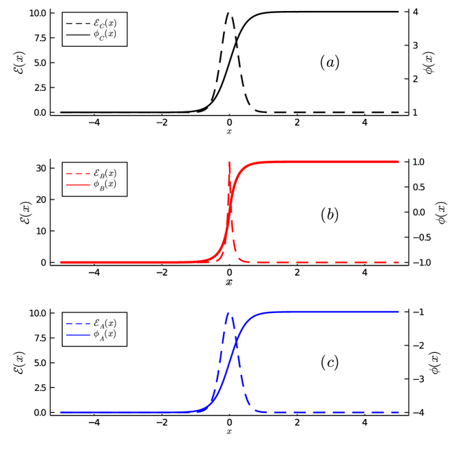
Figure 1: Field solutions (continuous lines) and energy densities (dashed lines) for the kinks $A$ (blue), $B$ (red) and $C$ (black). The parameters are selected as follows: $v_{1}=1,\,v_{2}=4,\lambda=1,\delta=0.$

Fig. (1) displays the plots for the three kink solutions and the corresponding energy densities. We observe that the profiles of the three field configurations display a characteristic kink behavior. The energy densities for $\phi_{A}(x)$ and $\phi_{C}(x)$ are smooth energy packets localised around the kink position, whereas the energy density for $\phi_{B}(x)$ presents a spike maxima because the second order derivative of $\phi_{B}(x)$ is discontinuous at the kink position.

We point out that we can define two parity symmetry operations $P_{x}$ and $P_{\phi}$ that invert the coordinate or field sign respectively: $P_{x}\phi(x)=\phi(-x)$ and $P_{\phi}\phi(x)=-\phi(x)$. The first symmetry transforms any kink into its corresponding anti-kink $P_{x}\phi_{K}(x)=\phi_{\bar{K}}(x)$. In the case of the $\phi_{B}(x)$ both symmetries coincide. However $P_{\phi}$ transforms the kink defined on $(-v_{2},-v_{1})$ sector into the anti-kink of the $(v_{1},v_{2})$ topological sector as follows

$$P_{\phi}\,\phi_{A}(x)=-\phi_{A}(x)=\phi_{\bar{C}}(x)\,,\qquad\qquad P_{\phi}\phi_{\bar{A}}(x)=\phi_{C}(x).$$ (18)

We call $P_{x}$ and $P_{\phi}$ the charge and mirror symmetries.

3.2 Kink solution for non degenerate minima ($\delta\neq 0$)

As the transition to the $\delta>0$ phase takes place the potential minima are no longer degenerate, $U(\pm V_{1})>U(\pm V_{2})=0$. There are now only two absolute minima, hence a unique kink interpolates between $\phi(-\infty)=-V_{2}$ to $\phi(\infty)=V_{2}$, as well as its corresponding anti-kink. To determine the kink configuration we substitute the potential Eq. (2.1) into Eq. (9) and perform the integrations in the intervals $(0,v_{2})$ and $(-v_{2},0)$ separately. In the entire interval $(0,v_{2})$ the field $\phi$ is positive, considering that $\phi_{m}=0$, and selecting the kink position at $x_{0}=0$ we find

$$x=\int^{\phi}_{0}\frac{d\phi}{\sqrt{2U(\phi)}}=\frac{1}{m_{2}}\log(\frac{(m_{2}/\sqrt{2}\lambda)\sqrt{(v_{1}-\phi)^{2}+\delta}+(\phi-v_{1})\Delta_{v}+\delta}{(v_{2}-\phi)})-g_{0},$$ (19)

where $\Delta_{v}=v_{2}-v_{1}$ and $g_{0}$ is defined as

$$g_{0}=\frac{1}{m_{2}}\log(\frac{(m_{2}/\sqrt{2}\lambda)\sqrt{v_{1}^{2}+\delta}-v_{1}\Delta_{v}+\delta}{v_{2}}).$$ (20)

An analogous expression is obtained for $x\leq 0$. Both relations can be explicitly inverted and the results are summarized in the following expression

$$\phi_{\delta}(x)=\text{sgn}(x)\left(\frac{v_{2}\,e^{2m_{2}(\absolutevalue{x}+g_{0})}+2(v_{2}v_{1}-v_{1}^{2}-\delta)\,e^{m_{2}(\absolutevalue{x}+g_{0})}-v_{2}\delta}{e^{2m_{2}(\absolutevalue{x}+g_{0})}+2\,\Delta_{v}\,e^{m_{2}(\absolutevalue{x}+g_{0})}-\delta}\right).$$ (21)

We can directly verify that $\phi_{\delta}(x)$ and its first derivative are continuous everywhere, but its second derivative is discontinuous at the origin ($\phi(0)=0$) in agreement with Eq. (2) and the discontinuity that $\partial U/\partial\phi$ presents at that point. The topological charge for $\phi_{\delta}$ is given as $Q_{\delta}=\pm 1$. The kink mass is evaluated using Eqs. (3,8) with the following result

$$M_{\delta} =\int_{-v_{2}}^{v_{2}}{\sqrt{2\lambda[(\absolutevalue{\phi}-v_{1})^{2}+\delta](\absolutevalue{\phi}-v_{2})^{2}}d\phi}$$ (22)

$$=\frac{\sqrt{2\lambda}}{3}\Bigg{[}\sqrt{\Delta_{v}^{2}+\delta}(\Delta_{v}^{2}-2\delta)-\,\left(v_{1}(v_{1}-3v_{2})-2\delta\right)\,\sqrt{v_{1}^{2}+\delta}$$

$$\qquad+\,3\,\delta\Delta_{v}\log(\frac{\sqrt{\Delta_{v}^{2}+\delta}+\Delta_{v}}{\sqrt{v_{1}^{2}+\delta}-v_{1}})\Bigg{]}.$$

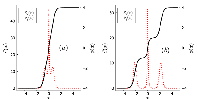
Figure 2: Field solutions $\phi_{\delta}(x)$ (continuous lines) and their corresponding energy densities (dashed lines) for two values of the control parameter: $\delta=0.5$ (left plot) and $\delta=0.001$ (right plot). The value of the other parameters are $v_{1}=1,\,v_{2}=4,\lambda=1$.

Fig.(2) displays plots of $\phi_{\delta}(x)$ and the energy density ${\cal E}_{\delta}(x)$ for two values of the $\delta$ parameter. For small $\delta$, $\phi_{\delta}(x)$ clearly shows three successive kinks with values in the regions: $(-v_{2},-v_{1}),\,(-v_{1},v_{1}),(v_{1},v_{2})$. These kinks are centered at the positions $x=-x_{m},\,x=0,\,x=x_{m}$. The central position $(x=0)$ is arbitrarily selected because of the translational invariance symmetry of the system; however $x_{m}$ is fixed and its value will be explained below. At the positions of each of the internal kinks the energy density shows a lump-like distribution, and in particular the central energy packet presents a spike configuration. Based on these results we conclude that $\phi_{\delta}$ is a bound state resulting from the merge of the $\phi_{A}$, $\phi_{B}$ and $\phi_{C}$ kinks. To support this claim we notice that the following charge equality is trivially fulfilled

$$Q_{\delta}\,=\,Q_{A}\,+\,Q_{B}\,+\,Q_{C}=1.$$ (23)

Additionally, it follows that for small values of $\delta$ the kink mass in Eq. (22) can be approximated as

$$M_{\delta}\approx M_{A}\,+\,M_{B}\,+\,M_{C}+m\,\delta\,\left(\frac{|Q_{B}|}{1-|Q_{B}|}+\log\left[\frac{2\,m^{2}\,|Q_{B}|}{\lambda\,\delta(1-|Q_{B}|)}\right]\right)+{\cal O}(\delta^{2})$$ (24)

where we used the values for $M_{A}=M_{C}$ Eq. (13) and $M_{B}$ Eq. (17). The mass of the $\phi_{\delta}$ kink results from the addition of the masses of the constituent kinks and a term that, as shown in section (4), represents the potential energy of the system evaluated at the equilibrium configuration Eq. (24).

Using Eq. (19) evaluated at $x=x_{m}$ and $\phi=V_{m}$ we obtain the value of $x_{m}$ that determines the distance of $\phi_{A}$ and $\phi_{C}$ relative to $\phi_{B}$. For small $\delta$ it is approximated as

$$x_{m}\approx\frac{1}{m}\,\log\left(\frac{2\,|Q_{1}|m^{2}}{\lambda\,\delta}\right)\,,\qquad\qquad\delta<<\frac{m^{2}}{\lambda}.$$ (25)

Hence $\phi_{\delta}$ is a multi-kink state $\phi_{\delta}(x)\approx\phi_{A}(x+x_{m})+\phi_{B}(x)+\phi_{C}(x-x_{m})$, where according to Eq. (25) there is a large but finite separation. In section 4 we shall prove that $\pm x_{m}$ represent the equilibrium positions of the forces that act on $\phi_{A}$ and $\phi_{C}$, considering that $\phi_{B}$ is fixed at $x=0$.

A fundamental property of solitary waves is that they are non-dispersive, namely they represent localised energy packages that move with constant speed, maintaining their initial structure. To verify that the previously obtained solutions can be considered as true solitary waves, we apply a boost by defining $\phi_{X}(\gamma(x-vt))$, with $\gamma=1/\sqrt{(1-v^{2})}$ where $\phi_{X}$ is any of the kink solutions Eqs. (11, 15,21). We confim that $\phi_{X}(\xi)$ is a solution of the time dependent Eq. (2), hence the four kinks ($\phi_{A},\,\phi_{B},\,\phi_{C},\,\phi_{\delta}$) and their corresponding anti-kinks are indeed solitary waves.

4 Kink interactions

In this section we analyse the effect of combining two kinks or a kink with an anti-kink, and compute the forces that act between them. In general these configurations will be time dependent, but if we consider a $KK$ or $K{\bar{K}}$ pair that at an initial time is separated by a large distance $R>>1/m$, for a short period it will experiment a rigid displacement and the force can be determined. In order to have a continuous finite energy configuration it is required that a kink $K$ is followed by an antinkink ${\bar{K}}$ defined in the same topological sector or a kink $K^{\prime}$ defined in a contiguous topological sector. Thus we consider three independent configurations: $C{\bar{C}}$, $B{\bar{B}}$ and $BC$ that will give rise to different expressions for the corresponding forces. These results will be extended to analyse the forces that act within the multi-kink $\phi_{\delta}$,

The momentum density for a scalar field obtained from Noether’s theorem is given as $-\left(\frac{\partial\phi}{\partial t}\right)\left(\frac{\partial\phi}{\partial x}\right)$. Integrating this expression in the interval $(X,\infty)$ and utilising Eq. (8) the force acting on the field to the right of $X$ is obtained as Manton and Sutcliffe (2004); Manton (2019)

$$F=\frac{dP}{dt}=-\frac{d}{dt}\int_{X}^{\infty}\left(\frac{\partial\phi}{\partial t}\right)\left(\frac{\partial\phi}{\partial x}\right)dx=\left[\frac{1}{2}\left(\frac{d\phi}{dx}\right)^{2}-U(\phi)\right]_{x=X}.$$ (26)

Here we took into account that the last two terms in the previous equation cancel out as $x\to\infty$.

4.1 $\delta=0$ case

First we analyse the $C{\bar{C}}$ configuration in which the kink $C$ localised at $x=-q$ occupies the $x<0$ region, whereas ${\bar{C}}$ defined for $x>0$ is situated at $x=q$; the ansatz for the $C{\bar{C}}$ field is represented as $\phi_{C{\bar{C}}}(x)=\phi_{C}(x+q)+\phi_{\bar{C}}(x-q)-v_{2}$. When $q\gg 1/m$ we can approximate $\phi_{\bar{C}}(x-q)-v_{2}\approx 0$ for $x<0$, and $\phi_{C}(x+q)-v_{2}\approx 0$ on the positive $x$-axis; hence $\phi_{C{\bar{C}}}$ is a correct representation for the $C{\bar{C}}$ system as shown in Fig.(3). Thus, if we select $X=0$ in Eq. (26) $F$ represents the force exerted on ${\bar{C}}$. Selecting $x<<q$ and $q\gg 1/m$ we obtain $\phi_{C{\bar{C}}}(x)\approx v_{2}+2(v_{1}-v_{2})\,e^{-mq}+{\cal O}(x^{2})$, plugging this expression into Eq. (26) yields $\left(\frac{d\phi_{A{\bar{A}}}}{dx}\right)^{2}_{x=0}=0$ and $U_{0}(\phi_{A{\bar{A}}})_{x=0}=\frac{m^{4}}{\lambda}e^{-2mq}$, that results in an attractive interaction with an exponential decay given as follows

$$F_{C{\bar{C}}}\approx-\frac{m^{4}}{\lambda}\,e^{-m\,R},$$ (27)

where $R=2q$ is the separation between the kink and the anti-kink.

In order to compute $F_{B{\bar{B}}}$ we define $\phi_{B{\bar{B}}}(x)=\phi_{B}(x+q)+\phi_{\bar{B}}(x-q)-v_{1}$. Using $\phi_{B}(x)$ given in Eq. (15), the following asymptotic expression $(x<<1\,,\,q\gg 1/m)$ follows up $\phi_{B{\bar{B}}}(x)\approx-v_{1}+2\frac{v_{1}}{v_{2}}(v_{2}-v_{1})\,e^{-mq}+{\cal O}(x^{2})$, from which we obtain $\left(\frac{d\phi_{B{\bar{B}}}}{dx}\right)^{2}_{x=0}=0$ and $U_{0}(\phi_{B{\bar{B}}})_{x=0}=(\frac{v_{1}}{v_{2}})^{2}\frac{m^{4}}{\lambda}e^{-mR}$, that also produce an attractive interaction but with different strength

$$F_{B{\bar{B}}}=-Q_{B}^{2}\,\frac{m^{4}}{\lambda}\,e^{-m\,R}.$$ (28)

We now turn the attention to the $BC$ system. The field ansatz configuration is written as $\phi_{B{C}}(x)=\phi_{B}(x+q)+\phi_{C}(x-q)-v_{1}$, Fig.(3) shows that $\phi_{B{C}}(x)$ represents a field that interpolates between the $-v_{1}$ and the $+v_{2}$ potential minima. When $x<<1\,,\,q\gg 1/m$ the asymptotic expression for $\phi_{B{C}}(x)$ reduces to

$$\phi_{B{C}}(x)\approx-v_{1}+\frac{(v_{2}-v_{1})^{2}}{v_{2}}\,e^{-mq}+m\,x\,\frac{(v_{2}^{2}-v_{1}^{2})}{v_{2}}\,e^{-mq}+{\cal O}(x^{2}).$$ (29)

In this case we find $\frac{1}{2}\left(\frac{d\phi_{Bc}}{dx}\right)^{2}_{x=0}=(1+\frac{v_{1}}{v_{2}})^{2}\frac{m^{4}}{4\lambda}e^{-mR}$ and $U_{0}(\phi_{BC})_{x=0}=(1-\frac{v_{1}}{v_{2}})^{2}\frac{m^{4}}{4\lambda}e^{-mR}$; that lead to a repulsive interaction

$$F_{BC}=\absolutevalue{Q_{B}}\frac{m^{4}}{\lambda}\,e^{-m\,R}.$$ (30)

The previous results show that generically the kink-anti-kink interaction is attractive, while the kink-kink interaction is repulsive, and that in both cases the interaction decays exponentially as the kink separation increases. However the interaction strengths are not equal in absolute value, but rather the ratio of the forces are given as follows

$$\absolutevalue{\frac{F_{B{\bar{B}}}}{F_{BC}}}=\absolutevalue{Q_{B}},\qquad\qquad\absolutevalue{\frac{F_{C{\bar{C}}}}{F_{BC}}}=\frac{1}{\absolutevalue{Q_{B}}}.$$ (31)

The forces for other multi-kink configurations can be obtained from the relations $F_{A{\bar{A}}}=F_{C{\bar{C}}}$, $F_{AB}=F_{BC}$.

4.2 $\delta>0$ case

When $\delta>0$, $\phi_{A}$, $\phi_{B}$ and $\phi_{C}$ are no longer exact solutions of Eq. (8), instead we have a new kink $\phi_{\delta}$ that interpolates between the two absolute potential minima $\pm v_{2}$. However, as mentioned in section (3), the $\phi_{\delta}(x)$ profile resembles a multi-kink formed from the merge of $\phi_{A}$, $\phi_{B}$ and $\phi_{C}$, which leads us to analyse the configuration defined by the following ansatz

$$\phi_{ABC}(x;q)=\phi_{A}(x+q)+\phi_{B}(x)+\phi_{C}(x-q).$$ (32)

We compute the pair interactions between the components of $\phi_{ABC}(x;q)$ and determine if it is possible to find a value of $q$ for which the configuration is stable. The force exerted on the field $\phi_{C}(x-q)$ in Eq. (32) is dominated from the $\phi_{B}-\phi_{C}$ interaction, that was already calculated in Eq. (30). However that calculation was carried out for $\delta=0$, which only includes the potential $U_{0}(\phi)$ in Eq. (2.1). Hence we must add the contribution from $\Delta U(\phi)=\lambda\delta\left(\absolutevalue{\phi}-v_{2}\right)^{2}$ evaluated at $\phi_{BC}(0)$ using Eq. (29). A direct calculation yields $\Delta U(\phi_{BC}(0))\approx m^{2}\delta/2$. Adding this result to $F_{BC}$ given in Eq. (30) the total force acting on $\phi_{C}$ results in

$$F_{AB;C}=\absolutevalue{Q_{B}}\frac{m^{4}}{\lambda}\,e^{-m\,q}-\frac{m^{2}}{2}\delta.$$ (33)

Remarkably, in addition to the repulsive contribution, there is an attractive constant long range force. Thus, the dynamics of the position of the kink $\phi_{C}$ takes place in an effective potential $V_{AB;C}(q)$ that is obtained from the space integral of Eq. (33) leading to

$$V_{AB;C}(q)=\absolutevalue{Q_{B}}\frac{m^{3}}{\lambda}\,e^{-m\,q}+\frac{m^{2}}{2}\delta\,+\frac{1}{2}K.$$ (34)

where $K$ is a constant. This potential has a stable equilibrium point $q=x_{m}$, that coincides with the separation between the contiguous kinks components of $\phi_{\delta}$ given in Eq. (25). As the force acting on $\phi_{A}$ is identical to Eq. (33) and the the force on $\phi_{B}$ cancels, it follows that the effective potential for the $\phi_{ABC}$ multikink is $V_{ABC}(q)=2V_{AB;C}(q)$. When this potential is evaluated at the equilibrium point $q=x_{m}$ and selecting the constant in Eq. (34) as $K=m\delta\left(\frac{2|Q_{B}|-1}{1-|Q_{B}|}-\log(1-|Q_{B}|)\right)$ it follows that $V_{ABC}(x_{m})$ exactly coincides with the correction of order $\delta$ to the $\phi_{\delta}$ mass in Eq. (24), confirming that it represents the potential energy of the multi-kink at the equilibrium configuration.

Finally, to complete the interpretation of $\phi_{\delta}$ as a $\phi_{A}\,+\phi_{B}\,+\phi_{C}$ multi-kink state, we notice that for $\delta<<1$, both $\phi_{\delta}(x)$ Eq. (21) and $\phi_{ABC}(x;x_{m})$ Eq. (32) reduce to the same expression

$$\phi_{\delta}(x)=\text{sgn}(x)\left(\frac{4\,v_{2}\,\Delta_{v}^{2}\,e^{2m(\text{sgn}(x)-x_{m})}\,+\,4\,v_{1}\,\Delta_{v}^{2}\,e^{m(\text{sgn}(x)-x_{m})}\,-\,v_{2}\,\delta}{4\,\Delta_{v}^{2}\,e^{2m(\text{sgn}(x)-x_{m})}\,+\,4\,\Delta_{v}^{2}\,e^{m(\text{sgn}(x)-x_{m})}-\delta}\right),$$ (35)

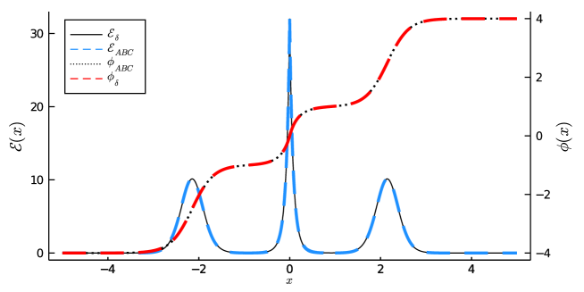
Figure 4: Comparison of the exact field configuration $\phi_{\delta}(x)$ Eq. (21) dotted (black) line, with the multi-kink $\phi_{A}(x+x_{m})+\phi_{B}(x)+\phi_{C}(x-x_{m})$ Eq. (35) dashed (red) line, where $x_{m}$ is given in Eq. (25). The corresponding energy densities are also compared. As observed the two configurations coincide for small $\delta$. The parameter values are $\delta=0.001,\,v_{1}=1,\,v_{2}=4,\lambda=1$.

where $\Delta_{v}=v_{2}-v_{1}$. Fig.(4) compares the plots obtained from the previous expression with the exact solution given in Eq. (21). It is clearly shown that the difference between the two expressions becomes imperceptible as the $\delta$ parameter decreases.

5 Quantum mass corrections, and renormalization

We now turn our attention to the study of field excitations around the kink configurations. The kinks are expected to be stable, this is verified by showing that the spectrum of the fluctuations is positive defined. Furthermore the use of a WKB approximation enables computing the quantum corrections to the kink mass. In what follows we mainly focus on the case of degenerate potential minima $\delta=0$, hence the field potential is given by $U_{0}(\phi)$ in Eq. (2.1).

The field $\phi(x,t)$ is written as the sum of the classical kink solution $\phi_{K}(x)$ and a small fluctuation $\eta(x,t)$ as follows $\phi(x,t)=\phi_{K}(x)+\eta(x,t)$. If we substitute the previous decomposition into the energy functional Eq. (3), integrating by parts and taking into account that $\phi_{K}(x)$ satisfy Eq. (8), we find that

$$E_{K}=M_{K}\,+\int_{-\infty}^{\infty}dx\left\{\frac{1}{2}\left(\frac{d\eta}{dt}\right)^{2}+\eta\left(-\frac{d^{2}\eta}{dx^{2}}+U_{0}^{\prime\prime}(\phi_{K})\eta+\delta(x-x_{c})\,disc\,\partial_{x}\eta\,\right)+{\cal O}(\eta^{3})\right\}.$$ (36)

Compared with the usual results Rajaraman (1982); Dashen et al. (1974); Goldstone and Jackiw (1975); Boya and Casahorran (1989), this expression includes an extra term that takes into account that $\partial\eta/\partial x$ is discontinuous at the point $x_{c}$ where $\phi_{K}(x_{c})=0$. In Eq. (36) $disc\,\partial_{x}\eta$ is given by

$$disc\,\partial_{x}\eta=\lim_{\epsilon\to 0}\left\{\left(\frac{\partial\eta}{\partial x}\right)_{x_{c}+\epsilon}-\left(\frac{\partial\eta}{\partial x}\right)_{x_{c}-\epsilon}\right\}.$$ (37)

Taking the usual expansion $\eta(x,t)=\sum_{m}\eta_{m}(x)\,e^{i\omega_{m}t}$, the energy in Eq. (36) is diagonalised if the functions $\eta_{m}(x)$ are selected as eigenfunctions of the following one dimensional Schrödinger equation

$$\left(-\frac{d^{2}}{dx^{2}}+U^{\prime\prime}(\phi_{K})+D_{m}\,\delta(x-x_{c})\right)\,\eta_{m}(x)=\omega_{m}^{2}\,\eta_{m}(x),$$ (38)

where $D_{m}=disc\,\partial_{x}\eta_{m}/\eta_{m}(x_{c})$. The fact that $U_{0}(\phi)$ in (2.1) is a quadratic form permits making contact with the supersymmetric quantum mechanics formalism Boya and Casahorran (1989); Cooper et al. (1995). Writing $U_{0}(\phi)=\frac{1}{2}V(\phi)^{2}$ with $V(\phi)=\sqrt{2\lambda}\left(\absolutevalue{\phi}-v_{1}\right)\left(\absolutevalue{\phi}-v_{2}\right)$ results in the superpotential $W(\phi)$ and the SUSY-QM potentials $V^{\pm}_{S}(x)$ being expressed as follows

$$W(x)=\frac{\partial V}{\partial\phi}[\phi_{K}(x)],\qquad\qquad V^{\pm}_{S}(x)=W^{2}(x)\mp\frac{dW(x)}{dx}.$$ (39)

The potential in the stability Eq. (38) coincides with one of the SUSY-QM potentials $U_{0}^{\prime\prime}(\phi_{K})=V^{+}_{S}(x)$.

The solutions of Eq. (38) apply both (i) when the fluctuations take place around the vacuum configurations $\phi_{V}=\pm V_{1,2}$, in which case $U^{\prime\prime}(V_{1,2}))=m$ and the solution is given by $\omega_{{k^{\prime}}}^{2}=m^{2}+k^{\prime\,2}$ and $\eta_{k^{\prime}}(x)=e^{i{k^{\prime}}x}$; and (ii) when the background is the kink configuration, the explicit solutions of which will be presented in following paragraphs, but generically include a discrete $\omega_{n}$ and a continuous $\omega_{k}$ spectrum whose eigenfunctions have an asymptotic behavior $\eta_{k}(x)=e^{ikx\pm\delta(k)/2}$ as $x\to\pm\infty$, where $\delta(k)$ is the phase shift. Notice that the asymptotic behavior of $\eta_{k}(x)$ implies a reflectionless potential.

The contribution of the continuous modes is computed incorporating a regularization scheme in which the system is enclosed in a finite box of length $L$. Hence the kink excitation spectrum $\omega_{j}^{2}=m^{2}+k_{j}^{2}$, and that of the vacuum fluctuations $\omega_{j}^{\prime\,2}=+m^{2}+k_{j}^{\prime\,2}$ becomes discrete. Taking into account the periodic boundary conditions, $Lk_{j}+\delta(k_{j})=Lk_{j}^{\prime}=2\,\pi\,j$, we calculate the zero point energy contribution to the kink mass, subtracting the vacuum energy, to obtain

$$M_{cont}=\frac{1}{2}\sum_{j}\left(\sqrt{m^{2}+k_{j}^{2})}-\sqrt{m^{2}+k_{j}^{\prime\,2}}\right)\sim-\frac{1}{2}\sum_{j}\frac{1}{L}\delta(k_{j})\frac{\Delta\omega_{j}}{\Delta k_{j}}\sim-\int_{-\infty}^{\infty}\frac{dk}{4\pi}\frac{d\omega_{k}}{dk}\delta(k),$$ (40)

where in the last equality we set $\frac{1}{L}\sum_{j}\to\frac{dk}{2\pi}$ as ${L\to\infty}$. This quantity is still logarithmically divergent and it requires the addition of a mass counter-term obtained by a one loop perturbative renormalization scheme Dashen et al. (1974); Aguirre and Flores-Hidalgo (2020). The mass counter-term takes the form $-\,\frac{1}{2}\,\delta\,m^{2}\,\langle{\cal V}\rangle$, where the tadpole contribution and the average stability potential are given as

$$\delta m^{2} =\,\frac{6\lambda}{\pi}\,\int_{0}^{\Lambda}\,\frac{dk}{\left(k^{2}+m^{2}\right)^{1/2}}\,=\,\frac{6\lambda}{\pi}\,\log\frac{2\Lambda}{m},$$

$$\langle{\cal V}\rangle =\frac{1}{12\lambda}\,\int_{-\infty}^{\infty}\,dx\,{\cal V}(x),\qquad{\cal V}(x)=U^{\prime\prime}(\phi_{K}(x))-m^{2}.$$ (41)

Here $\Lambda$ is the momentum cut-off. Gathering the contributions of the classical kink mass $M_{K}$, the discrete as well as the continuous zero energy modes, including the subtraction of the vacuum energy Eq. (40), together with the kink renormalization term Eq. (5), we finally arrive to the following expression for the quantum kink mass

$$\tilde{M}_{K}=M_{K}\,+\sum_{n}\,\frac{1}{2}\,\omega_{n}-\int_{0}^{\Lambda}\,\frac{dk}{2\pi}\,\delta(k)\frac{d\omega_{k}}{dk}-\,\frac{1}{2}\,\delta\,m^{2}\,\langle{\cal V}\rangle.$$ (42)

In the next subsections we demonstrate that the formalism gives finite results for the quantum masses of the $\phi_{A}$, $\phi_{B}$ and $\phi_{C}$ kinks.

5.1 $\phi_{C}$ quantum mass corrections

In this subsection we compute the quantum mass $\tilde{M}_{C}$ for the kink $\phi_{C}$. Using the expression for $\phi_{C}(x)$ to evaluate the effective potential in Eq. (38), and taking into account that $\phi_{C}(x)$ is positive in the complete $x\in(-\infty,\infty)$ interval, it follows that equation Eq. (38) becomes

$$\left(-\,\frac{1}{2}\,\frac{d^{2}\eta_{k}}{dz^{2}}+{\cal V}_{C}(z)\right)\eta_{k}\, =\epsilon_{k}\,\eta_{k}\,,$$

$${\cal V}_{C}(z)=U_{0}^{\prime\prime}(\phi_{C}(z))-m^{2}\, =\,-3\,m^{2}\,\sech^{2}\left(z\right)\,,$$ (43)

where $z=mx/2$ and $\epsilon_{k}=2(\omega_{k}^{2}-m^{2})/m^{2}$. Eq. (5.1) is one of the SUSY partner equations in (39) with the superpotential $W(z)=m\tanh(z)$. The solutions to Eq. (5.1) are well known Morse and H. (1953). The spectrum consists of two discrete levels with energies and eigenfunctions given by: $\omega^{2}_{0}=0$, $\eta_{0}(x)=\sech^{2}\left(z\right)$; and $\omega^{2}_{1}=\frac{3}{4}m^{2}$, $\eta_{1}(x)=\tanh\left(z\right)\,\sech\left(z\right)$. The continuous spectrum $\omega^{2}_{k}=k^{2}+m^{2}$ has the eigenfunctions $\eta_{k}(x)=\,e^{ikx}\,H(\tanh z)$ where the function $H(\xi)$ is defined as

$$H(\xi)=\left(m^{2}(3\xi^{2}-1)-4k^{2}-\,i\,6\,k\,m\,\xi\right).$$ (44)

The asymptotic behavior of the continuous wave functions takes the following form $\eta_{k}(x)=e^{ikx\pm\delta_{C}(k)/2}$, where $\delta_{C}(k)=-2\arctan 3km/(m^{2}-k^{2})$. Plugging $\delta_{C}(k)$ into Eq. (40), integrating by parts, and separating the finite contribution from the one that diverge with $\Lambda$, leads to

$$M_{cont-C}=-\frac{3m}{2\pi}-\frac{6m}{2\pi}\int_{0}^{\Lambda}\,dk\,\frac{(m^{2}+2k^{2})}{(m^{2}+4k^{2})\,\sqrt{m^{2}+k^{2}}}\,=-\frac{m}{2\pi}\left(3+\frac{\pi}{\sqrt{3}}+3\log\frac{2\Lambda}{m}\right).$$ (45)

This quantity is still logarithmically divergent and we have to add the mass counter-term indicated in Eqs. (5,42). Taking into account that $\langle{\cal V_{C}}\rangle=-m/2\lambda$, the mass counter-term reduces to

$$-\,\frac{1}{2}\,\delta\,m^{2}\,\langle{\cal V_{C}}\rangle\,=\frac{3}{2\pi}\,m\,\log\frac{2\Lambda}{m},$$ (46)

which exactly cancels the divergent term in Eq. (45). It is now straightforward to add the contributions in Eqs. (45,46) with the classical kink mass and the discrete energy $\frac{1}{2}\omega_{1}$, to obtain the final result for the quantum $\phi_{C}$ kink mass

$${\tilde{M}}_{C}=\frac{m^{3}}{12\lambda}+m\,\left(\frac{1}{4\sqrt{3}}-\frac{3}{2\pi}\right)\,+\,{\cal O}(\lambda).$$ (47)

The same result is obtained for the $A$ kink ${\tilde{M}}_{A}={\tilde{M}}_{C}$.

It is noteworthy that the stability equation (5.1), its solutions, and the quantum mass (47) for the $\phi_{C}$ kink, coincide with the results previously obtained for the $\phi^{4}$ model Dashen et al. (1974), notwithstanding the $\phi^{4}$ and $\phi^{4}_{G}$ models are notoriously different. This can be explained by the reconstruction method Jackiw (1977); Vachaspati (2004), in which the structure of the scalar field theory is obtained from the stability equations and the knowledge of the bound spectrum. In particular it has been show that when the spectrum has two bound states, the reconstruction is not unique Bazeia and Bemfica (2017). Hence we conclude that considering the stability equation and its corresponding spectrum, the application of the reconstruction method should produce both the $\phi^{4}$ and $\phi^{4}_{G}$ models.

5.2 $\phi_{B}$ quantum mass corrections

Consider now the quantum fluctuations around the $\phi_{B}$ kink. In Eq. (15) we recall that $\phi_{B}(x)$ is separately defined in the positive and negative $x$-axis. Using the expression for $\phi_{B}(x)$ to evaluate the effective potential in Eq. (38) leads to the following Schrödinger equation

$$\left(-\frac{1}{2}\,\frac{d^{2}}{dy^{2}}+\,3\,\csch^{2}\left(y\right)+\frac{D_{k}}{m^{2}}\,\delta(x-x_{c})\right)\eta_{k}(y)=\epsilon_{k}\,\eta_{k}(y),$$ (48)

where $y=\frac{mx}{2}+\frac{1}{2}sgn(x)\log\frac{v_{2}}{v_{1}}$ was piecewise defined in Eq. (14), $\epsilon_{k}=2(\omega_{k}^{2}-m^{2})/m^{2}$, and the effective potential Eq. (5) is now given as ${\cal V}_{B}(z)=U_{0}^{\prime\prime}(\phi_{B}(z))-m^{2}\,=\,3\,m^{2}\csch^{2}\left(y\right)$. Note that according to Eqs. (37,38) the delta term potential has to be included because $\phi_{B}(x)$ cancels at $x=0$, so the derivative of $\eta_{k}$ is expected to be discontinuous at the origin. Eq. (48) is one of the SUSY-QM equation corresponding to the superpotential $W(y)=m\coth y$.

We present the details of the solutions to Eq. (48) in the appendix B. The spectrum and its corresponding eigenfunctions are given as

$$\omega^{2}_{0} =0\,,\qquad\qquad\qquad\,\,\,\,\,\eta_{0}(x)=\csch^{2}\left(y\right)\,,$$

$$\omega^{2}_{1} =\frac{3}{4}m^{2}\,,\qquad\qquad\,\,\,\,\,\,\,\,\eta_{1}(x)=\coth\left(y\right)\,\csch\left(y\right),$$

$$\omega^{2}_{k} =k^{2}+m^{2}\,,\qquad\qquad\eta_{k}(x)=e^{ikx}\,H(\coth y)/H(\text{sgn}(x)\,C_{v}).$$ (49)

where $C_{v}=\coth\left(\frac{1}{2}\log\frac{v_{2}}{v_{1}}\right)=(v_{1}+v_{2})/(v_{2}-v_{1})$ and the function $H(y)$ is defined in Eq. (44). The spectrum coincides with that calculated in the previous subsection, but the eigenfunctions are now given in terms of $\coth y$ instead of $\tanh x$ functions. All the eigenfunctions in Eq. (5.2) are continuous at the origin, but their first derivatives are discontinuous. In particular, as expected, the zero energy mode is given by $\eta_{0}(y)\propto d\phi_{B}/dx(y)$, with $disc\eta_{x,0}=-2m^{2}v_{1}v_{2}(v_{1}+v_{2})/(v_{2}-v_{1})^{2}$. For the two discrete modes the values of the coefficients $D_{k}$ in Eq. (48) are negative, thus the delta terms represent attractive potentials that explain the existence of bound states.

For the continuous states, we observe that the potential in Eq. (48) is again transparent, hence $\eta_{k}(x)=e^{ikx\pm\delta_{B}(k)/2}$ as $x\to\pm\infty$, and the phase shift computed from Eq. (5.2) becomes

$$\delta_{B}(k)=-2\arctan\left[\frac{3\,k\,m}{m^{2}-k^{2}}\right]+2\arctan\left[\frac{6\,k\,m\,C_{v}}{m^{2}(3C_{v}^{2}-1)-4k^{2}}\right].$$ (50)

The first part of $\delta_{B}(k)$ exactly coincides with the phase shift $\delta_{C}(k)$ obtained in the previous subsection. Hence we can separate the contribution of the continuos modes to the kink energy in Eq. (40) as $M_{cont-B}=M_{cont-C}+\Delta M_{cont-B}$, where $M_{cont-C}$ is given in Eq. (45) and $\Delta M_{cont-B}$ is obtained substituting the second part of Eq. (50) into Eq. (40) and integrating by parts resulting in

$$\Delta M_{cont-B}=\frac{3m}{2\pi}C_{v}+\frac{3mC_{v}}{\pi}\int_{0}^{\Lambda}\frac{\omega_{k}\,[m^{2}(3C_{v}^{2}-1)+4k^{2}]}{\left[m^{2}(3C_{v}^{2}-1)-4k^{2}\right]^{2}+9k^{2}m^{2}C_{v}^{2}}\,\,dk,$$ (51)

where $\omega_{k}=\sqrt{m^{2}+k^{2}}$. The denominator in the preceding integral can be factorized according to $4(k^{2}-m^{2}r_{1})(k^{2}-m^{2}r_{2})$, where

$$r_{1,2}=\frac{1}{8}(3C_{v}^{2}+2)\pm\frac{3}{8}\sqrt{4-3C_{v}^{2}}.$$ (52)

The integral in Eq. (51) can now be explicitly evaluated separating the denominator in partial fractions. After a detailed calculation the final result for $\Delta M_{cont-B}$ can be worked out as

$$\Delta M_{cont-B}=\frac{3m}{2\pi}C_{v}\Bigg{[}1+F(r_{1},r_{2})+\log\frac{2\Lambda}{m}\Bigg{]},$$ (53)

where $F(r_{1},r_{2})$ is defined as

$$F(r_{1},r_{2}) =\frac{1}{2(r_{1}-r_{2})}\Bigg{[}\left(4r_{2}+3C_{v}^{2}-1\right)G(r_{2})-\left(4r_{1}+3C_{v}^{2}-1\right)G(r_{1})\Bigg{]},$$

$$G(r_{i}) =\sqrt{\frac{1+r_{i}}{r_{i}}}\,\operatorname{arctanh}\sqrt{\frac{1+r_{i}}{r_{i}}},\qquad i=1,2.$$ (54)

Considering that $\langle{\cal V_{C}}\rangle=mv_{1}/\lambda(v_{2}-v_{1})$, the mass counter-term is worked out as

$$-\,\frac{1}{2}\,\delta m^{2}\,\langle{\cal V_{B}}\rangle\,=-\frac{3\,m}{\pi}\,\frac{v_{1}}{v_{2}-v_{1}}\,\log\frac{2\Lambda}{m}.$$ (55)

Adding the contributions of the continuous modes in Eqs. (45,53) to the previous result corroborates the exact cancelation of the divergent terms. Collecting all the finite terms yields the quantum mass for the $\phi_{B}$ kink

$${\tilde{M}}_{B}=\frac{m^{3}}{6\,\lambda}\frac{Q_{B}^{2}(3-\absolutevalue{Q_{B}})}{(1-\absolutevalue{Q_{B}})^{3}}+m\,\left(\frac{1}{4\sqrt{3}}\,+\frac{3}{\pi}\frac{v_{1}}{v_{2}-v_{1}}+\frac{3}{2\pi}\,C_{v}\,F(r_{1},r_{2})\right)+\,{\cal O}(\lambda).$$ (56)

This proves that the current formalism allows us to adequately analyse the discontinuities that appear in the case of kink B, giving rise to a finite value for the quantum mass of the kink.

Unlike the results obtained in the previous subsection, the stability equation and the quantum mass corrections of the $\phi_{B}$ kink Eqs. (48,5.2,56) have not been previously obtained. As mentioned, the use of the reconstruction method applied to the $\phi_{C}$ kink leads to either the $\phi^{4}$ or the $\phi^{4}_{G}$ models. However, we propose that a simultaneous application of the reconstruction formalism to the $\phi_{C}$ and $\phi_{B}$ solutions will probably lead to a unique $\phi^{4}_{G}$ field scalar theory, which is a topic that deserves further investigation.

6 Final considerations

This paper analyses the properties of the $\phi^{4}_{G}$ model. In spite of the non-analytical behavior of the potential, we prove that a systematic treatment of the discontinuities induced in the field configuration enables obtaining results with clear physical content. Kink solutions with well defined properties are obtained, and their mutual interactions as well as their quantum mass corrections are explicitly calculated. These results are of value for the study of scalar field theories in the presence of abrupt interfaces as well as for the study of non-equilibrium stationary steady-states Aron and Kulkarni (2020).

At the transition point $\delta=0$, where all the potential minima are degenerate, three kinks $\phi_{A}$, $\phi_{B}$, $\phi_{C}$ were found. The solutions $\phi_{A}(x)$ and $\phi_{C}(x)$ Eq. (11), are equivalent to those obtained for the kink in the $\phi^{4}$ model, but for $\phi_{B}$ it is essential to consider the effects of the potential discontinuities to obtain a novel solution and compute its quantum kink mass corrections (Eqs. 15 and 56).

The existence of multi-soliton solutions Gardner et al. (1967); Hirota (1971); Ablowitz et al. (1973) is of great interest to the understanding of the emergence of coherent structures Scott (2003); Ahlqvist and Greene (2015). Diverse mathematical techniques have been developed to obtain such solutions Arshad et al. (2017a, b); Hossen et al. (2018); Ullah et al. (2020). It should be noted that in general these solutions are time dependent. In this paper it is proven that a stationary multi-kink occurs near the transition from the degenerate to the non-degenerate potential phase. In this region, each of the $\phi_{A}(x)$, $\phi_{B}(x)$ and $\phi_{C}(x)$ kinks will be separately unstable, but they merge in a single stable multi-kink configuration because the mutual interactions produces a confining potential. This result was obtained in the context of the model $\phi^{4}_{G}$, but its appearance can be expected in general near a phase transition between a degenerate to a non-degenerate minima potential as long as in the transition point the potential possesses at least three absolute degenerate minima Demirkaya et al. (2017).

The analysis of the stability condition and the quantum corrections to the kink masses produced a modified Schrödinger equation, with a reflectionless potential that also includes an extra delta potential term. The study of the SUSY-QM structure Boya and Casahorran (1989); Cooper et al. (1995) of this equation, in which the superpotential $W(y)=m\coth y$ is defined in terms of a piecewise variable, clearly deserves further study. Similarly, the relation of the $\phi^{4}$ and $\phi^{4}_{G}$ through its connection to the reconstruction method Bazeia and Bemfica (2017) should also be subject to further investigation.

Appendix A Spontaneous symmetry breaking in the generalized $\phi^{4}_{G}$ theory

The generalized $\phi^{4}_{G}$ potential $U(\phi)$ in Eq. (2.1) has two different minima: $V_{1}$ and $V_{2}$, and each one is degenerate due to the $Z_{2}$ discrete symmetry of the theory. As a consequence, the spontaneous symmetry breaking of the theory can be induced by expanding the field $\phi$ around any of the non-equivalent minima $V_{i}\,,\,i=1,2$; yielding two independent Lagrangians $\mathcal{L}_{i}$. Substituting the expansion of the scalar field as $\phi(x)=V_{i}+\sigma_{i}(x)$ into Eq. (1) gives $\mathcal{L}_{i}$ as

$$\mathcal{L}_{i}=\frac{1}{2}(\partial_{\mu}\sigma_{i})(\partial^{\mu}\sigma_{i})-\left(U(V_{i})+\frac{m^{2}_{i}}{2}\sigma_{i}^{2}+\lambda_{i}\sigma^{3}_{i}+\lambda\sigma_{i}^{4}\right),\qquad\qquad i=1,2,$$ (57)

where the masses $m_{i}$ are given in Eq. (7), whereas the vacuum energies $U(V_{i})$ and the three-point vertex couplings $\lambda^{(3)}_{i}$ are worked out as follows

$$U(V_{1}) =\lambda\Bigg{[}-\frac{\delta^{2}}{4}+\frac{5\,\delta\,\Delta_{v}^{2}}{8}-\frac{\delta\,\Delta_{v}R}{4}+\frac{\Delta_{v}^{4}}{32}-\frac{\Delta_{v}^{3}\,R}{32}\Bigg{]},$$

$$U(V_{2}) =0,$$

$$\lambda^{(3)}_{1} =\lambda\left(\Delta_{v}+R\right),$$

$$\lambda^{(3)}_{2} =2\lambda\Delta_{v},$$ (58)

where $\Delta_{v}=v_{2}-v_{1}$ and $R=\sqrt{(v_{2}-v_{1})^{2}-8\delta}$. From these expressions, the standard procedure can be followed to extract the Feynman rules that allow performing perturbative calculations. Clearly the results will depend on the minimum around which the perturbation is considered. However, in the degenerate potential minima limit ($\delta=0$) all the parameters of the Lagrangians $\mathcal{L}_{1}$ and $\mathcal{L}_{2}$ coincide, so a perturbative calculation result is indistinct of the selected minima. For example the evaluation of the tadpole diagram leads to the result $\delta m^{2}$ in Eqs. (5), already known in literature Dashen et al. (1974).

Appendix B Solution of the stability equation for $\phi_{B}$ kink

In this appendix we present the solution of the stability Schrödinger equation Eq. (48) for the fluctuations around the $\phi_{B}$ kink. This equation includes the potential ${\cal V}_{B}(z)=U_{0}^{\prime\prime}(\phi_{B}(z))-m^{2}\,=\,3\,m^{2}\csch^{2}\left(y\right)$ and also a delta potential contribution that appears from the fact that $U(\phi)$ in non-analytical at $\phi=0$.

The potential ${\cal V}_{B}(z)$ apparently presents two problems. The first one is that $\csch^{2}y$ is divergent at $y=0$, which is why this potential, known as the Eckart potential, has previously been used only in three dimensional problems, including the effect of a centrifugal barrier Cooper et al. (1995). However, according to the definition in Eq. (14) $\absolutevalue{y}\geq\log(v_{2}/v_{1})$, thus the potential ${\cal V}_{B}(x)$ is finite for all the $x$ coordinate values. The other possible problem is that ${\cal V}_{B}(x)$ represents a repulsive potential, so discrete bound states would not be expected, which would exclude the existence of zero mode. Notwithstanding, it is important to consider the delta contribution that adds an attractive interaction producing two bound states, one of which is precisely the zero mode.

Introducing the auxiliary variable $\xi=\coth y$, Eq. (48) becomes

$$\left(\frac{d^{2}}{d\xi^{2}}-\frac{2\,\xi}{(1-\xi^{2})}\frac{d}{d\xi}+\frac{2\,\epsilon+6(1-\xi^{2})}{(1-\xi^{2})^{2}}+2\frac{D_{k}}{(1-\xi^{2})^{2}}\,\delta(x)\right)\eta_{k}(\xi)=0,$$ (59)

where $\epsilon_{i}=2(\omega_{i}^{2}-m^{2})/m^{2}$. In (59) we identify the differential equation for the associated Legendre Polynomials. Considering $x\neq 0$ the bound-state ($\epsilon<0$) solutions are obtained as $P_{2}^{\sqrt{-2\epsilon}}(\xi)$. Finite solutions at $\xi=\pm 1$ are obtained only when $\sqrt{-2\epsilon}=1,2$, yielding two discrete modes $\omega_{0}^{2}=0$ and $\omega_{1}^{2}=\frac{3}{4}m^{2}$, with their corresponding eigenfunctions $\eta_{0}(x)\propto P_{2}^{2}(\xi)$ and $\eta_{1}(x)\propto P_{2}^{1}(\xi)$, that are explicitly given in Eq. (5.2). We verify that both $\eta_{0}(x)$ and $\eta_{1}(x)$ are continuous at $x=0$, and the discontinuity of their first derivatives at the origin produce factors $D_{0}=-2m(v_{1}+v_{2})/(v_{2}-v_{1})$ and $D_{1}=-4mv_{1}v_{2}/(v_{2}^{2}-v_{1}^{2})$ required to satisfy the condition imposed to the solutions by the $\delta(x)$ potential term in Eqs. (48,59).

In the scattering regime $\epsilon_{k}=2k/m$, and the solution to Eq. (59) is given by

$$\eta_{k}(x)\propto P_{2}^{i2k/m}(\xi)\propto e^{ikx}{}_{2}F_{1}\left(-2,3,1-2ik/m,1-\xi\right)\propto e^{ikx}\,H(\coth y),$$ (60)

where $P_{2}^{i2k/m}(\xi)$ is expressed in terms of the hypergeometric functionMorse and H. (1953) ${}_{2}F_{1}$ that reduces to the last term in Eq. (60) with $H(\xi)$ defined in Eq. (44). Finally taking into account that $y$ defined in Eq. (44) is piecewise, the normalization constants for $\eta_{k}(x)$ have to be separately selected for $x<0$ and $x>0$ in order to enforce the continuity condition at the origin, giving rise to the following result for the continuous eigenfunctions

$$\eta_{k}(x)=e^{ikx}\,\frac{H(\coth y)}{H(\text{sgn}(x)\,C_{v})}.$$ (61)

Figure 3: (a) Multi-kink ansatz $\phi_{C{\bar{C}}}(x)=\phi_{C}(x+q)+\phi_{\bar{C}}(x-q)-v_{2}$ used to calculate the $C{\bar{C}}$ interaction. (b) Multi-kink ansatz $\phi_{B{C}}(x)=\phi_{B}(x+q)+\phi_{C}(x-q)-v_{1}$ utilised to calculate the $BC$ interaction. The parameters are selected as $v_{1}=1,\,v_{2}=4,\lambda=1,\delta=0\,,$ and $q=5$. The kink separation is $R=2q=10$ in both cases.

References

- Coleman (1977) S. Coleman, Classical Lumps and Their Quantum Descendants (Springer US, Boston, MA, 1977), ISBN 978-1-4613-4208-3.
- Rajaraman (1982) R. Rajaraman, Solitons and instantons. An introduction to solitons and instantons in quantum field theory (North-Holland, Netherlands, 1982), ISBN 13: 978-0444870476.
- Manton and Sutcliffe (2004) N. S. Manton and P. Sutcliffe, Topological Solitons. (Cambridge Monographs on Mathematical Physics, United Kingdom, 2004), ISBN 9780521838368.
- Weinberg (2012) E. Weinberg, Classical Solutions in Quantum Field Theory: Solitons and Instantons in High Energy Physics. (Cambridge Monographs on Mathematical Physics, United Kingdom, 2012), ISBN 9781139017787.
- Zabusky and Kruskal (1965) N. J. Zabusky and M. D. Kruskal, Phys. Rev. Lett. 15, 240 (1965).
- Scott (2003) A. Scott, Nonlinear Science: Emergence and Dynamics of Coherent Structures (Oxford University Press, United Kingdom, 2003), ISBN 978-0198528524.
- Chen et al. (2012) Z. Chen, M. Segev, and D. N. Christodoulides, Reports on Progress in Physics 75, 086401 (2012).
- Salomaa and Volovik (1987) M. M. Salomaa and G. E. Volovik, Rev. Mod. Phys. 59, 533 (1987).
- Thouless (1998) D. Thouless, Topological quantum numbers in nonrelativistic physics (World Scientific, Singapore, 1998), ISBN 978-981-02-2900-9, 978-981-4498-03-6.
- Skyrme (1962) T. Skyrme, Nucl. Phys. 31, 556 (1962).
- Marciano and Pagels (1978) W. Marciano and H. Pagels, Physics Reports 36, 137 (1978), ISSN 0370-1573.
- Zurek (1996) W. Zurek, Physics Reports 276, 177–221 (1996), ISSN 0370-1573.
- Finkelstein and Rubinstein (1968) D. Finkelstein and J. Rubinstein, Journal of Mathematical Physics 9, 1762 (1968).
- Zeldovich and Okun (1972) I. Y. Zeldovich, Ya. B. Kobzarev and L. B. Okun, Zh. Eksp. Teor. Fiz. 67, 3 (1972).
- Vachaspati (2006) T. Vachaspati, Kinks and Domain Walls: An Introduction to Classical and Quantum Solitons (Cambridge University Press, 2006), ISBN 9780511535192.
- Campbell (2019) D. K. Campbell, Historical Overview of the Model (Springer International Publishing, Cham, 2019), ISBN 978-3-030-11839-6.
- Landau (1937) L. D. Landau, Zh. Eksp. Teor. Fiz. 11, 19 (1937).
- Ginzburg and Landau (1950) V. L. Ginzburg and L. D. Landau, Zh. Eksp. Teor. Fiz.; (USSR) 20:12 (1950).
- Tinkham (1996) M. Tinkham, Introduction to Superconductivity (Dover Publications, 1996), ISBN 9781621985983.
- Kibble (2015) T. W. Kibble, Philosophical Transactions of the Royal Society A: Mathematical, Physical and Engineering Sciences 373 (2015), ISSN 1364503X.
- Higgs (1964) P. W. Higgs, Phys. Rev. Lett. 13, 508 (1964).
- Englert and Brout (1964) F. Englert and R. Brout, Phys. Rev. Lett. 13, 321 (1964).
- Gufan and Larin (1978) Y. M. Gufan and E. S. Larin, Dokl. Akad. Nauk SSSR 242, 1311 (1978).
- Dorey et al. (2011) P. Dorey, K. Mersh, T. Romanczukiewicz, and Y. Shnir, Phys. Rev. Lett. 107, 091602 (2011).
- Gani et al. (2020) V. A. Gani, A. M. Marjaneh, and P. A. Blinov, Phys. Rev. D 101, 125017 (2020).
- Khare et al. (2014) A. Khare, I. C. Christov, and A. Saxena, Phys. Rev. E 90, 023208 (2014).
- Manton (2019) N. S. Manton, Journal of Physics A: Mathematical and Theoretical 52, 065401 (2019).
- Christov et al. (2019) I. C. Christov, R. J. Decker, A. Demirkaya, V. A. Gani, P. G. Kevrekidis, A. Khare, and A. Saxena, Phys. Rev. Lett. 122, 171601 (2019).
- Gufan (2006) Y. M. Gufan, Physics of the Solid State 48, 557 (2006).
- Fox (1979) J. R. Fox, Journal of Statistical Physics 21, 243 (1979).
- Aron and Kulkarni (2020) C. Aron and M. Kulkarni, Phys. Rev. Research 2, 043390 (2020).
- Dashen et al. (1974) R. F. Dashen, B. Hasslacher, and A. Neveu, Phys. Rev. D 10, 4130 (1974).
- Goldstone and Jackiw (1975) J. Goldstone and R. Jackiw, Phys. Rev. D 11, 1486 (1975).
- Evslin (2019) J. Evslin, Journal of High Energy Physics 2019, 1 (2019).
- Aguirre and Flores-Hidalgo (2020) A. Aguirre and G. Flores-Hidalgo, Mod. Phys. Lett. A 35, 2050102 (2020).
- Bogomolny (1976) E. Bogomolny, Sov. J. Nucl. Phys. 24, 449 (1976).
- Barashenkov (1988) V. Barashenkov, I.V. Makhankov, Phys. Lett. A 128, 52 (1988).
- Boya and Casahorran (1989) L. J. Boya and J. Casahorran, Annals of Physics 196, 361 (1989), ISSN 0003-4916.
- Cooper et al. (1995) F. Cooper, A. Khare, and U. Sukhatme, Physics Reports 251, 267 (1995), ISSN 0370-1573.
- Morse and H. (1953) P. Morse and F. H., Methods of Theoretical Physics, Vol.1 (McGraw Hill, N.Y., 1953), ISBN 113: 978-0070433168.
- Jackiw (1977) R. Jackiw, Rev. Mod. Phys. 49, 681 (1977).
- Vachaspati (2004) T. Vachaspati, Phys. Rev. D 69, 043510 (2004).
- Bazeia and Bemfica (2017) D. Bazeia and F. S. Bemfica, Phys. Rev. D 95, 085008 (2017).
- Gardner et al. (1967) C. S. Gardner, J. M. Greene, M. D. Kruskal, and R. M. Miura, Phys. Rev. Lett. 19, 1095 (1967).
- Hirota (1971) R. Hirota, Phys. Rev. Lett. 27, 1192 (1971).
- Ablowitz et al. (1973) M. J. Ablowitz, D. J. Kaup, A. C. Newell, and H. Segur, Phys. Rev. Lett. 30, 1262 (1973).
- Ahlqvist and Greene (2015) K. Ahlqvist, P. Eckerle and B. Greene, Journal of High Energy Physics 2015, 1 (2015).
- Arshad et al. (2017a) M. Arshad, A. R. Seadawy, and D. Lu, European Physical Journal Plus 132, 371 (2017a).
- Arshad et al. (2017b) M. Arshad, A. R. Seadawy, and D. Lu, Superlattices and Microstructures 112, 224 (2017b).
- Hossen et al. (2018) M. B. Hossen, H.-O. Roshid, and M. Zulfikar Ali, Physics Letters A 382, 1268 (2018).
- Ullah et al. (2020) M. S. Ullah, H.-O. Roshid, M. Z. Ali, and Z. Rahman, Eur. Phys. J. Plus 135, 282 (2020).
- Demirkaya et al. (2017) A. Demirkaya, R. Decker, P. G. Kevrekidis, I. C. Christov, and A. Saxena, Journal of High Energy Physics 2017, 1 (2017).