STOKES-POLARIMETER FOR 1-METER TELESCOPE

Abstract

We present the “StoP” photometer-polarimeter (Stokes-polarimeter) used for observations with the 1-m telescope of the Special Astrophysical Observatory of the Russian Academy of Sciences since the beginning of 2020. We describe the instrument and its parameters in observations performed in the photometric and polarimetric modes. We demonstrate the capabilities of the instrument through the polarimetry of the blazar S5 0716+714 and compare the results with those earlier obtained with the 6-m telescope.

I INTRODUCTION

Reverberation mapping is currently the only method operating in the optical range that makes it possible to study the geometry and kinematics of the central regions of active galactic nuclei (AGNs), such as Seyfert galaxies, quasars, and BL Lacertae type objects. Spectroscopic observations, in that case, require the use of 2–3-m telescopes, and long-term monitoring—a broad cooperation. With 1-m telescopes spectroscopic methods can be used only for the brightest AGNs, which have already been well studied. Extensive monitoring of the broad line regions (BLR) with small telescopes can be performed only using filters covering the required portions of the spectrum. This was first done by Cherepashchuk and Lyutyi (1973). Automatic monitoring of AGNs with a set of narrow-band interference filters has become very popular and is currently being inducted, e.g., with the 43-cm telescope of Wise Observatory (Pozo Nuñez et al., 2017).

Photometric observations in medium-band interference filters within the framework of the BLR reverberation-mapping program were started on the Zeiss-1000 telescope (Komarov et al., 2020) of the Special Astrophysical Observatory of the Russian Academy of Sciences in January 2018 using MaNGaL (Moiseev et al., 2020) instrument and then continued with the MMPP (Multi-Mode Photometer-Polarimeter) (Emelianov and Fatkhullin, 2019; Komarov et al., 2020) developed at the observatory. We used filters from the available set meant for studying the spectral energy distribution of active galaxies. A description of the technique of reverberation mapping observations in interference filters and the first results can be found in Uklein et al. (2019). It became clear in recent years that important information about the structure of central AGN regions can be obtained from BLR reverberation mapping in polarized light (Shablovinskaya et al., 2020) and from high-precision photometric and polarimetric monitoring of BL Lac objects (Shablovinskaya and Afanasiev, 2019). It is therefore highly important not only to perform spectropolarimetric observations of AGNs, which allow the masses of supermassive black homes (SMBH) at the centers of galaxies to be independently determined (Afanasiev and Popović, 2015), but also to monitor polarized flux in broad lines in objects with equatorial scattering on the dusty tori.

In 2019 we initiated programs of polarimetric observations with the Zeiss-1000 telescope using MMPP, which at the time was the only instrument capable of operating in polarimetric mode. Because of the use of dichroic polaroid the accuracy of polarimetry proved to be one order of magnitude lower than required for the task (see Section III). This was primarily due to non-simultaneous measurement of the polarized flux of the object at different polaroid turn angles. Measuring linear polarization with an accuracy of 0.1–0.2% requires instruments that can measure three Stokes parameters simultaneously. We developed such an instrument as a pilot project in 2012, but had to suspend the work for a number of reasons. The instrument was initially meant for monitoring of polarization variations in starlike objects—BL Lac type sources and cataclysmic variables in broad photometric bands using the then novel Andor Neo sCMOS detector (Ay et al., 2002). Such a detector must allow fast acquisition of images, which is necessary for suppressing atmospheric flux scintillation in polarized light. In 2019 we continued our work on that instrument and thoroughly upgraded it (we replaced its control system and used a more efficient detector).

In this paper we describe the optomechanical scheme of the new “StoP” (Stokes-polarimeter) instrument for the Zeiss-1000 telescope and its main specifications. We consider the specificities of observations in the photometric and polarimetric modes and report the results of polarimetric observations made with the 1-m telescope and of the calibration of the instrument.

II INSTRUMENT DESCRIPTION

The instrument is meant for operating in two modes: polarimetry and photometry. The optical layout in the polarimetry mode is made in accordance with the Czerny-Turner scheme (Fig. 1), where focal entrance plane $S$ is converted into detector plane $S^{\prime}$ by using two parabolic off-axis mirrors M1 and M3 with a focal distance of 300 mm. Polarization analyzer A is mounted at the entrance pupil of the instrument (the image of the telescope mirror). The size of the pupil for the entrance focal ratio of F/12.5 is equal to 24 mm. To reduce the size of the instrument, the beam is broken by flat mirror M2. We use a double Wollaston prism as the polarization analyzer (Oliva, 1997). Such an analyzer consists of two $30\times 15\times 5$ mm Wollaston prisms, which split the pupil into two equal parts, where each prism separates the ordinary and extraordinary beams by 0.75^∘. To avoid the superposition of the images produced by each prism, achromatic wedges are installed behind them that separate the beams of each prism by 1.5^∘. The first prism is made so that the ordinary and extraordinary beams correspond to the electric-vector oscillation directions of 0^∘ and 90^∘, respectively, and the corresponding directions for the second prism are 45^∘ and 135^∘, respectively. The entrance field is bounded by a 3.5$\times$24 mm rectangular diaphragm placed in plane $S$. As a result, as shown in Fig. 1, we obtain in the detector plane four diaphragm images shifted by 4 mm in height and corresponding to the electric-vector oscillation directions of 0^∘, 90^∘, 45^∘  and 135^∘. The angular size of the mask-bounded field of view for the 1-m telescope corresponds to $0.9\times 6.1$^′.

Operation in the photometruc mode is provided by placing diagonal mirror M4 into the beam. Two filter turrets, F1 and F2, each with 9 positions, are placed in front of the output focal plane. The diameter of the frames of the filters mounted on turrets is equal to 50 mm, and the allowed thickness cannot be greater than 7 mm. We use broad-band filters that we made from domestic colored glass and intermediate-band interference filters.

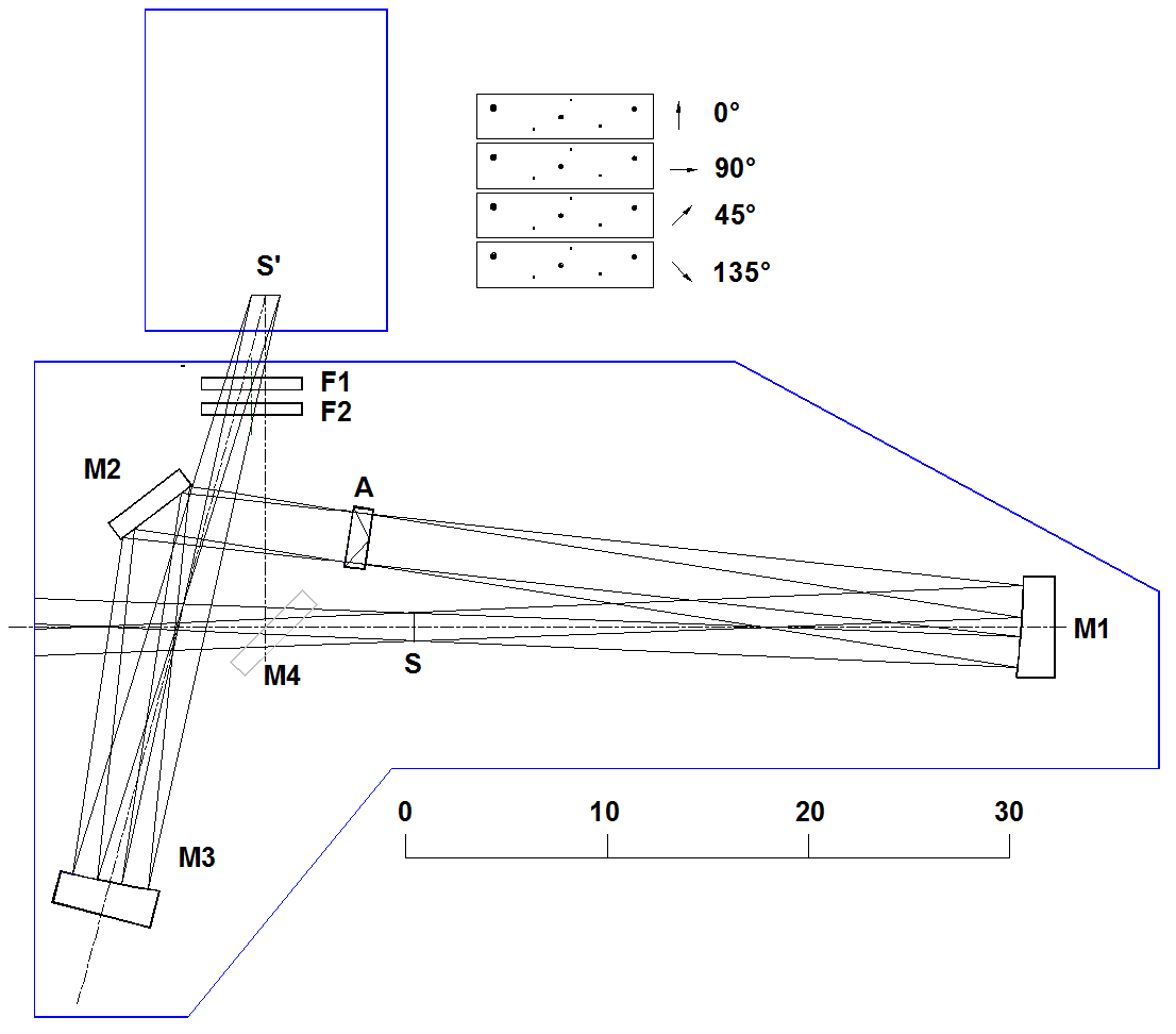
Figure 1: Optical layout of the Stokes-polarimeter: M1, M3 are parabolic off-axis mirrors; M2, M4 are flat diagonal mirrors; A is the polarization analyzer; F1 and F2 are the turrets with replacement filters. The scale at the bottom part of the figure is in centimeter.

The optical layout of the instrument is meant for the use with 13$\times$18 mm Andor Neo sCMOS detector with a pixel size of 6$\times$6 $\mu$m. Note that the long side of the detector must be aligned along the direction of the separation of polarization analyzer beams. However, for a number of reasons—mostly because of photometric properties in long exposures and low quantum efficiency, we stopped using this detector and switched to a low-frame-rate CCD better suited for our task. The detector installed in our instrument is now a 2048$\times$2048 Andor iKon-L 936 CCD with a pixel size of 13.5$\times$13.5 $\mu$m, which corresponds to a scale of 0.21^′′/pix when working with the 1-m telescope. However, appreciable geometric vignetting is observed along the long side of the entrance aperture because of the specificities of the optical layout. The size of non-vignetted field of view in that direction is 19.5 mm. Hence the size of non-vignetted field of view in the polarimetry and photometry modes is 0.9$\times$5^′and 5$\times$7^′, respectively. The CCD used in our instrument has a quantum efficiency greater than 90% in the 400–850 $\mu$m wavelength interval and low readout noise. The operating temperature of the CCD is $-85\hbox{${}^{\circ}$}$C, which ensures that dark noise is lower than readout noise in 5–10 min exposures. The total weight of the instrument together with the turning table is equal to 54 kg.

The transmission of the optical system of the instrument is determined by the reflectivity of mirrors coated with protected silver, which amounts to more than 98% in the optical range, and by Fresnel losses at the surfaces of Wollaston prisms which amount to about 7%. Thus the transmission of the system can be estimated at about 86% when operating in the polarimetry mode (without taking into account the quantum efficiency of the CCD, filter transmission curves, telescope mirror reflectivity).

The control of all mechanical units (switching of filters, inserting/withdrawing diagonal mirrors, turning the instrument along the position angle) is provided by the control board with a microprocessor that is developed to this end. The instrument incorporates a microcomputer, which sends control commands to the instrument and to the CCD controller. During observations the Stokes polarimeter is controlled remotely via Ethernet using a program interface written in IDL.

III MODES OF OBSERVATIONS

III.1 Photometry

As we pointed out in the previous section, the “StoP” instrument can accommodate up to 16 filters, which can be used for photometric observations. We use 250Å-wide medium-band filters to acquire images and estimate fluxes in broad lines (mostly Doppler-shifted H$\alpha$ and H$\beta$) and in the adjacent continuum. Medium-band filters are used to implement the program of AGN reverberation mapping up to redshifts $z\sim 0.8$, and reverberation mapping of Seyfert galaxies in polarized light.

The set of broad-band glass filters allows implementing the Johnson-Cousins $UBVR_{\rm c}I_{\rm c}$ photometric system (Bessell, 1990). To determine the coefficients for transforming instrumental magnitudes into the standard photometric system, we performed on Jaunary 15, 2020 the photometry of stars in the open cluster NGC 2420. Instrumental magnitudes $b,v,r,i$ are computed as $-2.5\log(N)$, where $N$ is the number of counts (ADU) from the object in the corresponding band acquired in the $1.44e^{-}$/ADU gain mode. To transform magnitudes to above-atmosphere values, we determined the extinction coefficients on the same night from observations of the spectrophotometric standard star Feige 34. We found the extinction coefficients to be:

$$\alpha_{B}=0.29^{m}\pm 0.01^{m},$$

$$\alpha_{V}=0.19^{m}\pm 0.01^{m},$$

$$\alpha_{R_{c}}=0.16^{m}\pm 0.01^{m},$$

$$\alpha_{I_{c}}=0.09^{m}\pm 0.01^{m}.$$

We selected 16 cluster stars and compared their measured magnitudes ($bvri$) with published magnitudes ($BVRI$). The transformation equations have the form:

$$B=b+0.08^{\pm 0.03}(B-V)+22.58^{\pm 0.02},$$

$$V=v-0.07^{\pm 0.03}(B-V)+22.85^{\pm 0.02},$$

$$R=r+0.11^{\pm 0.07}(V-R)+22.88^{\pm 0.03},$$

$$I=i-0.04^{\pm 0.06}(V-I)+22.40^{\pm 0.05}.$$

III.2 Polarimetry

Figure 2: Deviation of measured polarization degree values (the left panel) and polarization plane angles (the right panel) from published values for the “StoP” instrument.

Figure 3: Deviation of measured polarization degree values (the left panel) and polarization angles (the right panel) from published values for the MMPP instrument.

The double Wollaston prism in the “StoP” instrument is used as the polarization analyzer. Although the prism was proposed for astronomical observations back in the 1990s (Oliva, 1997; Geyer et al., 1993), it is now rarely used, primarily because the crystal is difficult to make. The advantage of Wollaston prism is that it allows one to simultaneously record four polarization directions—$0^{\circ}$, $90^{\circ}$, $45^{\circ}$, and $135^{\circ}$, and hence the three Stokes parameters $I,Q,U$ that describe the intensity and linear polarization are measured simultaneously. The polarization model of the instrument in the form of the Müller matrix for a similar crystal is presented in formula (3) in Afanasiev and Amirkhanyan (2012). The normalized Stokes parameters $Q$ and $U$ can be computed, up to rotation transformation, by the following formulae:

$$\begin{gathered}\frac{Q}{I}=\frac{I_{0}-I_{90}D_{Q}}{I_{0}+I_{90}D_{Q}},\\ \frac{U}{I}=\frac{I_{45}-I_{135}D_{U}}{I_{45}+I_{135}D_{U}},\end{gathered}$$ (1)

where $D_{Q}$ and $D_{U}$ are the transmission coefficients of the polarization channels. These coefficients take into account both instrumental polarization and atmospheric depolarization (see Afanasiev and Amirkhanyan, 2012, for details). The polarization degree $P$ and the angle of the polarization plane $\varphi$ then are equal to:

$${P}=\sqrt{Q^{2}+U^{2}},$$

$${\varphi^{\prime}}=\frac{1}{2}\arctan Q/U,$$

where ${\varphi^{\prime}}$ is the instrumental angle of polarization plane. To transform it to the true value we use the following formula:

$${\varphi}={\varphi^{\prime}}+{\rm PA}+89.1^{\circ},$$

where ${\rm PA}$ is the position angle of the instrument.

Simultaneous registration of fluxes in four polarization directions allows one to control rapidly varying parameters of atmospheric depolarization and thereby improve the accuracy of polarimetry compared to the use of other analyzers. The only big disadvantage of double Wollaston prism is the need to use a rectangular mask, which decreases the size of the field of view several times. That is why prism is used in spectropolarimetric observations and for the polarimetry of starlike objects like it is done in the case of SCORPIO-2 instrument at the 6-m telescope of the Special Astrophysical Observatory of the Russian Academy of Sciences.

Yet another specific feature of the operation in polarimetry mode is the fact that Wollaston prism has its own dispersion. Chromatic aberrations introduced by the prism distort images in the cross-mask direction and have an angular scale of $\leq$1.5^′′, which is comparable with typical seeing at the Special Astrophysical Observatory. In the case of observations of closely located objects the instrument can be aligned using the turning table so as to prevent the superposition of object images broadened by chromatic aberrations.

The optical system of the instrument uses inclined mirrors, resulting in instrumental polarization. To measure the degree of instrumental polarization over several observational spring sets standard stars with zero polarization were imaged. The zero level of instrumental polarization was found to be 0.74% with across-field variations below 0.1%. The direction of instrumental polarization coincides with that of the mask to within $\pm 3^{\circ}$. Stray light provides no significant contribution to instrumental polarization.

Fig. 2 compares the results of our observations of polarized standards to published data. We found the error of polarization degree and polarization angle to be $({P}_{\rm tab}-{P}_{\rm obs})\sim 0.15\%$ and $({\varphi}_{\rm tab}-{\varphi}_{\rm obs})\sim 0.7^{\circ}$, respectively.

For comparison, we show in Fig. 3 similar dependences of the observed polarization degree and polarization angle on published values for MMPP instrument (Emelianov and Fatkhullin, 2019), which has been used on Zeiss-1000 telescope since 2018 and which was operated in test mode at the time when this paper was written. The polarization analyzer employed is a dichroic polaroid mounted in three positions— $-60^{\circ}$, $0^{\circ}$, and $60^{\circ}$—and producing a field of view with a size of about 6$\times$6^′. Because of non-simultaneous imaging of the object at different polarization directions and slow rotation of the polaroid (up to 20 seconds between the positions) measurements performed using this technique become especially sensitive to weather and their accuracy degrades appreciably. As is evident from the plots, the errors of the inferred polarization degree and polarization angle are equal to $({P}_{\rm tab}-{P}_{\rm obs})\sim 1.1\%$ and $({\varphi}_{\rm tab}-{\varphi}_{\rm obs})\sim 45^{\circ}$, respectively. Such accuracy is insufficient for studying extragalactic objects.

IV OBSERVATIONS

The main task of the “StoP” instrument is to perform high-precision polarimetric observations of starlike objects, and in this sense are unparalleled among attachable equipment for Zeiss-1000 telescope. The technique of the measurement of the polarization of point-like sources with an accuracy of 0.1% was successfully used on the 6-m telescope of the Special Astrophysical Observatory of the Russian Academy of Sciences equipped with SCORPIO-2 instrument (Shablovinskaya and Afanasiev, 2019), where observations involved the use of an analyzer similar to that incorporated in “StoP”—double Wollaston prism WOLL-2. To test the technique of observations we decided to repeat observations of the blazar S5 0716+714.

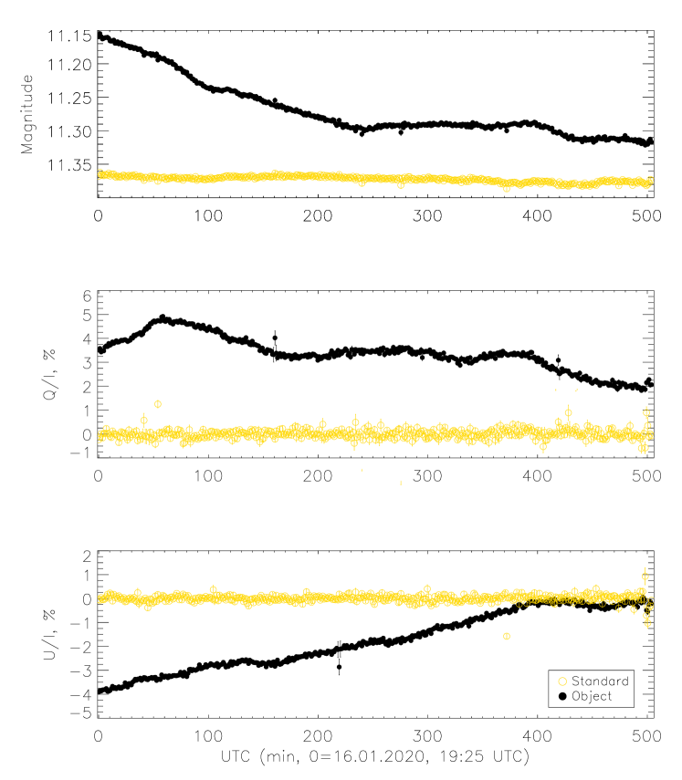
Figure 4: Photometric variations and variations of normalized Stokes parameters $Q$ and $U$ during the night.

On January 16, 2020 the “StoP” instrument attached to Zeiss-1000 telescope was used to perform 8.5-hour monitoring of the blazar S5 0716+714 in polarized light. 4400 frames of 60-second exposure each were acquired separated by readout time no greater than 10 seconds. Observations were made in white light. The mask was aligned so that the field of view would cover two standard stars (Amirkhanyan, 2006) located near the object. The standard stars have constant flux and zero polarization and therefore were used for differential polarimetry of the object. We computed the normalized Stokes parameters by formulae (1) relative to reference stars in the field.

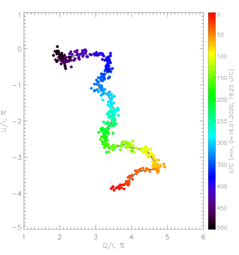
Figure 5: Overnight variations of the normalized Stokes parameters $Q$ and $U$ projected onto the $QU$-plane.

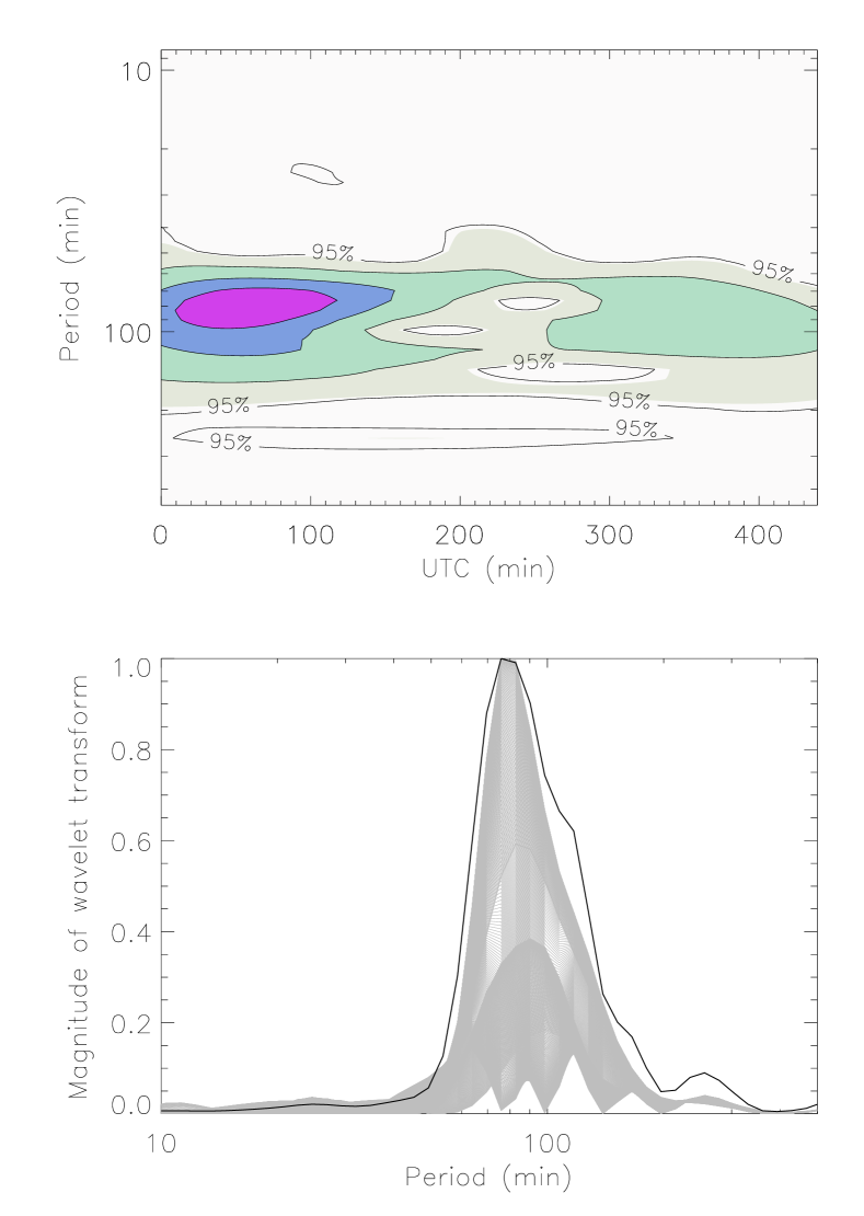
Figure 6: Result of a wavelet analysis of the light curve of the blazar S5 0716+714. The maximum of the profile of the wavelet transform corresponds to the light-variation period of $\sim$76 minutes.

Fig. 4 shows the results of observations. Photometric errors do not exceed $0\hbox{$\,.\!\!^{\rm m}$}005$ and the average error of polarization measurements is 0.05%. Observations in Fig. 5 are shown in the form of the $QU$-diagram where the time elapsed since the start of the observation of the object is coded by color. As is evident from the figure, polarization vector varies smoothly during the night with its direction reversing with a period of about 75 minutes. The same period shows up in the light curve corrected for the long-period trend approximated using local linear-regression algorithm (LOESS). Fig. 6 shows the result of a wavelet analysis of rapid flux variations of the object. Wavelet analysis shows the period of light variations of the object to be 76$\pm$10 minutes. The agreement between the period of light variations and that of the variations of the polarization vector are totally consistent with the result that we earlier obtained based on observations made with the 6-m telescope of the Special Astrophysical Observatory of the Russian Academy of Sciences (Shablovinskaya and Afanasiev, 2019). Thus the observations mentioned above show that the task of the polarimetry of relatively bright (about $13$–$14^{\rm m}$) starlike objects can be successfully addressed with the “StoP” instrument and the accuracy of both photometry and polarimetry are on a par with those of the results obtained with the 6-m telescope.

V CONCLUSIONS

The “StoP” instrument was put into operation in the early 2020. We demonstrate that the instrument can achieve the accuracy needed for the photometric and polarimetric study of extragalactic objects. During the first half-year of its operation significant scientific results were obtained including both those reported in this paper and those submitted to other scientific journals (Malygin et al., 2020). Hence the instrument improves the efficiency of observations and expands the range of observational tasks that can be addressed with the 1-m Zeiss-1000 telescope of the Special Astrophysical Observatory of the Russian Academy of Sciences.

FUNDING

This work was supported by the Russian Science Foundation (grant no.  20-12-00030 “Investigation of geometry and kinematics of ionized gas in active galactic nuclei by polarimetry methods”. Observations were conducted with the telescopes of the Special Astrophysical Observatory of the Russian Academy of Sciences with the financial support of the Ministry of Science and Higher Education of the Russian Federation (including agreement No. 05.619.21.0016, project ID RFMEFI61919X0016).

CONFLICT OF INTEREST

The authors declare no conflict of interest.

Translated by A. Dambis

References

- Afanasiev and Amirkhanyan (2012) V. L. Afanasiev and V. R. Amirkhanyan, Astrophysical Bulletin 67 (4), 438 (2012).
- Afanasiev and Popović (2015) V. L. Afanasiev and L. Č. Popović, Astrophys. J. Letters 800 (2), L35 (2015).
- Amirkhanyan (2006) V. R. Amirkhanyan, Astronomy Reports 50 (4), 273 (2006).
- Ay et al. (2002) S. U. Ay, M. P. Lesser, and E. R. Fossum, SPIE Conf. Ser. 4836, 271 (2002).
- Bessell (1990) M. S. Bessell, Publ. Astron. Soc. Pacific 102, 1181 (1990).
- Cherepashchuk and Lyutyi (1973) A. M. Cherepashchuk and V. M. Lyutyi, Astronomy Letters 13, 165 (1973).
- Emelianov and Fatkhullin (2019) E. V. Emelianov and T. A. Fatkhullin, IX All-Russian Science Conference ¡¡System Analysis and applied synergy¿¿ (Nizhnii Arkhyz, Russia, September 24–27, 2019), 223–228.
- Geyer et al. (1993) E. H. Geyer, N. N. Kiselev, G. P. Chernova, and K. Jockers, IAU Symp. Abstracts 160, 116 (1993).
- Komarov et al. (2020) V. V. Komarov, A. S. Moskvitin, V. D. Bychkov, et al., Astrophysical Bulletin 75 (4), 547 (2020).
- Malygin et al. (2020) E. A. Malygin, E. S. Shablovinskaya, R. I. Uklein, and A. A. Grokhovskaya, Astronomy Letters (in press) (2020).
- Moiseev et al. (2020) A. Moiseev, A. Perepelitsyn, and D. Oparin, Experimental Astronomy 50 (2-3), 199 (2020).
- Oliva (1997) E. Oliva, Astron. and Astrophys. Suppl. 123, 589 (1997).
- Pozo Nuñez et al. (2017) F. Pozo Nuñez, D. Chelouche, S. Kaspi, and S. Niv, Publ. Astron. Soc. Pacific 129 (9), 094101 (2017).
- Shablovinskaya and Afanasiev (2019) E. S. Shablovinskaya and V. L. Afanasiev, Monthly Notices Royal Astron. Soc. 482 (4), 4322 (2019).
- Shablovinskaya et al. (2020) E. S. Shablovinskaya, V. L. Afanasiev, and L. Č. Popović, Astrophys. J. 892 (2), 118 (2020).
- Uklein et al. (2019) R. I. Uklein, E. A. Malygin, E. S. Shablovinskaya, et al., Astrophysical Bulletin 74 (4), 388 (2019).