Minimum variance constrained estimator

Abstract

This paper is concerned with the problem of state estimation for discrete-time linear systems in the presence of additional (equality or inequality) constraints on the state (or estimate). By use of the minimum variance duality, the estimation problem is converted into an optimal control problem. Two algorithmic solutions are described: the full information estimator (FIE) and the moving horizon estimator (MHE). The main result is to show that the proposed estimator is stable in the sense of an observer. The proposed algorithm is distinct from the standard algorithm for constrained state estimation based upon the use of the minimum energy duality. The two are compared numerically on the benchmark batch reactor process model.

1 Introduction

In many practical estimation problems arising in control applications, there are invariably additional constraints on the state process [1]. In such applications, Kalman filter (KF) may yield sub-optimal estimates that violate the constraints. It is notable also that the KF is derived under the assumption of (unbounded) Gaussian noise, which is also unrealistic in the constrained settings of the problem. In particular, in the presence of unbounded noise, local stability results are not applicable and global stability results are very conservative due to actuator saturation [2, 3]. Although clever modifications in KF are still possible [4], the stability and optimality properties of such modifications require further investigation [5]. For these reasons, constrained estimation is a problem of paramount practical importance; c.f., [1] for a book length treatment.

A popular strategy for constrained estimation is based on the use of duality between estimation and optimal control. A practical advantage of converting a constrained estimation problem into a constrained optimal control problem is that model predictive control (MPC) methods, algorithms, and softwares can readily be applied to obtain a solution. The resulting estimation algorithms are referred to as the full information estimator (FIE), when all the observations are used, and is moving horizon estimator (MHE), when a moving window of most recent past observations are used. Practically, a MHE algorithm is preferred because the number of decision variables in the optimization problem do not increase as more observations are collected.

In linear settings of the problem, there are in general two types of duality: the minimum energy (or maximum likelihood) duality and the minimum variance duality. Refer to [6, 7, 8] for more discussion on duality. For the construction of estimators, the minimum energy duality is by far the more popular technique with contributions in [9, 10, 11, 12, 13, 14, 15] and numerical algorithms in [16, 17]. Although minimum variance control has attracted much attention [18, 19, 20], and these recent papers provide motivation also for our work, the use of minimum variance duality for constrained estimation has received comparatively less attention.

State estimation problem for linear systems with equality constraints is considered in [21, 22], and with inequality constraints in [23]. Since the number of decision variables in the underlying optimization program increases as more measurements are collected, an MHE algorithm is proposed in the early work of [24] in the absence of constraints. This algorithm is extended in [25] to incorporate constraints. The stability properties of this constrained MHE algorithm are studied rigorously in [26]. Enhancements of these basic algorithms have been considered both in deterministic (observer design) [27, 28, 29, 30] and stochastic (filter design) [24, 25, 26, 31] settings of the problem. In stochastic settings, the MHE optimal control problem is still deterministic but statistical information about uncertainties and prior are used to design the (maximum likelihood-type) objective function. More recent extensions include a game theoretic formulation in [32]. It is noted that [24, 25, 26, 31, 32] are based on the use of the minimum energy duality. We refer readers to [33, Appendix B] for a quick review of duality and to [34] for minimum energy duality in particular.

In this paper, an alternate form of duality, viz., the minimum variance duality is employed to transform the minimum variance estimation problem into a deterministic optimal control problem. The state estimate is constructed as a linear function of past measurements. Without constraints, the optimal estimate is equivalent to a Kalman filter. Both the FIE and the MHE are described for the unconstrained case, together with expression for choosing the terminal cost in the MHE.

The main focus of this paper is on the modification of these (unconstrained) FIE and MHE algorithms in the presence of constraints. In particular, a certain approximate expression for the terminal cost is introduced for the constrained MHE. The main result of this paper is to establish sufficient conditions to obtain stability (in the sense of an observer) for the constrained FIE and MHE algorithms. Furthermore, we also establish a certain type of stochastic stability by showing that the variance of the constrained FIE converges under certain technical conditions.

Although estimators based on minumum variance duality are less well studied [35], some closely related estimators have appeared in  [36, 37, 31, 38, 39, 40]. In contrast to our paper, these prior works do not incorporate equality or inequality constraint on state (or estimate) in the estimator design. The original contributions of our paper are as follows:

• Based on minimum variance duality, a MHE is presented in (12) and its equivalence with FIE is shown in Lemma 2. This contribution is different from [31, 38] in the sense that unbiasedness constraints are not required. The proposed estimator (13) is equivalent to KF.

• Constrained FIE and MHE algorithms are presented in (16) and (19), respectively. Apart from the fact that these algorithms are distinct from [26], our minimum variance-based approach has certain technical advantages.

• Although the notion of stability is borrowed from [26], Theorems 1 and 2 are first such results on stability of constrained minimum variance estimators.

• Under certain technical conditions, the variance of constrained FIE is shown to converge in Theorem 3.

The remainder of this paper is organized as follows: The problem statement appears in §2 followed by a description of the minimum variance duality for the construction of the unconstrained estimators, both FIE and MHE, in §3.1. These are extended to the constrained case in §3.2. The main results on stability of the constrained FIE and MHE appear in §4. The algorithms are illustrated with the aid of some numerical experiments in §5. The paper closes with some conclusions and directions for future research in §6. All the proofs appear as part of the two appendices,§A and §B, for the unconstrained and the constrained cases, respectively.

Let $\mathds{R},\mathds{N}_{0},\mathds{Z}_{+}$ denote the set of real numbers, the non-negative integers and the positive integers, respectively. We use the symbols $\mathbf{0}$ and $I$ to denote zero matrix and identity matrix, respectively, of appropriate dimensions. For any vector or matrix sequence $(M_{n})_{n\in\mathds{N}_{0}}\in\mathds{R}^{r\times m},r,m\in\mathds{Z}_{+}$, let $M_{n:k}\in\mathds{R}^{rk\times m}$ denote the matrix $\begin{bmatrix}M_{n}^{\top}&M_{n+1}^{\top}&\cdots&M_{n+k-1}^{\top}\end{bmatrix}^{\top}$, $k\in\mathds{Z}_{+}$. Let $\lambda_{\max}(M)$ denote the largest eigenvalue value of $M$, $\lambda_{\min}(M)$ its smallest eigenvalue, $M^{\dagger}$ its Moore-Penrose pseudo inverse and $\operatorname{tr}(M)$ its trace. The Euclidean norm of a vector $A$ is denoted by $\left|A\right|$. The Frobenius norm of a matrix $A$ is denoted by $\left|A\right|_{F}$. A $t$ step reachability matrix of a matrix pair $(A,B)$ is given by $\mathrm{R}_{t}(A,B)\coloneqq\begin{bmatrix}A^{t-1}B&\ldots&AB&B\end{bmatrix}$.

2 Problem statement

Consider a linear discrete-time system

$$x_{t+1} =Ax_{t}+w_{t},$$ (1)

$$y_{t} =Cx_{t}+\varsigma_{t},$$

where $x_{t}\in\bar{\mathcal{X}}\subset\mathds{R}^{d}$, $y_{t}\in\mathds{R}^{q}$ are state and measurement of the system at time $t$, respectively. The system matrix $A\neq\mathbf{0}$. The additive process noise $w_{t}$ and the measurement noise $\varsigma_{t}$ are mean zero, mutually independent and identically distributed random vectors with variance $Q$ and $R$, respectively. The initial state of the system $x_{0}$ is a random vector with mean $\hat{x}_{0}^{-}$ and variance $\Sigma_{0}^{-}$, and is independent of the process noise and the measurement noise.

The minimum variance estimation problem is to compute $\hat{x}_{t}$ at time $t$ such that the variance of error $x_{t}-\hat{x}_{t}$ is minimized over some class of admissible estimators. In this paper, the admissible estimators are assumed to be linear deterministic functions of available measurements. It is also assumed that some additional insight into the states (or estimates) is given in terms of equality and inequality constraints such that the estimated states belong to a convex set $\mathcal{X}\supseteq\bar{\mathcal{X}}$ , i. e. , $\hat{x}_{t}\in\mathcal{X}$ for all $t$. We make the following assumption:

Assumption 1.

The set $\mathcal{X}$ is positively invariant under the nominal dynamics, i. e. , $Ax\in\mathcal{X}\text{ for every }x\in\mathcal{X}$.

The above asssumption is meaningful. Suppose $A\hat{x}_{t}\notin\mathcal{X}$ for some $\hat{x}_{t}\in\mathcal{X}$ then there is a non-zero probability that $x_{t+1}\notin\bar{\mathcal{X}}$ for random $w_{t}$, e.g., when $\hat{x}_{t}=x_{t}$ and a bounded disturbance set with known bounds is not safely prescribed. The optimization problem is as follows:

$$\min_{\hat{x}_{t}\in\mathcal{X}}\quad\mathds{E}\left[\left|x_{t}-\hat{x}_{t}\right|^{2}\right].$$ (2)

The solution approach is based on duality between estimation and control. In the following section, we begin by presenting an unconstrained estimator which is useful for the development of a constrained estimator in §3.2.

3 Minimum variance estimators

3.1 Unconstrained estimator

In this section, we assume $\mathcal{X}=\mathds{R}^{d}$, i.e., the constraints are not present. We are interested in an estimator linearly parameterized in the innovation terms as follows:

$$\hat{x}_{t}=A^{t}\hat{x}_{0}^{-}-\sum_{i=0}^{t}\alpha_{i}^{\top}(y_{t-i}-CA^{t-i}\hat{x}_{0}^{-}),$$ (3)

in which weights $\alpha_{i}\in\mathds{R}^{q\times d}$ are the decision variables for the optimization problem (2). In order to convert the minimum variance estimation objective into an optimal control problem, a dual process (in forward time) is introduced:

$$z_{i+1} =A^{\top}z_{i}+C^{\top}\alpha_{i+1};\quad i=0,\ldots,t-1,$$ (4)

$$z_{0} =I+C^{\top}\alpha_{0},$$

where $z_{i}\in\mathds{R}^{d\times d}$ is a matrix valued dual state and $\alpha_{i}\in\mathds{R}^{q\times d}$ is control signal for the dual process. From (4) we have

$$z_{t}^{\top}=A^{t}+\sum_{i=0}^{t}\alpha_{i}^{\top}CA^{t-i}.$$ (5)

By substituting (5) into (3), we get the following expression:

$$\hat{x}_{t}=z_{t}^{\top}\hat{x}_{0}^{-}-\sum_{i=0}^{t}\alpha_{i}^{\top}y_{t-i}.$$ (6)

A slight modification of the standard result on minimum variance duality [41, Page 238] , in which only the past measurements are used to design an estimator, i. e. $\alpha_{t}=\mathbf{0}$, is required to include the current measurement. Let $\ell_{i}\coloneqq z_{i}^{\top}Qz_{i}+\alpha_{i}^{\top}R\alpha_{i}$, $\Gamma_{0}(z_{t})\coloneqq z_{t}^{\top}\Sigma_{0}^{-}z_{t}$ and

$$S_{t}(\alpha_{0:t+1})\coloneqq\alpha_{t}^{\top}R\alpha_{t}+\sum_{i=0}^{t-1}\ell_{i}.$$ (7)

The estimate (3) takes into account all measurements available at time $t$. Therefore, the corresponding estimator is called full information estimator (FIE). Using the dual process (4), the FIE optimal control problem is expressed as follows:

$$\text{FIE:}\quad\left\{\begin{aligned} \operatorname*{minimize}_{\alpha_{0:t+1}}&\quad\operatorname{tr}(\Gamma_{0}(z_{t})+S_{t}(\alpha_{0:t+1}))\\ \operatorname*{subject\ to}&\quad\text{dual dynamics }\eqref{e:dual_process}.\end{aligned}\right.$$ (8)

FIE (8) is solved at each time $t=0,1,\ldots$. The resulting optimal solution is denoted as $\alpha_{0:t+1\mid t}$, where $\alpha_{k\mid t}$ is the optimal weight $\alpha_{k}$ computed at time $t$. Set

$$\Sigma_{t}\coloneqq\Gamma_{0}(z_{t\mid t})+S_{t}(\alpha_{0:t+1\mid t}),$$ (9)

where $S_{t}(\alpha_{0:t+1\mid t})$ is the optimal value of $S_{t}(\alpha_{0:t+1})$ obtained by solving FIE (8). Then the optimal value of the objective function in (8) is $\operatorname{tr}(\Sigma_{t})$. The estimate $\hat{x}_{t\mid t}$ at time $t$ is obtained by substituting the optimal values $\alpha_{0:t+1\mid t}$ and $z_{t\mid t}$ in (6). In the remainder of the manuscript, we will use $\hat{x}_{t}$ to denote the estimate obtained by substituting the optimizers in (6). We have the following Lemma to show the equivalence of FIE (8) and (2) whenever $\mathcal{X}=\mathds{R}^{d}$.

Lemma 1.

Consider the system (1) and the dual process (4). If $\hat{x}_{t}$ is given by (6) then

$$\mathds{E}\left[\left|x_{t}-\hat{x}_{t}\right|^{2}\right]=\operatorname{tr}(\Gamma_{0}(z_{t})+S_{t}(\alpha_{0:t+1})).$$

Remark 1.

The dual process is typically considered backward in time. However, because the optimal control problem is deterministic, a forward time dual process may equivalently be considered simply by renaming the indices. This is done here to yield the standard form of an optimal control problem where the time arrow is forward.

We present a finite horizon approximation of FIE (8), which we refer to as moving horizon estimator (MHE). For this purpose, define

$$\Sigma_{t}^{-}\coloneqq A\Sigma_{t-1}A^{\top}+Q\text{ and }\hat{x}_{t}^{-}\coloneqq A\hat{x}_{t-1}.$$ (10)

Fix $N\in\mathds{N}_{0}$ and for $t\geqslant N+1$ define

$$\Gamma_{t-N}(z_{N})\coloneqq z_{N}^{\top}\Sigma_{t-N}^{-}z_{N}.$$ (11)

The unconstrained MHE is as follows:

$$\text{MHE:}\quad\left\{\begin{aligned} \operatorname*{minimize}_{\alpha_{0:N+1}}&\quad\operatorname{tr}(\Gamma_{t-N}(z_{N})+S_{N}(\alpha_{0:N+1}))\\ \operatorname*{subject\ to}&\quad\text{dual dynamics }\eqref{e:dual_process}.\end{aligned}\right.$$ (12)

For $t\leqslant N$, set $\Gamma_{t-N}=\Gamma_{0},S_{N}=S_{t}$, which is identical to solving the FIE problem (8). For $t\geqslant N+1$, the MHE problem utilizes the most recent $N+1$ measurements together with the previously computed $\Sigma_{t-N-1}$ to obtain $\Sigma_{t-N}^{-}$. The resulting estimator and the error covariance matrix are

$$\hat{x}_{t} =z_{N\mid t}^{\top}\hat{x}_{t-N}^{-}-\sum_{i=0}^{N}\alpha_{i\mid t}^{\top}y_{t-i},$$ (13)

$$\Sigma_{t} =\operatorname{tr}(\Gamma_{t-N}(z_{N\mid t})+S_{N}(\alpha_{0:N+1\mid t})),$$ (14)

where $\alpha_{i\mid t}$ for $i=0,\ldots,N$, and $z_{N\mid t}$ are obtained by solving MHE (12) at time $t$. It is straightforward to show that, when $N=0$, MHE (12) is the KF. A direct implication of dynamic programming is the following result:

Lemma 2.

If $R\succ 0$ then FIE (8) is equivalent to MHE (12) and the estimate (6) is equal to the estimate (13).

Proofs of lemmas 1 and 2 are given in the Appendix A.

3.2 Constrained estimator

If the matrix pair $(A,C)$ is observable then there exists an integer $n\leqslant d\in\mathds{Z}_{+}$ such that $\operatorname{rank}(\mathrm{R}_{n}(A^{\top},C^{\top}))=d$. The smallest such $n$ is referred to as the observability index of $(A,C)$. Our construction of the constrained FIE depends on $n$. In particular, we augment the FIE (8) with the following additional constraints:

$$z_{t-j}^{\top}\hat{x}_{0}^{-}-\sum_{i=0}^{t-j}\alpha_{i}^{\top}y_{t-j-i}\in\mathcal{X},$$ (15)

where $j=0$ for $t\leqslant n$ and $j=0,\ldots,t-n$, for $t\geqslant n+1$. Note that the left hand side of the constraint is same as $\hat{x}_{t-j}$ according to (6). Although we are interested in this constraint only with $j=0$, inclusion of the intermediate constraints, for $j=1,\ldots,t-n$, helps to ensure some properties. Additional details on this appear in the next section. The constrained FIE problem is formally defined as follows:

$$\text{CFIE:}\quad\left\{\begin{aligned} \operatorname*{minimize}_{\alpha_{0:t+1}}&\quad\operatorname{tr}(\Gamma_{0}(z_{t})+S_{t}(\alpha_{0:t+1}))\\ \operatorname*{subject\ to}&\quad\text{dual dynamics }\eqref{e:dual_process},\\ &\quad\text{constraints }\eqref{e:intermediate constraint}.\end{aligned}\right.$$ (16)

The solution of the CFIE (16) is used to construct the constrained full information estimate by using the right hand side of (6). It is denoted $\hat{x}_{t}^{\text{cf}}$ to distinguish it from unconstrained estimate $\hat{x}_{t}$ obtained by solving (8) or (12). In particular,

$$\hat{x}_{t}^{\text{cf}}\coloneqq z_{t\mid t}^{\top}\hat{x}_{0}^{-}-\sum_{i=0}^{t}\alpha_{i\mid t}^{\top}y_{t-i},$$ (17)

$$\Sigma_{t}^{\text{cf}}\coloneqq\Gamma_{0}(z_{t\mid t})+S_{t}(\alpha_{0:t+1\mid t}),$$

where $z_{t\mid t}$ and $\alpha_{0:t+1\mid t}$ are obtained by solving (16).

Remark 2 (Feasibility and convexity).

If $\hat{x}_{0}^{-}\in\mathcal{X}$ then the optimal control problem (16) is feasible for all $t$ because $\alpha_{0:t+1}=\mathbf{0}$ satisfies (15). The left hand side of (15) is affine in decision variables $\alpha_{0:t+1}$ and the set $\mathcal{X}$ is convex. The set of decision variables $\alpha_{0:t+1}$ in (15) is convex due to the fact that the inverse image of a convex set under an affine function is convex [42, Page 38] and the intersection of convex sets is convex.

Remark 3.

The right hand side of (6) is linear in the past measurements. The justification comes from the unconstrained linear Gaussian case where such a structure is sufficient to obtain the minimum variance estimator. In the presence of constraints and non-Gaussian noise, an optimal estimate may not be linear in the past measurements. It is noted that the assumed structure is also nonlinear because of the dependance of $\alpha_{0:t+1}$ on $y_{0:t+1}$ via constraint (15).

In the presence of constraints, the design of an MHE algorithm, that is provably equivalent to the FIE algorithm, is challenging because of the difficulty in approximating the terminal cost. Therefore, approximation of the terminal cost (which is also referred to as arrival cost in the standard MHE literature) is necessary. The goal is to approximate the FIE as closely as possible while maintaining computational tractability and guaranteeing stability.

Similar to CFIE (16), constrained MHE can also be defined by adding extra constraints to the unconstrained MHE (12). The constrained MHE estimator is denoted as $\hat{x}_{t}^{\text{cm}}$, where the superscript cm is used to reflect the fact that this estimate at time $t$ may be different from the unconstrained estimate $\hat{x}_{t}$ and the CFIE estimate $\hat{x}_{t}^{\text{cf}}$. Similarly, the corresponding error covariance matrix is denoted by $\Sigma_{t}^{\text{cm}}$ to distinguish it from (14).

We need to define priors $\Sigma_{t-N}^{\text{cm}-}$ and $\hat{x}_{t-N}^{\text{cm}-}$ to compute the terminal cost of the constrained MHE and its estimate as we did in (11) and (13), respectively, for the unconstrained case. One possible choice is to use $\Sigma_{t-N}^{-}$ and $\hat{x}_{t-N}^{-}$ obtained from the unconstrained case by using (10) and (12), which is same as running a KF in parallel. The standard MHE [26] follows this approach. Other MHE approaches like [29] also use priors from the unconstrained case. Since our approach not only gives an estimated state which satisfies constraints but also an error covariance matrix, it is reasonable to replace $\Sigma_{t-1}$ in (10) by $\Sigma_{t-1}^{\text{cm}}$ to get $\Sigma_{t}^{\text{cm}-}$ and $\hat{x}_{t-1}$ by $\hat{x}_{t-1}^{\text{cm}}$ to get $\hat{x}_{t}^{\text{cm}-}$. This choice is intuitive because the pair $(\hat{x}_{t}^{\text{cm}-},\Sigma_{t}^{\text{cm}-})$ represents our prior knowledge about the pair $(\hat{x}_{t}^{\text{cm}},\Sigma_{t}^{\text{cm}})$ in the presence of constraints. More precisely,

$$\Sigma_{t}^{\text{cm}-}\coloneqq A\Sigma_{t-1}^{\text{cm}}A^{\top}+Q\text{ and }\hat{x}_{t}^{\text{cm}-}\coloneqq A\hat{x}_{t-1}^{\text{cm}}.$$ (18)

The constrained MHE problem is formally written as follows:

$$\text{CMHE:}\quad\left\{\begin{aligned} \operatorname*{minimize}_{\alpha_{0:N+1}}&\quad\operatorname{tr}(\Gamma_{t-N}^{\text{cm}}(z_{N})+S_{N}(\alpha_{0:N+1}))\\ \operatorname*{subject\ to}&\quad\text{dual dynamics }\eqref{e:dual_process},\text{ and }\\ &\quad z_{N}^{\top}\hat{x}_{t-N}^{\text{cm}-}-\sum_{i=0}^{N}\alpha_{i}^{\top}y_{t-i}\in\mathcal{X},\end{aligned}\right.$$ (19)

where $\Gamma_{t-N}^{\text{cm}}(z_{N})\coloneqq z_{N}^{\top}\Sigma_{t-N}^{\text{cm}-}z_{N}$ for $t\geqslant N+1$. Similar to MHE (12) for $t\leqslant N$, we set $\Gamma_{t-N}^{\text{cm}}=\Gamma_{0},S_{N}=S_{t}$ and similarly modify constraint by taking all $t+1$ measurements. Alternatively, we can run CFIE (16) for $t\leqslant N$. Further, the estimate (6) and corresponding covariance matrix can be written as

$$\hat{x}_{t}^{\text{cm}}\coloneqq z_{N\mid t}^{\top}\hat{x}_{t-N}^{\text{cm}-}-\sum_{i=0}^{N}\alpha_{i\mid t}^{\top}y_{t-i},$$ (20)

$$\Sigma_{t}^{\text{cm}}\coloneqq\Gamma_{t-N}^{\text{cm}}(z_{N\mid t})+S_{N}(\alpha_{0:N+1\mid t}),$$

where $\alpha_{i\mid t}$ for $i=0,\ldots,N$, and $z_{N\mid t}$, are obtained by solving CMHE problem (19) at time $t$.

4 Main results

In this section, stability of the proposed constrained estimators is presented by using the notion of stability introduced in [26]. Recall that the classical notion of stability of an observer is obtained by modifying the definition of the stability of a regulator. In an analogous manner, the definition of the stability of a constrained regulator, which is given in [43, §2], is modified in [26] to introduce the following definition:

Definition 1 ([26, 43]).

The estimator is a stable observer for the system

$$x_{t+1} =Ax_{t};\quad y_{t}=Cx_{t};\quad x_{t}\in\mathcal{X},$$ (21)

if for any $\varepsilon>0$, there exists $\delta>0$ and $T\in\mathds{Z}_{+}$ such that if $\hat{x}_{0}^{-}\in\mathcal{X}$ and $\left|x_{0}-\hat{x}_{0}^{-}\right|\leqslant\delta$ then $\left|\hat{x}_{t}-A^{t}x_{0}\right|\leqslant\varepsilon$ for all $t\geqslant T$. If in addition, $\hat{x}_{t}\rightarrow A^{t}x_{0}$ as $t\rightarrow\infty$ then the estimator is called asymptotically stable observer for the system (21).

Our approach has a minor advantage over [26] in the sense that a key assumption is relaxed. In particular, we do not assume any upper bound on cost a priori but it comes naturally from the observability of the system. For the stability of CFIE we need one of the following two conditions to hold:

1. $Q-\Sigma_{0}^{-}\succeq 0$.

2. There exists some $K_{t}\in\mathds{R}^{q\times d}$ at each time $t\geqslant n+1$ such that $\alpha_{t}=K_{t}z_{t-1\mid t-1}$ satisfies (15) for $j=0$ and the following stability criterion with $\tilde{A}_{t}=A^{\top}+C^{\top}K_{t}$:

   $$\tilde{A}_{t}^{\top}\Sigma_{0}^{-}\tilde{A}_{t}-\Sigma_{0}^{-}\preceq-(K_{t}^{\top}RK_{t}+Q).$$ (22)

The main stability result for the CFIE is as follows:

Theorem 1.

Suppose Assumption 1 holds, $\left|\hat{x}_{0}^{-}-x_{0}\right|<\infty$, $\Sigma_{0}^{-}\succ 0$, $(A,C)$ is observable, and one of the two conditions, either (C1) or (C2), is satisfied. Then CFIE is an asymptotically stable observer for the system (21).

Remark 4.

It is easily verified that the conditions (C1) and (C2) can not simultaneously hold unless $A=\mathbf{0}$, which because the matrix pair $(A,C)$ is observable, represents a trivially false case. Let, if possible, (C1) and (C2) hold simultaneously then (C2) gives

$$0\preceq\tilde{A}_{t}^{\top}\Sigma_{0}^{-}\tilde{A}_{t}\preceq-(K_{t}^{\top}RK_{t}+Q-\Sigma_{0}^{-})\preceq 0,$$ (23)

which implies $\tilde{A}_{t}^{\top}\Sigma_{0}^{-}\tilde{A}_{t}=K_{t}^{\top}RK_{t}+Q-\Sigma_{0}^{-}=\mathbf{0}$. Therefore, $\tilde{A}_{t}=\mathbf{0}$ because $\Sigma_{0}^{-}\succ 0$ and $K_{t}^{\top}RK_{t}+Q=\Sigma_{0}^{-}$, which results in $Q\preceq\Sigma_{0}^{-}$ and due to (C1) we get $Q=\Sigma_{0}^{-}$. By substituting $Q=\Sigma_{0}^{-}$ in (23), we get $K_{t}^{\top}RK_{t}=\mathbf{0}$, which results in $K_{t}=\mathbf{0}$ because $R\succ 0$. Since $\tilde{A}_{t}=\mathbf{0}$ due to (23), the substitution of $K_{t}=\mathbf{0}$ shows that $A=\mathbf{0}$.

We have the following result on stability of CMHE:

Theorem 2.

Suppose Assumption 1 holds, $\Sigma_{0}^{-}\succ 0$, $R\succ 0$ and $(A,C)$ is observable then for $N\geqslant n$, CMHE is stable observer for the system (21). If, in addition, $Q\succ 0$, $\left|\hat{x}_{0}^{-}-x_{0}\right|<\infty$, then CMHE is asymptotically stable observer for the system (21).

In theorems 1 and 2, we proved stability of the proposed estimators in the sense of an observer. Since the cost function represents variance in the proposed approach, we get its convergence for the system (1) also under the following assumption:

Assumption 2.

There exist $\alpha_{0}\in\mathds{R}^{q\times d}$, and a sequence of matrices $(K_{i})_{i\in\mathds{Z}_{+}}$ such that $\alpha_{i+1}=K_{i}z_{i}$ and $\alpha_{0}$ satisfy (15). There exist $\lambda_{0}>0$, $\lambda_{i}<1$ for $i\in\mathds{Z}_{+}$ such that

1. $(I+C^{\top}\alpha_{0})^{\top}Q(I+C^{\top}\alpha_{0})+\alpha_{0}^{\top}R\alpha_{0}\leqslant\lambda_{0}Q$

2. $(A^{\top}+C^{\top}K_{i})^{\top}Q(A^{\top}+C^{\top}K_{i})+K_{i}^{\top}RK_{i}\leqslant\lambda_{i}Q\text{ for }i\in\mathds{Z}_{+}$

The above assumption gives a sufficient condition for the feasibility of (16) and the existence of a stabilizing controller for the dual process (4). Notice that (16) is feasible due to the Remark 2. The above assumption helps us to get an upper bound of the cost in (16). We have the following result:

Theorem 3.

If $\hat{x}_{0}^{-}\in\mathcal{X}$, (A,C) is observable and for all $t\geqslant n+1$ either (C1) with Assumption 2 hold or (C2) is satisfied, then there exists $s^{\prime}\geqslant 0$ such that

$$\mathds{E}\left[\left|x_{t}-\hat{x}_{t}^{\text{cf}}\right|^{2}\right]\longrightarrow s^{\prime}.$$ (24)

Proofs of theorems 1, 2 and 3 are given in Appendix B.

5 Numerical experiments

For numerical experiments, we consider the benchmark model of a well-mixed, constant volume, isothermal batch reactor. This model has previously been considered in [44, 29]. The system dynamics is given by (1), where

$$A=\begin{bmatrix}0.8831&0.0078&0.0022\\ 0.1150&0.9563&0.0028\\ 0.1178&0.0102&0.9954\end{bmatrix},\quad C=\begin{bmatrix}32.84&32.84&32.84\end{bmatrix}$$

The observability index of $(A,C)$ is $3$. The additive process and measurement noise are both assumed to be Gaussian with zero means, and variances, $(0.01)^{2}I$ and $(0.25)^{2}$, respectively. The mean of the initial prior is $\hat{x}_{0}^{-}=\begin{bmatrix}1&1&4\end{bmatrix}^{\top}$. Since the states represent concentration of chemicals in the batch reactor process, these cannot be negative. Therefore, the estimated states are constrained to lie in the set $\mathcal{X}\coloneqq\{x\in\mathds{R}^{d}\mid x\geqslant 0\}$.

Experiment 1.

In the first experiment, we assume that initial state is also Gaussian with prior mean $\hat{x}_{0}^{-}$ and prior variance $\Sigma_{0}^{-}=I$. This is evident that simulated state of the system can be negative due to the presence of Gaussian noises in simulation but we consider this example for a fair comparison with minimum energy MHE (MEMHE) [26].

We demonstrate a comparison between MEMHE and our proposed approach CMHE in Fig. 1. MEMHE is simulated by using nmhe object of freely available MATLAB based software package mpctools [45], which is based on CasAdi [46] and solver Ipopt [47]. For CMHE, we use MATLAB-based software package YALMIP [48] and a solver SDPT3-4.0 [49] to solve the underlying optimization programs. We chose the optimization horizon $N=4$ for both approaches and simulated for $N_{s}=1000$ sample paths. The empirical mean squared error $e_{t}$ for both approaches is computed by the following formula:

$$e_{t}=\frac{1}{N_{s}}\sum_{i=1}^{N_{s}}\left|x_{t}^{i}-\hat{x}_{t}^{i}\right|^{2},$$ (25)

where $x_{t}^{i}$ and $\hat{x}_{t}^{i}$ denote the simulated and estimated states, respectively, at time $t$ in the $i^{\text{th}}$ path.

Fig. 1 depicts that empirical mean squared error in our approach is smaller than that in MEMHE. Interestingly, at $t=0$ both approaches have almost same $e_{t}$ but in our approach it immediately drops by approximately one unit and keeps monotonically decreasing after then. However, in case of MEMHE a slight increase is observed at $t=2$ and after that it monotonically decreases but always remains higher than that of our approach.

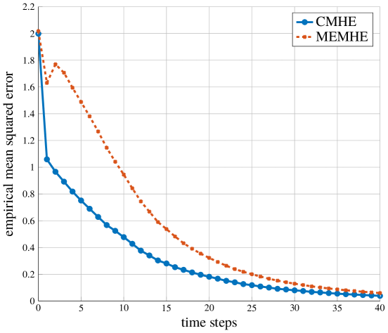
Figure 1: The empirical mean squared error for 1000 sample paths is smaller in our proposed approach than that in standard MHE when initial state has Gaussian distribution.

Experiment 2.

In this experiment, we consider initial state to be uniformly distributed between $[0,2\hat{x}_{0}^{-}]$. Rest of the simulation data is same as in Experiment 1. We simulate for $N_{s}=100$ sample paths and compare between our proposed approach CMHE and standard MEMHE in Fig. 2. The empirical mean squared error $e_{t}$ is computed according to (25). Fig. 2 depicts that both approaches have almost the same empirical mean squared error for 100 sample paths.

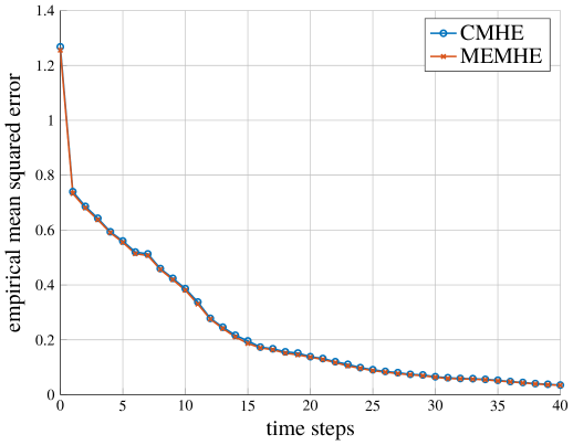
Figure 2: The empirical mean squared error for 100 sample paths is almost same in our proposed approach and standard MHE when initial state has uniform distribution.

Experiment 3.

In this experiment, we choose optimization horizon $N=3$ and simulate only for one sample path. Rest of the simulation data is same as in Experiment 2. We compare the norm of estimate and cost by using CMHE and CFIE in Fig. 3. Both approaches give almost same estimate and incur almost same cost even though the optimization problem of CFIE has intermediate constraints, which are absent in CMHE.

Figure 3: Norm of estimate and optimal cost in both CMHE and CFIE are almost same.

6 Conclusions and directions for future research

In this paper, the minimum variance duality is used to convert the minimum variance estimation problem into a deterministic optimal control problem. The main contribution is the specification and the stability analysis of the FIE and MHE algorithms in the presence of state constraints. The proposed algorithms are distinct from and possess several useful features compared to the standard MHE algorithms based on the use of the minimum energy duality. In particular, there is no need to run a KF in parallel to approximate the terminal cost for the MHE. Both the constrained FIE and MHE algorithms are stable in the sense of an observer. Moreover, stochastic stability of constrained FIE is also established.

This work opens up several avenues for future research: Some ideas of linear model predictive control with time varying terminal cost and constraints  [50], and approximate dynamic programming methods with accumulating constraints [51] may be useful for the further study of the constrained MHE. Several interesting extensions of the proposed approach may be possible including control design [9], systems with intermittent observations [52], distributed architecture [11], the problem of unknown prior [31, 53] and inclusion of pre-estimating observer [27, 31, 54].

Appendix A Proofs of §3.1

Proof of Lemma 1.

Since $z_{0}-C^{\top}\alpha_{0}=I$, we have

$$x_{t}=(z_{0}-C^{\top}\alpha_{0})^{\top}x_{t}=z_{0}^{\top}x_{t}-\alpha_{0}^{\top}Cx_{t}.$$ (26)

By using the system dynamics (1) and the dual dynamics (4), we get

$$z_{i}^{\top}x_{t-i} =z_{i}^{\top}(Ax_{t-i-1}+w_{t-i-1})$$ (27)

$$z_{i+1}^{\top}x_{t-i-1} =z_{i}^{\top}Ax_{t-i-1}+\alpha_{i+1}^{\top}Cx_{t-i-1}.$$

We substitute (27) in the expression of $z_{0}^{\top}x_{t}$ as follows:

$$z_{0}^{\top}x_{t}=\sum_{i=0}^{t-1}(z_{i}^{\top}x_{t-i}-z_{i+1}^{\top}x_{t-i-1})+z_{t}^{\top}x_{0}$$

$$z_{0}^{\top}x_{t}=\sum_{i=0}^{t-1}\left(z_{i}^{\top}w_{t-i-1}-\alpha_{i+1}^{\top}Cx_{t-i-1}\right)+z_{t}^{\top}x_{0}.$$

We further substitute $z_{0}^{\top}x_{t}$ in (26) to get

$$x_{t}=\sum_{i=0}^{t-1}z_{i}^{\top}w_{t-i-1}-\sum_{i=0}^{t}\alpha_{i}^{\top}Cx_{t-i}+z_{t}^{\top}x_{0}$$

$$x_{t}=\sum_{i=0}^{t-1}z_{i}^{\top}w_{t-i-1}-\sum_{i=0}^{t}\alpha_{i}^{\top}(y_{t-i}-\varsigma_{t-i})+z_{t}^{\top}x_{0}.$$

Further, we consider the estimate (6) and compute $\mathds{E}[(x_{t}-\hat{x}_{t})(x_{t}-\hat{x}_{t})^{\top}]$ as follows:

$$x_{t}-\hat{x}_{t}=z_{t}^{\top}\left(x_{0}-\hat{x}_{0}^{-}\right)+\sum_{i=0}^{t-1}z_{i}^{\top}w_{t-i-1}+\sum_{i=0}^{t}\alpha_{i}^{\top}\varsigma_{t-i}$$

$$\mathds{E}[(x_{t}-\hat{x}_{t})(x_{t}-\hat{x}_{t})^{\top}]=z_{t}^{\top}\Sigma_{0}^{-}z_{t}+\sum_{i=0}^{t-1}z_{i}^{\top}Qz_{i}+\sum_{i=0}^{t}\alpha_{i}^{\top}R\alpha_{i}$$

$$\quad\quad=z_{t}^{\top}\Sigma_{0}^{-}z_{t}+\alpha_{t}^{\top}R\alpha_{t}+\sum_{i=0}^{t-1}\ell_{i}=\Gamma_{0}(z_{t})+S_{t}(\alpha_{0:t+1}),$$

since the process noise, measurement noise and initial states are mutually independent. Therefore, $\mathds{E}\left[\left|x_{t}-\hat{x}_{t}\right|^{2}\right]=\operatorname{tr}\left(\Gamma_{0}(z_{t})+S_{t}(\alpha_{0:t+1})\right)$, where $z_{t}$ is obtained by (4) and $\hat{x}_{t}$ is given by (6). ∎

Proof of Lemma 2.

At $t=0$, we compute

$$\Gamma_{0}(z_{0}) +S_{0}(\alpha_{0})=z_{0}^{\top}\Sigma_{0}^{-}z_{0}+\alpha_{0}^{\top}R\alpha_{0}$$

$$=\Sigma_{0}^{-}+\alpha_{0}^{\top}(R+C\Sigma_{0}^{-}C^{\top})\alpha_{0}+\Sigma_{0}^{-}C^{\top}\alpha_{0}+\alpha_{0}^{\top}C\Sigma_{0}^{-}.$$

Since $\alpha_{0\mid 0}=\operatorname*{arg\ min}\operatorname{tr}(\Gamma_{0}(z_{0})+S_{0}(\alpha_{0}))=-(C\Sigma_{0}^{-}C^{\top}+R)^{-1}C\Sigma_{0}^{-}$, due to our convention (9) we obtain $\Sigma_{0}=$

$$\Gamma_{0}(z_{0\mid 0})+S_{0}(\alpha_{0\mid 0})=\Sigma_{0}^{-}-\Sigma_{0}^{-}C^{\top}(C\Sigma_{0}^{-}C^{\top}+R)^{-1}C\Sigma_{0}^{-}.$$ (28)

The FIE cost can be written as

$$\operatorname{tr}(\Gamma_{0}(z_{t})+S_{t}(\alpha_{0:t+1}))=\operatorname{tr}\left(\Gamma_{0}(z_{t})+\alpha_{t}^{\top}R\alpha_{t}+\sum_{i=0}^{t-1}\ell_{i}\right)$$

$$=\operatorname{tr}\left(z_{t}^{\top}\Sigma_{0}^{-}z_{t}+\alpha_{t}^{\top}R\alpha_{t}+z_{t-1}^{\top}Qz_{t-1}+S_{t-1}(\alpha_{0:t})\right).$$

We substitute $z_{t}=A^{\top}z_{t-1}+C^{\top}\alpha_{t}$ in the above expression and the minimizer $\alpha_{t\mid t}^{\top}=-z_{t-1\mid t}^{\top}A\Sigma_{0}^{-}C^{\top}(C\Sigma_{0}^{-}C^{\top}+R)^{-1}$. Further, by substituting $\Sigma_{0}$ from (28), we get

$$\operatorname{tr}(\Gamma_{0}(z_{t})+S_{t}(\alpha_{0:t+1}))=\operatorname{tr}\left(z_{t-1}^{\top}(A\Sigma_{0}A^{\top}+Q)z_{t-1}+S_{t-1}(\alpha_{0:t})\right)$$

$$=\operatorname{tr}\left(z_{t-1}^{\top}\Sigma_{1}^{-}z_{t-1}+S_{t-1}(\alpha_{0:t})\right),$$ (29)

where the last equality is due to our definition (10). Therefore, $\Gamma_{1}(\cdot)$ can be written as $\Gamma_{1}(z_{t-1})=z_{t-1}^{\top}\Sigma_{1}^{-}z_{t-1}$. The above expression of cost (A) at time $t=1$ gives $\Sigma_{1}=z_{0\mid 1}^{\top}\Sigma_{1}^{-}z_{0\mid 1}+S_{0}(\alpha_{0\mid 1})$, where $\alpha_{0\mid 1}=-(C\Sigma_{1}^{-}C^{\top}+R)^{-1}C\Sigma_{1}^{-}$. By repeating the above process $t-N$ times, we obtain

$$\operatorname{tr}(\Gamma_{0}(z_{t})+S_{t}(\alpha_{0:t+1})=\operatorname{tr}\left(z_{N}^{\top}\Sigma_{t-N}^{-}z_{N}+S_{N}(\alpha_{0:N+1})\right),$$

and therefore, we can define $\Gamma_{t-N}(z_{N})=z_{N}^{\top}\Sigma_{t-N}^{-}z_{N}$. Now for $t\geqslant N>0$, we consider the expression of $\hat{x}_{t}$:

$$\hat{x}_{t}=z_{t\mid t}^{\top}\hat{x}_{0}^{-}-\alpha_{t\mid t}^{\top}y_{0}-\sum_{i=0}^{t-1}\alpha_{i\mid t}^{\top}y_{t-i},\text{ where}$$

$$z_{t\mid t}^{\top}\hat{x}_{0}^{-}-\alpha_{t\mid t}^{\top}y_{0}=z_{t-1\mid t}^{\top}A\hat{x}_{0}^{-}-\alpha_{t\mid t}^{\top}(y_{0}-C\hat{x}_{0}^{-}).$$

By substituting $\alpha_{t\mid t}$ in the above expression, we get $z_{t\mid t}^{\top}\hat{x}_{0}^{-}-\alpha_{t\mid t}^{\top}y_{0}=z_{t-1\mid t}^{\top}\left(A\hat{x}_{0}^{-}+A\Sigma_{0}^{-}C^{\top}(C\Sigma_{0}^{-}C^{\top}+R)^{-1}(y_{0}-C\hat{x}_{0}^{-})\right)=z_{t-1\mid t}^{\top}A\hat{x}_{0}$, which implies $\hat{x}_{t}=z_{t-1\mid t}^{\top}\hat{x}_{1}^{-}-\sum_{i=0}^{t-1}\alpha_{i\mid t}^{\top}y_{t-i}$, where $\hat{x}_{1}^{-}=A\hat{x}_{0}$. At $t=1$, we can compute $\hat{x}_{1}^{-}$ from the above expression. By repeating the above process $t-N$ times we obtain the desired expression (13). ∎

Appendix B Proofs of §3.2

Lemma 3.

If (C1) holds then $\operatorname{tr}(\Sigma_{t}^{\text{cf}})\geqslant\operatorname{tr}(\Sigma_{t-1}^{\text{cf}})$ for all $t\geqslant n+1$.

Proof.

Let us define $s_{t}^{\ast}\coloneqq\operatorname{tr}(\Sigma_{t}^{\text{cf}})$ for notational simplicity. The optimal cost at time $t$ by substituting $S_{t}(\alpha_{0:t+1\mid t})=\alpha_{t\mid t}^{\top}R\alpha_{t\mid t}+\sum_{i=0}^{t-1}\ell_{i\mid t}$ in (17) is given by

$$s_{t}^{\ast}=\operatorname{tr}\left(\Gamma_{0}(z_{t\mid t})+\alpha_{t\mid t}^{\top}R\alpha_{t\mid t}+\sum_{i=0}^{t-1}\ell_{i\mid t}\right),$$ (30)

where $\ell_{i\mid t}\coloneqq z_{i\mid t}^{\top}Qz_{i\mid t}+\alpha_{i\mid t}^{\top}R\alpha_{i\mid t}$. We can observe for all $t\geqslant n+1$ that the constraints (15) at time $t-1$ are same at time $t$ for $j=0,\ldots,t-n-1$. Therefore, $\alpha_{0:t\mid t}$, the first $t$ number of decision variables computed at time $t$, is a feasible control sequence at time $t-1$. Due to the optimality of $\alpha_{0:t\mid t-1}$ at time $t-1$, we get the following inequality:

$$s_{t-1}^{\ast} \leqslant\operatorname{tr}\left(\Gamma_{0}(z_{t-1\mid t})+\alpha_{t-1\mid t}^{\top}R\alpha_{t-1\mid t}+\sum_{i=0}^{t-2}\ell_{i\mid t}\right)$$

$$=\operatorname{tr}\left(z_{t-1\mid t}^{\top}(\Sigma_{0}^{-}-Q)z_{t-1\mid t}+\sum_{i=0}^{t-1}\ell_{i\mid t}\right)$$

$$=\operatorname{tr}\left(z_{t-1\mid t}^{\top}(\Sigma_{0}^{-}-Q)z_{t-1\mid t}-\Gamma_{0}(z_{t\mid t})-\alpha_{t\mid t}^{\top}R\alpha_{t\mid t}\right)+s_{t}^{\ast},$$

where the last equality is obtained by substituting (30). Since $Q-\Sigma_{0}^{-}\succeq 0$, for all $t\geqslant n+1$ we get

$$s_{t}^{\ast}-s_{t-1}^{\ast}\geqslant\operatorname{tr}\left(\Gamma_{0}(z_{t\mid t})+\alpha_{t\mid t}^{\top}R\alpha_{t\mid t}+z_{t-1\mid t}^{\top}(Q-\Sigma_{0}^{-})z_{t-1\mid t}\right)\geqslant 0.$$

∎

Lemma 4.

If (C2) holds, then $\operatorname{tr}(\Sigma_{t}^{\text{cf}})\leqslant\operatorname{tr}(\Sigma_{t-1}^{\text{cf}})$ for all $t\geqslant n+1$.

Proof.

We can observe that $\alpha_{0:t\mid t-1}$ satisfies (15) at time $t$ for $j=1,\ldots,t-n$. We assumed that $\alpha_{t}=K_{t}z_{t-1\mid t-1}$ satisfies (15) for $j=0$. Therefore, the control sequence $\alpha_{0:t\mid t-1}$ along with $\alpha_{t}=K_{t}z_{t-1\mid t-1}$ is a feasible control sequence at time $t$. We compute $z_{t}$ by substituting $\alpha_{0:t\mid t-1}$ and $\alpha_{t}$ in (4), which gives us $z_{t}=A^{\top}z_{t-1\mid t-1}+C^{\top}K_{t}z_{t-1\mid t-1}=\tilde{A}z_{t-1\mid t-1}$. Now we recall the expression of the optimal cost $s_{t}^{\ast}\coloneqq\operatorname{tr}(\Sigma_{t}^{\text{cf}})$ from (30). The optimaliity of $\alpha_{0:t+1\mid t}$ in the presence of stability criterion (22) gives us

$$s_{t}^{\ast}\leqslant\operatorname{tr}\left(\Gamma_{0}(\tilde{A}_{t}z_{t-1\mid t-1})+z_{t-1\mid t-1}^{\top}K_{t}^{\top}RK_{t}z_{t-1\mid t-1}+\sum_{i=0}^{t-1}\ell_{i\mid t-1}\right)$$

$$=\operatorname{tr}\left(z_{t-1\mid t-1}^{\top}(\tilde{A}_{t}^{\top}\Sigma_{0}^{-}\tilde{A}_{t}+K_{t}^{\top}RK_{t}+Q)z_{t-1\mid t-1}\right)$$

$$\quad+\operatorname{tr}\left(\alpha_{t-1\mid t-1}^{\top}R\alpha_{t-1\mid t-1}+\sum_{i=0}^{t-2}\ell_{i\mid t-1}\right)$$

$$\leqslant\operatorname{tr}\left(\Gamma_{0}(z_{t-1\mid t-1})+\alpha_{t-1\mid t-1}^{\top}R\alpha_{t-1\mid t-1}+\sum_{i=0}^{t-2}\ell_{i\mid t-1}\right)=s_{t-1}^{\ast}.$$

∎

Lemma 5.

If the Assumption 1 holds and the matrix pair $(A,C)$ is observable then there exists $s>0$ such that for the system (21),

$$\operatorname{tr}(\Sigma_{t}^{\text{cf}}) \leqslant s\text{ for all }t\text{ and}$$

$$\operatorname{tr}(\Sigma_{t}^{\text{cm}}) \leqslant s\text{ for all }N\geqslant n\text{ for all }t.$$

Proof.

Let us consider the expression of $z_{t}$ at $t=n$ from (5). We can write it in compact form: $z_{n}=A^{\top n}(I+C^{\top}\alpha_{0})+\mathrm{R}_{n}(A^{\top},C^{\top})\alpha_{1:n}$. If we substitute

$$\alpha_{1:n}=-\mathrm{R}_{n}(A^{\top},C^{\top})^{\dagger}(A^{\top n})(I+C^{\top}\alpha_{0})$$ (31)

in the above expression for some $\alpha_{0}\in\mathds{R}^{q\times d}$, we get $z_{n}=\mathbf{0}$. Now we consider the estimator (3) and the nominal system (21). By substituting $y_{i}=CA^{i}x_{0}$ and $x_{t}=A^{t}x_{0}$ for the system (21) in (3), we get

$$\hat{x}_{t} =A^{t}(\hat{x}_{0}^{-}-x_{0})+A^{t}x_{0}+\sum_{i=0}^{t}\alpha_{i}^{\top}CA^{t-i}(\hat{x}_{0}^{-}-x_{0})$$

$$=x_{t}+\left(A^{t}+\sum_{i=0}^{t}\alpha_{i}^{\top}CA^{t-i}\right)(\hat{x}_{0}^{-}-x_{0})$$

$$=x_{t}+z_{t}^{\top}(\hat{x}_{0}^{-}-x_{0}),$$ (32)

where the last equality is due to (5). If we substitute $\alpha_{1:n}$ from (31) in the above expression at $t=n$, we get $\hat{x}_{n}=x_{n}\in\bar{\mathcal{X}}\subseteq\mathcal{X}$ because $z_{n}=\mathbf{0}$ under (31). Therefore, (31) is feasible for (16) at $t=n$. Let us define

$$s^{0}\coloneqq\operatorname{tr}(\Gamma_{0}(z_{n})+S_{n}(\alpha_{0:n+1})),$$ (33)

where $z_{n}$ and $S_{n}$ are obtained by applying the given policy (31).
For all $t\geqslant n$, define $\beta_{0:n+1}=\alpha_{0:n+1}$ and $\beta_{i}=\mathbf{0}$ for $i>n$. Under the policy $\beta_{0:t+1}$, we have $z_{t}=\mathbf{0}$ and therefore $\hat{x}_{t}=x_{t}$ for all $t\geqslant n$; this policy is feasible. Since $\operatorname{tr}(\Gamma_{0}(z_{t})+S_{t}(\beta_{0:t+1}))=s$, optimality of $\alpha_{0:t+1\mid t}$ gives $\operatorname{tr}(\Sigma_{t}^{\text{cf}})\leqslant s^{0}\text{ for all }t\geqslant n$. For each $t\leqslant n-1$, $\operatorname{tr}(\Sigma_{t}^{\text{cf}})\leqslant\operatorname{tr}\left(A^{t}\Sigma_{0}^{-}A^{t\top}+\sum_{i=0}^{t-1}A^{i}QA^{i\top}\right)$ is bounded, where the inequality holds due to optimality of $\operatorname{tr}(\Sigma_{t}^{\text{cf}})$ and feasibility of $\alpha_{0:t+1}=\mathbf{0}$. Defining $s\coloneqq\max\{\operatorname{tr}(\Sigma_{0}^{\text{cf}}),\operatorname{tr}(\Sigma_{1}^{\text{cf}}),\ldots,\operatorname{tr}(\Sigma_{n-1}^{\text{cf}}),s^{0}\}$, we get the first part of the result. Similarly, we can observe that $\beta_{0:N+1}$ is feasible for (19) for all $N\geqslant n$ and $\Sigma_{t}^{\text{cm}}=\Sigma_{t}^{\text{cf}}$ for $t\leqslant N$. ∎

Proof of Theorem 1.

For any $t\geqslant 0$, the optimal cost $\operatorname{tr}(\Sigma_{t}^{\text{cf}})\leqslant s$ due to Lemma 5. Therefore, [55, Lemma 6] gives us the bound $\lambda_{\min}(\Sigma_{0}^{-})\operatorname{tr}(z_{t\mid t}z_{t\mid t}^{\top})\leqslant\operatorname{tr}(z_{t\mid t}^{\top}\Sigma_{0}^{-}z_{t\mid t})\leqslant\operatorname{tr}(\Sigma_{t}^{\text{cf}})\leqslant s$, which further implies

$$\operatorname{tr}(z_{t\mid t}z_{t\mid t}^{\top})\leqslant\frac{s}{\lambda_{\min}(\Sigma_{0}^{-})}.$$ (34)

Set $\left|\hat{x}_{0}^{-}-x_{0}\right|<\delta$ and consider $\left|\hat{x}_{t}^{\text{cf}}-x_{t}\right|^{2}$. Since from (B) $\hat{x}_{t}^{\text{cf}}-x_{t}=z_{t\mid t}^{\top}(\hat{x}_{0}^{-}-x_{0})$, by using the bound (34) we get

$$\left|\hat{x}_{t}^{\text{cf}}-x_{t}\right|^{2}=(\hat{x}_{0}^{-}-x_{0})^{\top}z_{t\mid t}z_{t\mid t}^{\top}(\hat{x}_{0}^{-}-x_{0})\leqslant\lambda_{\max}(z_{t\mid t}z_{t\mid t}^{\top})\left|\hat{x}_{0}^{-}-x_{0}\right|^{2}$$

$$\leqslant\operatorname{tr}(z_{t\mid t}z_{t\mid t}^{\top})\left|\hat{x}_{0}^{-}-x_{0}\right|^{2}\leqslant\frac{s}{\lambda_{\min}(\Sigma_{0}^{-})}\delta^{2}\eqqcolon\varepsilon^{2}.$$ (35)

Therefore, for a given $\varepsilon>0$, we can choose $\delta=\sqrt{\frac{\lambda_{\min}(\Sigma_{0}^{-})}{s}}\varepsilon$ which results in $\left|\hat{x}_{t}^{\text{cf}}-x_{t}\right|\leqslant\varepsilon$ when $\left|x_{0}-\hat{x}_{0}^{-}\right|\leqslant\delta$ for all $t\geqslant 0$. In order to prove convergence of $\hat{x}_{t}^{\text{cf}}$ to $x_{t}$ for the system (21), we first consider the case when $Q-\Sigma_{0}^{-}\succeq 0$. For all $t\geqslant n+1$, $\operatorname{tr}(\Sigma_{t}^{\text{cf}})$ is a monotonically increasing sequence due to Lemma 3 and it is bounded above due to Lemma 5. Therefore, it is convergent. From Lemma 4, $\operatorname{tr}(\Sigma_{t}^{\text{cf}})-\operatorname{tr}(\Sigma_{t-1}^{\text{cf}})\rightarrow 0$, which implies $\operatorname{tr}(z_{t\mid t}z_{t\mid t}^{\top})\rightarrow 0$ because $\Sigma_{0}^{-}\succ 0$. Then (35) immediately confirms that $\left|\hat{x}_{t}^{\text{cf}}-x_{t}\right|\rightarrow 0$ as $t\rightarrow\infty$. Now, we consider the second case when the stabilizing condition (22) of Lemma 4 is satisfied ((C2) holds). In this case, $\operatorname{tr}(\Sigma_{t}^{\text{cf}})$ is a monotonically decreasing sequence which is bounded below. Similar to the first case, the convergence of $\operatorname{tr}(\Sigma_{t}^{\text{cf}})$ implies $\operatorname{tr}(z_{t\mid t}z_{t\mid t}^{\top})\rightarrow 0$, which further implies $\left|\hat{x}_{t}^{\text{cf}}-x_{t}\right|\rightarrow 0$. ∎

Proof of Theorem 2.

Let us consider the expression of $\Sigma_{t}^{\text{cm}}$ from (20), $\Sigma_{t}^{\text{cm}}=z_{N\mid t}^{\top}\Sigma_{t-N}^{\text{cm}-}z_{N\mid t}+\alpha_{N\mid t}^{\top}R\alpha_{N\mid t}+\sum_{i=0}^{N-1}\ell_{i\mid t}$, where $\ell_{i\mid t}=z_{i\mid t}^{\top}Qz_{i\mid t}+\alpha_{i\mid t}^{\top}R\alpha_{i\mid t}$. By substituting the expression of $\Sigma_{t-N}^{\text{cm}-}$ from (18), we get $\Sigma_{t}^{\text{cm}}=z_{N\mid t}^{\top}\left(A\Sigma_{t-(N+1)}^{\text{cm}}A^{\top}+Q\right)z_{N\mid t}+\alpha_{N\mid t}^{\top}R\alpha_{N\mid t}+\sum_{i=0}^{N-1}\ell_{i\mid t}=\sum_{i=0}^{N}\ell_{i\mid t}+z_{N\mid t}^{\top}A\Sigma_{t-(N+1)}^{\text{cm}}A^{\top}z_{N\mid t}$. Let us define $\gamma_{t,j}\coloneqq A^{\top}z_{N\mid t-(j-1)(N+1)}\gamma_{t,j-1}$ with $\gamma_{t,0}=I$. Therefore,

$$\Sigma_{t}^{\text{cm}}=\sum_{i=0}^{N}\ell_{i\mid t}+\gamma_{t,1}^{\top}\Sigma_{t-(N+1)}^{\text{cm}}\gamma_{t,1}.$$ (36)

For any $t=k(N+1)+r$, where $k\in\mathds{Z}_{+}$ and $r\in\{0,\ldots,N\}$, define $V_{j}=\sum_{i=0}^{N}\ell_{i\mid t-j(N+1)}$, by recursively solving (36) we get:

$$\Sigma_{t}^{\text{cm}}=\sum_{j=0}^{k-1}\gamma_{t,j}^{\top}V_{j}\gamma_{t,j}+\gamma_{t,k}^{\top}\Sigma_{r}^{\text{cm}}\gamma_{t,k}$$ (37)

$$=\sum_{j=0}^{k-1}\gamma_{t,j}^{\top}V_{j}\gamma_{t,j}+\gamma_{t,k}^{\top}\left(z_{r\mid r}^{\top}\Sigma_{0}^{-}z_{r\mid r}+\alpha_{r\mid r}^{\top}R\alpha_{r\mid r}+\sum_{i=0}^{r-1}\ell_{i\mid r}\right)\gamma_{t,k}.$$

Since $s\geqslant\operatorname{tr}(\Sigma_{t}^{\text{cm}})$ for $t=k(N+1)+r$ due to Lemma 5, after ignoring some non-negative terms, we get $s\geqslant\operatorname{tr}(\Sigma_{t}^{\text{cm}})\geqslant\operatorname{tr}(\gamma_{t,k}^{\top}z_{r\mid r}^{\top}\Sigma_{0}^{-}z_{r\mid r}\gamma_{t,k})\geqslant\operatorname{tr}(\gamma_{t,k}z_{r\mid r}\gamma_{t,k}^{\top}z_{r\mid r}^{\top})\lambda_{\min}(\Sigma_{0}^{-})$. Therefore,

$$\operatorname{tr}(\gamma_{t,k}z_{r\mid r}\gamma_{t,k}^{\top}z_{r\mid r}^{\top})\leqslant\frac{s}{\lambda_{\min}(\Sigma_{0}^{-})}.$$ (38)

Now, we consider the expression of estimator for CMHE for the system (21) and substitute the expression of $\hat{x}_{t-N}^{\text{cm}-}$ according to our definition (18). For $t=k(N+1)+r$, similar to (B), we consider $\hat{x}_{t}^{\text{cm}}-x_{t}=z_{N\mid t}^{\top}(\hat{x}_{t-N}^{\text{cm}-}-x_{t-N})=z_{N\mid t}^{\top}A(\hat{x}_{t-(N+1)}^{\text{cm}}-x_{t-(N+1)})=\gamma_{t,k}^{\top}(\hat{x}_{r}^{-}-x_{r})=\gamma_{t,k}^{\top}z_{r\mid r}^{\top}(\hat{x}_{0}^{-}-x_{0})$. Therefore,

$$\left|\hat{x}_{t}^{\text{cm}}-x_{t}\right|^{2}=\left|\gamma_{t,k}^{\top}z_{r\mid r}^{\top}(\hat{x}_{0}^{-}-x_{0})\right|^{2}\leqslant\lambda_{\max}(\gamma_{t,k}^{\top}z_{r\mid r}^{\top})\left|\hat{x}_{0}^{-}-x_{0}\right|^{2}$$ (39)

$$\leqslant\frac{s}{\lambda_{\min}(\Sigma_{0}^{-})}\left|\hat{x}_{0}^{-}-x_{0}\right|^{2}\eqqcolon\varepsilon^{2},$$

where the last inequality is due to (38). Therefore, for a given $\varepsilon>0$, we can choose $\delta=\sqrt{\frac{\lambda_{\min}(\Sigma_{0}^{-})}{s}}\varepsilon$ which results in $\left|\hat{x}_{t}^{\text{cm}}-x_{t}\right|\leqslant\varepsilon$ when $\left|x_{0}-\hat{x}_{0}^{-}\right|\leqslant\delta$ for all $N\geqslant n$ and $t\geqslant N+1$. This completes the first part of the proof. For the second part, we consider (37) and take limit $t\rightarrow\infty$, we get

$$\lim_{t\rightarrow\infty}\operatorname{tr}(\Sigma_{t}^{\text{cm}})=\lim_{k\rightarrow\infty}\operatorname{tr}\left(\sum_{j=0}^{k-1}\gamma_{t,j}^{\top}V_{j}\gamma_{t,j}+\gamma_{t,k}^{\top}\Sigma_{r}^{\text{cm}}\gamma_{t,k}\right)\leqslant s,$$

which results in $\operatorname{tr}(\gamma_{t,k-1}^{\top}V_{k-1}\gamma_{t,k-1})\rightarrow 0$ as $k\rightarrow\infty$. By substituting $V_{k-1}=\sum_{i=0}^{N}\ell_{i\mid t-(k-1)(N+1)}$, we conclude that $\operatorname{tr}(\gamma_{t,k-1}^{\top}\ell_{N\mid N+1+r}\gamma_{t,k-1})\rightarrow 0$ and therefore, $\operatorname{tr}(\gamma_{t,k-1}^{\top}z_{N\mid N+1+r}^{\top}Qz_{N\mid N+1+r}\gamma_{t,k-1})\rightarrow 0$. Since $Q\succ 0$, we get $\operatorname{tr}(z_{N\mid N+1+r}\gamma_{t,k-1}\gamma_{t,k-1}^{\top}z_{N\mid N+1+r}^{\top})\rightarrow 0$ as $k\rightarrow\infty$. Now, we consider the expression (39) and substitute $\gamma_{t,k}=A^{\top}z_{N\mid N+1+r}\gamma_{t,k-1}$ to get $\hat{x}_{t}^{\text{cm}}-x_{t}=(A^{\top}z_{N\mid N+1+r}\gamma_{t,k-1})^{\top}z_{r\mid r}^{\top}(\hat{x}_{0}^{-}-x_{0})$. Since $s\geqslant\operatorname{tr}(\Sigma_{r}^{\text{cf}})\geqslant\operatorname{tr}(z_{r\mid r}^{\top}\Sigma_{0}^{-}z_{r\mid r})$, we get $\left|z_{r\mid r}\right|_{F}\leqslant\sqrt{\frac{s}{\lambda_{\min}(\Sigma_{0}^{-})}}$. We have

$$\left|\hat{x}_{t}^{\text{cm}}-x_{t}\right|=\left|(z_{r\mid r}A^{\top}z_{N\mid N+1+r}\gamma_{t,k-1})^{\top}(\hat{x}_{0}^{-}-x_{0})\right|$$

$$\leqslant\left|z_{N\mid N+1+r}\gamma_{t,k-1}\right|_{F}\left|z_{r\mid r}\right|_{F}\left|A\right|_{F}\left|\hat{x}_{0}^{-}-x_{0}\right|$$

$$\leqslant\left|z_{N\mid N+1+r}\gamma_{t,k-1}\right|_{F}\sqrt{\frac{s}{\lambda_{\min}(\Sigma_{0}^{-})}}\left|A\right|_{F}\left|\hat{x}_{0}^{-}-x_{0}\right|,$$

which implies $\left|\hat{x}_{t}^{\text{cm}}-x_{t}\right|\rightarrow 0$ because $\left|z_{N\mid N+1+r}\gamma_{t,k-1}\right|_{F}\rightarrow 0$ as $t\rightarrow\infty$. This completes the second part of the proof. ∎

Proof of Theorem 3.

If $Q-\Sigma_{0}^{-}\succeq 0$, $\operatorname{tr}(\Sigma_{t}^{\text{cf}})$ is a monotonically increasing sequence due to Lemma 3. We get a feasible control sequence due to Assumption 2. Therefore, due to optimality $\operatorname{tr}(\Sigma_{t}^{\text{cf}})\leqslant\operatorname{tr}\left(\Gamma_{0}(z_{t})+\alpha_{t}^{\top}R\alpha_{t}+\sum_{i=0}^{t-1}\ell_{i}\right)$, where $\ell_{i}=z_{i}^{\top}Qz_{i}+\alpha_{i}^{\top}R\alpha_{i},\alpha_{i+1}=K_{i}z_{i}$ and $z_{i+1}=(A^{\top}+C^{\top}K_{i})z_{i}$. Due to the Assumption 2, we have $\ell_{0}\leqslant\lambda_{0}Q$, and for $t\geqslant 1$, $\ell_{t}\leqslant\lambda_{t}z_{t-1}^{\top}Qz_{t-1}\leqslant\lambda_{t}\ell_{t-1}\leqslant\lambda_{t}\lambda_{t-1}\ldots\lambda_{0}Q$. Let us define $\rho_{t}\coloneqq\lambda_{t}\lambda_{t-1}\ldots\lambda_{0}$, then

$$\operatorname{tr}(\Sigma_{t}^{\text{cf}}) \leqslant\operatorname{tr}\left(\Gamma_{0}(z_{t})+\ell_{0}+\alpha_{t}^{\top}R\alpha_{t}+\sum_{i=1}^{t-1}\ell_{i}\right)$$

$$\leqslant\operatorname{tr}\left(z_{t}^{\top}(\Sigma_{0}^{-}-Q)z_{t}+\ell_{0}+\sum_{i=1}^{t}\ell_{i}\right)$$

$$\leqslant\operatorname{tr}\left(\lambda_{0}Q+\sum_{i=1}^{t}\ell_{i}\right)\leqslant\operatorname{tr}\left(\sum_{i=0}^{t}\rho_{i}Q\right)=\operatorname{tr}(Q)\sum_{i=0}^{t}\rho_{i}.$$

Since $\frac{\rho_{i+1}}{\rho_{i}}=\lambda_{i+1}<1$ for each $i$, there exists $\bar{\rho}>0$ such that $\sum_{i=0}^{t}\rho_{i}<\bar{\rho}$ for each t. Therefore, $\operatorname{tr}(\Sigma_{t}^{\text{cf}})\leqslant\bar{\rho}\operatorname{tr}(Q)$ for each $t$. Since $\operatorname{tr}(\Sigma_{t}^{\text{cf}})$ is a monotionically increasing sequence and is bounded above, there exists some $s^{\prime}>0$ such that (24) holds. This completes the first part of the proof.
For the second case, the stabilizing condition of Lemma 4 is satisfied, and $\operatorname{tr}(\Sigma_{t}^{\text{cf}})\geqslant 0$ is monotonically decreasing for all $t\geqslant n+1$. Therefore, there exists some $s^{\prime}\geqslant 0$ such that (24) holds. This completes the second part of the proof. ∎

References

- [1] G. Goodwin, M. M. Seron, and J. De D., Constrained control and estimation: an optimisation approach. Springer Science & Business Media, 2006.
- [2] D. Chatterjee, F. Ramponi, P. Hokayem, and J. Lygeros, “On mean square boundedness of stochastic linear systems with bounded controls,” Systems & Control Letters, vol. 61, no. 2, pp. 375–380, 2012.
- [3] P. K. Mishra, D. Chatterjee, and D. E. Quevedo, “Output feedback stable stochastic predictive control with hard control constraints,” IEEE Control Systems Letters, vol. 1, pp. 382 – 387, 2017.
- [4] C. Yang and E. Blasch, “Kalman filtering with nonlinear state constraints,” IEEE Trans. on Aerospace and Electronic Systems, vol. 45, no. 1, pp. 70–84, 2009.
- [5] D. Simon, “Kalman filtering with state constraints: a survey of linear and nonlinear algorithms,” IET Control Theory & Applications, vol. 4, no. 8, pp. 1303–1318, 2010.
- [6] J. D. Pearson, “On the duality between estimation and control,” SIAM Journal on Control, vol. 4, no. 4, pp. 594–600, 1966.
- [7] M. Pavon and R. J. B. Wets, “The duality between estimation and control from a variational viewpoint: The discrete time case,” in Algorithms and Theory in Filtering and Control. Springer, 1982, pp. 1–11.
- [8] E. Todorov, “General duality between optimal control and estimation,” in 47th conf. on Decision and Control. IEEE, 2008, pp. 4286–4292.
- [9] D. A. Copp and J. P. Hespanha, “Simultaneous nonlinear model predictive control and state estimation,” Automatica, vol. 77, pp. 143–154, 2017.
- [10] E. Flayac, “Coupled methods of nonlinear estimation and control applicable to terrain-aided navigation,” Ph.D. dissertation, Paris Saclay, 2019.
- [11] M. Farina, G. Ferrari-Trecate, and R. Scattolini, “Distributed moving horizon estimation for linear constrained systems,” IEEE Trans. on Auto. Control, vol. 55, no. 11, pp. 2462–2475, 2010.
- [12] R. Schneider, R. Hannemann-Tamás, and W. Marquardt, “An iterative partition-based moving horizon estimator with coupled inequality constraints,” Automatica, vol. 61, pp. 302–307, 2015.
- [13] A. Alessandri, M. Baglietto, and G. Battistelli, “A maximum-likelihood kalman filter for switching discrete-time linear systems,” Automatica, vol. 46, no. 11, pp. 1870–1876, 2010.
- [14] J. Brembeck, “Nonlinear constrained moving horizon estimation applied to vehicle position estimation,” Sensors, vol. 19, no. 10, p. 2276, 2019.
- [15] A. Alessandri and M. Gaggero, “Fast moving horizon state estimation for discrete-time systems with linear constraints,” Int. Journal of Adaptive Control and Signal Processing, vol. 34, no. 6, pp. 706–720, 2020.
- [16] N. Haverbeke, “Efficient numerical methods for moving horizon estimation,” Ph.D. dissertation, Katholieke Universiteit Leuven, Heverlee, Belgium, 2011.
- [17] B. Morabito, M. Kögel, E. Bullinger, G. Pannocchia, and R. Findeisen, “Simple and efficient moving horizon estimation based on the fast gradient method,” IFAC-PapersOnLine, vol. 48, no. 23, pp. 428–433, 2015.
- [18] E. Bakolas, “Constrained minimum variance control for discrete-time stochastic linear systems,” Systems & Control Letters, vol. 113, pp. 109–116, 2018.
- [19] ——, “Finite-horizon covariance control for discrete-time stochastic linear systems subject to input constraints,” Automatica, vol. 91, pp. 61–68, 2018.
- [20] V. R. Makkapati, T. Rajpurohit, K. Okamoto, and P. Tsiotras, “Covariance steering for discrete-time linear-quadratic stochastic dynamic games,” in 59th Conf. on Decision and Control. IEEE, 2020, pp. 1771–1776.
- [21] S. Ko and R. R. Bitmead, “State estimation for linear systems with state equality constraints,” Automatica, vol. 43, no. 8, pp. 1363–1368, 2007.
- [22] B. O. S. Teixeira, J. Chandrasekar, L. A. B. Torres, L. A. Aguirre, and D. S. Bernstein, “State estimation for equality-constrained linear systems,” in 46th Conf. on Decision and Control. IEEE, 2007, pp. 6220–6225.
- [23] C. K. Liew, “Inequality constrained least-squares estimation,” Journal of the American Statistical Association, vol. 71, no. 355, pp. 746–751, 1976.
- [24] A. Jazwinski, “Limited memory optimal filtering,” IEEE Trans. on Auto. Control, vol. 13, no. 5, pp. 558–563, 1968.
- [25] K. R. Muske, J. B. Rawlings, and J. H. Lee, “Receding horizon recursive state estimation,” in American Control conf. IEEE, 1993, pp. 900–904.
- [26] C. V. Rao, J. B. Rawlings, and J. H. Lee, “Constrained linear state estimation—a moving horizon approach,” Automatica, vol. 37, no. 10, pp. 1619–1628, 2001.
- [27] A. Alessandri, M. Baglietto, and G. Battistelli, “Receding-horizon estimation for discrete-time linear systems,” IEEE Trans. on Auto. Control, vol. 48, no. 3, pp. 473–478, 2003.
- [28] D. Sui, T. A. Johansen, and L. Feng, “Linear moving horizon estimation with pre-estimating observer,” IEEE Trans. on auto. control, vol. 55, no. 10, pp. 2363–2368, 2010.
- [29] D. Sui and T. A. Johansen, “Linear constrained moving horizon estimator with pre-estimating observer,” Systems & Control Letters, vol. 67, pp. 40–45, 2014.
- [30] M. Gharbi and C. Ebenbauer, “A proximity approach to linear moving horizon estimation,” IFAC-PapersOnLine, vol. 51, no. 20, pp. 549–555, 2018.
- [31] W. H. Kwon, P. S. Kim, and S. H. Han, “A receding horizon unbiased FIR filter for discrete-time state space models,” Automatica, vol. 38, no. 3, pp. 545–551, 2002.
- [32] J. F. Garcia T., A. Marquez-Ruiz, H. Botero C., and F. Angulo, “A new approach to constrained state estimation for discrete-time linear systems with unknown inputs,” Int. Journal of Robust and Nonlinear Control, vol. 28, no. 1, pp. 326–341, 2018.
- [33] C. V. Rao, “Moving horizon strategies for the constrained monitoring and control of nonlinear discrete-time systems,” Ph.D. dissertation, University of Wisconsin–Madison, 2000.
- [34] R. E. Mortensen, “Maximum-likelihood recursive nonlinear filtering,” Journal of Optimization Theory and Applications, vol. 2, no. 6, pp. 386–394, 1968.
- [35] J. W. Kim, P. G. Mehta, and S. P. Meyn, “What is the lagrangian for nonlinear filtering?” in 58th conf. on Decision and Control. IEEE, 2019, pp. 1607–1614.
- [36] W. H. Kwon, P. S. Kim, and P. Park, “A receding horizon Kalman FIR filter for discrete time-invariant systems,” IEEE Trans. on Auto. Control, vol. 44, no. 9, pp. 1787–1791, 1999.
- [37] M. Darouach and M. Zasadzinski, “Unbiased minimum variance estimation for systems with unknown exogenous inputs,” Automatica, vol. 33, no. 4, pp. 717–719, 1997.
- [38] B. K. Kwon, S. Han, O. K. Kwon, and W. H. Kwon, “Minimum variance FIR smoothers for discrete-time state space models,” IEEE Signal Processing Letters, vol. 14, no. 8, pp. 557–560, 2007.
- [39] S. Zhao, Y. S. Shmaliy, B. Huang, and F. Liu, “Minimum variance unbiased FIR filter for discrete time-variant systems,” Automatica, vol. 53, pp. 355–361, 2015.
- [40] M. Darouach, M. Zasadzinski, and M. Boutayeb, “Extension of minimum variance estimation for systems with unknown inputs,” Automatica, vol. 39, no. 5, pp. 867–876, 2003.
- [41] K. J. Åström, Introduction to stochastic control theory. Academic Press, New York and London, 1970.
- [42] S. Boyd and L. Vandenberghe, Convex optimization. Cambridge university press, 2004.
- [43] S. S. Keerthi and E. G. Gilbert, “Optimal infinite-horizon feedback laws for a general class of constrained discrete-time systems: Stability and moving-horizon approximations,” Journal of optimization theory and applications, vol. 57, no. 2, pp. 265–293, 1988.
- [44] E. L. Haseltine and J. B. Rawlings, “Critical evaluation of extended kalman filtering and moving-horizon estimation,” Industrial & engineering chemistry research, vol. 44, no. 8, pp. 2451–2460, 2005.
- [45] M. J. Risbeck and J. B. Rawlings, “MPCTools: Nonlinear model predictive control tools for CasADi (octave interface),” 2016. [Online]. Available: https://bitbucket.org/rawlings-group/octave-mpctools
- [46] J. A. E. Andersson, J. Gillis, G. Horn, J. B. Rawlings, and M. Diehl, “CasADi – A software framework for nonlinear optimization and optimal control,” Mathematical Programming Computation, vol. 11, no. 1, pp. 1–36, 2019.
- [47] A. Wächter and L. T. Biegler, “On the implementation of an interior-point filter line-search algorithm for large-scale nonlinear programming,” Mathematical programming, vol. 106, no. 1, pp. 25–57, 2006.
- [48] J. Löfberg, “YALMIP: A toolbox for modeling and optimization in matlab,” in Int. Symposium on Computer Aided Control Systems Design. IEEE, 2004, pp. 284–289.
- [49] K. Toh, M. J. Todd, and R. H. Tütüncü, “On the implementation and usage of SDPT3–a matlab software package for semidefinite-quadratic-linear programming, version 4.0,” in Handbook on semidefinite, conic and polynomial optimization. New York, NY, USA: Springer, 2012, pp. 715–754.
- [50] B. Pluymers, L. Roobrouck, J. Buijs, J. A. K. Suykens, and B. De Moor, “Constrained linear MPC with time-varying terminal cost using convex combinations,” Automatica, vol. 41, no. 5, pp. 831–837, 2005.
- [51] D. P. Bertsekas, “Rollout algorithms for constrained dynamic programming,” Lab. for Information and Decision Systems Report, vol. 2646, 2005.
- [52] P. K. Mishra, D. Chatterjee, and D. E. Quevedo, “Stochastic predictive control under intermittent observations and unreliable actions,” Automatica, vol. 118, p. 109012, 2020.
- [53] H. Kong, M. Shan, D. Su, Y. Qiao, A. Al-Azzawi, and S. Sukkarieh, “Filtering for systems subject to unknown inputs without a priori initial information,” Automatica, vol. 120, p. 109122, 2020.
- [54] H. Kong and S. Sukkarieh, “Metamorphic moving horizon estimation,” Automatica, vol. 97, pp. 167–171, 2018.
- [55] J. Snyders, “On the error matrix in optimal linear filtering of stationary processes,” IEEE Trans. on Info. Theory, vol. 19, no. 5, pp. 593–599, 1973.